Integrated Perturbation Theory and One-loop Power Spectra of Biased Tracers

Abstract

General and explicit predictions from the integrated perturbation theory (iPT) for power spectra and correlation functions of biased tracers are derived and presented in the one-loop approximation. The iPT is a general framework of the nonlinear perturbation theory of cosmological density fields in presence of nonlocal bias, redshift-space distortions, and primordial non-Gaussianity. Analytic formulas of auto and cross power spectra of nonlocally biased tracers in both real and redshift spaces are derived and the results are comprehensively summarized. The main difference from previous formulas derived by the present author is to include effects of generally nonlocal Lagrangian bias and primordial non-Gaussianity, and the derivation method of the new formula is fundamentally different from the previous one. Relations to recent work on improved methods of nonlinear perturbation theory in literature are clarified and discussed.

I Introduction

Density fluctuations in the universe contain invaluable information on cosmology. For example, the history and ingredients of the universe are encoded in detailed patterns of the density fluctuations. The large-scale structure (LSS) of the universe is one of the most popular ways to probe the density fluctuations in the universe. Spatial distributions of galaxies and other astronomical objects which can be observed reflect the underlying density fluctuations in the universe.

In cosmology, it is crucial to investigate the spatial distributions of dark matter, which dominates the mass of the universe. Unfortunately, distributions of dark matter are difficult to directly observe, because the only interaction we know that the dark matter surely has is the gravitational interaction. Consequently, we need to estimate the density fluctuations of the universe by means of indirect probes such as galaxies, which have electromagnetic interactions.

Relations between distributions of observable objects and those of dark matter are nontrivial. On very large scales where the linear theory can be applied, the relations are reasonably represented by the linear bias; the density contrasts of dark matter $\delta_{\rm m}$ and those of observable objects $\delta_{X}$ are proportional to each other, $\delta_{X}=b\delta_{\rm m}$, where $b$ is a constant called the bias parameter. However, nonlinear effects cannot be neglected when we extract cosmological information as much as possible from observational data of LSS, and bias relations in nonlinear regime are not as simple as those in linear regime.

Observations of LSS play an important role in cosmology. Shapes of power spectra of galaxies and clusters contain information on the density parameters of cold dark matter $\varOmega_{\rm CDM}$, baryons $\varOmega_{\rm b}$ and neutrinos $\varOmega_{\nu}$ in the universe. Precision measurements of baryon acoustic oscillations (BAO) in galaxy power spectra or correlation functions can constrain the nature of dark energy EHT98 ; mat04 ; eis05 , which is a driving force of the accelerated expansion of the present universe. The non-Gaussianity in the primordial density field induces a scale-dependent bias in biased tracers of LSS on very large scales dal08 ; MV08 ; slo08 ; TKM08 ; DS09 . Cosmological information contained in detailed features in LSS is so rich that there are many ongoing and future surveys of LSS, such as BOSS daw13 , FMOS FastSound FastSound , BigBOSS sch11 , LSST LSST09 , Subaru PFS PFS12 , DES DES , Euclid Euclid11 , etc.

Elucidating nonlinear effects on observables in LSS has crucial importance in the precision cosmology. While strongly nonlinear phenomena are difficult to analytically quantify, the perturbation theory is useful in understanding quasi-nonlinear regime. The traditional perturbation theory describes evolutions of mass density field on large scales where the density fluctuations are small. However, spatial distributions of astronomical objects such as galaxies do not exactly follow the mass density field, and they are biased tracers. Formation processes of astronomical objects are governed by strongly nonlinear dynamics including baryon physics etc., which cannot be straightforwardly treated by the traditional perturbation theory.

Even though the tracers are produced through strongly nonlinear processes, it is still sensible to apply the perturbation theory to study LSS on large scales. For example, the biasing effect in linear theory is simply represented by a bias parameter $b$ as described above. However, biasing effects in higher-order perturbation theory are not that simple. A popular model of the biasing in the context of nonlinear perturbation theory is the Eulerian local bias HMV98 ; SCF99 ; tar00 ; mcd06 ; JK08 . This model employs freely fitting parameters in every orders of perturbations, and is just a phenomenological model because the Eulerian bias is not definitely local in reality.

The integrated perturbation theory (iPT) mat11 is a framework of the perturbation theory to predict observable power spectra and any higher-order polyspectra (or the correlation functions) of nonlocally biased tracers. In addition, the effects of redshift-space distortions and primordial non-Gaussianity are naturally incorporated. This theory is general enough so that any model of nonlocal bias can be taken into account. Precise mechanisms of bias are still not theoretically understood well, and are under active investigations. The framework of iPT separates the known physics of gravitational effects on spatial clustering from the unknown physics of complicated bias. The unknown physics of nonlocal bias is packed into “renormalized bias functions” $c_{X}^{(n)}$ in the iPT formalism. Once the renormalized bias functions are modeled for observable tracers, weakly nonlinear effects of gravitational evolutions are taken care of by the iPT. The iPT is a generalization of a previous formulation called Lagrangian resummation theory (LRT) mat08a ; mat08b ; oka11 ; SM11 in which only local models of Lagrangian bias can be incorporated.

In recent developments, the model of bias from the halo approach has turned out to be quite useful in understanding the cosmological structure formations PS74 ; BCEK91 ; MW96 ; MJW97 ; ST99 ; SSHJ01 ; CS02 . The halo bias is naturally incorporated in the framework of iPT. Predictions of iPT combined with the halo model of bias do not contain any fitting parameter once the mass function and physical mass of halos are specified. This property is quite different from other phenomenological approaches to combine the perturbation theory and bias models.

A concept of nonlocal Lagrangian bias has recently attracted considerable attention CSS12 ; CS12 ; SCS12 . Extending the halo approach, a simple nonlocal model of Lagrangian bias is recently proposed mat12 for applications to the iPT. Applying this nonlocal model of halo bias to evaluating the scale-dependent bias in the presence of primordial non-Gaussianity, not only the results of peak-background split are reproduced, but also more general formula is obtained. In this paper, the usage of this simple model of nonlocal halo bias in the framework of iPT is explicitly explained.

The bias in the framework of iPT does not have to be a halo bias. There are many kinds of tracers for LSS, such as various types of galaxies, quasars, Ly-$\alpha$ absorption lines, 21cm absorption and emission lines, etc. Once the bias model for each kind of objects is given, it is straightforward to calculate biased power spectra and polyspectra of those tracers in the framework of iPT. As described above, it is needless to say that detailed mechanisms of bias for those tracers have not been fully understood yet. As emphasized above, the iPT separates the difficult problems of fully nonlinear biasing from gravitational evolutions in weakly nonlinear regime.

While the basic formulation of iPT is developed in Ref. mat11 , explicit calculations of the nonlinear power spectra are not given in that reference. The purpose of this paper is to give explicit expressions of biased power spectra with an arbitrary model of nonlocal bias in the one-loop approximations, in which leading-order corrections to the nonlinear evolutions are included. The expressions are given both in real space and in redshift space. Three-dimensional integrals in the formal expressions of one-loop power spectra are reduced to one- and two-dimensional integrals, which are easy and convenient for numerical integrations. Contributions from primordial non-Gaussianity are also taken into account in the general expressions. Explicit formulas of the renormalized bias functions are provided for a simple model of nonlocal halo bias. In this way, general formulas of power spectra of biased objects in the one-loop approximation is provided in this paper.

Since the iPT framework is based on the Lagrangian perturbation theory (LPT) buc89 ; mou91 ; buc92 ; cat95 ; RB12 ; tat13 , a scheme of resummations of higher-order perturbations in terms of the Eulerian perturbation theory (EPT) BCGS02 is naturally considered mat08a . In this paper, we clarify the relations of the present formula of iPT and some previous methods of resummation technique such as the renormalized perturbation theory CS06a ; CS06b , the Gamma expansions BCS08 ; BCS10 ; BCS12 ; CSB12 ; TBNC12 ; TNB13 , the Lagrangian resummation theory mat08a ; mat08b ; oka11 ; SM11 , and the convolution perturbation theory CRW13 . Some aspects for the future developments of iPT are suggested.

This paper is organized as follows. In Sec. II, formal expressions of power spectra in the framework of iPT with an arbitrary model of bias are derived. A simple model of renormalized bias functions for a nonlocal Lagrangian bias in the halo approach are summarized. In Sec. III, explicit formulas of biased power spectra, which are the main results of this paper, are derived and presented. Relations to other previous work in literature are clarified in Sec. IV, and conclusions are given in Sec. V. In App. A, diagrammatic rules of iPT used in this paper are briefly summarized.

II The one-loop power spectra in the integrated perturbation theory

In this first section, the formalism of iPT mat11 is briefly reviewed (without proofs), and formal expressions of power spectra in the one-loop approximation are derived.

II.1 Fundamental equations of the integrated perturbation theory

In evaluating the power spectra in iPT, a concept of multi-point propagator mat95 ; BCS08 ; BCS10 is useful. The $(n+1)$-point propagator $\varGamma_{X}^{(n)}$ of any biased objects, which are labeled by $X$ in general, is defined by mat11

$$\left\langle\frac{\delta^{n}\delta_{X}(\bm{k})}{\delta\delta_{\rm L}(\bm{k}_{1})\cdots\delta\delta_{\rm L}(\bm{k}_{n})}\right\rangle=(2\pi)^{3-3n}\delta_{\rm D}^{3}(\bm{k}-\bm{k}_{1\cdots n})\varGamma^{(n)}_{X}(\bm{k}_{1},\ldots,\bm{k}_{n}),$$ (1)

where $\delta_{X}(\bm{k})$ is the Fourier transform of the number density contrast of biased objects in Eulerian space, $\delta_{\rm L}(\bm{k})$ is the Fourier transform of linear density contrast, $\delta_{\rm D}^{3}$ is the Dirac’s delta function in three-dimensions, and we adopt a notation

$$\bm{k}_{1\cdots n}=\bm{k}_{1}+\cdots+\bm{k}_{n},$$ (2)

throughout this paper. The left-hand side of Eq. (1) is an ensemble average of $n$th-order functional derivative. The number density field is considered as a functional of the initial density field. In the basic framework of iPT, the biased objects can be any astronomical objects which are observed as tracers of the underlying density field in the universe.

The method how to evaluate multi-point propagators of biased objects in the framework of iPT is detailed in Ref. mat11 . In the most general form of iPT formalism, both Eulerian and Lagrangian pictures of dynamical evolutions can be dealt with, and both pictures give equivalent predictions for observables. The models of halo bias fall into the category of Lagrangian bias, i.e., the number density field of halos is related to the mass density field in Lagrangian space. In such a case, the Lagrangian picture is a natural way to describe evolutions of halo number density field. In the models of Lagrangian bias, the renormalized bias functions mat11 are the key elements in iPT, which are defined by

$$c^{(n)}_{X}(\bm{k}_{1},\ldots,\bm{k}_{n})=(2\pi)^{3n}\int\frac{d^{3}k}{(2\pi)^{3}}\left\langle\frac{\delta^{n}\delta_{X}^{\rm L}(\bm{k})}{\delta\delta_{\rm L}(\bm{k}_{1})\cdots\delta\delta_{\rm L}(\bm{k}_{n})}\right\rangle,$$ (3)

where $\delta_{X}^{\rm L}(\bm{k})$ is the Fourier transform of halo number density contrast in Lagrangian space. We allow the bias to be nonlocal in Lagrangian space. In fact, the halo bias is not purely local even in Lagrangian space mat12 . For a mass density field, the Lagrangian number density contrast $\delta^{\mathrm{L}}_{X}$ is identically zero, and the bias functions are identically zero, $c^{(n)}_{X}=0$ for all orders $n=1,2,\ldots$.

Assuming statistical homogeneity in Lagrangian space, the renormalized bias functions in Eq. (3) is equivalently defined by mat12

$$\left\langle\frac{\delta^{n}\delta^{\rm L}_{X}(\bm{k})}{\delta\delta_{\rm L}(\bm{k}_{1})\cdots\delta\delta_{\rm L}(\bm{k}_{n})}\right\rangle=(2\pi)^{3-3n}\delta_{\rm D}^{3}(\bm{k}-\bm{k}_{1\cdots n})c^{(n)}_{X}(\bm{k}_{1},\ldots,\bm{k}_{n}).$$ (4)

The similarity of this equation with Eq. (1) is apparent in this form. The information on dynamics of bias in Lagrangian space is encoded in the set of renormalized bias functions. Assuming statistical isotropy in Lagrangian space, the renormalized bias functions $c_{X}^{(n)}(\bm{k}_{1},\ldots,\bm{k}_{n})$ depend only on magnitudes $k_{1},\ldots,k_{n}$ and relative angles $\hat{\bm{k}}_{i}\cdot\hat{\bm{k}}_{j}$ ($i>j$) of wavevectors.

Applying the vertex resummation of iPT, the multi-point propagators of biased objects $X$ are given by a form,

$$\varGamma^{(n)}_{X}(\bm{k}_{1},\ldots,\bm{k}_{n})=\varPi(\bm{k}_{1\cdots n})\hat{\varGamma}^{(n)}_{X}(\bm{k}_{1},\ldots,\bm{k}_{n}),$$ (5)

where

$$\varPi(\bm{k})=\left\langle e^{-i\bm{k}\cdot\bm{\varPsi}}\right\rangle=\exp\left[\sum_{n=2}^{\infty}\frac{(-i)^{n}}{n!}\left\langle(\bm{k}\cdot\bm{\varPsi})^{n}\right\rangle_{\rm c}\right],$$ (6)

is the vertex resummation factor in terms of the displacement field $\bm{\varPsi}$, and $\langle\cdots\rangle_{\rm c}$ indicates the connected part of ensemble average. The displacement fields $\bm{\varPsi}(\bm{q})$ are the fundamental variables in LPT, where $\bm{q}$ is the Lagrangian coordinates and the Eulerian coordinates are given by $\bm{x}=\bm{q}+\bm{\varPsi}(\bm{q})$. The cumulant expansion theorem is used in the second equality of Eq. (6). Cumulants of the displacement fields with odd number vanish from the parity symmetry, thus the summation in the exponent of Eq. (6) is actually taken over $n=2,4,6,\ldots$. The normalized multi-point propagators of the biased objects, $\hat{\varGamma}^{(n)}_{X}$, are naturally predicted in the framework of iPT.

In the one-loop approximation of iPT, the vertex resummation factor is given by

$$\varPi(\bm{k})=\exp\left\{-\frac{1}{2}\int\frac{d^{3}p}{(2\pi)^{3}}\left[\bm{k}\cdot\bm{L}^{(1)}(\bm{p})\right]^{2}P_{\rm L}(p)\right\},$$ (7)

and the normalized two-point propagator is given by

$$\hat{\varGamma}_{X}^{(1)}(\bm{k})=c_{X}^{(1)}(k)+\bm{k}\cdot\bm{L}^{(1)}(\bm{k})\\ +\int\frac{d^{3}p}{(2\pi)^{3}}P_{\rm L}(p)\biggl{\{}c_{X}^{(2)}(\bm{k},\bm{p})\left[\bm{k}\cdot\bm{L}^{(1)}(-\bm{p})\right]\\ +\,c_{X}^{(1)}(p)\left[\bm{k}\cdot\bm{L}^{(1)}(-\bm{p})\right]\left[\bm{k}\cdot\bm{L}^{(1)}(\bm{k})\right]\\ +\frac{1}{2}\bm{k}\cdot\bm{L}^{(3)}(\bm{k},\bm{p},-\bm{p})\\ +\,c_{X}^{(1)}(p)\left[\bm{k}\cdot\bm{L}^{(2)}(\bm{k},-\bm{p})\right]\\ +\left[\bm{k}\cdot\bm{L}^{(1)}(\bm{p})\right]\left[\bm{k}\cdot\bm{L}^{(2)}(\bm{k},-\bm{p})\right]\biggr{\}},$$ (8)

where $\bm{L}^{(n)}$ is the $n$th-order displacement kernel in LPT.

Each term in Eq. (8) respectively corresponds to each diagram of Fig. 1 in the same order.

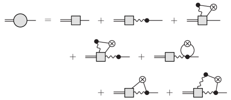
Figure 1: The diagrammatic representation of the two-point propagator with partially resummed vertex up to one-loop contributions.

Diagrammatic rules in iPT mat11 with the Lagrangian picture, which are explained in App. A, are applied in the correspondence. The normalized two-point propagator of mass density field, $\hat{\varGamma}^{(1)}_{\rm m}$, is obtained by putting $c^{(n)}_{X}=0$ in Eq. (8).

The perturbative expansion of the displacement field in Fourier space, $\tilde{\bm{\varPsi}}(\bm{k})$ is given by

$$\tilde{\bm{\varPsi}}(\bm{k})=\sum_{n=1}^{\infty}\frac{i}{n!}\int_{\bm{k}_{1\cdots n}=\bm{k}}\bm{L}^{(n)}(\bm{k}_{1},\ldots,\bm{k}_{n})\delta_{\rm L}(\bm{k}_{1})\cdots\delta_{\rm L}(\bm{k}_{n}),$$ (9)

where we adopt a notation,

$$\int_{\bm{k}_{1\cdots n}=\bm{k}}\cdots=\int\frac{d^{3}k_{1}}{(2\pi)^{3}}\cdots\frac{d^{3}k_{n}}{(2\pi)^{3}}(2\pi)^{3}\delta_{\rm D}^{3}\left(\bm{k}-\bm{k}_{1\cdots n}\right)\cdots.$$ (10)

Such notation as Eq. (10) is commonly used throughout this paper.

In real space, the kernels of LPT in the standard theory of gravity (in the Newtonian limit) are given by cat95

$$\bm{L}^{(1)}(\bm{k})=\frac{\bm{k}}{k^{2}},$$ (11)

$$\bm{L}^{(2)}(\bm{k}_{1},\bm{k}_{2})=\frac{3}{7}\frac{\bm{k}_{12}}{{k_{12}}^{2}}\left[1-\left(\frac{\bm{k}_{1}\cdot\bm{k}_{2}}{k_{1}k_{2}}\right)^{2}\right],$$ (12)

$$\bm{L}^{(3)}(\bm{k}_{1},\bm{k}_{2},\bm{k}_{3})=\frac{1}{3}\left[\bm{L}^{(3{\rm a})}(\bm{k}_{1},\bm{k}_{2},\bm{k}_{3})+{\rm perm.}\right];$$ (13)

$$\bm{L}^{(3{\rm a})}(\bm{k}_{1},\bm{k}_{2},\bm{k}_{3})$$

$$\quad=\frac{\bm{k}_{123}}{{k_{123}}^{2}}\left\{\frac{5}{7}\left[1-\left(\frac{\bm{k}_{1}\cdot\bm{k}_{2}}{k_{1}k_{2}}\right)^{2}\right]\left[1-\left(\frac{\bm{k}_{12}\cdot\bm{k}_{3}}{{k}_{12}k_{3}}\right)^{2}\right]\right.$$

$$\qquad\quad\left.-\frac{1}{3}\left[1-3\left(\frac{\bm{k}_{1}\cdot\bm{k}_{2}}{k_{1}k_{2}}\right)^{2}+\,2\frac{(\bm{k}_{1}\cdot\bm{k}_{2})(\bm{k}_{2}\cdot\bm{k}_{3})(\bm{k}_{3}\cdot\bm{k}_{1})}{{k_{1}}^{2}{k_{2}}^{2}{k_{3}}^{2}}\right]\right\}$$

$$\qquad+\frac{\bm{k}_{123}}{{k_{123}}^{2}}\times\bm{T}(\bm{k}_{1},\bm{k}_{2},\bm{k}_{3}),$$ (14)

where a vector function $\bm{T}$ represents a transverse part whose explicit expression will not be used in this paper. Complete expressions of the displacement kernels of LPT up to 4th order, including transverse parts are given in, e.g., Ref. RB12 ; tat13 . Eqs. (7) and (8) remain valid even when the non-standard theory of gravity is assumed as long as the appropriate form of kernels $\bm{L}_{n}$ in such a theory is used.

One of the benefits in the Lagrangian picture is that redshift-space distortions are relatively easy to be incorporated in the theory. A displacement kernel in redshift space $\bm{L}^{{\rm s}(n)}$ is simply related to the kernel in real space at the same order by a linear mapping mat08a ,

$$\bm{L}^{(n)}\rightarrow\bm{L}^{{\rm s}(n)}=\bm{L}^{(n)}+nf\left(\hat{\bm{z}}\cdot\bm{L}^{(n)}\right)\hat{\bm{z}},$$ (15)

where $f=d\ln D/d\ln a=\dot{D}/HD$ is the linear growth rate, $D(t)$ is the linear growth factor, $a(t)$ is the scale factor, and $H(t)=\dot{a}/a$ is the time-dependent Hubble parameter. The distant-observer approximation is assumed in redshift space, and the unit vector $\hat{\bm{z}}$ denotes the line-of-sight direction. Strictly speaking, the mapping of Eq. (15) is exact only in the Einstein-de Sitter universe. However, this mapping is a good approximation in general cosmology. The expressions of Eqs. (7) and (8) apply as well in redshift space when the displacement kernels in redshift space $\bm{L}^{{\rm s}(n)}$ are used instead of the real-space counterparts $\bm{L}^{(n)}$.

The three-point propagator at the tree-level approximation in iPT is given by

$$\hat{\varGamma}^{(2)}_{X}(\bm{k}_{1},\bm{k}_{2})=c^{(2)}_{X}(\bm{k}_{1},\bm{k}_{2})+c^{(1)}_{X}(\bm{k}_{1})\left[\bm{k}\cdot\bm{L}^{(1)}(\bm{k}_{2})\right]\\ +c^{(1)}_{X}(\bm{k}_{2})\left[\bm{k}\cdot\bm{L}^{(1)}(\bm{k}_{1})\right]+\left[\bm{k}\cdot\bm{L}^{(1)}(\bm{k}_{1})\right]\left[\bm{k}\cdot\bm{L}^{(1)}(\bm{k}_{2})\right]\\ +\bm{k}\cdot\bm{L}^{(2)}(\bm{k}_{1},\bm{k}_{2}),$$ (16)

where each term respectively corresponds to each diagram of Fig. 2 in the same order.

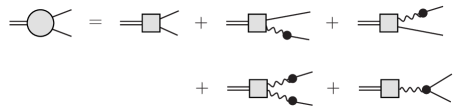
Figure 2: The diagrammatic representation of the three-point propagator with partially resummed vertex at the tree-level contribution.

When the mapping of Eq. (15) is applied to every displacement kernels in Eq. (16), the expression of three-point propagator in redshift space is obtained. The three-point propagator of mass, $\varGamma^{(2)}_{\rm m}$, is given by just substituting $c^{(n)}_{X}=0$ in Eq. (16).

In terms of the multi-point propagators, the power spectrum of biased objects, up to the one-loop approximation, is given by

$$P_{X}(\bm{k})=\varPi^{2}(k)\Biggl{\{}\left[\hat{\varGamma}^{(1)}_{X}(\bm{k})\right]^{2}P_{\rm L}(k)\\ +\frac{1}{2}\int_{\bm{k}_{12}=\bm{k}}\left[\hat{\varGamma}^{(2)}_{X}(\bm{k}_{1},\bm{k}_{2})\right]^{2}P_{\rm L}(k_{1})P_{\rm L}(k_{2})\\ +\hat{\varGamma}^{(1)}_{X}(\bm{k})\int_{\bm{k}_{12}=\bm{k}}\hat{\varGamma}^{(2)}_{X}(\bm{k}_{1},\bm{k}_{2})B_{\rm L}(k,k_{1},k_{2})\Biggr{\}},$$ (17)

where $P_{\rm L}(k)$ and $B_{\rm L}(k,k_{1},k_{2})$ are the linear power spectrum and the linear bispectrum, respectively. The diagrammatic representations of Eq. (17) are shown in Fig. 3.

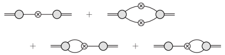
Figure 3: The diagrammatic representation of the power spectrum up to one-loop approximation.

Crossed circles correspond to the linear power spectrum or the linear bispectrum, depending on number of lines attached to them. The first two terms in Eq. (17) corresponds to the first two diagrams in Fig. 3. The last two diagrams in Fig. 3 are contributions from the primordial non-Gaussianity. The two diagrams give the same contribution because of the parity symmetry, and the sum of the two diagrams corresponds to the last term in Eq. (17).

The matter power spectrum $P_{\rm m}(\bm{k})$ is simply given by replacing $\varGamma^{(n)}_{X}$ by $\varGamma^{(n)}_{\rm m}$ in Eq. (17), or equivalently, setting $c^{(n)}_{X}=0$ for every $n\geq 1$. The cross power spectrum between two types of objects, $X$ and $Y$, is similarly obtained as

$$P_{XY}(\bm{k})=\varPi^{2}(k)\Biggl{\{}\hat{\varGamma}^{(1)}_{X}(\bm{k})\hat{\varGamma}^{(1)}_{Y}(\bm{k})P_{\rm L}(k)\\ +\frac{1}{2}\int_{\bm{k}_{12}=\bm{k}}\hat{\varGamma}^{(2)}_{X}(\bm{k}_{1},\bm{k}_{2})\hat{\varGamma}^{(2)}_{Y}(\bm{k}_{1},\bm{k}_{2})P_{\rm L}(k_{1})P_{\rm L}(k_{2})\\ +\frac{1}{2}\hat{\varGamma}^{(1)}_{X}(\bm{k})\int_{\bm{k}_{12}=\bm{k}}\hat{\varGamma}^{(2)}_{Y}(\bm{k}_{1},\bm{k}_{2})B_{\rm L}(k,k_{1},k_{2})\\ +\frac{1}{2}\hat{\varGamma}^{(1)}_{Y}(\bm{k})\int_{\bm{k}_{12}=\bm{k}}\hat{\varGamma}^{(2)}_{X}(\bm{k}_{1},\bm{k}_{2})B_{\rm L}(k,k_{1},k_{2})\Biggr{\}}.$$ (18)

The diagrams for the above equations are similar to the ones in Fig. 3, where the left and right multi-point propagators correspond to those of $X$ and $Y$, respectively. When $X=Y$, Eq. (18) apparently reduces to Eq. (17).

The predictions of biased power spectra in the one-loop approximation of iPT are given by Eq. (17) for the auto power spectrum, and by Eq. (18) for the cross power spectrum. Once a model of the renormalized bias functions $c^{(n)}_{X}$ is given, it is straightforward to numerically evaluate those equations. The above results are general and do not depend on bias models. Any bias model can be incorporated in the expression of iPT through the renormalized bias functions. In the next subsection, we explain a simple model of the renormalized bias function based on the halo approach.

II.2 Renormalized bias functions in a simple model of halo approach

The renormalized bias functions $c^{(n)}_{X}$ are not specified in the general framework of iPT. Precise modeling of bias is a nontrivial problem, depending on what kind of biased tracers are considered. In this subsection, we consider a simple model of halo bias as an example. The expressions of renormalized bias functions in a simple model of the halo approach are recently derived in Ref. mat12 . We summarize the consequences of this model below. It should be emphasized that the general framework of iPT does not depend on this specific model of bias.

Without resorting to approximations such as the peak-background split, the halo bias is shown to be nonlocal even in Lagrangian space. As a result, the renormalized bias functions have nontrivial scale dependencies. For the halos of mass $M$, the renormalized bias functions are given by mat12

$$c^{(n)}_{M}(\bm{k}_{1},\ldots,\bm{k}_{n})=b^{\rm L}_{n}(M)W(k_{1}R)\cdots W(k_{n}R)\\ +\frac{A_{n-1}(M)}{{\delta_{\rm c}}^{n}}\frac{d}{d\ln\sigma_{M}}\left[W(k_{1}R)\cdots W(k_{n}R)\right],$$ (19)

where $\delta_{\rm c}=3(3\pi/2)^{2/3}/5\simeq 1.686$ is the critical overdensity for spherical collapse and $W(kR)$ is a window function. In a usual halo approach, the window function is chosen to be a top-hat type in configuration space, which corresponds to

$$W(x)=\frac{3\sin x-3x\cos x}{x^{3}},$$ (20)

in Fourier space. In this case, the Lagrangian radius $R$ is naturally related to the mass $M$ of halo by

$$M=\frac{4}{3}\pi\bar{\rho}_{0}R^{3},$$ (21)

where $\bar{\rho}_{0}$ is the mean density of mass at the present time, or

$$R=\left[\frac{M}{1.163\times 10^{12}h^{-1}M_{\odot}\varOmega_{\rm m0}}\right]^{1/3}\,h^{-1}\rm{Mpc},$$ (22)

where $M_{\odot}=1.989\times 10^{30}\,{\rm kg}$ is the solar mass, $\varOmega_{\rm m0}$ is the density parameter of mass at the present time, and $h=H_{0}/(100\,\rm{km\,s^{-1}\,Mpc^{-1}})$ is the normalized Hubble constant.

Empirically, one can also use other types of window function. Direct evaluations of the renormalized bias functions suggest that Gaussian window function $W(x)=e^{-k^{2}R^{2}/2}$ gives better fit NMT14 . In the latter case, the relation between the smoothing radius $R$ and mass $M$ is not trivial and should also be empirically modified from the relation of Eq. (22). However, the shapes of one-loop power spectrum on large scales are not sensitive to the choice of window function.

The variance of density fluctuations on the mass scale $M$ is defined by

$${\sigma_{M}}^{2}=\int\frac{d^{3}k}{(2\pi)^{3}}W^{2}(kR)P_{\rm L}(k).$$ (23)

The radius $R$ is considered as a function of $\sigma_{M}$ through Eq. (19). The functions $A_{n}(M)$ are defined by

$$A_{n}(M)\equiv\sum_{j=0}^{n}\frac{n!}{j!}{\delta_{\rm c}}^{j}\,b^{\rm L}_{j}(M),$$ (24)

where $b^{\rm L}_{n}$ is the scale-independent Lagrangian bias parameter of $n$th-order. For example, first three functions are given by

$$A_{0}=1,\quad A_{1}=1+\delta_{\rm c}b^{\rm L}_{1},\quad A_{2}=2+2\delta_{\rm c}b^{\rm L}_{1}+{\delta_{\rm c}}^{2}b^{\rm L}_{2}.$$ (25)

When the halo mass function $n(M)$ takes a universal form

$$n(M)dM=\frac{\bar{\rho}_{0}}{M}f_{\rm MF}(\nu)\frac{d\nu}{\nu},$$ (26)

where $\nu=\delta_{\rm c}/\sigma_{M}$, the Lagrangian bias parameters are given by

$$b^{\rm L}_{n}(M)=\left(\frac{-1}{\sigma_{M}}\right)^{n}\frac{f_{\rm MF}^{(n)}(\nu)}{f_{\rm MF}(\nu)},$$ (27)

where $f_{\rm MF}^{(n)}=d^{n}f_{\rm MF}/d\nu^{n}$.

Once the model of the mass function $f_{\rm MF}(\nu)$ is given, the scale-independent bias parameters $b^{\rm L}_{n}(M)$ and the functions $A_{n}(M)$ are uniquely given by Eqs. (27) and (24). In Table 1, those functions are summarized for popular models of mass function, i.e., the Press-Schechter (PS) mass function PS74 , the Sheth-Tormen (ST) mass function ST99 , Warren et al. (W+) mass function War06 .

	PS	ST	W+, MICE ($\sigma=\delta_{\rm c}/\nu$)
$f_{\rm MF}(\nu)$	$\displaystyle\sqrt{\frac{2}{\pi}}\,\nu e^{-\nu^{2}/2}$	$\displaystyle A(p)\sqrt{\frac{2}{\pi}}\left[1+\frac{1}{(q\nu^{2})^{p}}\right]\sqrt{q}\,\nu e^{-q\nu^{2}/2}$	$\displaystyle A\left(\sigma^{-a}+b\right)e^{-c/\sigma^{2}}$
$b^{\rm L}_{1}(M)$	$\displaystyle\frac{\nu^{2}-1}{\delta_{\rm c}}$	$\displaystyle\frac{1}{\delta_{\rm c}}\left[q\nu^{2}-1+\frac{2p}{1+(q\nu^{2})^{p}}\right]$	$\displaystyle\frac{1}{\delta_{\rm c}}\left(\frac{2c}{\sigma^{2}}-\frac{a}{1+b\sigma^{a}}\right)$
$b^{\rm L}_{2}(M)$	$\displaystyle\frac{\nu^{4}-3\nu^{2}}{{\delta_{\rm c}}^{2}}$	$\displaystyle\frac{1}{{\delta_{\rm c}}^{2}}\left[q^{2}\nu^{4}-3q\nu^{2}+\frac{2p(2q\nu^{2}+2p-1)}{1+(q\nu^{2})^{p}}\right]$	$\displaystyle\frac{1}{{\delta_{\rm c}}^{2}}\left[\frac{4c^{2}}{\sigma^{4}}-\frac{2c}{\sigma^{2}}-\frac{a\left(4c/\sigma^{2}-a+1\right)}{1+b\sigma^{a}}\right]$
$A_{1}(M)$	$\nu^{2}$	$\displaystyle q\nu^{2}+\frac{2p}{1+(q\nu^{2})^{p}}$	$\displaystyle\frac{2c}{\sigma^{2}}+1-\frac{a}{1+b\sigma^{a}}$
$A_{2}(M)$	$\nu^{2}(\nu^{2}-1)$	$\displaystyle q\nu^{2}(q\nu^{2}-1)+\frac{2p(2q\nu^{2}+2p+1)}{1+(q\nu^{2})^{p}}$	$\displaystyle\frac{4c^{2}}{\sigma^{4}}+\frac{2c}{\sigma^{2}}+2-\frac{a\left(4c/\sigma^{2}-a+3\right)}{1+b\sigma^{a}}$
Parameters	-	$\begin{array}[]{c}A(p)=[1+\pi^{-1/2}2^{-p}\varGamma(1/2-p)]^{-1}\\ p=0.3\\ q=0.707\end{array}$	$\begin{array}[]{l}\mbox{W+}:\\ A=0.7234\\ a=1.625\\ b=0.2538\\ c=1.1982\end{array}$ $\begin{array}[]{l}\mbox{MICE}:\\ A(z)=0.58(1+z)^{-0.13}\\ a(z)=1.37(1+z)^{-0.15}\\ b(z)=0.3(1+z)^{-0.084}\\ c(z)=1.036(1+z)^{-0.024}\end{array}$

Table 1: Functions $b^{\rm L}_{n}(M)$, $A_{n}(M)$ derived from several models of mass function.

In the simplest PS mass function, it is interesting to note that general expressions of the parameters for all orders can be derived mat12 : $b^{\rm L}_{n}=\nu^{n-1}H_{n+1}(\nu)/{\delta_{\rm c}}^{n}$, $A_{n}=\nu^{n}H_{n}(\nu)$, where $H_{n}(\nu)$ are the Hermite polynomials. The ST mass function gives a better fit to numerical simulations of halos in cold-dark-matter type cosmologies with Gaussian initial conditions. The values of parameters in Table 1 are $p=0.3$, $q=0.707$, and $A(p)=[1+\pi^{-1/2}2^{-p}\varGamma(1/2-p)]^{-1}$ is the normalization factor. When we put $p=0$, $q=1$, the ST mass function reduces to the PS mass function. The W+ mass function is represented by a parameter $\sigma=\delta_{\rm c}/\nu$, which is also a function of $M$, and parameters are $A=0.7234$, $a=1.625$, $b=0.2538$, $c=1.1982$. The same functional form is applied to the Marenostrum Institut de Ciéncies de l’Espai (MICE) simulations in Ref. Cro10 , allowing the parameters redshift-dependent. Their values are given by $A(z)=0.58(1+z)^{-0.13}$, $a(z)=1.37(1+z)^{-0.15}$, $b(z)=0.3(1+z)^{-0.084}$, $c(z)=1.036(1+z)^{-0.024}$. When the redshift-dependent parameters are adopted, the W+ mass function is sometimes referred to as the “MICE mass function”. In the latter case, the multiplicity function $f_{\rm MF}(\nu)$ explicitly depends on the redshift, and the mass function is no longer ’universal’.

The nonlocal nature of the halo bias in Lagrangian space is encoded in the second term in the RHS of Eq. (19), since the simple dependence on the window function of the first term appears even in the local bias models through the smoothed mass density field. In the large-scale limit, $k_{1},k_{2},\ldots,k_{n}\rightarrow 0$, the second term in the RHS of Eq. (19) disappears and the renormalized bias functions reduce to scale-independent bias parameters, $c^{(n)}_{M}\simeq b^{\rm L}_{n}(M)$. This property is consistent with the peak-background split. However, the loop corrections in the iPT involve integrations over the wavevectors of the renormalized bias functions, and there is no reason to neglect the second term which represents nonlocal nature of Lagrangian bias of halos.

The Eq. (19) is shown to be equivalent to the following expression mat12 ,

$$c^{(n)}_{M}(\bm{k}_{1},\ldots,\bm{k}_{n})=\frac{A_{n}(M)}{{\delta_{\rm c}}^{n}}W(k_{1}R)\cdots W(k_{n}R)\\ +\frac{A_{n-1}(M)\,{\sigma_{M}}^{n}}{{\delta_{\rm c}}^{n}}\frac{d}{d\ln\sigma_{M}}\left[\frac{W(k_{1}R)\cdots W(k_{n}R)}{{\sigma_{M}}^{n}}\right].$$ (28)

For the PS mass function, there is an interesting relation, $A_{n}=\nu^{2}{\delta_{\rm c}}^{n-1}b^{\rm L}_{n-1}$, and in this case, the renormalized bias function $c^{\rm L}_{n}$ is expressible by lower-order parameters $b^{\rm L}_{n-1}$ and $b^{\rm L}_{n-2}$, which is a reason why the scale-dependent bias in the presence of primordial non-Gaussianity is approximately proportional to the first-order bias parameter, $b^{\rm L}_{1}$ rather than the second-order one, $b^{\rm L}_{2}$ mat12 . However, this does not mean that $c^{(n)}_{M}$ is independent on $b^{\rm L}_{n}$, because $b^{\rm L}_{n}$ can be expressible by a linear combination of $b^{\rm L}_{n-1}$ and $b^{\rm L}_{n-2}$ in the PS mass function.

In the expressions of renormalized bias functions, Eqs. (19) and (28), all the halos are assumed to have the same mass, $M$. These expressions apply when the mass range of halos in a given sample is sufficiently narrow. When the mass range is finitely extended, the expressions should be replaced by mat12

$$c^{(n)}_{\phi}(\bm{k}_{1},\ldots,\bm{k}_{n})=\frac{\int dM\,\phi(M)\,n(M)\,c^{(n)}_{M}(\bm{k}_{1},\ldots,\bm{k}_{n})}{\int dM\,\phi(M)\,n(M)},$$ (29)

where $n(M)$ is the halo mass function of Eq. (26), $\phi(M)$ is a selection function of mass. For a simple example, when the mass of halos are selected by a finite range $[M_{1},M_{2}]$, we have

$$c^{(n)}_{[M_{1},M_{2}]}(\bm{k}_{1},\ldots,\bm{k}_{n})=\frac{\int_{M_{1}}^{M_{2}}dM\,n(M)\,c^{(n)}_{M}(\bm{k}_{1},\ldots,\bm{k}_{n})}{\int_{M_{1}}^{M_{2}}dM\,n(M)}.$$ (30)

III Explicit Formulas

The auto power spectrum $P_{X}(\bm{k})$ of Eq. (17) is a special case of the cross power spectrum $P_{XY}(\bm{k})$ of Eq. (18) as the former is given by setting $X=Y$ in the latter. It is general enough to give the formulas for the cross power spectrum below. In the following, we decompose Eq. (18) into the following form:

$$P_{XY}(\bm{k})=\varPi^{2}(\bm{k})\left[R_{XY}(\bm{k})+Q_{XY}(\bm{k})+S_{XY}(\bm{k})\right],$$ (31)

where $\varPi(\bm{k})$ is given by Eq. (7) and

$$R_{XY}(\bm{k}) =\hat{\varGamma}^{(1)}_{X}(\bm{k})\hat{\varGamma}^{(1)}_{Y}(\bm{k})P_{\rm L}(k),$$ (32)

$$Q_{XY}(\bm{k}) =\frac{1}{2}\int_{\bm{k}_{12}=\bm{k}}\hat{\varGamma}^{(2)}_{X}(\bm{k}_{1},\bm{k}_{2})\hat{\varGamma}^{(2)}_{Y}(\bm{k}_{1},\bm{k}_{2})P_{\rm L}(k_{1})P_{\rm L}(k_{2}),$$ (33)

$$S_{XY}(\bm{k}) =\frac{1}{2}\hat{\varGamma}^{(1)}_{X}(\bm{k})\int_{\bm{k}_{12}=\bm{k}}\hat{\varGamma}^{(2)}_{Y}(\bm{k}_{1},\bm{k}_{2})B_{\rm L}(k,k_{1},k_{2})$$

$$\qquad+(X\leftrightarrow Y).$$ (34)

Three-dimensional integrals appeared in the above components of Eqs. (32)–(34) can be reduced to lower-dimensional integrals both in real space and in redshift space. Such dimensional reductions of the integrals are useful for practical calculations. The purpose of this section is to give explicit formulas for the above components $\varPi$, $R_{XY}$, $Q_{XY}$, $S_{XY}$ in terms of two-dimensional integrals at most. The results of this section are applicable to any bias models, and do not depend on specific forms of renormalized bias functions, e.g., those explained in Sec. II.2.

III.1 The power spectra in real space

In real space, the power spectrum is independent on the direction of wavevector $\bm{k}$, and thus the components above $\varPi(k)$, $R_{XY}(k)$, $Q_{XY}(k)$, $S_{XY}(k)$ are also independent on the direction. In this case, dimensional reductions of the integrals in Eqs. (32)–(34) are not difficult, because of the rotational symmetry. The vertex resummation factor $\varPi(\bm{k})$ of Eq. (7) is given by

$$\varPi(k)=\exp\left[-\frac{k^{2}}{12\pi^{2}}\int dp\,P_{\rm L}(p)\right].$$ (35)

On small scales, this factor exponentially suppresses the power too much, and such a behavior is not physical. This property is a good indicator of which scales the perturbation theory should not be applied. However, the resummation of the vertex factor is not compulsory in the iPT. When the vertex factor is not resummed, one can expand the factor as

$$\varPi(k)=1-\frac{k^{2}}{12\pi^{2}}\int dp\,P_{\rm L}(p),$$ (36)

instead of Eq. (35) in the case of one-loop perturbation theory. In a quasi-linear regime, the resummed vertex factor of Eq. (35) gives better fit to $N$-body simulations in real space mat08a ; SM11 .

The expression of two-point propagator in Eq. (8) is straightforwardly obtained, substituting the Lagrangian kernels of Eqs. (11)–(14). Taking the $z$-axis of $\bm{p}$ as the direction of $\bm{k}$, integrations by the azimuthal angle are trivial. Transforming the rest of integration variables as $r=p/k$ and $x=\hat{\bm{p}}\cdot\hat{\bm{k}}$, we have two equivalent expressions,

$$\hat{\varGamma}^{(1)}_{X}(k) =1+c^{(1)}_{X}(k)+\frac{k^{3}}{4\pi^{2}}\int_{0}^{\infty}dr\int_{-1}^{1}dx\,\hat{\cal R}_{X}(k,r,x)P_{\rm L}(kr)$$ (37)

$$=1+c^{(1)}_{X}(k)+\frac{k^{3}}{4\pi^{2}}\int_{0}^{\infty}dr\,\tilde{\cal R}_{X}(k,r)P_{\rm L}(kr),$$ (38)

where

$$\hat{\cal R}_{X}(k,r,x)=\frac{5}{21}\frac{r^{2}(1-x^{2})^{2}}{1+r^{2}-2rx}\\ +\frac{3}{7}\frac{(1-rx)(1-x^{2})}{1+r^{2}-2rx}\left[rx+r^{2}c^{(1)}_{X}(kr)\right]\\ -rx\,c^{(2)}_{X}(k,kr;x),$$ (39)

and

$$\tilde{\cal R}_{X}(k,r)=\frac{6+5r^{2}+50r^{4}-21r^{6}}{252r^{2}}\\ +\frac{(1-r^{2})^{3}(2+7r^{2})}{168r^{3}}\ln\left|\frac{1-r}{1+r}\right|\\ +\left[\frac{3+8r^{2}-3r^{4}}{28}+\frac{3(1-r^{2})^{3}}{56r}\ln\left|\frac{1-r}{1+r}\right|\right]c^{(1)}_{X}(kr)\\ -r\int_{-1}^{1}dx\,x\,c^{(2)}_{X}(k,kr;x).$$ (40)

In the above expressions, rotationally invariant arguments for $c^{(2)}_{X}$ are used, i.e.,

$$c^{(2)}_{X}(\bm{k}_{1},\bm{k}_{2})=c^{(2)}_{X}(k_{1},k_{2};x),$$ (41)

where $x=\hat{\bm{k}}_{1}\cdot\hat{\bm{k}}_{2}$ is the direction cosine between $\bm{k}_{1}$ and $\bm{k}_{2}$. The second expression of Eq. (38) is obtained by analytically integrating the variable $x$ in the first expression of Eq. (37). Both expressions are suitable for numerical evaluations. With the expression of Eq. (37) or (38), we have

$$R_{XY}(k)=\hat{\varGamma}^{(1)}_{X}(k)\hat{\varGamma}^{(1)}_{Y}(k)P_{\rm L}(k).$$ (42)

Evaluating the convolution integrals in Eqs. (33) and (34) with the three-point propagator of Eq. (16) is also straightforward in real space. Substituting the Lagrangian kernels of Eqs. (11) and (12) into Eq. (16), and transforming the integration variables as $r=k_{1}/k$, $x=\hat{\bm{k}}\cdot\hat{\bm{k}_{1}}$, we have

$$Q_{XY}(k)=\frac{k^{3}}{8\pi^{2}}\int_{0}^{\infty}dr\int_{-1}^{1}dx\,r^{2}\hat{\varGamma}^{(2)}_{X}(k,r,x)\hat{\varGamma}^{(2)}_{Y}(k,r,x)\\ \times P_{\rm L}(kr)P_{\rm L}(ky)$$ (43)

and

$$S_{XY}(k)=\frac{k^{3}}{8\pi^{2}}\hat{\varGamma}^{(1)}_{X}(k)\int_{0}^{\infty}dr\int_{-1}^{1}dx\,r^{2}\hat{\varGamma}^{(2)}_{Y}(k,r,x)\\ \times B_{\rm L}(k,kr,ky)+(X\leftrightarrow Y),$$ (44)

where

$$y=\sqrt{1+r^{2}-2rx},$$ (45)

and

$$\hat{\varGamma}^{(2)}_{X}(k,r,x)=-\frac{4}{7}\,\frac{1-x^{2}}{y^{2}}+\frac{x}{r}\left[1+c^{(1)}_{X}(ky)\right]\\ +\frac{1-rx}{y^{2}}\left[1+c^{(1)}_{X}(kr)\right]+c^{(2)}_{X}(kr,ky;x),$$ (46)

The factor $\hat{\varGamma}^{(2)}_{Y}(k,r,x)$ is similarly given by substituting $X\rightarrow Y$ in Eq. (46). The function $\hat{\varGamma}^{(2)}_{X}(k,r,x)$ is just the normalized three-point propagator $\hat{\varGamma}^{(2)}_{X}(\bm{k}_{1},\bm{k}-\bm{k}_{1})$ as a function of transformed variables.

All the necessary components to calculate the power spectrum of Eq. (31) in real space,

$$P_{XY}(k)=\varPi^{2}(k)\left[R_{XY}(k)+Q_{XY}(k)+S_{XY}(k)\right],$$ (47)

are given above, i.e., Eqs. (35) [or (36)], (42), (43) and (44). Numerical integrations of Eqs. (38) [or (37)], (43) and (44) are not difficult, once the model of renormalized bias functions $c^{(n)}_{X}$ and primordial spectra $P_{\rm L}(k)$, $B_{\rm L}(k_{1},k_{2},k_{3})$ are given. The last factor $S_{XY}(k)$ is absent in the case of Gaussian initial conditions.

III.2 Kernel integrals

Evaluations of power spectra in redshift space are more tedious than those in real space. The reason is that the power spectra depend on the lines-of-sight direction in redshift space. One cannot arbitrary choose the direction of $z$-axis in the three-dimensional integrations of Eqs. (8) and (32)–(34), because the rotational symmetry is not met. Even in such cases, an axial symmetry around the lines of sight remains, and the three-dimensional integrations can be reduced to two- or one-dimensional integrations as shown below. All the necessary techniques for such reductions are the same with those presented in Refs. mat08a ; mat08b , making use of rotational covariance. We summarize useful formulas for the reduction in this subsection. We assume the standard theory of gravity in the formula below, although the same technique may be applicable to other theories such as the modified gravity, etc.

The first set of formulas is related to the two-point propagator $\varGamma^{(1)}_{X}$ of Eq. (8). The results are summarized in Table 2. The integrals of a form,

$$\vphantom{\frac{\int}{\int}}\int\frac{d^{3}p}{(2\pi)^{3}}{\cal F}(\bm{k},\bm{p})P_{\rm L}(p),$$ (48)

where ${\cal F}(\bm{k},\bm{p})$ consists of LPT kernels $\bm{L}^{(n)}$ and renormalized bias functions $c^{(n)}_{X}$, are reduced to one-dimensional integrals, $R^{X}_{n}(k)$. The explicit formulas are given in Table 2.

$\displaystyle{\cal F}(\bm{k},\bm{p})$	$\displaystyle\vphantom{\frac{\int}{\int}}\int\frac{d^{3}p}{(2\pi)^{3}}{\cal F}(\bm{k},\bm{p})P_{\rm L}(p)$	Diagram
$\displaystyle\bm{L}^{(3)}(\bm{k},\bm{p},-\bm{p})$	$\displaystyle\vphantom{\frac{\int}{\int}}\frac{10}{21}\frac{\bm{k}}{k^{2}}R_{1}(k)$
$\displaystyle L^{(1)}_{i}(-\bm{p})L^{(2)}_{j}(\bm{k},\bm{p})$	$\displaystyle\vphantom{\frac{\int}{\int}}\frac{3}{14}\frac{k_{i}k_{j}-k^{2}\delta_{ij}}{k^{4}}R_{1}(k)+\frac{3}{7}\frac{k_{i}k_{j}}{k^{4}}R_{2}(k)$
$\displaystyle\bm{L}^{(2)}(\bm{k},\bm{p})c^{(1)}_{X}(p)$	$\displaystyle\vphantom{\frac{\int}{\int}}\frac{3}{7}\frac{\bm{k}}{k^{2}}R_{3}^{X}(k)$
$\displaystyle\bm{L}^{(1)}(-\bm{p})c^{(2)}_{X}(\bm{k},\bm{p})$	$\displaystyle\vphantom{\frac{\int}{\int}}-\frac{\bm{k}}{k^{2}}R_{4}^{X}(k)$

Table 2: Integral formulas for one-loop corrections, which are related to the two-point propagator. We denote $R_{1}(k)=R_{1}^{X}(k)$ and $R_{2}(k)=R_{2}^{X}(k)$, as these functions are independent on the bias.

In this Table, we denote $R_{1}(k)=R_{1}^{X}(k)$ and $R_{2}(k)=R_{2}^{X}(k)$, as these functions are independent on the bias. The functions $R^{X}_{n}(k)$ are defined by three equivalent sets of equations,

$$R^{X}_{n}(k) =\int\frac{d^{3}p}{(2\pi)^{3}}{\cal R}^{X}_{n}(\bm{k},\bm{p})P_{\rm L}(p)$$

$$=\frac{k^{3}}{4\pi^{2}}\int_{0}^{\infty}dr\int_{-1}^{1}dx\,\hat{\cal R}^{X}_{n}(r,x)P_{\rm L}(kr)$$

$$=\frac{k^{3}}{4\pi^{2}}\int_{0}^{\infty}dr\,\tilde{\cal R}^{X}_{n}(r)P_{\rm L}(kr),$$ (49)

where integrands ${\cal R}^{X}_{n}(\bm{k},\bm{p})$, $\hat{\cal R}^{X}_{n}(r,x)$, and $\tilde{\cal R}^{X}_{n}(r)$ are given in Table 3.

$n$	${\cal R}^{X}_{n}(\bm{k},\bm{p})$	$\hat{\cal R}^{X}_{n}(r,x)$	$\tilde{\cal R}^{X}_{n}(r)$
$1$	$\displaystyle\frac{k^{2}}{|\bm{k}-\bm{p}|^{2}}\left[1-\left(\frac{\bm{k}\cdot\bm{p}}{kp}\right)^{2}\right]^{2}$	$\displaystyle\frac{r^{2}(1-x^{2})^{2}}{1+r^{2}-2rx}$	$\displaystyle-\frac{(1+r^{2})(3-14r^{2}+3r^{4})}{24r^{2}}-\frac{(1-r^{2})^{4}}{16r^{3}}\ln\left|\frac{1-r}{1+r}\right|$
$2$	$\displaystyle\frac{\left(\bm{k}\cdot\bm{p}\right)\left[\bm{k}\cdot(\bm{k}-\bm{p})\right]}{p^{2}|\bm{k}-\bm{p}|^{2}}\left[1-\left(\frac{\bm{k}\cdot\bm{p}}{kp}\right)^{2}\right]$	$\displaystyle\frac{rx(1-rx)(1-x^{2})}{1+r^{2}-2rx}$	$\displaystyle\frac{(1-r^{2})(3-2r^{2}+3r^{4})}{24r^{2}}+\frac{(1-r^{2})^{3}(1+r^{2})}{16r^{3}}\ln\left|\frac{1-r}{1+r}\right|$
$3$	$\displaystyle\frac{\bm{k}\cdot(\bm{k}-\bm{p})}{|\bm{k}-\bm{p}|^{2}}\left[1-\left(\frac{\bm{k}\cdot\bm{p}}{kp}\right)^{2}\right]c^{(1)}_{X}(p)$	$\displaystyle\frac{r^{2}(1-rx)(1-x^{2})}{1+r^{2}-2rx}c^{(1)}_{X}(kr)$	$\displaystyle\left[\frac{3+8r^{2}-3r^{4}}{12}+\frac{(1-r^{2})^{3}}{8r}\ln\left|\frac{1-r}{1+r}\right|\right]c^{(1)}_{X}(kr)$
$4$	$\displaystyle\frac{\bm{k}\cdot\bm{p}}{p^{2}}c^{(2)}_{X}(\bm{k},\bm{p})$	$\displaystyle rx\,c^{(2)}_{X}(k,kr;x)$	$\displaystyle r\int_{-1}^{1}dx\,x\,c^{(2)}_{X}(k,kr;x)$

Table 3: Integrands for functions $R^{X}_{n}(k)$ of Eq. (49).

The last expression of Eq. (49) is the formula which is practically useful for numerical evaluations. The other expressions are shown to indicate origins of the integrals.

If the second-order bias function $c^{(2)}_{X}(\bm{k}_{1},\bm{k}_{2})$ only depends on magnitudes of wavevectors $k_{1}$ and $k_{2}$, and not on the relative angle $\mu_{12}=\hat{\bm{k}_{1}}\cdot\hat{\bm{k}_{2}}$, the fourth function generically vanishes: $R^{X}_{4}(k)=0$. If the first-order bias function $c^{(1)}_{X}$ is scale-independent, it is explicitly shown from the last expressions that $R^{X}_{3}(k)=[R_{1}(k)+R_{2}(k)]c^{(1)}_{X}$. Specifically, the functions $R^{X}_{3}(k)$ and $R^{X}_{4}(k)$ are redundant in the Lagrangian local bias models, in which renormalized bias functions $c^{(n)}_{X}$ are scale-independent. This is the reason only two functions $R_{1}(k)$ and $R_{2}(k)$ are needed in Ref. mat08b . In general situations with Lagrangian nonlocal bias models, all four functions are needed. In a simple model of halo bias in this paper, the second-order bias function $c^{(2)}_{X}$ does not depend on the angle $\mu_{12}$ and $R_{4}(k)=0$ in this case.

The second set of formulas is related to the convolution integrals of the three-point propagators $\varGamma^{(2)}_{X}$ in calculating the one-loop power spectrum. The integrals of the form,

$$\int_{\bm{k}_{12}=\bm{k}}{\cal F}(\bm{k}_{1},\bm{k}_{2})P_{\rm L}(k_{1})P_{\rm L}(k_{2}),$$ (50)

where ${\cal F}$ consists of LPT kernels $\bm{L}_{n}$ and renormalized bias functions $c^{(n)}_{X}$ and $c^{(n)}_{Y}$, are reduced to two-dimensional integrals, $Q^{XY}_{n}(k)$. The explicit formulas are given Table 4.

$\displaystyle{\cal F}(\bm{k}_{1},\bm{k}_{2})$	$\displaystyle\vphantom{\frac{\int}{\int}}\int_{\bm{k}_{12}=\bm{k}}{\cal F}(\bm{k}_{1},\bm{k}_{2})P_{\rm L}(k_{1})P_{\rm L}(k_{2})$	Diagram
$\displaystyle L^{(2)}_{i}(\bm{k}_{1},\bm{k}_{2})L^{(2)}_{j}(\bm{k}_{1},\bm{k}_{2})$	$\displaystyle\vphantom{\frac{\int}{\int}}\frac{9}{49}\frac{k_{i}k_{j}}{k^{4}}Q_{1}(k)$
$\displaystyle L^{(1)}_{i}(\bm{k}_{1})L^{(1)}_{j}(\bm{k}_{2})L^{(2)}_{k}(\bm{k}_{1},\bm{k}_{2})$	$\displaystyle\vphantom{\frac{\int}{\int}}\frac{3}{14}\frac{(k_{i}k_{j}-k^{2}\delta_{ij})k_{k}}{k^{6}}Q_{1}(k)+\frac{3}{7}\frac{k_{i}k_{j}k_{k}}{k^{6}}Q_{2}(k)$
$\displaystyle L^{(1)}_{(i}(\bm{k}_{1})L^{(1)}_{j}(\bm{k}_{1})L^{(1)}_{k}(\bm{k}_{2})L^{(1)}_{l)}(\bm{k}_{2})$	$\displaystyle\begin{array}[]{l}\displaystyle\vphantom{\frac{\int}{\int}}\frac{3}{8}\,\frac{k_{i}k_{j}k_{k}k_{l}-2k^{2}\delta_{(ij}k_{k}k_{l)}+k^{4}\delta_{(ij}\delta_{kl)}}{k^{8}}Q_{1}(k)\\ \displaystyle\vphantom{\frac{\int}{\int}}\qquad-\frac{1}{2}\,\frac{k_{i}k_{j}k_{k}k_{l}-k^{2}\delta_{(ij}k_{k}k_{l)}}{k^{8}}Q_{3}(k)+\frac{k_{i}k_{j}k_{k}k_{l}}{k^{8}}Q_{4}(k)\end{array}$
$\displaystyle\vphantom{\frac{\int}{\int}}L^{(1)}_{i}(\bm{k}_{1})L^{(2)}_{j}(\bm{k}_{1},\bm{k}_{2})c^{(1)}_{X}(k_{2})$	$\displaystyle\frac{3}{7}\,\frac{k_{i}k_{j}}{k^{4}}Q^{X}_{5}(k)$
$\displaystyle\vphantom{\frac{\int}{\int}}L^{(1)}_{(i}(\bm{k}_{1})L^{(1)}_{j}(\bm{k}_{1})L^{(1)}_{k)}(\bm{k}_{2})c^{(1)}_{X}(k_{2})$	$\displaystyle-\frac{1}{2}\,\frac{k_{i}k_{j}k_{l}-k^{2}\delta_{(ij}k_{k)}}{k^{6}}Q^{X}_{6}(k)+\frac{k_{i}k_{j}k_{k}}{k^{6}}Q^{X}_{7}(k)$
$\displaystyle\vphantom{\frac{\int}{\int}}\bm{L}^{(2)}(\bm{k}_{1},\bm{k}_{2})c^{(2)}_{X}(\bm{k}_{1},\bm{k}_{2})$	$\displaystyle\frac{3}{7}\frac{\bm{k}}{k^{2}}Q^{X}_{8}(k)$
$\displaystyle\vphantom{\frac{\int}{\int}}L^{(1)}_{i}(\bm{k}_{1})L^{(1)}_{j}(\bm{k}_{2})c^{(2)}_{X}(\bm{k}_{1},\bm{k}_{2})$	$\displaystyle\frac{1}{2}\,\frac{k_{i}k_{j}-k^{2}\delta_{ij}}{k^{4}}Q^{X}_{8}(k)+\frac{k_{i}k_{j}}{k^{4}}Q^{X}_{9}(k)$
$\displaystyle\vphantom{\frac{\int}{\int}}L^{(1)}_{i}(\bm{k}_{1})L^{(1)}_{j}(\bm{k}_{2})c^{(1)}_{X}(k_{1})c^{(1)}_{Y}(k_{2})$	$\displaystyle\frac{1}{2}\,\frac{k_{i}k_{j}-k^{2}\delta_{ij}}{k^{4}}Q^{XY}_{10}(k)+\frac{k_{i}k_{j}}{k^{4}}Q^{XY}_{11}(k)$
$\displaystyle\vphantom{\frac{\int}{\int}}L^{(1)}_{i}(\bm{k}_{1})L^{(1)}_{j}(\bm{k}_{1})c^{(1)}_{X}(k_{2})c^{(1)}_{Y}(k_{2})$	$\displaystyle-\frac{1}{2}\,\frac{k_{i}k_{j}-k^{2}\delta_{ij}}{k^{4}}Q^{XY}_{12}(k)+\frac{k_{i}k_{j}}{k^{4}}Q^{XY}_{13}(k)$
$\displaystyle\vphantom{\frac{\int}{\int}}\bm{L}^{(1)}(\bm{k}_{1})c^{(1)}_{X}(k_{2})c^{(2)}_{Y}(\bm{k}_{1},\bm{k}_{2})$	$\displaystyle\frac{\bm{k}}{k^{2}}Q^{XY}_{14}(k)$
$\displaystyle\vphantom{\frac{\int}{\int}}c^{(2)}_{X}(\bm{k}_{1},\bm{k}_{2})c^{(2)}_{Y}(\bm{k}_{1},\bm{k}_{2})$	$\displaystyle Q^{XY}_{15}(k)$

Table 4: Integral formulas for one-loop corrections, which are related to convolving three-point propagators. In the third and fifth formulas, the spatial indices are completely symmetrized. We denote $Q_{n}(k)=Q^{XY}_{n}(k)$ for $n=1,2,3,4$, as these functions are independent on the bias, and $Q^{X}_{n}(k)=Q^{XY}_{n}(k)$ for $n=5,6,7,8,9$, as these functions are only dependent on the bias of objects $X$.

For the third and fifth formulas in this Table, the indices of the LPT kernels are symmetrized, since only symmetric combinations are used in this paper. In this Table, we denote $Q_{n}(k)=Q^{XY}_{n}(k)$ for $n=1,2,3,4$, as these functions are independent on the bias, and $Q^{X}_{n}(k)=Q^{XY}_{n}(k)$ for $n=5,6,7,8,9$, as these functions are only dependent on the bias of objects $X$.

The functions $Q^{XY}_{n}(k)$ are defined by two equivalent sets of equations,

$$Q^{XY}_{n}(k) =\int_{\bm{k}_{12}=\bm{k}}{\cal Q}^{XY}_{n}(\bm{k}_{1},\bm{k}_{2})P_{\rm L}(k_{1})P_{\rm L}(k_{2})$$

$$=\frac{k^{3}}{4\pi^{2}}\int_{0}^{\infty}dr\int_{-1}^{1}dx\,\tilde{\cal Q}^{XY}_{n}(r,x)P_{\rm L}(kr)$$

$$\hskip 84.0pt\times P_{\rm L}\left(k\sqrt{1+r^{2}-2rx}\right),$$ (51)

where integrands ${\cal Q}^{XY}_{n}(\bm{k}_{1},\bm{k}_{2})$, $\tilde{\cal Q}^{XY}_{n}(r,x)$ are given in Table 5.

$n$	$\begin{array}[]{c}{\cal Q}^{XY}_{n}(\bm{k}_{1},\bm{k}_{2})\\ \left[\bm{k}=\bm{k}_{1}+\bm{k}_{2}\right]\end{array}$	$\begin{array}[]{c}\tilde{\cal Q}^{XY}_{n}(r,x)\\ \left[\begin{array}[]{c}y=(1+r^{2}-2rx)^{1/2},\\ \mu=(x-r)/y\end{array}\right]\end{array}$
$1$	$\displaystyle\vphantom{\frac{\int}{\int}}\left[1-\left(\frac{\bm{k}_{1}\cdot\bm{k}_{2}}{k_{1}k_{2}}\right)^{2}\right]^{2}$	$\displaystyle\frac{r^{2}(1-x^{2})^{2}}{y^{4}}$
$2$	$\displaystyle\vphantom{\frac{\int}{\int}}\frac{(\bm{k}\cdot\bm{k}_{1})(\bm{k}\cdot\bm{k}_{2})}{{k_{1}}^{2}{k_{2}}^{2}}\left[1-\left(\frac{\bm{k}_{1}\cdot\bm{k}_{2}}{k_{1}k_{2}}\right)^{2}\right]$	$\displaystyle\frac{rx(1-rx)(1-x^{2})}{y^{4}}$
$3$	$\displaystyle\vphantom{\frac{\int}{\int}}\frac{k^{4}-6(\bm{k}\cdot\bm{k}_{1})(\bm{k}\cdot\bm{k}_{2})}{{k_{1}}^{2}{k_{2}}^{2}}\left[1-\left(\frac{\bm{k}_{1}\cdot\bm{k}_{2}}{k_{1}k_{2}}\right)^{2}\right]$	$\displaystyle\frac{(1-6rx+6r^{2}x^{2})(1-x^{2})}{y^{4}}$
$4$	$\displaystyle\vphantom{\frac{\int}{\int}}\frac{(\bm{k}\cdot\bm{k}_{1})^{2}(\bm{k}\cdot\bm{k}_{2})^{2}}{{k_{1}}^{4}{k_{2}}^{4}}$	$\displaystyle\frac{x^{2}(1-rx)^{2}}{y^{4}}$
$5$	$\displaystyle\vphantom{\frac{\int}{\int}}\frac{\bm{k}\cdot\bm{k}_{1}}{{k_{1}}^{2}}\left[1-\left(\frac{\bm{k}_{1}\cdot\bm{k}_{2}}{k_{1}k_{2}}\right)^{2}\right]c^{(1)}_{X}(k_{2})$	$\displaystyle\frac{rx(1-x^{2})}{y^{2}}c^{(1)}_{X}(ky)$
$6$	$\displaystyle\vphantom{\frac{\int}{\int}}\frac{k^{2}-3\bm{k}\cdot\bm{k}_{1}}{{k_{1}}^{2}}\left[1-\left(\frac{\bm{k}_{1}\cdot\bm{k}_{2}}{k_{1}k_{2}}\right)^{2}\right]c^{(1)}_{X}(k_{2})$	$\displaystyle\frac{(1-3rx)(1-x^{2})}{y^{2}}c^{(1)}_{X}(ky)$
$7$	$\displaystyle\vphantom{\frac{\int}{\int}}\left(\frac{\bm{k}\cdot\bm{k}_{1}}{{k_{1}}^{2}}\right)^{2}\frac{\bm{k}\cdot\bm{k}_{2}}{{k_{2}}^{2}}c^{(1)}_{X}(k_{2})$	$\displaystyle\frac{x^{2}(1-rx)}{y^{2}}c^{(1)}_{X}(ky)$
$8$	$\displaystyle\vphantom{\frac{\int}{\int}}\left[1-\left(\frac{\bm{k}_{1}\cdot\bm{k}_{2}}{k_{1}k_{2}}\right)^{2}\right]c^{(2)}_{X}(\bm{k}_{1},\bm{k}_{2})$	$\displaystyle\frac{r^{2}(1-x^{2})}{y^{2}}c^{(2)}_{X}(kr,ky;\mu)$
$9$	$\displaystyle\vphantom{\frac{\int}{\int}}\frac{(\bm{k}\cdot\bm{k}_{1})(\bm{k}\cdot\bm{k}_{2})}{{k_{1}}^{2}{k_{2}}^{2}}c^{(2)}_{X}(\bm{k}_{1},\bm{k}_{2})$	$\displaystyle\frac{rx(1-rx)}{y^{2}}c^{(2)}_{X}(kr,ky;\mu)$
$10$	$\displaystyle\vphantom{\frac{\int}{\int}}\left[1-\left(\frac{\bm{k}_{1}\cdot\bm{k}_{2}}{k_{1}k_{2}}\right)^{2}\right]c^{(1)}_{X}(k_{1})c^{(1)}_{Y}(k_{2})$	$\displaystyle\frac{r^{2}(1-x^{2})}{y^{2}}c^{(1)}_{X}(kr)c^{(1)}_{Y}(ky)$
$11$	$\displaystyle\vphantom{\frac{\int}{\int}}\frac{(\bm{k}\cdot\bm{k}_{1})(\bm{k}\cdot\bm{k}_{2})}{{k_{1}}^{2}{k_{2}}^{2}}c^{(1)}_{X}(k_{1})c^{(1)}_{Y}(k_{2})$	$\displaystyle\frac{rx(1-rx)}{y^{2}}c^{(1)}_{X}(kr)c^{(1)}_{Y}(ky)$
$12$	$\displaystyle\vphantom{\frac{\int}{\int}}\frac{k^{2}}{{k_{1}}^{2}}\left[1-\left(\frac{\bm{k}\cdot\bm{k}_{1}}{kk_{1}}\right)^{2}\right]c^{(1)}_{X}(k_{2})c^{(1)}_{Y}(k_{2})$	$\displaystyle\left(1-x^{2}\right)c^{(1)}_{X}(ky)c^{(1)}_{Y}(ky)$
$13$	$\displaystyle\vphantom{\frac{\int}{\int}}\left(\frac{\bm{k}\cdot\bm{k}_{1}}{{k_{1}}^{2}}\right)^{2}c^{(1)}_{X}(k_{2})c^{(1)}_{Y}(k_{2})$	$\displaystyle x^{2}c^{(1)}_{X}(ky)c^{(1)}_{Y}(ky)$
$14$	$\displaystyle\vphantom{\frac{\int}{\int}}\frac{\bm{k}\cdot\bm{k}_{1}}{{k_{1}}^{2}}c^{(1)}_{X}(k_{2})c^{(2)}_{Y}(\bm{k}_{1},\bm{k}_{2})$	$\displaystyle rx\,c^{(1)}_{X}(ky)c^{(2)}_{Y}(kr,ky;\mu)$
$15$	$\displaystyle\vphantom{\frac{\int}{\int}}c^{(2)}_{X}(\bm{k}_{1},\bm{k}_{2})c^{(2)}_{Y}(\bm{k}_{1},\bm{k}_{2})$	$\begin{array}[]{c}\displaystyle r^{2}\,c^{(2)}_{X}(kr,ky;\mu)\\ \quad\qquad\times\,c^{(2)}_{Y}(kr,ky;\mu)\end{array}$

Table 5: Integrands for functions $Q^{XY}_{n}(k)$ of Eq. (51).

The last expression of Eq. (51) is the formula which is practically useful for numerical evaluations. The first expressions are shown to indicate origins of the integrands.

The third set of formulas is related to the initial bispectrum, which is an indicator of primordial non-Gaussianity. The integrals of the form,

$$\int_{\bm{k}_{12}=\bm{k}}{\cal F}(\bm{k}_{1},\bm{k}_{2})B_{\rm L}(k,k_{1},k_{2}),$$ (52)

where ${\cal F}$ consists of LPT kernels $\bm{L}_{n}$ and renormalized bias functions $c^{(n)}_{X}$, are reduced to two-dimensional integrals, $S^{X}_{n}(k)$. The explicit formulas are given in Table 6.

$\displaystyle{\cal F}(\bm{k}_{1},\bm{k}_{2})$	$\displaystyle\vphantom{\frac{\int}{\int}}\int_{\bm{k}_{12}=\bm{k}}{\cal F}(\bm{k}_{1},\bm{k}_{2})B_{\rm L}(k,k_{1},k_{2})$	Diagram
$\displaystyle\vphantom{\frac{\int}{\int}}\bm{L}^{(2)}(\bm{k}_{1},\bm{k}_{2})$	$\displaystyle\vphantom{\frac{\int}{\int}}\frac{3}{7}\frac{\bm{k}}{k^{2}}S_{1}(k)$
$\displaystyle\vphantom{\frac{\int}{\int}}L_{1i}(\bm{k}_{1})L_{1j}(\bm{k}_{2})$	$\displaystyle\vphantom{\frac{\int}{\int}}\frac{1}{2}\,\frac{k_{i}k_{j}-k^{2}\delta_{ij}}{k^{4}}S_{1}(k)+\frac{k_{i}k_{j}}{k^{4}}S_{2}(k)$
$\displaystyle\vphantom{\frac{\int}{\int}}\bm{L}^{(1)}(\bm{k}_{1})c^{(1)}_{X}(k_{2})$	$\displaystyle\frac{\bm{k}}{k^{2}}S^{X}_{3}(k)$
$\displaystyle\vphantom{\frac{\int}{\int}}c^{(2)}_{X}(\bm{k}_{1},\bm{k}_{2})$	$\displaystyle S^{X}_{4}(k)$

Table 6: Integral formulas for one-loop corrections, which are related to convolving three-point propagators with the linear bispectrum. We denote $S_{1}(k)=S^{X}_{1}(k)$ and $S_{2}(k)=S^{X}_{2}(k)$, as these functions are independent on the bias.

In this Table, we denote $S_{1}(k)=S^{X}_{1}(k)$ and $S_{2}(k)=S^{X}_{2}(k)$, as these functions are independent on the bias. The functions $S^{X}_{n}(k)$ are defined by two equivalent sets of equations,

$$S^{X}_{n}(k) =\int_{\bm{k}_{12}=\bm{k}}{\cal S}^{X}_{n}(\bm{k}_{1},\bm{k}_{2})B_{\rm L}(k,k_{1},k_{2})$$

$$=\frac{k^{3}}{4\pi^{2}}\int_{0}^{\infty}dr\int_{-1}^{1}dx\,\tilde{\cal S}^{X}_{n}(r,x)$$

$$\hskip 84.0pt\times B_{\rm L}\left(k,kr,k\sqrt{1+r^{2}-2rx}\right),$$ (53)

where integrands ${\cal S}^{X}_{n}(\bm{k}_{1},\bm{k}_{2})$, $\tilde{\cal S}^{X}_{n}(r,x)$ are given in Table 7.

$n$	$\begin{array}[]{c}{\cal S}^{X}_{n}(\bm{k}_{1},\bm{k}_{2})\\ \left[\bm{k}=\bm{k}_{1}+\bm{k}_{2}\right]\end{array}$	$\begin{array}[]{c}\tilde{\cal S}^{X}_{n}(r,x)\\ \left[\begin{array}[]{l}y=(1+r^{2}-2rx)^{1/2},\\ \mu=(x-r)/y\end{array}\right]\end{array}$
$1$	$\displaystyle\vphantom{\frac{\int}{\int}}1-\left(\frac{\bm{k}_{1}\cdot\bm{k}_{2}}{k_{1}k_{2}}\right)^{2}$	$\displaystyle\frac{r^{2}(1-x^{2})}{y^{2}}$
$2$	$\displaystyle\vphantom{\frac{\int}{\int}}\frac{(\bm{k}\cdot\bm{k}_{1})(\bm{k}\cdot\bm{k}_{2})}{{k_{1}}^{2}{k_{2}}^{2}}$	$\displaystyle\frac{rx(1-rx)}{y^{2}}$
$3$	$\displaystyle\vphantom{\frac{\int}{\int}}\frac{\bm{k}\cdot\bm{k}_{1}}{{k_{1}}^{2}}c^{(1)}_{X}(k_{2})$	$\displaystyle rx\,c^{(1)}_{X}(ky)$
$4$	$\displaystyle\vphantom{\frac{\int}{\int}}c^{(2)}_{X}(\bm{k}_{1},\bm{k}_{2})$	$\displaystyle r^{2}\,c^{(2)}_{X}(kr,ky;\mu)$

Table 7: Integrands for functions $S^{X}_{n}(k)$ of Eq. (53).

III.3 The power spectra in redshift space

As all the necessary integral formulas are derived in the previous subsection, we are ready to write down the explicit formula of the power spectrum in redshift space. The decomposition of Eq. (31) is applicable in redshift space, and it is sufficient to give the explicit expressions for the functions $\varPi(\bm{k})$, $R_{XY}(\bm{k})$, $Q_{XY}(\bm{k})$, $S_{XY}(\bm{k})$ in redshift space. These functions depends on not only the magnitude $k$ but also the direction relative to the lines of sight.

We employ the distant-observer approximation for the redshift-space distortions, and the lines of sight are fixed in the direction of the third axis, $\hat{\bm{z}}$. Lagrangian kernels are replaced according to Eq. (15) in the formulas of propagators Eqs. (8) and (16). In those formulas, the Lagrangian kernels appear only in the form of $\bm{k}\cdot\bm{L}^{(n)}$. With the linear mapping of Eq. (15), we have

$$\bm{k}\cdot\bm{L}^{(n)}\rightarrow\bm{k}\cdot\bm{L}^{{\rm s}(n)}=\left(\bm{k}+nf\mu k\hat{\bm{z}}\right)\cdot\bm{L}^{(n)},$$ (54)

where

$$\mu=\hat{\bm{k}}\cdot\hat{\bm{z}},$$ (55)

and $\hat{\bm{k}}=\bm{k}/k$. Thus, in the distant-observer approximation of this paper, the direction dependence comes into the formulas only through the direction cosine of Eq. (55). We denote the functions of Eqs. (32)–(34) as $R_{XY}(k,\mu)$, $Q_{XY}(k,\mu)$, $S_{XY}(k,\mu)$ in the following.

Substituting Eq. (54) into Eqs. (7), (8) and (16), one can see that evaluations of Eqs. (32)–(34) are straightforward by means of the integral formulas in the previous subsection. The results are explicitly presented in the following.

The vertex resummation function of Eq. (7) can be evaluated by applying the same technique of the previous section. The relevant integral is

$$\int\frac{d^{3}p}{(2\pi)^{3}}\left[\bm{k}\cdot\bm{L}^{{\rm s}(1)}(\bm{p})\right]^{2}P_{\rm L}(p)$$

$$\qquad=(k_{i}+f\mu k\hat{z}_{i})(k_{j}+f\mu k\hat{z}_{j})\int\frac{d^{3}p}{(2\pi)^{3}}\frac{p_{i}p_{j}}{p^{4}}P_{\rm L}(p),$$ (56)

and the last integral is proportional to the Kronecker’s delta. The proportional factor is evaluated by taking contraction of the indices. Consequently, we have

$$\varPi(k,\mu)=\exp\left\{-\left[1+f(f+2)\mu^{2}\right]\frac{k^{2}}{12\pi^{2}}\int dpP_{\rm L}(p)\right\}.$$ (57)

The two-point propagator of Eq. (8) with the substitution of Eq. (54) is evaluated by means of Table 2, where $R_{n}(k)$ functions are defined by Eq. (49) and Table 3. The result is given by

$$\hat{\varGamma}^{(1)}_{X}(k,\mu) =1+c^{(1)}_{X}+\frac{5}{21}R_{1}+\frac{3}{7}R_{2}+\frac{3}{7}R^{X}_{3}-R^{X}_{4}$$

$$\quad+\,\left[1+\frac{5}{7}R_{1}+\frac{9}{7}R_{2}+\frac{6}{7}R^{X}_{3}-R^{X}_{4}\right]f\mu^{2}$$

$$\quad-\,\frac{3}{7}R_{1}f^{2}\mu^{2}+\left[\frac{3}{7}R_{1}+\frac{6}{7}R_{2}\right]f^{2}\mu^{4}.$$ (58)

The quantities $c^{(1)}_{X}$, $R_{n}$, $R^{X}_{n}$ on LHS are functions of $k$, although the arguments are omitted. The component $R_{XY}$ of Eq. (32) is straightforwardly obtained by the above result of the two-point propagator:

$$R_{XY}(k,\mu)=\hat{\varGamma}^{(1)}_{X}(k,\mu)\hat{\varGamma}^{(1)}_{Y}(k,\mu)P_{\rm L}(k).$$ (59)

The tree-level contribution of the above equation is given by $(b_{X}+f\mu^{2})(b_{Y}+f\mu^{2})P_{\rm L}(k)$ where $b_{X}=1+c^{(1)}_{X}$, and Kaiser’s linear formula of redshift-space distortions for the power spectrum kai87 is exactly reproduced. In calculating the mass power spectrum, $X=Y={\rm m}$, we only need terms with $R_{1}(k)$ and $R_{2}(k)$ and other terms $R^{X}_{3}(k)$ and $R^{X}_{4}(k)$ vanish since $c^{(n)}_{X}=0$ for unbiased mass density field.

The component $Q_{XY}(k,\mu)$ of Eq. (33) is similarly evaluated, while the number of terms are larger. The result is given by

$$Q_{XY}(k,\mu)=\frac{1}{2}\sum_{n,m}\mu^{2n}f^{m}\left[q^{XY}_{nm}(k)+q^{YX}_{nm}(k)\right],$$ (60)

where

$$q^{XY}_{00} =\frac{9}{98}Q_{1}+\frac{3}{7}Q_{2}+\frac{1}{2}Q_{4}+\frac{6}{7}Q^{X}_{5}+2Q^{X}_{7}+\frac{3}{7}Q^{X}_{8}+Q^{X}_{9}$$

$$\quad+Q^{XY}_{11}+Q^{XY}_{13}+2Q^{XY}_{14}+\frac{1}{2}Q^{XY}_{15},$$ (61)

$$q^{XY}_{11} =\frac{18}{49}Q_{1}+\frac{12}{7}Q_{2}+2Q_{4}+\frac{18}{7}Q^{X}_{5}+6Q^{X}_{7}+\frac{6}{7}Q^{X}_{8}$$

$$\quad+2Q^{X}_{9}+2Q^{XY}_{11}+2Q^{XY}_{13}+2Q^{XY}_{14},$$ (62)

$$q^{XY}_{12} =-\frac{3}{14}Q_{1}+\frac{1}{4}Q_{3}+Q^{X}_{6}-\frac{1}{2}Q^{X}_{8}-\frac{1}{2}Q^{XY}_{10}+\frac{1}{2}Q^{XY}_{12},$$ (63)

$$q^{XY}_{22} =\frac{57}{98}Q_{1}+\frac{15}{7}Q_{2}-\frac{1}{4}Q_{3}+3Q_{4}+\frac{12}{7}Q^{X}_{5}-Q^{X}_{6}+6Q^{X}_{7}$$

$$\quad+\frac{1}{2}Q^{X}_{8}+Q^{X}_{9}+\frac{1}{2}Q^{XY}_{10}+Q^{XY}_{11}-\frac{1}{2}Q^{XY}_{12}+Q^{XY}_{13},$$ (64)

$$q^{XY}_{23} =-\frac{3}{7}Q_{1}+\frac{1}{2}Q_{3}+Q^{X}_{6},$$ (65)

$$q^{XY}_{24} =\frac{3}{16}Q_{1},$$ (66)

$$q^{XY}_{33} =\frac{3}{7}Q_{1}+\frac{6}{7}Q_{2}-\frac{1}{2}Q_{3}+2Q_{4}-Q^{X}_{6}+2Q^{X}_{7},$$ (67)

$$q^{XY}_{34} =-\frac{3}{8}Q_{1}+\frac{1}{4}Q_{3},$$ (68)

$$q^{XY}_{44} =\frac{3}{16}Q_{1}-\frac{1}{4}Q_{3}+\frac{1}{2}Q_{4},$$ (69)

and other $q^{XY}_{nm}(k)$’s which are not listed above all vanish. The quantities $Q_{n}$, $Q^{X}_{n}$, $Q^{XY}_{n}$ are functions of $k$, although the arguments are omitted. The $Q_{n}$ functions of $n=1,\ldots,4$, $10,\ldots,13,15$ are symmetric with respect to $X\leftrightarrow Y$, while those of $n=5,\ldots,9,14$ are not. In calculating cross power spectra, $X\neq Y$, the symmetrization with respect to $XY$ in Eq. (60) is necessary. In calculating auto power spectra, $X=Y$, two terms in the square bracket in Eq. (60) are the same, and can be replaced by $2q^{XX}_{nm}(k)$. In calculating the mass power spectrum, $X=Y={\rm m}$, we only need terms with $Q_{1}(k),\ldots,Q_{4}(k)$ and other terms $Q^{X}_{5}(k),\ldots,Q^{XY}_{15}(k)$ all vanish since $c^{(n)}_{X}=0$ for unbiased mass density field.

The component $S_{XY}(k,\mu)$ of Eq. (34) is similarly evaluated. The result is given by

$$S_{XY}(k,\mu)=\frac{1}{2}\hat{\varGamma}^{(1)}_{X}(k,\mu)\left[\frac{3}{7}S_{1}+S_{2}+2S^{Y}_{3}+S^{Y}_{4}\right.\\ \left.+\left(\frac{6}{7}S_{1}+2S_{2}+2S^{Y}_{3}\right)f\mu^{2}\right.\\ \left.-\frac{1}{2}S_{1}f^{2}\mu^{2}+\left(\frac{1}{2}S_{1}+S_{2}\right)f^{2}\mu^{4}\right]+(X\leftrightarrow Y).$$ (70)

The quantities $S_{n}$, $S^{X}_{n}$ and $S^{Y}_{n}$ are functions of $k$, although the arguments are omitted. The normalized two-point propagator $\hat{\varGamma}^{(1)}_{X}(k,\mu)$ in Eq. (70) can be replaced by the tree-level term, $1+c^{(1)}_{X}+f\mu^{2}$, because the rest of the factor is already of one-loop order.

All the necessary components to calculate the power spectrum of Eq. (31) in redshift space,

$$P_{XY}(k,\mu)=\varPi^{2}(k,\mu)\left[R_{XY}(k,\mu)+Q_{XY}(k,\mu)+S_{XY}(k,\mu)\right],$$ (71)

are provided above, i.e., Eqs. (57), (59), (60) and (70). Numerical integrations of Eqs. (49), (51) and (53) are not difficult, once the model of renormalized bias functions $c^{(n)}_{X}$ and primordial spectra $P_{\rm L}(k)$, $B_{\rm L}(k_{1},k_{2},k_{3})$ are given. The last term $S_{XY}(k)$ is absent in the case of Gaussian initial conditions.

III.4 Evaluating correlation functions

We have derived full expressions of power spectra of biased tracers in the one-loop approximation. The correlation functions are obtained by Fourier transforming the power spectrum. In real space, the relation between the correlation function $\xi_{XY}(r)$ and the power spectrum $P_{XY}(k)$ is standard:

$$\xi_{XY}(r)=\int_{0}^{\infty}\frac{k^{2}dk}{2\pi^{2}}j_{0}(kr)P_{XY}(k),$$ (72)

where $j_{l}(z)$ is the spherical Bessel function. For a numerical evaluation, it is convenient to first tabulate the values of power spectrum $P_{XY}(k)$ of Eq. (47) in performing the one-dimensional integration of Eq. (72).

In redshift space, multipole expansions of the correlation function are useful ham92 ; CFW94 ; ham98 . For reader’s convenience, we summarize here the set of equations which is useful to numerically evaluate the correlation functions in redshift space from the iPT formulas of power spectra derived above. The multipole expansion of the power spectrum in redshift space, $P_{XY}(k,\mu)$, with respect to the direction cosine relative to lines of sight has a form,

$$P_{XY}(k,\mu)=\sum_{l=0}^{\infty}p_{XY}^{l}(k)P_{l}(\mu),$$ (73)

where $P_{l}(\mu)$ is the Legendre polynomial. Inverting the above equation by the orthogonal relation of Legendre polynomials, the coefficient $p_{XY}^{l}(k)$ is given by

$$p_{XY}^{l}(k)=\frac{2l+1}{2}\int_{-1}^{1}d\mu P_{l}(\mu)P_{XY}(k,\mu).$$ (74)

Because of the distant-observer approximation, the index $l$ only takes even integers.

The dependence on the direction $\mu$ of our power spectrum, $P_{XY}(k,\mu)$ of Eq. (71), appears in forms of $\mu^{2n}e^{-\alpha\mu^{2}}$ where $n=0,1,2,\ldots$ are non-negative integers. It is possible to analytically reduce the integral of Eq. (74) by using an identity

$$\int_{-1}^{1}d\mu\,\mu^{2n}e^{-\alpha\mu^{2}}=\alpha^{-n-1/2}\gamma\left(n+\frac{1}{2},\alpha\right),$$ (75)

where $\gamma(z,p)$ is the lower incomplete gamma function defined by

$$\gamma(z,p)=\int_{0}^{p}e^{-t}t^{z-1}dt.$$ (76)

Although the number of terms is large, it is straightforward to obtain the analytic expression of $p_{XY}^{l}(k)$ of Eq. (74) in terms of $Q_{n}(k)$, $R_{n}(k)$, $S_{n}(k)$, $c_{X}^{(1)}(k)$, and the lower incomplete gamma function. Computer algebra like Mathematica should be useful for that purpose. Alternatively, it is feasible to numerically integrate the one-dimensional integral of Eq. (74) for each $k$, once the functions $Q_{n}(k)$, $R_{n}(k)$, $S_{n}(k)$, $c_{X}^{(1)}(k)$ are precomputed and tabulated. The latter method is much simpler than the former.

The multipole expansion of the correlation function in redshift space, $\xi_{XY}(r,\mu)$, with respect to the direction cosine relative to lines of sight is given by

$$\xi_{XY}(r,\mu) =\sum_{l=0}^{\infty}\xi_{XY}^{l}(r)P_{l}(\mu),$$ (77)

$$\xi_{XY}^{l}(r) =\frac{2l+1}{2}\int_{-1}^{1}d\mu P_{l}(\mu)\xi_{XY}(r,\mu).$$ (78)

Since the power spectrum $P_{XY}(k,\mu)$ and the correlation function $\xi_{XY}(k,\mu)$ are related by a three-dimensional Fourier transform, corresponding multipoles are related by ham98

$$\xi_{XY}^{l}(r)=i^{-l}\int_{0}^{\infty}\frac{k^{2}dk}{2\pi^{2}}j_{l}(kr)p_{XY}^{l}(k).$$ (79)

Since $l$ is an even integer, the above equation is a real number. Once the multipoles of power spectrum $p_{XY}^{l}(k)$ are evaluated by either method described above and tabulated as a function of $k$, we have a multipoles of the correlation function $\xi_{XY}^{l}(r)$ by a simple numerical integration of Eq. (79). Because the vertex resummation factor exponentially damps for high-$k$, the numerical integration of Eq. (79) is stable enough.

III.5 A sample comparison with numerical simulations

The purpose of this paper is to analytically derive explicit formulas of one-loop power spectra in iPT, and detailed analysis of numerical consequences of derived formulas is beyond the scope of paper. In this subsection, we only present a sample comparison with halos in $N$-body simulations. In Fig. 4, correlation functions in real space are presented.

Figure 4: The correlation functions in real space. The prediction of one-loop iPT is compared with numerical simulations. The results of mass auto-correlation, $\xi_{\mathrm{mm}}$, halo auto-correlation, $\xi_{\mathrm{hh}}$, and mass-halo cross-correlation, $\xi_{\mathrm{mh}}$ are compared in the above panel. Dashed lines represent the predictions of linear theory, solid lines represent those of one-loop iPT, and symbols with error bars represent the results of numerical simulations. In the bottom panel, scale-dependent bias parameters, which are defined by $\sqrt{\xi_{\mathrm{hh}}/\xi_{\mathrm{mm}}}$ for auto-correlations and $\xi_{\mathrm{mh}}/\xi_{\mathrm{mm}}$ for cross-correlations, are plotted. Predictions of iPT are given by solid line for auto-correlations and by dotted line for cross-correlations. These two lines are almost overlapped and indistinguishable. The horizontal dashed line corresponds to the prediction of linear theory with a constant bias factor.

The numerical halo catalogs in this figure are the same as the ones used in Sato & Matsubara (2011; 2013) SM11 ; SM13 . The $N$-body simulations are performed by a publicly available tree-particle mesh code, Gadget2 spr05 with cosmological parameters $\varOmega_{\mathrm{M}}=0.265$, $\varOmega_{\Lambda}=0.735$, $\varOmega_{\mathrm{b}}=0.0448$, $h=0.71$, $n_{\mathrm{s}}=0.963$, $\sigma_{8}=0.80$. Other simulation parameters are given by the box size $L_{\mathrm{box}}=1000\,h^{-1}\mathrm{Mpc}$, the number of particles $N_{\mathrm{p}}=1024^{3}$, initial redshift $z_{\mathrm{ini}}=36$, the softening length $r_{\mathrm{s}}=50h^{-1}\mathrm{kpc}$, and the number of realizations $N_{\mathrm{run}}=30$. Initial conditions are generated by a code based on 2nd-order Lagrangian perturbation theory (2LPT) CPS06 ; VN11 , and initial spectrum is calculated by CAMB CAMB . The halos are selected by a Friends-of-Friends algorithm DEFW85 with linking length of 0.2 times the mean separation. The output redshift of the halo catalog is $z=1.0$, and the mass range of the selected halos is $4.11\times 10^{12}h^{-1}M_{\odot}\leq M\leq 12.32\times 10^{12}h^{-1}M_{\odot}$.

In the upper panel, the auto- and cross-correlation functions of mass and halos, $\xi_{\rm hh}$, $\xi_{\rm mh}$, $\xi_{\rm mm}$, are plotted. Since the amplitude of linear halo bias, $b^{\mathrm{L}}_{1}$, predicted by the peak-background split in the simple halo model, does not accurately reproduce the value of halo bias in numerical simulations, we consider the value of smoothing radius $R$ (or mass $M$) in the simple model of the renormalized bias function as a free parameter. We approximately treat this freely fitted radius as a representative value, and ignore the finiteness of mass range, e.g., Eq. (29). The same value of radius is used both in auto- and cross-correlations, $\xi_{\mathrm{hh}}$ and $\xi_{\mathrm{mh}}$. We use a Gaussian window function $W(kR)=e^{-k^{2}R^{2}/2}$, while the shape of the window function does not change the predictions on large scales. There is no fitting parameter for the mass auto-correlation function $\xi_{\mathrm{mm}}$. As obviously seen in the Figure, the predictions of one-loop iPT agree well with $N$-body simulations on scales $\gtrsim 30\,h^{-1}\mathrm{Mpc}$ where the perturbation theory is applicable.

In the lower panel, scale-dependent bias parameters are plotted. Two definitions of linear bias factor, $\sqrt{\xi_{\mathrm{hh}}/\xi_{\mathrm{mm}}}$ and $\xi_{\mathrm{mh}}/\xi_{\mathrm{mm}}$, are presented. The iPT predicts almost similar curves for both definitions, and slight scale-dependence of linear bias on BAO scales is suggested. Such scale-dependence is already predicted also in models of Lagrangian local bias mat08b . Unfortunately, the $N$-body simulations used in this comparison are not sufficiently large to quantitatively confirm the prediction for the scale-dependent bias. However, a recent $N$-body analysis of the MICE Grand Challenge run Cro+13 shows qualitatively the same scale-dependence. This observation exemplifies unique potentials of the method of iPT.

IV Relation to previous work

IV.1 Lagrangian resummation theory

It is worth mentioning here the relation between the above formulas and previous results of Ref. mat08b , in which the Lagrangian resummation theory (LRT) with local Lagrangian bias is developed. The iPT is a superset of LRT. The results of Ref. mat08b can be derived from the formulas in this paper by restricting to the local Lagrangian bias and by neglecting contributions from the primordial non-Gaussianity, although the way to derive the same results is apparently different. The definitions of $Q_{n}$ and $R_{n}$ functions are somehow different in Ref. mat08b from those in this paper. The notational correspondences are summarized in Table 8.

This paper	Ref. mat08b	Ref. mat12
$R_{1}(k)$	$R_{1}(k)/P_{\rm L}(k)$	-
$R_{2}(k)$	$R_{2}(k)/P_{\rm L}(k)$	-
$R_{3}^{X}(k)$	$\langle F^{\prime}\rangle\left[R_{1}(k)+R_{2}(k)\right]/P_{\rm L}(k)$	-
$R_{4}^{X}(k)$	$0$	-
$Q_{1}(k)$	$Q_{1}(k)$	-
$Q_{2}(k)$	$Q_{2}(k)$	-
$Q_{3}(k)$	$Q_{4}(k)-6Q_{2}(k)$	-
$Q_{4}(k)$	$Q_{3}(k)$	-
$Q_{6}^{X}(k)$	$\langle F^{\prime}\rangle Q_{6}(k)$	-
$Q_{7}^{X}(k)$	$\langle F^{\prime}\rangle Q_{7}(k)$	-
$Q_{8}^{X}(k)$	$\langle F^{\prime\prime}\rangle Q_{8}(k)$	-
$Q_{9}^{X}(k)$	$\langle F^{\prime\prime}\rangle Q_{9}(k)$	-
$Q_{10}^{XX}(k)$	$\langle F^{\prime}\rangle^{2}Q_{8}(k)$	-
$Q_{11}^{XX}(k)$	$\langle F^{\prime}\rangle^{2}Q_{9}(k)$	-
$Q_{12}^{XX}(k)$	$\langle F^{\prime}\rangle^{2}Q_{10}(k)$	-
$Q_{13}^{XX}(k)$	$\langle F^{\prime}\rangle^{2}Q_{11}(k)$	-
$Q_{14}^{XX}(k)$	$\langle F^{\prime}\rangle\langle F^{\prime\prime}\rangle Q_{12}(k)$	-
$Q_{15}^{XX}(k)$	$\langle F^{\prime\prime}\rangle^{2}Q_{13}(k)$	-
$S_{1}(k)$	-	$R_{2}(k)$
$S_{2}(k)$	-	$2R_{1}(k)-R_{2}(k)$
$S_{3}^{X}(k)$	-	$Q_{1}(k)/2$
$S_{4}^{X}(k)$	-	$Q_{2}(k)$

Table 8: When the local Lagrangian bias is employed, and primordial non-Gaussianity is not considered, the expression of the auto power spectrum ($X=Y$) in this paper reproduces the result of Ref. mat08b . When contributions from the primordial non-Gaussianity are extracted, the results of Ref. mat12 are reproduced. 　Correspondences of the functions defined in this paper and those defined in Refs. mat08b ; mat12 are provided in this Table. The renormalized bias functions are constants in local bias models, and denoted by $\langle F^{\prime}\rangle=c^{(1)}_{X}$ and $\langle F^{\prime\prime}\rangle=c^{(2)}_{X}$ in Ref. mat08b .

In Ref. mat08b , the linear density field $\delta_{\rm L}$ and the biased density field in Lagrangian space $\delta^{\rm L}_{X}$ are related by a local relation $\delta^{\rm L}_{X}(\bm{q})=F(\delta_{\rm L}(\bm{q}))$ in Lagrangian configuration space. Fourier transforming this relation, the renormalized bias functions of Eq. (3) in models of local Lagrangian bias reduce to scale-independent parameters,

$$c^{(n)}_{X}=\left\langle F^{(n)}\right\rangle,$$ (80)

where $F^{(n)}=\partial^{n}F/\partial{\delta_{\rm L}}^{n}$ is the $n$th derivative of the function $F(\delta_{\rm L})$. Thus the renormalized bias functions are independent on wavevectors in the case of local bias, and we have $\langle F^{\prime}\rangle=c^{(1)}_{X}$ and $\langle F^{\prime\prime}\rangle=c^{(2)}_{X}$, etc.

It is explicitly shown that the results of Ref. mat08b are exactly reproduced by setting $X=Y$ and $S_{XY}=0$, expanding the product $(\hat{\varGamma}^{(1)}_{X})^{2}$ in $R_{XX}$ and adopting the replacement of variables according to the Table 8. In making such a comparison, the product $\varGamma^{(1)}_{X}\varGamma^{(1)}_{Y}$ should be expanded up to the second-order terms in $P_{\rm L}(k)$ (i.e., one-loop terms). Thus, Eq. (31) is considered as a nontrivial generalization of the previous formula of Ref. mat08b . Another previous formula of Ref. mat08a is a special case of Ref. mat08b without biasing. As a consequence, setting $c^{(n)}_{X}=0$, $S_{XY}=0$ in Eq. (31) reproduces the results of Ref. mat08a .

IV.2 Scale-dependent bias and primordial non-Gaussianity

Contributions from the primordial bispectrum, if any, are included in $S_{XY}$. In the cases of $X=Y$ and $X\neq Y={\rm m}$, the relations between the primordial bispectrum and scale-dependent bias are already analyzed in Ref. mat12 with generally nonlocal Lagrangian bias. In the presence of primordial bispectrum, the scale-dependent bias emerges on very large scales dal08 ; MV08 . The iPT generalizes the previous formulas of the scale-dependent bias with less number of approximations. The previous formulas of scale-dependent bias dal08 ; SK10 ; DJS11a ; DJS11b , which are derived in the approximation of peak-background split for the halo bias, are exactly reproduced as limiting cases of the formula derived by iPT mat12 . It should be noted that the formula of scale-dependent bias in the framework of iPT is not restricted to the particular model of halo bias. Therefore the iPT provides the most general formula of the scale-dependent bias among previous work. The correspondence between the functions defined in Ref. mat12 and those in this paper is summarized in Table 8.

In this paper, the cross power spectrum of two differently biased objects, $X$ and $Y$ are considered in general. One can derive the scale-dependent bias of cross power spectrum $P_{XY}(k)$ as illustrated below. In the following argument, the redshift-space distortions are neglected for simplicity, although it is straightforward to include them. We define the scale-dependent bias $\varDelta b_{XY}$ of cross power spectrum by

$$P_{XY}(k)=\left[b_{XY}(k)+\varDelta b_{XY}(k)\right]^{2}P_{\rm m}(k),$$ (81)

where $P_{\rm m}(k)$ is the matter power spectrum, and $b_{XY}(k)$ is the linear bias factor of the cross power spectrum without contributions from primordial non-Gaussianity. In the lowest-order approximation, $b_{XY}(k)=[b_{X}(k)b_{Y}(k)]^{1/2}$, where $b_{X}(k)$ and $b_{Y}(k)$ are linear bias factors of objects $X$ and $Y$, respectively. When higher orders of $\varDelta b_{XY}$ are neglected, we have

$$\varDelta b_{XY}=\frac{1}{2}b_{XY}(k)\left[\frac{\varDelta P_{XY}(k)}{P^{\rm G}_{XY}(k)}-\frac{\varDelta P_{\rm m}(k)}{P^{\rm G}_{\rm m}(k)}\right],$$ (82)

where $P^{\rm G}_{XY}(k)$ and $P^{\rm G}_{\rm m}(k)$ are the Gaussian parts of cross power spectrum and the auto power spectrum of mass, respectively, and $\varDelta P_{XY}(k)$ and $\varDelta P_{\rm m}(k)$ are corresponding contributions from primordial non-Gaussianity so that the full spectra are given by $P_{XY}(k)=P^{\rm G}_{XY}(k)+\varDelta P_{XY}(k)$ and $P_{\rm m}(k)=P^{\rm G}_{\rm m}(k)+\varDelta P_{\rm m}(k)$.

On sufficiently large scales, nonlinear gravitational evolutions are not important, and dominant contributions to the multi-point propagators are asymptotically given by mat12

$$\hat{\varGamma}^{(1)}_{X}(k) \approx b_{X}(k),$$ (83)

$$\hat{\varGamma}^{(2)}_{X}(\bm{k}_{1},\bm{k}_{2}) \approx c^{(2)}_{X}(\bm{k}_{1},\bm{k}_{2}),$$ (84)

where $b_{X}(k)=1+c^{(1)}_{X}(k)$ is the linear bias factor of object $X$. In this limit, Eq. (34) reduces to

$$S_{XY}(k)\approx b_{X}(k)\int_{\bm{k}_{12}=\bm{k}}c^{(2)}_{Y}(\bm{k}_{1},\bm{k}_{2})B_{\rm L}(k,k_{1},k_{2}).$$ (85)

In the lowest-order approximation with a large-scale limit, the predictions of iPT are given by

$$P^{\rm G}_{\rm m}(k) \approx P_{\rm L}(k), P^{\rm G}_{XY}(k) \approx b_{X}(k)b_{Y}(k)P_{\rm L}(k),$$ (86)

$$\varDelta P_{\rm m}(k) \approx 0, \varDelta P_{XY}(k) \approx S_{XY}(k),$$ (87)

and we have $b_{XY}(k)=[b_{X}(k)b_{Y}(k)]^{1/2}$ as previously noted. Substituting these equations into Eq. (82), we have

$$\varDelta b_{XY}(k)\approx\frac{S_{XY}(k)}{2\sqrt{b_{X}(k)b_{Y}(k)}\,P_{\rm L}(k)}.$$ (88)

This equation gives the general formula of the scale-dependent bias for cross power spectra in general.

In a case of the auto-power spectrum with $X=Y$, the above equation reduces to a known result mat12 , $\varDelta b_{X}\approx S_{XX}(k)/[2b_{X}(k)P_{\rm L}(k)]$. Previous formulas of the scale-dependent bias in the approximation of peak-background split are reproduced in limiting cases of this result, adopting the renormalized bias functions $c^{(n)}_{X}$ in the nonlocal model of halo bias described in Sec. II.2. The integral of Eq. (85) is scale-dependent according to the squeezed limit of the primordial bispectrum, $B_{\rm L}(k,k_{1},k_{2})$ with $k\ll k_{1},k_{2}$. Thus, the scale-dependencies of the bias in cross power spectra are similar to those in auto power spectra. Amplitudes of the scale-dependent bias are different. When the primordial non-Gaussianity are actually detected, scale-dependent biases of cross power spectra of multiple kinds of objects would be useful to cross-check the detection.

IV.3 Convolution Lagrangian perturbation theory

Recently, a further resummation method, called the convolution Lagrangian perturbation theory (CLPT) CRW13 , is proposed on the basis of LRT. The implementation of the CLPT actually improves the nonlinear behavior on small scales where the original LRT breaks down. The proposed CLPT is based on the LRT in which only local Lagrangian bias can be incorporated.

Under the light of iPT, the resummation scheme of CLPT corresponds to resumming the diagrams depicted by Fig. 5.

Figure 5: Diagrammatic representation of the resummation scheme of CLPT CRW13 . The original CLPT does not include the effects of nonlocal bias, and can be easily extended to include them by applying the formalism of iPT and the resummation of this type of diagrams.

The shaded ellipse with the symbol ‘C’ represents a summation of all the possible connected diagrams. The actual ingredients are shown in Fig. 6 up to the one-loop approximation.

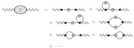
Figure 6: Ingredients of the displacement correlator. All the diagrams up to one-loop approximation are shown. These diagrams are resummed in CLPT.

The corresponding function of this Figure is given by

$$\tilde{\varLambda}_{ij}(\bm{k})=-L^{(1)}_{i}(\bm{k})L^{(1)}_{j}(\bm{k})P_{\rm L}(k)\\ -\int\frac{d^{3}p}{(2\pi)^{3}}L^{(1)}_{(i}(\bm{k})L^{(3)}_{j)}(\bm{k},\bm{p},-\bm{p})P_{\rm L}(p)P_{\rm L}(k)\\ -\frac{1}{2}\int_{\bm{k}_{12}=\bm{k}}L^{(2)}_{i}(\bm{k}_{1},\bm{k}_{2})L^{(2)}_{j}(\bm{k}_{1},\bm{k}_{2})P_{\rm L}(k_{1})P_{\rm L}(k_{2})\\ -L^{(1)}_{(i}(\bm{k})\int_{\bm{k}_{12}=\bm{k}}L^{(2)}_{j)}(\bm{k}_{1},\bm{k}_{2})B_{\rm L}(k,k_{1},k_{2}).$$ (89)

The indices $i,j$ are symmetrized on RHS of the above equation. This function is the same as $C_{ij}(\bm{k})$ in Ref. mat08b , and $-C_{ij}(\bm{k})$ in Ref. mat08a . We refer to the graph of Fig. 6 and Eq. (89) as “displacement correlator” below. To the full orders, the displacement correlator $\tilde{\varLambda}_{ij}(\bm{k})$ is given by

$$\left\langle\tilde{\varPsi}_{i}(\bm{k})\tilde{\varPsi}_{j}(\bm{k}^{\prime})\right\rangle_{\rm c}=-(2\pi)^{3}\delta_{\rm D}^{3}(\bm{k}+\bm{k}^{\prime})\tilde{\varLambda}_{ij}(\bm{k}).$$ (90)

The expression of Eq. (89) is also obtained from this equation, adopting the one-loop approximation in the perturbative expansion of Eq. (9).

Using the displacement correlator, the diagrams of Fig. 5 can be represented by a convolution integral of the form

$$\sum_{n=0}^{\infty}\frac{(-1)^{n}}{n!}k_{i_{1}}\cdots k_{i_{n}}k_{j_{1}}\cdots k_{j_{n}}\int_{\bm{k}_{1\cdots n}=\bm{k}^{\prime}}\tilde{\varLambda}_{i_{1}j_{1}}(\bm{k}_{1})\cdots\tilde{\varLambda}_{i_{n}j_{n}}(\bm{k}_{n})\\ =\int d^{3}q\,e^{-i\bm{k}_{1\cdots n}\cdot\bm{q}}\exp\left[-k_{i}k_{j}\varLambda_{ij}(\bm{q})\right],$$ (91)

where $\bm{k}$ is the wave vector of the nonlinear power spectrum $P_{XY}(\bm{k})$ to evaluate, $\bm{k}_{1\cdots n}=\bm{k}_{1}+\cdots\bm{k}_{n}$ is the total wave vector that flows through the resummed part of Fig. 5, and

$$\varLambda_{ij}(\bm{q})=\int\frac{d^{3}k}{(2\pi)^{3}}e^{i\bm{k}\cdot\bm{q}}\tilde{\varLambda}_{ij}(\bm{k})$$ (92)

is the displacement correlator in configuration space. The convolution integral of Eq. (91) contributes multiplicatively to the evaluation of the power spectrum $P_{XY}(\bm{k})$.

The displacement correlator in configuration space, Eq. (92), is given by the full-order displacement field $\bm{\varPsi}(\bm{q})$ as

$$\varLambda_{ij}(\bm{q})=-\left\langle\varPsi_{i}(\bm{q}_{2})\varPsi_{j}(\bm{q}_{1})\right\rangle_{\rm c},$$ (93)

where $\bm{q}=\bm{q}_{2}-\bm{q}_{1}$. This function is denoted as $C_{ij}(\bm{q})/2$ in Ref. CRW13 , and thus we have a correspondence,

$$C^{\rm CLPT}_{ij}(\bm{q})=2\varLambda_{ij}(\bm{q})$$ (94)

In the CLPT, the vertex resummation factor is included in a function $A_{ij}(\bm{q})=B_{ij}+C_{ij}(\bm{q})$ of their notation, where $B_{ij}=2\sigma_{\eta}^{2}\delta_{ij}$ and $\sigma_{\eta}^{2}=\langle|\bm{\varPsi}|^{2}\rangle/3$. Thus we have a correspondence,

$$A^{\rm CLPT}_{ij}(\bm{q})=\frac{2}{3}\sigma_{\eta}^{2}\delta_{ij}+2\varLambda_{ij}(\bm{q}).$$ (95)

The first term in the LHS corresponds to the vertex resummation in iPT, and is kept exponentiated in both original LRT and CLPT. The second term is kept exponentiated in CLPT and expanded in the original LRT formalism.

When the Lagrangian local bias is assumed ($c^{(1)}_{X}=\langle F^{\prime}\rangle$, $c^{(2)}_{X}=\langle F^{\prime\prime}\rangle$,…), and the convolution resummation of Fig. 5 is taken into account in the iPT, the formalism of CLPT is exactly reproduced. When the Lagrangian nonlocal bias is allowed in the iPT with the convolution resummation, we obtain a natural extension of the CLPT without restricting to models of local Lagrangian bias.

Extending this diagrammatic understanding of CLPT in the framework of iPT, it is possible to consider further convolution resummations that are not included in the formulation of CLPT. In the CLPT, only connected diagrams with two wavy lines (i.e., Fig. 6) are resummed. We define the three-point correlator of displacement, $\tilde{\varLambda}_{ijk}(\bm{k}_{1},\bm{k}_{2},\bm{k}_{3})$ where $\bm{k}_{1}+\bm{k}_{2}+\bm{k}_{3}=\bm{0}$ by the connected diagrams with three wavy lines as shown in Fig. 7.

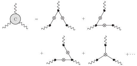
Figure 7: Connected diagrams with three wavy lines up to tree-level approximation. These diagrams are not resummed in CLPT.

This function is given by

$$\left\langle\tilde{\varPsi}_{i}(\bm{k}_{1})\tilde{\varPsi}_{j}(\bm{k}_{2})\tilde{\varPsi}_{j}(\bm{k}_{3})\right\rangle_{\rm c}\\ =-i\,(2\pi)^{3}\delta_{\rm D}^{3}(\bm{k}_{1}+\bm{k}_{2}+\bm{k}_{3})\tilde{\varLambda}_{ijk}(\bm{k}_{1},\bm{k}_{2},\bm{k}_{3}).$$ (96)

to the full order. This three-point correlator $\tilde{\varLambda}_{ijk}$ is the same as $-C_{ijk}$ in Ref. mat08b and $-iC_{ijk}$ in Ref. mat08a . In a similar way as Fig. 5 and Eq. (91), including resummations of the three-point correlator modifies the convolution integral of Eq. (91) as

$$\int d^{3}q\,e^{-i\bm{k}^{\prime}\cdot\bm{q}}\exp\left[-k_{i}k_{j}\varLambda_{ij}(\bm{q})+k_{i}k_{j}k_{k}\varLambda_{ijk}(\bm{q})\right],$$ (97)

where $\bm{k}^{\prime}$ is the total wave vector that flows through the resummed part, and

$$\varLambda_{ijk}(\bm{q})=\int\frac{d^{3}k}{(2\pi)^{3}}e^{i\bm{k}\cdot\bm{q}}\int\frac{d^{3}p}{(2\pi)^{3}}\tilde{\varLambda}_{ijk}(\bm{k},-\bm{p},\bm{p}-\bm{k}).$$ (98)

One can similarly consider four- and higher-point convolution resummations, which naturally arise in two- or higher-loop approximations. However, it is not obvious whether or not progressively including such kinds of convolution resummations actually improves the description of the strongly nonlinear regime. Comparisons with numerical simulations are necessary to check. Detailed analysis of this type of extensions in the iPT is beyond the scope of this paper, and can be considered as an interesting subject for future work.

IV.4 Renormalized perturbation theory

Recent progress in improving the standard perturbation theory (SPT) was triggered by a proposition of the renormalized perturbation theory (RPT) CS06a ; CS06b . Although this theory is formulated in Eulerian space, there are many common features with iPT in which resummations in terms of Lagrangian picture play an important role. Below, we briefly discuss these common features. However, one should note that purposes of developing RPT and iPT are not the same. The RPT formalism mainly focuses on describing nonlinear evolutions of density and velocity fields of matter, extrapolating the perturbation theory in Eulerian space. The iPT formalism mainly focuses on consistently including biasing and redshift-space distortions into the perturbation theory from the first principle as possible. The RPT (and its variants) is properly applicable only to unbiased matter clustering in real space (even though there are phenomenological approaches with freely fitting parameters, such as the model of Ref. TNB13 , for example). Thus, the resummation methods in RPT can be compared only with a degraded version of iPT without biasing and redshift-space distortions.

IV.4.1 Propagators in high-$k$ limit

An important ingredient of RPT is an interpolation scheme between low-$k$ and high-$k$ limits of the multi-point propagator of mass $\varGamma^{(n)}_{\rm m}(\bm{k}_{1},\ldots,\bm{k}_{n})$ with $\bm{k}=\bm{k}_{1\cdots n}$. Based on the Eulerian picture of perturbation theory, the high-$k$ limit of the propagator is analytically evaluated as CS06b ; BCS08

$$\varGamma^{(n)}_{\rm m}(\bm{k}_{1},\ldots,\bm{k}_{n})\approx\exp\left(-\frac{1}{2}k^{2}{\sigma_{\rm d}}^{2}\right)F_{n}(\bm{k}_{1},\ldots,\bm{k}_{n}),$$ (99)

in the fastest growing mode of density field, where

$${\sigma_{\rm d}}^{2}=\frac{1}{6\pi^{2}}\int dk^{\prime}\,P_{\rm L}(k^{\prime}),$$ (100)

$F_{n}$ is the $n$th-order kernel function of SPT, and $k=|\bm{k}_{1\cdots n}|$. Although decaying modes and the velocity sector are also included in the original RPT formalism CS06a ; CS06b , we neglect them for our purpose of comparison between RPT and iPT.

The multi-point propagator in the iPT has the form of Eqs. (5) and (6) with full orders of perturbations. In the unbiased case, $X={\rm m}$, we have

$$\varGamma^{(n)}_{\rm m}(\bm{k}_{1},\ldots,\bm{k}_{n})=\varPi(k)\hat{\varGamma}^{(n)}_{\rm m}(\bm{k}_{1},\ldots,\bm{k}_{n}),$$ (101)

where $\varPi(k)=\langle e^{-i\bm{k}\cdot\bm{\varPsi}}\rangle$ is the vertex resummation factor. The Eq. (101) should also have the same high-$k$ limit as Eq. (99), since we are dealing with the same quantities. Although explicitly proving this property in the framework of iPT is beyond the scope of this paper, a natural expectation arises that the high-$k$ limit of the resummation factor $\varPi(k)$ is given by the exponential prefactor of Eq. (99), as discussed below.

In the high-$k$ limit, the factor $e^{-i\bm{k}\cdot\bm{\varPsi}}$ which is averaged over in the resummation factor strongly oscillates as a function of displacement field $\bm{\varPsi}$. Consequently, large values of the displacement field do not contribute to the statistical average, and dominant contributions come from a regime $|\bm{\varPsi}|\lesssim k^{-1}$. In the high-$k$ limit, this condition corresponds to a weak field limit of the displacement field, which is well described by the Zel’dovich approximation, $\tilde{\bm{\varPsi}}(\bm{k})\approx(i\bm{k}/k^{2})\delta_{\rm L}(\bm{k})$. Assuming a Gaussian initial condition, higher-order cumulants of displacement field in the Zel’dovich approximation are absent in Eq. (6). Since $\langle\varPsi_{i}\varPsi_{j}\rangle_{\rm c}=\delta_{ij}\langle|\bm{\varPsi}|^{2}\rangle/3$ from rotational symmetry in real space, we have $\langle(\bm{k}\cdot\bm{\varPsi})^{2}\rangle_{\rm c}=k^{2}\langle|\bm{\varPsi}|^{2}\rangle/3=k^{2}{\sigma_{\rm d}}^{2}$ in the Zel’dovich approximation. Thus we naturally expect

$$\varPi(k)=\left\langle e^{-i\bm{k}\cdot\bm{\varPsi}}\right\rangle\approx\exp\left(-\frac{1}{2}k^{2}{\sigma_{\rm d}}^{2}\right),$$ (102)

in the high-$k$ limit, which agrees with the exponential prefactor of Eq. (99).

Assuming that the above expectation is correct, Eqs. (99) and (101) suggests the high-$k$ limit of normalized propagator is given by

$$\hat{\varGamma}^{(n)}_{\rm m}(\bm{k}_{1},\cdots,\bm{k}_{n})\approx F_{n}(\bm{k}_{1},\cdots,\bm{k}_{n}),$$ (103)

i.e., the high-$k$ limit of the normalized propagator is given by tree diagrams, and contributions from whole loop corrections are subdominant. This is a nontrivial statement, since the normalized propagator contains non-zero loop corrections in each order. For example, taking the limit $k\rightarrow\infty$ in Eq. (37) of the one-loop approximation, we have

$$\hat{\varGamma}^{(1)}_{\rm m}(k)\approx 1+\frac{58}{315}\int_{0}^{\infty}\frac{p^{2}dp}{2\pi^{2}}P_{\rm L}(p),$$ (104)

which is apparently different from $F_{1}=1$. Actually the integral in the RHS is logarithmically divergent for a spectrum of cold-dark-matter type, which has an asymptote $P_{\rm L}(k)\propto k^{-3}$ for $k\rightarrow\infty$. Thus Eq. (103) does not apparently hold when the loop corrections are truncated at any order. Thus, Eq. (103) has a highly non-perturbative nature. This situation is natural, because the high-$k$ limit of Eq. (102) is also highly non-perturbative. When the equation is truncated at any order, a high-$k$ limit gives divergent terms, while the whole factor approaches to zero. The same is true for the high-$k$ limit in the RPT formalism, Eq. (99). Provided that Eq. (99) is true, Eqs. (102) and (103) are the same statement because of Eq. (101), which is a definition of the normalized propagator.

The above argument is readily generalized in the case of non-Gaussian initial conditions. In the high-$k$ limit of the RPT formalism, the exponential factor in Eq. (99) is replaced by BCS10

$$\exp\left(-\frac{1}{2}k^{2}{\sigma_{\rm d}}^{2}\right)\rightarrow\left\langle e^{i\alpha(k)}\right\rangle=\exp\left(\sum_{n=2}^{\infty}\frac{i^{n}}{n!}\left\langle\left[\alpha(k)\right]^{n}\right\rangle_{\rm c}\right),$$ (105)

where

$$\alpha(k)\equiv-i\int\frac{d^{3}p}{(2\pi)^{3}}\frac{\bm{k}\cdot\bm{p}}{p^{2}}\delta_{\rm L}(\bm{p}).$$ (106)

Comparing these equations of RPT with Eqs. (6), (9) of iPT, there are correspondences,

$$\alpha(k) =-i\bm{k}\cdot\int\frac{d^{3}p}{(2\pi)^{3}}\bm{L}^{(1)}(\bm{p})\delta_{\rm L}(\bm{p})=-\bm{k}\cdot\bm{\varPsi}^{(1)},$$ (107)

$$\left\langle e^{i\alpha(k)}\right\rangle =\left\langle e^{-i\bm{k}\cdot\bm{\varPsi}^{(1)}}\right\rangle,$$ (108)

where $\bm{\varPsi}^{(1)}$ is the linear displacement field in configuration space at the origin. Since Eq. (101) holds in non-Gaussian initial conditions as well, the high-$k$ limit of iPT, Eq. (102), is replaced by

$$\varPi(k)\approx\left\langle e^{-i\bm{k}\cdot\bm{\varPsi}^{(1)}}\right\rangle=\exp\left[\sum_{n=2}^{\infty}\frac{(-i)^{n}}{n!}\left\langle\left(\bm{k}\cdot\bm{\varPsi}^{(1)}\right)^{n}\right\rangle_{\rm c}\right],$$ (109)

which agrees with the the replacement of RPT, Eq. (105). Since only the exponential factor is replaced in Eqs. (99) and (102), the high-$k$ limit of Eq. (103) does not change even in the case of non-Gaussian initial conditions.

IV.4.2 Nonlinear interpolation I: RegPT

In the RPT formalism, the nonlinear propagator is approximated by analytically interpolating the behaviors in the high-$k$ limit and the low-$k$ limit CS06b ; BCS08 ; CSB12 . There are at least two prescriptions for the interpolation. An interpolation scheme of Refs. BCS12 ; TBNC12 ; TNB13 , which is called RegPT, uses an prescription for the multi-point propagator truncated at the $N$-loop order as

$$\varGamma^{(n)}_{\rm RegPT}=\left(F_{n}+\delta\varGamma^{(n)}_{\rm 1\mathchar 45\relax loop}+\delta\varGamma^{(n)}_{\rm 2\mathchar 45\relax loop}+\cdots+\delta\varGamma^{(n)}_{N{\rm\mathchar 45\relax loop}}+{\rm C.T.}\right)\\ \times\exp\left(-\frac{1}{2}k^{2}{\sigma_{\rm d}}^{2}\right)$$ (110)

where $\delta\varGamma^{(n)}_{M{\rm\mathchar 45\relax loop}}$ is the $M$-loop correction term of the propagator, and ${\rm C.T.}$ is a counterterm to match the $N$-loop expression is exact in both limits, i.e.,

$${\rm C.T.}=\left[\frac{1}{2}k^{2}{\sigma_{\rm d}}^{2}+\frac{1}{8}k^{4}{\sigma_{\rm d}}^{4}+\cdots+\frac{1}{N!}\left(\frac{k^{2}{\sigma_{\rm d}}^{2}}{2}\right)^{N}\right]F_{n}\\ +\left[\frac{1}{2}k^{2}{\sigma_{\rm d}}^{2}+\cdots+\frac{1}{(N-1)!}\left(\frac{k^{2}{\sigma_{\rm d}}^{2}}{2}\right)^{N-1}\right]\delta\varGamma^{(n)}_{\rm 1\mathchar 45\relax loop}\\ +\cdots+\frac{1}{2}k^{2}{\sigma_{\rm d}}^{2}\,\delta\varGamma^{(n)}_{(N-1){\rm\mathchar 45\relax loop}}.$$ (111)

The tree-level multi-point propagators are the same as the kernel functions in SPT, i.e., $\varGamma^{(n)}_{\rm tree}=F_{n}$. It is apparent that Eq. (110) has the correct low-$k$ limit. In the high-$k$ limit, we have $\delta\varGamma^{(n)}_{M{\rm\mathchar 45\relax loop}}\approx(-k^{2}\sigma_{\rm d}^{2}/2)^{M}F_{n}/M!$ according to Eq. (99). In this limit, it can be shown by induction that all the loop corrections in the first parentheses of Eq. (110) including the counter term remarkably cancel each other, leaving only the tree-level contribution $F_{n}$. Thus Eq. (110) also has the correct high-$k$ limit, $\varGamma^{(n)}_{\rm RegPT}\rightarrow F_{n}\exp(-k^{2}{\sigma_{\rm d}}^{2}/2)$ for $k\rightarrow\infty$. The RegPT prescription of Eq. (110) can be re-expressed in a more compact form including the counterterm as

$$\varGamma^{(n)}_{\rm RegPT}=\left.\left[\exp\left(\frac{1}{2}k^{2}{\sigma_{\rm d}}^{2}\right)\,\sum_{N=0}^{\infty}\delta\varGamma^{(n)}_{N{\rm\mathchar 45\relax loop}}\right]\right|_{\rm truncated}\\ \times\exp\left(-\frac{1}{2}k^{2}{\sigma_{\rm d}}^{2}\right),$$ (112)

where $\delta\varGamma^{(n)}_{\rm 0\mathchar 45\relax loop}\equiv F_{n}$, and $[\cdots]|_{\rm truncated}$ indicates a truncation up to a given order after completely expanding the exponential factor.

The RegPT prescription of Eq. (110) can be compared with Eq. (101) in the iPT formalism. On one hand, applying a Taylor expansion of the resummation factor $\varPi$ and truncating at the $n$-loop order give the same result as the $n$-loop SPT. On the other hand, the lowest-order approximation of the resummation factor is given by Eq. (35) in real space, i.e.,

$$\varPi(k)\approx\exp\left(-\frac{1}{2}k^{2}{\sigma_{\rm d}}^{2}\right),\quad(k\rightarrow 0),$$ (113)

which is accidentally the same as the exponential factor in the high-$k$ limit of Eq. (99). From these observations, it is now clear that the RegPT prescription of Eq. (110) is equivalent to evaluate the unbiased propagator $\varGamma^{(n)}_{\rm m}$ by Eq. (101) in the framework of iPT, keeping only the lowest-order term in the vertex resummation factor $\varPi(k)$ and expanding all the other higher-order terms from the exponent. In other words, the RegPT prescription is equivalent to the restricted iPT formalism where the vertex resummations are truncated at the one-loop level (without biasing and redshift-space distortions).

IV.4.3 Nonlinear interpolation II: MPTbreeze

There is another scheme of interpolating the nonlinear propagators called MPTbreeze CSB12 , which is originally employed in the two-point propagator in the RPT formalism CS06b . This method is simpler than the RegPT, in a sense that calculations of interpolated propagators require only one-loop integrals. In the MPTbreeze prescription, the interpolated propagators are given by

$$\varGamma^{(n)}_{\rm MPTbreeze}(\bm{k}_{1},\cdots,\bm{k}_{n})=F_{n}(\bm{k}_{1},\cdots,\bm{k}_{n})\exp\left[\delta\varGamma^{(1)}_{\rm 1\mathchar 45\relax loop}(k)\right],$$ (114)

where the one-loop correction term of two-point propagator in the growing mode is explicitly given by

$$\delta\varGamma^{(1)}_{\rm 1\mathchar 45\relax loop}(k)=\int\frac{d^{3}q}{(2\pi)^{3}}\frac{P_{\rm L}(q)}{504k^{3}q^{5}}\Biggl{[}6k^{7}q-79k^{5}q^{3}+50q^{5}k^{3}\\ -21kq^{7}+\frac{3}{4}(k^{2}-q^{2})^{3}(2k^{2}+7q^{2})\ln\frac{|k-q|^{2}}{|k+q|^{2}}\Biggr{]}.$$ (115)

The notations $P_{0}(k)$, $f(k)$ $\varGamma^{(n)}_{\delta}$ in Ref. CSB12 are related to our notations by $P_{\rm L}(k)=(2\pi)^{3}D_{+}^{2}(z)P_{0}(k)$, $\delta\varGamma^{(1)}_{\rm 1\mathchar 45\relax loop}(k)=D_{+}^{2}(z)f(k)$ and $\varGamma^{(n)}_{\rm MPTbreeze}=\varGamma^{(n)}_{\delta}/D_{+}^{n}(z)$, where $D_{+}(z)$ is the linear growth factor. Since $\delta\varGamma^{(1)}_{\rm 1\mathchar 45\relax loop}(k)\rightarrow-k^{2}{\sigma_{\rm d}}^{2}/2$ in the high-$k$ limit and $\delta\varGamma^{(1)}_{\rm 1\mathchar 45\relax loop}(k)\rightarrow 0$ in the low-$k$ limit, Eq. (114) has correct limits.

It is worth noting that the prescription of Eq. (114) corresponds to replacing all the loop-correction terms of propagators by

$$\delta\varGamma^{(n)}_{N{\rm\mathchar 45\relax loop}}(\bm{k}_{1},\ldots,\bm{k}_{n})\rightarrow\frac{1}{N!}\left[\delta\varGamma^{(1)}_{\rm 1\mathchar 45\relax loop}(k)\right]^{N}F_{n}(\bm{k}_{1},\ldots,\bm{k}_{n}).$$ (116)

Both prescriptions of MPTbreeze and RegPT give similar results, and they agree with numerical simulations fairly well in the mildly nonlinear regime CSB12 ; TBNC12 . Thus the approximation of Eq. (116) turns out to be empirically good, although the physical origin of the goodness in this prescription is somehow unclear.

According to Eq. (37) or Eq. (38), the iPT-normalized two-point propagator of mass is related to the function $\delta\varGamma^{(1)}_{\rm 1\mathchar 45\relax loop}(k)$ by

$$\delta\varGamma^{(1)}_{\rm 1\mathchar 45\relax loop}(k)=\delta\hat{\varGamma}^{(1)}_{\rm 1\mathchar 45\relax loop}(k)-\frac{1}{2}k^{2}{\sigma_{\rm d}}^{2},$$ (117)

where $\delta\hat{\varGamma}^{(1)}_{\rm 1\mathchar 45\relax loop}$ is the one-loop correction term which corresponds to the integral in Eq. (38) without bias, $c^{(n)}_{X}=0$, or

$$\delta\hat{\varGamma}^{(1)}_{\rm 1\mathchar 45\relax loop}(k)=\frac{5}{21}R_{1}(k)+\frac{3}{7}R_{2}(k),$$ (118)

as seen in Eq. (58). Substituting Eq. (117) into Eq. (114), we have

$$\varGamma^{(n)}_{\rm MPTbreeze}=F_{n}\,\exp\left[{\delta\hat{\varGamma}^{(1)}_{\rm 1\mathchar 45\relax loop}(k)}\right]\,\exp\left(-\frac{1}{2}k^{2}{\sigma_{\rm d}}^{2}\right).$$ (119)

Comparing this form with Eq. (112), the relation between the prescriptions of RegPT and MPTbreeze is explicit. Both prescriptions differ in the prefactor preceding to the exponential damping factor; a truncation scheme is employed in RegPT, and a simple model of the higher-loop corrections is employed in MPTbreeze.

V Conclusions

The iPT is a unique theory of cosmological perturbations to predict the observable spectra of biased tracers both in real space and in redshift space. This theory does not have phenomenological free parameter once the bias model is fixed. In other words, all the uncertainties regarding biasing are packed into the renormalized bias functions $c_{X}^{(n)}$, and weakly nonlinear gravitational evolutions of spatial clustering of biased tracers are described by iPT without any ambiguity. In this way, the iPT separates the bias uncertainties from weakly nonlinear evolutions of spatial clustering. The renormalized bias functions are evaluated for a given model of bias.

Most of physical models of bias, such as the halo bias and peaks bias, fall into the category of the Lagrangian bias. Redshift-space distortions are simpler to describe in Lagrangian picture than in Eulerian picture. The iPT is primarily based on the Lagrangian picture of perturbations, and therefore effects of Lagrangian bias and redshift-space distortions are naturally incorporated in the framework of iPT.

In this paper, general expressions of the one-loop power spectra calculated from the iPT are presented for the first time. The cross power spectra of differently biased objects, $P_{XY}(\bm{k})$, both in real space and in redshift space are explicitly given in terms of two-dimensional integrals at most up to one-loop order. The final result in real space is given by Eq. (47) with Eqs. (35), (42), (43), (44), and that in redshift space is given by Eq. (71) with Eqs. (57), (59), (60) and (70). When the vertex resummation is not preferred, one can alternatively use Eq. (36) instead of Eq. (35). An example of the renormalized bias functions is given by Eq. (19) for a simple model of halo bias.

The iPT is a nontrivial generalization of the method of Ref. mat08b , which is applicable only to the case that the Lagrangian bias is local and that the initial condition is Gaussian. Although the derivations are quite different from each other, it is explicitly shown that the general iPT expression of the power spectrum exactly reduces to the expression of Ref. mat08b in models of local Lagrangian bias and Gaussian initial condition.

The effects of primordial non-Gaussianity are included as well. The consequent results are consistent with those derived by popular method of peak-background split. In fact, the iPT provides more accurate evaluations of the scale-dependent bias due to the primordial non-Gaussianity mat12 . In the present paper, both effects of gravitational nonlinearity and primordial non-Gaussianity are simultaneously included in an expression of biased power spectrum. Thus, the most general expressions of power spectrum with leading-order (one-loop) nonlinearity and non-Gaussianity are newly obtained in this paper.

In this paper, comparisons of the analytic expressions with numerical $N$-body simulations are quite limited. In an accompanying paper SM13 , the results in the present paper are used in calculating the nonlinear auto- and cross-correlation functions of halos and mass, and are compared with numerical simulations, focusing on stochastic properties of bias. We have confirmed that effects of nonlocal bias is small in the weakly nonlinear regime for the Gaussian initial conditions. That is not surprising because nonlocality in the halo bias is effective on scales of the halo mass indicated by Eq. (22); for example, $R\simeq 0.7$, $1.4$, $3.1$, $6.6\,h^{-1}{\rm Mpc}$ for $M=10^{11}$, $10^{12}$, $10^{13}$, $10^{14}h^{-1}M_{\odot}$, respectively, while one-loop perturbation theory is applicable on scales $\gg 5$–$10\,h^{-1}{\rm Mpc}$ for $z\lesssim 3$. Therefore, the predictions of iPT in Gaussian initial conditions with one-loop approximation are almost the same as those of LRT with Lagrangian local bias mat08a , which have been compared in detail SM11 with numerical simulations of halos both in real space and in redshift space. The nonlocality of halo bias should be important on small scales, and further investigations on the renormalized bias functions are interesting extension of the present work.

In the framework of iPT, the vertex resummation is naturally defined, resulting in the resummation factor $\varPi(\bm{k})$ of Eq. (35) in real space or Eq. (57) in redshift space. The vertex resummation of iPT is closely related to other resummation methods like RPT which are formulated in Eulerian space. When the vertex resummation is truncated up to one-loop order, the iPT without bias and redshift-space distortions gives the equivalent formalism to the RegPT, a version of RPT with regularized multi-point propagators.

Beyond the vertex resummations, the scheme of CLPT is readily applied to the framework of iPT as discussed in Sec. IV.3. Further resummation scheme of convolution can be also considered. It might be an interesting application of iPT to include those type of further resummations in the presence of nonlocal bias and redshift-space distortions.

Although the resummation technique has proven to be useful in the one-loop approximation, it is not trivial whether the same is true in arbitrary orders. The vertex resummation is not compulsory in iPT, rather it is optional. The general form of vertex resummation factor in iPT is given by Eq. (6). When this exponential function is expanded into polynomials, we obtain a perturbative expression of power spectrum without resummation, which is an analogue to SPT. However, for evaluations of the correlation function, the exponential damping of the resummation factor stabilizes the numerical integrations of Fourier transform, and therefore the vertex resummation is preferred.

The nonlocal model of halo bias mat12 explained in Sec. II.2 is still primitive. There are plenty of rooms to improve the model of nonlocal bias in future work. The iPT provides a natural framework to separate tractable problems of weakly nonlinear evolutions of biased tracers from difficult problems of fully nonlinear phenomena of biasing.

Appendix A Diagrammatic rules

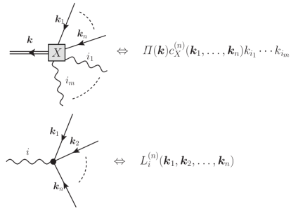
Figure 8: Diagrammatic rules of iPT: dynamics and biasing.

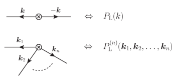
Figure 9: Diagrammatic rules of iPT: primordial spectra.

A set of diagrammatic rules in iPT which is used in this paper is summarized in this Appendix. Full set of rules and their derivations are found in Ref. mat11 . The relevant diagrammatic rules are shown in Fig. 8 and 9. Physical meanings of the graphs are as follows: a double solid line corresponds to the number density field $\delta_{X}(\bm{k})$, a square box represents partial resummations of dynamics and biasing, a wavy line represents the displacement field, a black dot represents nonlinear evolutions of the displacement field, a crossed circle represents the primordial spectra. The procedures for obtaining a cross polyspectra $P^{(N)}_{X_{1}\cdots X_{N}}(\bm{k}_{1},\ldots,\bm{k}_{N})$ of different types of objects $X_{1},\ldots,X_{N}$ are listed below. Auto polyspectra are obtained by just setting $X_{1}=\cdots=X_{N}$. The power spectrum is a special case of polyspectra with $N=2$.

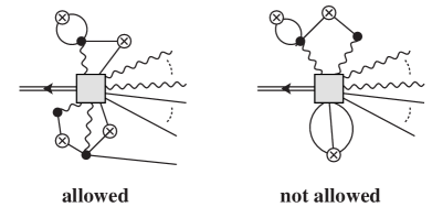
Figure 10: Examples of external vertex which is allowed (left) and not allowed (right) in iPT.

1. Draw $N$ square boxes with labels $X_{i}$ ($i=1,\ldots N$), each of which has a double solid line. Label each double solid line with an outgoing wavevector that corresponds to an argument of the polyspectra $P^{(N)}_{X_{1}\cdots X_{N}}$.

2. Consider possible ways to connect all the square boxes by using wavy lines, solid lines, black dots and crossed circles, satisfying following constraints:

   1. An end of a wavy line should be connected to a square box, and the other end should be connected to a black dot.

   2. An end of a solid line should be connected to a crossed circle, and the other end should be connected to either a square box or a black dot.

   3. Only one wavy line can be attached to a black dot while arbitrary number of solid line(s) can be attached to a black dot.

   4. A piece of graph which is connected to a single square box with only wavy lines or with only solid lines is not allowed.

3. Label each (solid and wavy) line with a wavevector and its direction. The wavevectors should be conserved at each vertex of square box, black dot, and crossed circle. Label each wavy line with spatial index together with a wavevector.

4. Apply the diagrammatic rules of Figs. 8 and 9 to every distinct graphs.

5. Integrate over wavevectors as $\int d^{3}k_{i}^{\prime}/(2\pi)^{3}$, where $\bm{k}_{i}^{\prime}$ are not determined by constraints of wavevector conservation at vertices.

6. When there are $m$ equivalent pieces in a graph, put a statistical factor $1/m!$ for each set of equivalent pieces.

7. Sum up all the contributions from every distinct graphs up to necessary orders of perturbations.

The rule 2.-(d) is due to partial resummations of the square box. For example, the left diagram of Fig. 10 is allowed. There is a piece of graph that is connected to a single square box with both wavy and solid lines. However, the right diagram of Fig. 10 is not allowed, because of double reasons. One is that the upper piece of graph is connected to a single square box with only wavy lines. The other is that the lower piece of graph with only solid lines connected to a single square box. Each reason itself prohibits this diagram from counted.

References

• (1) D. J. Eisenstein, W. Hu, and M. Tegmark, Astrophys. J. Letters, 504, L57 (1998).
• (2) T. Matsubara, Astrophys. J., 615, 573 (2004).
• (3) D. J. Eisenstein et al., Astrophys. J., 633, 560 (2005).
• (4) N. Dalal, O. Doré, D. Huterer and A. Shirokov, Phys. Rev. D77, 123514 (2008).
• (5) S. Matarrese and L. Verde, Astrophys. J. Letters, , 677, L77 (2008).
• (6) A. Slosar, C. Hirata, U. Seljak, S. Ho, N. Padmanabhan, J. Cosmol. Astropart. Phys., 8, 31 (2008).
• (7) A. Taruya, K. Koyama and T. Matsubara, Phys. Rev. D78, 123534 (2008).
• (8) V. Desjacques, U. Seljak and I. T. Iliev, Mon. Not. R. Astron. Soc., 396, 85 (2009).
• (9) K. S. Dawson et al., Astron. J., 145, 10 (2013).
• (10) http://www.kusastro.kyoto-u.ac.jp/Fastsound/
• (11) D. Schlegel et al., arXiv:1106.1706 (2011).
• (12) LSST Science Collaborations: P. A. Abell, et al., arXiv:0912.0201 (2009).
• (13) R. Ellis et al., arXiv:1206.0737 (2012).
• (14) http://www.darkenergysurvey.org/
• (15) R. Laureijs et al., arXiv:1110.3193 (2011).
• (16) A. F. Heavens, S. Matarrese, and L. Verde, Mon. Not. R. Astron. Soc., 301, 797 (1998).
• (17) R. Scoccimarro, H. M. P. Couchman, and J. A. Frieman, Astrophys. J., 517, 531 (1999)
• (18) A. Taruya, Astrophys. J., 537, 37 (2000).
• (19) P. McDonald, Phys. Rev. D74, 103512 (2006); 74, 129901(E) (2006).
• (20) D. Jeong and E. Komatsu, Astrophys. J., 691, 569 (2009).
• (21) T. Matsubara, Phys. Rev. D83, 083518 (2011).
• (22) T. Matsubara, Phys. Rev. D77, 063530 (2008).
• (23) T. Matsubara, Phys. Rev. D78, 083519 (2008); 78, 109901(E) (2008)
• (24) T. Okamura, T., A. Taruya and T. Matsubara, arXiv:1105.1491
• (25) M. Sato and T. Matsubara, Phys. Rev. D84, 043501 (2011).
• (26) W. H. Press and P. Schechter, Astrophys. J., 187, 425 (1974).
• (27) J. R. Bond, S. Cole, G. Efstathiou, and N. Kaiser, Astrophys. J., 379, 440 (1991).
• (28) H. J. Mo and S. D. M. White, Mon. Not. R. Astron. Soc., 282, 347 (1996).
• (29) H. J. Mo, Y. P. Jing, and S. D. M. White, Mon. Not. R. Astron. Soc., 284, 189 (1997).
• (30) R. K. Sheth and G. Tormen, Mon. Not. R. Astron. Soc., 308, 119 (1999).
• (31) R. Scoccimarro, R. K. Sheth, L. Hui, and B. Jain, Astrophys. J., 546, 20 (2001).
• (32) A. Cooray and R. Sheth, Phys. Rep., 372, 1 (2002).
• (33) K. C. Chan, R. Scoccimarro and R. K. Sheth, Phys. Rev. D85, 083509 (2012).
• (34) K. C. Chan and R. Scoccimarro, Phys. Rev. D86, 103519 (2012).
• (35) R. K. Sheth, K. C. Chan and R. Scoccimarro, arXiv:1207.7117 (2012).
• (36) T. Matsubara, Phys. Rev. D86, 063518 (2012).
• (37) T. Buchert, Astron. Astrophys., 223, 9 (1989).
• (38) F. Moutarde, J.-M. Alimi, F. R. Bouchet, R. Pellat, and A. Ramani, Astrophys. J., 382, 377 (1991).
• (39) T. Buchert, Mon. Not. R. Astron. Soc., 254, 729 (1992). (1993).
• (40) P. Catelan, Mon. Not. R. Astron. Soc., 276, 115 (1995). R. Juszkiewicz, Astron. Astrophys., 298, 643 (1995). (1996).
• (41) C. Rampf and T. Buchert, J. Cosmol. Astropart. Phys., 6, 21 (2012).
• (42) T. Tatekawa, Progress of Theoretical and Experimental Physics, 2013, id.013E03 (2013).
• (43) T. Nishimichi, T. Matsubara, A. Taruya, in prep. M. B. Wise, Astrophys. J., 311, 6 (1986). (1994).
• (44) F. Bernardeau, S. Colombi, E. Gaztañaga, and R. Scoccimarro, Phys. Rep., 367, 1 (2002)
• (45) M. Crocce and R. Scoccimarro, Phys. Rev. D73, 063519 (2006).
• (46) M. Crocce and R. Scoccimarro, Phys. Rev. D73, 063520 (2006).
• (47) F. Bernardeau, M. Crocce and R. Scoccimarro, Phys. Rev. D78, 103521 (2008).
• (48) F. Bernardeau, M. Crocce and E. Sefusatti, Phys. Rev. D82, 083507 (2010).
• (49) F. Bernardeau, M. Crocce and R. Scoccimarro, Phys. Rev. D85, 123519 (2012).
• (50) M. Crocce, R. Scoccimarro and F. Bernardeau, Mon. Not. R. Astron. Soc., 427, 2537 (2012).
• (51) A. Taruya, F. Bernardeau, T. Nishimichi, S. Codis, Phys. Rev. D86, 103528 (2012).
• (52) A. Taruya, T. Nishimichi and F. Bernardeau, arXiv:1301.3624 (2013).
• (53) J. Carlson, B. Reid and M. White, Mon. Not. R. Astron. Soc., 429, 1674 (2013)
• (54) T. Matsubara, Astrophys. J. Suppl. Ser., 101, 1 (1995)
• (55) M. S. Warren, K. Abazajian, D. E. Holz, L. Teodoro, Astrophys. J., 646, 881 (2006).
• (56) M. Crocce, P. Fosalba, F. J. Castander and E. Gaztãnaga, Mon. Not. R. Astron. Soc., 403, 1353 (2010).
• (57) N. Kaiser Mon. Not. R. Astron. Soc., 227, 1 (1987).
• (58) A. J. S. Hamilton, The Evolving Universe, 231, 185 (1998). (astro-ph/9708102).
• (59) A. J. S. Hamilton, Astrophys. J. Letters, 385, L5 (1992).
• (60) S. Cole, K. B. Fisher and D. H. Weinberg, Mon. Not. R. Astron. Soc., 267, 785 (1994).
• (61) M. Sato and T. Matsubara, Phys. Rev. D87, 123523 (2013).
• (62) V. Springel, Mon. Not. R. Astron. Soc., , 364, 1105 (2005).
• (63) M. Crocce, S. Pueblas and R. Scoccimarro, Mon. Not. R. Astron. Soc., , 373, 369 (2006).
• (64) P. Valageas and T. Nishimichi, Astron. Astrophys., , 527, A87 (2011).
• (65) A. Lewis, A. Challinor and A. Lasenby, Astrophys. J., , 538, 473 (2000).
• (66) M. Davis, G. Efstathiou, C. S. Frenk and S. D. M. White, Astrophys. J., , 292, 371 (1985).
• (67) M. Crocce, F. J. Castander, E. Gaztanaga, P. Fosalba and J. Carretero, arXiv:1312.2013 (2013).
• (68) F. Schmidt and M. Kamionkowski, Phys. Rev. D82, 103002 (2010).
• (69) V. Desjacques, D. Jeong and F. Schmidt, Phys. Rev. D84, 061301 (2011).
• (70) V. Desjacques, D. Jeong and F. Schmidt, Phys. Rev. D84, 063512 (2011).