Niedipolowe pole magnetyczne nad czapą polarną gwiazdy neutronowej a fizyka promieniowania pulsarów

prof. dr hab. Giorgi Melikidze

Zielona Góra

Non-dipolar magnetic field at the polar cap of neutron stars and the physics of pulsar radiation

To Natalia, my daughter, and Beata, my wife, for being there…

Abstract

Despite the fact that pulsars have been observed for almost half a century, until now many questions have remained unanswered. One of the fundamental problems is describing the physics of pulsar radiation. By trying to find an answer to this fundamental question we use the analysis of X-ray observations in order to study the polar cap region of radio pulsars. The size of the hot spots implies that the magnetic field configuration just above the stellar surface differs significantly from a purely dipole one. By using the conservation of the magnetic flux we can estimate the surface magnetic field as of the order of $10^{14}\,{\rm G}$. On the other hand, the temperature of the hot spots is about a few million Kelvins. Based on these two facts the Partially Screened Gap (PSG) model was proposed to describe the Inner Acceleration Region (IAR). The PSG model assumes that the temperature of the actual polar cap is equal to the so-called critical value, i.e. the temperature at which the outflow of thermal ions from the surface screens the gap completely.

We have found that, depending on the conditions above the polar cap, the generation of high energetic photons in IAR can be caused either by Curvature Radiation (CR) or by Inverse Compton Scattering (ICS). Completely different properties of both processes result in two different scenarios of breaking the acceleration gap: the so-called PSG-off mode for the gap dominated by CR and the PSG-on mode for the gap dominated by ICS. The existence of two different mechanisms of gap breakdown naturally explains the mode-changing phenomenon. Different characteristics of plasma generated in the acceleration region for both processes also explain the pulse nulling phenomenon. Furthermore, the mode changes of the IAR may explain the anti-correlation of radio and X-ray emission in very recent observations of PSR B0943+10 (Hermsen et al.,, 2013).

Simultaneous analysis of X-ray and radio properties have allowed to develop a model which explains the drifting subpulse phenomenon. According to this model the drift takes place when the charge density in IAR differs from the Goldreich-Julian co-rotational density. The proposed model allows to verify both the radio drift parameters and X-ray efficiency of the observed pulsars.

Streszczenie

Pomimo, że pulsary są badane już od prawie pół wieku, do dzisiaj nie udało się znaleźć odpowiedzi na wiele pytań. Jednym z fundamentalnych problemów jest opis fizyki promieniowania pulsarów. Próbując znaleźć odpowiedź na to fundamentalne pytanie, wykorzystujemy analizę obserwacji rentgenowskich w celu badania obszaru czapy polarnej pulsarów. Rozmiar obserwowanych gorących plam wskazuje, że konfiguracja pola magnetycznego na powierzchni gwiazdy różni się znacznie od pola czysto dipolowego. Wykorzystując prawo zachowania strumienia magnetycznego możemy oszacować siłę pola magnetycznego w obszarze czapy polarnej, które dla obserwowanych pulsarów jest rzędu $10^{14}\,{\rm G}$. Z drugiej strony obserwowana temperatura gorącej plamy jest rzędu kilku milionów kelwinów. Opierając się na tych dwóch faktach wykorzystujemy model częściowo-ekranowanej przerwy akceleracyjnej (z ang. Partially Screened Gap - PSG), aby opisać wewnętrzną przerwę akceleracyjną (z ang. Inner Acceleration Region - IAR). Model PSG zakłada, że temperatura czapy polarnej jest bliska do tak zwanej wartości krytycznej tzn. takiej przy, której termiczny odpływ jonów z powierzchni w pełni ekranuje przerwę akceleracyjną.

W zależności od warunków jakie panują w obszarze czapy polarnej, mechanizmem odpowiedzialnym za generowanie wysokoenergetycznych fotonów w IAR może być promieniowanie krzywiznowe (z ang. Curvature Radiation - CR) lub odwrotne rozpraszanie Comptona (z ang. Inverse Compoton Scattering - ICS). Całkowicie różne właściwości obu tych procesów prowadzą do sytuacji, w której możemy wyróżnić dwa scenariusze zamknięcia przerwy akceleracyjnej: tzw. PSG-off dla przerwy zdominowanej przez promieniowanie CR, oraz tzw. PSG-on dla przerwy zdominowanej przez ICS. Istnienie dwóch różnych mechanizmów zamknięcia przerwy w naturalny sposób tłumaczy zjawisko zmiany trybu promieniowania pulsarów (z ang. mode-changing). Różna charakterystyka plazmy generowanej w obszarze akceleracyjnym dla obu tych trybów tłumaczy zjawisko sporadycznego braku pojedynczych pulsów (z ang. pulse nulling) w obserwacjach radiowych. Co więcej zmiana trybu w jakim pracuje przerwa akceleracyjna może zostać powiązana z antykorelacją promieniowania radiowego i rentgenowskiego wykazaną w ostatnich obserwacjach PSR B0943+10 (Hermsen et al.,, 2013).

Jednoczesna analiza właściwości promieniowania rentgenowskiego i radiowego pozwoliła na opracowanie modelu dryfujących składowych pulsu pojedynczego (z ang. subpulses). Model ten zakłada, że dryf jest wynikiem różnicy gęstości ładunku w IAR w stosunku do gęstości korotacji. Proponowany model pozwala zarówno na weryfikację wyznaczonych parametrów dryfu oraz na weryfikację np. efektywności promieniowania rentgenowskiego.

Introduction

The history of neutron stars began in the early 1930s when Subrahmanyan Chandrasekhar calculated the critical mass for a white dwarf. As soon as the mass of a white dwarf exceeds the critical value (e.g. due to accretion of matter from a companion star) it collapses and a neutron star is formed. Chandrasekhar estimated that the critical mass was approximately $1.4$ solar masses (${\rm M}_{\odot}$). Even before James Chadwick’s discovery of neutrons (1932), Lev Landau anticipated the existence of neutron stars by writing about stars in which “atomic nuclei come in close contact, forming one gigantic nucleus”. In 1934 Baade and Zwicky, proposed that the “supernova process represents the transition of an ordinary star into a neutron star”. Five years later Oppenheimer and Volkoff, (1939), using the work of Tolman, (1939), computed an upper bound on the mass of a star composed of neutron-degenerate matter. They assumed that the neutrons in a neutron star form a cold degenerate Fermi gas which leads to an upper bound of approximately $0.7\,{\rm M}_{\odot}$. Modern estimates of the critical mass for neutron stars range from approximately $1.5\,{\rm M}_{\odot}$ to $3\,{\rm M}_{\odot}$ (Bombaci,, 1996). This uncertainty reflects the fact that the equation of state for extremely dense matter is not well known. Let us note that the radius of a neutron star should be $R\approx 10{\rm\,km}$. On the other hand nobody expected to detect any emission from neutron stars due to their small size and the lack of theoretical predictions about any radiation processes, except for thermal radiation. Thus, it took almost forty years to detect emission from a neutron star.

The breakthrough came on 28 November 1967 with the radio observations that were performed by Jocelyn Bell-Burnell and Anthony Hewish. They observed radio pulses separated by $1.33$ seconds. The world “pulsar” was adopted to reflect the specific property of these celestial objects. The suggestion that pulsars were rotating neutron stars was put forth independently by Gold, (1968) and Pacini, (1968), and was soon proved beyond a reasonable doubt by the discovery of a pulsar with a very short ($33$-millisecond) pulse period in the Crab nebula. It was suggested that this pulsar powers the activity of the nebula (Pacini,, 1968). Nearly 2000 pulsars have been found so far. Observations of pulsars provide valuable information about neutron star physics, general relativity, the interstellar medium, celestial mechanics, planetary physics, the Galactic gravitational potential, the magnetic field and even cosmology. Studying neutron stars is therefore a very broad issue and it is beyond the scope of this thesis to describe the current status of the theory of neutron stars or pulsar population studies in detail. We rather refer the reader to the literature (Michel,, 1991; Mészáros,, 1992; Glendenning,, 1996; Weber,, 1999) and provide only a basic theoretical background that is relevant to the subject of this thesis.

Following the ideas of Pacini, (1968) and Gold, (1968) radio pulsars can be interpreted as rapidly spinning, strongly magnetised neutron stars radiating at the expense of their rotational energy. Neutron stars consist of compressed matter with density in its core exceeding nuclear density $\rho_{{\rm nuc}}=2.8\times 10^{14}{\rm\,g\,cm^{-3}}$. Direct and accurate mass measurements come from timing observations of binary pulsars and are consistent with a typically assumed neutron star mass $M\approx 1.4\,{\rm M}_{\odot}$. Most models predict a radius of $R\sim 10\,{\rm km}$, which is consistent with the theoretical upper and lower limits. However, the measurements of neutron star radii are much less reliable than the mass measurements. Therefore, the moment of inertia for these canonical values ($M=1.4\,{\rm M}_{\odot}$, $R=10{\rm\,km}$) $I\approx\left(2/5\right)MR^{2}\approx 10^{45}{\rm\,g\,cm^{2}}$ may be uncertain by $\sim 70\%$. The increase rate of a pulsar period, $\dot{P}={\rm d}P/{\rm d}t$, is related to the rate of rotational kinetic energy loss (spin-down luminosity) $\dot{E}=L_{{\rm SD}}=4\pi^{2}I\dot{P}P^{-3}$. In most cases only a tiny fraction of $\dot{E}$ can be converted into radio emission. The efficiency, $\chi_{{\rm radio}}=L_{{\rm radio}}/\dot{E}$, in the radio bands is typically in the range of $\sim 10^{-7}-10^{-5}$. It is assumed that the bulk of the rotational energy is converted into magnetic dipole radiation. The expected evolution of the angular velocity ($\Omega=2\pi/P$) of a rotating magnetic dipole can be described as $\dot{\Omega}\sim\Omega^{n}$, and the breaking index is $n=3$ for the pure dipole radiation. Indeed, the observed values of the breaking index (e.g. Becker,, 2009) confirm the above statement, e.g.: for the Crab $n=2.515\pm 0.005$, for PSR B1509-58 $n=2.8\text{$\pm$}0.2$, for PSR B0540-69 $n=2.28\text{$\pm$}0.02$, for PSR J1911-6127 $n=2.91\pm 0.05$, for PSR J1846-0258 $n=2.65\text{$\pm$}0.01$, and for the Vela pulsar $n=1.4\text{$\pm$}0.2$. On the other hand the observations of pulsar wind nebulae suggest that a significant fraction of the pulsar rotational energy is carried away by a pulsar wind. Furthermore, recent observations of high energy radiation from pulsars show that significantly more energy is radiated in the form of X-rays and $\gamma$-rays than in the form of radio emission (e.g. Abdo et al.,, 2010). Thus, pure magnetic breaking does not provide full information about the physical processes that take place in the pulsar magnetosphere.

Despite the fact that pulsars have been observed for almost half a century, many questions still remain unanswered. One of the fundamental problems concerns the physics of pulsar radiation. Radio observations alone cannot point to the model (e.g. vacuum gap, slot gap, outer gap, free outflow, etc.) that correctly describes the source of pulsar activity. Observations carried out by relatively new high-energy instruments, e.g. Chandra and XMM-Newton, significantly extended the spectra over which we can study pulsars and their environments. There is no consensus about the origin of pulsar X-ray emission (Michel,, 1991). We can distinguish two main types of models: the polar gap and the outer gap. The polar gap models suggest that the emission region is located in the vicinity of the neutron star polar caps, while the outer gap models assume that particle acceleration and X-ray emission take place close to the pulsar light cylinder. In both types of models high energy radiation is generated by relativistic particles accelerated in charge-depleted regions, while the high energy photons are emitted by means of Curvature Radiation (CR), Synchrotron Radiation (SR) and Inverse Compton Scattering (ICS). Both models are able to interpret existing observational data.

In this thesis we will use the Partially Screened Gap (PSG) model (Gil et al., 2007a, ). The PSG model assumes the existence of the Inner Acceleration Region (IAR) above the polar cap (a region penetrated by the open field lines) where the electric field has a component along the magnetic field. In this region particles (electrons and positrons) are accelerated in both directions: outward and toward the stellar surface. Consequently, outflowing particles are responsible for generation of magnetospheric emission (radio and high-frequency) while the backflowing particles heat the surface and provide the required energy for thermal emission. The PSG model is an extension of the Standard Model developed by Ruderman and Sutherland, (1975) and takes into account the thermionic ion flow from the stellar surface heated up to a high temperature (a few million Kelvins) by the backstreaming particles. In such a scenario an analysis of X-ray radiation is an excellent method of obtaining insight into the most intriguing region of the neutron star.

Chapter 1 X-ray emission from Radio Pulsars

1.1 Brief historical overview

X-ray photons can only be detected by telescopes operating at high altitudes or above the Earth’s atmosphere, thus detectors should be mounted on high-flying balloons, rockets or satellites. The first (i.e. carried out from space) X-ray observations were performed by a team led by Herbert Friedman in 1948. The team estimated the luminosity of X-ray radiation from the solar corona. They found that X-ray luminosity is weaker by a factor of $10^{6}$ than luminosity in the optical wave range. Up until the early 1960s it was widely believed that all other stars should be so faint in the X-rays that their observations would be hopeless. The situation changed in 1962 when a team led by Bruno Rossi and Riccardo Giacconi, when trying to find fluorescent X-ray photons from the moon, accidentally detected X-rays from Sco X-1. Subsequent flights launched to confirm these first results detected Tau X-1, a source in the constellation Taurus which coincided with the Crab supernova remnant (Bowyer et al.,, 1964). The search for similar sources became a source of strong motivation for the further development of X-ray astronomy.

Before the first direct detection of a neutron star by Hewish et al., (1968), it was predicted that neutron stars could be powerful sources of thermal X-ray emission due to a high surface temperature ($T_{{\rm s}}$). The expected value of the surface temperature was estimated as $T_{{\rm s}}\sim 1\,{\rm MK}$ (Chiu and Salpeter,, 1964; Tsuruta,, 1964). The first X-ray observations of isolated neutron stars were initiated by the Einstein Observatory, which was launched by NASA in 1978. Using a high-resolution imaging camera sensitive in the $0.2-3.5\,{\rm keV}$ energy range provided unprecedented levels of sensitivity (hundreds of times better than had previously been achieved). The Einstein detected X-ray emission from a number of neutron stars (mainly as compact sources in supernova remnants) such as the middle-aged radio pulsars B0656+14, B1055-52 and the old pulsar B0950+08. The Einstein observatory re-entered the Earth’s atmosphere and burned up on 25 March 1982. The next ”decade of space science” was opened in the 1990s with the launch of the ROSAT mission that was sensitive in the $0.1-2.4\,{\rm keV}$ energy range. One of the major results achieved with the ROSAT was the identification of the $\gamma$-ray source Geminga as a pulsar, hence a neutron star (Halpern and Holt,, 1992).

The current era of X-ray observations of neutron stars was begun with the launch of two satellites: the XMM-Newton owned by the European Space Agency and the Chandra owned by the National Aeronautics and Space Administration. These two grazing-incidence X-ray telescopes were placed in orbit in 1999. They were equipped with cameras and high-resolution spectrometers sensitive to low-energy X-rays: from $0.08$ to $10\,{\rm keV}$ for the Chandra and from $0.1$ to $15\,{\rm keV}$ for the XMM-Newton. While the two observatories have similar designs, they are not identical. The XMM-Newton observatory has three X-ray telescopes that provide six times the collecting area and a broader spectral range in images than the Chandra, while the Chandra has a much finer spatial resolution and a broader spectral range in its high-resolution spectroscopy than does the XMM-Newton. Both observatories are in a highly-elliptical orbit that permits continuous observations of up to 40 hours. The Chandra and XMM-Newton have greatly increased the quality and availability of observations of X-ray thermal radiation from neutron star surfaces. The total number of isolated neutron stars of different types detected in X-rays is hard to find since not all data have been published. Some authors estimate that about one hundred rotation-powered pulsars were detected in the X-rays (Zavlin, 2007a, ; Becker,, 2009).

1.2 X-ray emission from isolated neutron stars

X-ray emission is a common feature of all kinds of neutron stars. Furthermore, X-ray observations have led to the discovery of other types of neutron stars that for various reasons were missed in the standard searches for radio pulsars. These new classes, such as X-ray Dim Isolated Neutron Stars, Central Compact Objects in supernovae remnants, Anomalous X-ray Pulsars, and Soft Gamma-ray Repeaters, are only a small fraction of the whole number of observed pulsars but provide valuable information on the diversity of the neutron star population.

X-ray radiation from an isolated neutron star can in general consist of two distinguishable components: thermal and nonthermal emissions. The thermal emission can originate either from the entire surface of a cooling neutron star or from spots around the magnetic poles on the stellar surface (polar caps and adjacent areas). The temperature of a neutron star at the moment of its formation is extremely high - its value is even as high as $10^{10}-10^{11}\,{\rm K}$. Such a high initial temperature leads to very fast cooling, and after several minutes the temperature of the star interior falls to $10^{9}-10^{10}{\rm\,K}$. After $10-100\,{\rm yr}$ the neutron star will cool down to a few times $10^{6}\,{\rm K}$. At this point, depending on the still poorly known properties of super-dense matter, the temperature evolution can follow two different scenarios. The standard cooling scenario predicts that the temperature decreases gradually, down to $\sim\left(0.3-1\right)\times 10^{6}\,{\rm K}$ by the end of the neutrino cooling era and then falls exponentially to temperatures lower than $\sim 10^{5}\,{\rm K}$ in $\sim 10^{7}\,{\rm yr}$. In the accelerated cooling scenario, which implies higher central densities (up to $10^{15}\,{\rm g\,cm^{-3}}$) and/or exotic interior composition (e.g. quark plasma), at the age of $\sim 10-100\,{\rm yr}$ the temperature decreases rapidly down to $\sim\left(0.3-0.5\right)\times 10^{6}\,{\rm K}$ and is followed by a more gradual decrease down to the same $\sim 10^{5}\,{\rm K}$ in $\sim 10^{7}\,{\rm yr}$ (Becker,, 2009). The thermal evolution of neutron stars is very sensitive to the composition (and structure) of their interiors, therefore, measuring surface temperatures is an important tool in studying super-dense matter. In addition to a thermal component emitted from the entire surface, other thermal components can also be seen. One of these additional components could be related to the reheating of the polar cap region by relativistic backflowing particles (electron and/or positrons) created and accelerated in the so-called polar gaps (see Chapter 3). The temperature of these hot spots does not obey the same age dependence as the thermal evolution of neutron stars. Thus, depending on the pulsar age the thermal radiation may be dominated by either the entire surface (for younger neutron stars) or the hot spot components (for older neutron stars). The nonthermal component is usually attributed to the emission produced by Synchrotron Radiation (SR) and/or Inverse Compton Scattering (ICS) of charged relativistic particles accelerated in the pulsar magnetosphere. As the energy of these particles follows a power-law distribution, nonthermal emission is also characterised by power-law spectra.

The X-ray spectrum of a neutron star (thermal and nonthermal) depends on many factors, e.g. the age of the star ($\tau$), inclination angle, strength and geometry of the magnetic field, etc. In most of the very young pulsars ($\tau\sim 1\,{\rm kyr}$) the nonthermal component dominates, thus making it impossible to accurately measure the thermal flux – only the upper limits for the surface temperature can be derived. As a pulsar becomes older, its activity (nonthermal luminosity) decreases roughly proportionally to its spin-down luminosity $L_{{\rm SD}}$. A spin-down luminosity generally decreases with the increasing star age, as $L_{{\rm SD}}\propto\tau^{-m}$, where $m\simeq 2-4$ depends on the pulsar dipole breaking index (Zavlin, 2007b, ). With the increase of the pulsar age the luminosity of the surface thermal radiation decreases more slowly than the luminosity of the nonthermal one. Thus, the thermal radiation from an entire stellar surface can dominate a soft X-ray spectrum of middle-aged ($\tau\sim 100\,{\rm kyr}$) and some younger ($\tau\sim 10\,{\rm kyr}$) pulsars. For the old neutron stars ($\tau>1\,{\rm Myr}$), a surface temperature $T_{{\rm s}}<0.1\,{\rm MK}$ makes it impossible to detect the thermal radiation from the entire surface by available observatories. However, most of the pulsar models predict the heating up of polar caps to very high temperatures ($T_{{\rm s}}\apprge 1\,{\rm MK}$) by relativistic particles which are created in the pulsar acceleration zones. Conventionally, it is assumed that the polar cap radius is $R_{{\rm dp}}=\sqrt{2\pi R^{3}/cP}$.

Since the spin-down luminosity $L_{{\rm SD}}$ is the source for both nonthermal (magnetospheric) and thermal (polar cap) components, it is hard to predict which one would prevail in the X-ray flux of old neutron stars. Figure 1.1a shows the ratio of a thermal luminosity to a nonthermal one as a function of the pulsar age. Since calculating this ratio is possible only for pulsars with blackbody plus power-law fit, only these pulsars are included in the Figure. There is also a significant number of pulsars ($16$) with the spectra dominated by nonthermal components. Let us note that it is impossible to determine the thermal components for these pulsars. Most of them are young neutron stars $\sim 10^{3}-10^{4}\,{\rm yr}$, but there are also much older ones ($\sim 10^{6}\,{\rm yr}$). In addition, there is a group of $4$ pulsars with the spectra dominated by thermal components (without a visible nonthermal component). Their age also varies in quite a wide range $10^{4}-10^{6}\,{\rm yr}$.

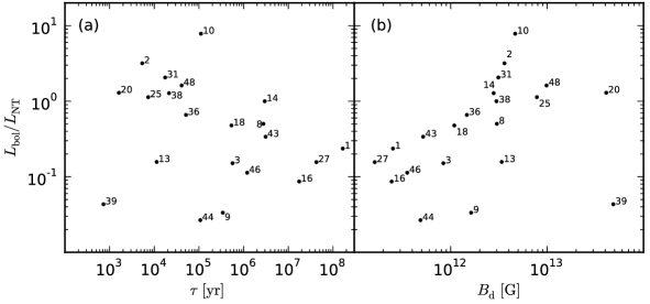
Figure 1.1: Ratio of X-ray luminosities (thermal and nonthermal components) as a function of $\tau$ (panel a) and $B_{{\rm d}}$ (panel b). The plots contain only those pulsars for which the BB+PL (Black-Body plus Power-Law) spectral fit exists. The number labels at the points correspond to the pulsar numbers in Table 1.1.

As it follows from the left panel of Figure 1.1, there is no obvious relation between pulsar age and the ratio of luminosities. The spectra of pulsars with a similar age may be dominated either by nonthermal (e.g. PSR B1951+32, PSR B1046-58) or thermal (e.g. PSR B0656+14, PSR J0538+2817) components. It is difficult to provide a more detailed analysis because, on the one hand, the observational errors are large and, on the other hand, a separation of thermal and nonthermal components is often not possible. The ratio of luminosities also does not show any correlation with the strength of the dipolar magnetic field (see the right panel of Figure 1.1). Let us note that the value of the dipolar magnetic field is conventionally calculated by adopting that the spin-down luminosity is equal to the power of magneto-dipole radiation (neglecting the influence of a pulsar wind). Then, assuming a dipolar structure of the neutron star magnetic field down to the stellar surface, we estimate its strength (measured in Gauss) at the pole as

$$B_{{\rm d}}=2.02\times 10^{12}\left(P\dot{P}_{-15}\right)^{0.5}.$$ (1.1)

Here $P$ is a period in seconds and $\dot{P}_{-15}=\dot{P}\times 10^{15}$. The actual strength of the surface magnetic field can greatly exceed the above value (see Chapter 2).

Table 1.1 presents the basic parameters of the 48 pulsars that we use in this thesis, while the results of the X-ray observations of these pulsars are listed in Tables 1.2 and 1.4.

Table 1.1: Parameters of rotation powered normal pulsars with detected X-ray radiation. The individual columns are as follows: (1) Pulsar name, (2) Barycentric period $P$ of the pulsar, (3) Time derivative of barycentric period $\dot{P}$, (4) Canonical value of the dipolar magnetic field $B_{{\rm d}}$ at the poles, (5) Spin-down energy loss rate $L_{{\rm SD}}$ (spin-down luminosity) , (6) Dispersion measure $DM$, (7) Best estimate of pulsar distance $D$ (used in all calculations), (8) Best estimate of pulsar age or spin-down age $\tau=P/\left(2\dot{P}\right)$, (9) Pulsar number (used in the Figures). Parameters of the radio pulsar have been taken from the ATNF catalogue.

Name	$P$	$\dot{P}$	$B_{{\rm d}}$	$\log L_{{\rm SD}}$	$DM$	$D$	$\tau$	No.
	$\left({\rm s}\right)$	$\left(10^{-15}\right)$	$\left(10^{12}\,{\rm G}\right)$	$\left({\rm erg\,s^{-1}}\right)$	$\left({\rm cm^{-3}\,pc}\right)$	$\left({\rm kpc}\right)$
J0108–1431	$0.808$	$0.077$	$0.504$	$30.76$	$2.38$	$0.18$	$166$ Myr	1
J0205+6449	$0.066$	$193.9$	$7.210$	$37.43$	$141$	$3.20$	$5.37$ kyr	2
B0355+54	$0.156$	$4.397$	$1.675$	$34.65$	$57.1$	$1.04$	$564$ kyr	3
B0531+21	$0.033$	$422.8$	$7.555$	$38.66$	$56.8$	$2.00$	$1.24$ kyr	4
J0537–6910	$0.016$	$51.78$	$1.846$	$38.69$	–	$47.0$	$4.93$ kyr	5
J0538+2817	$0.143$	$3.669$	$1.464$	$34.69$	$39.6$	$1.20$	$30.0$ kyr	6
B0540–69	$0.050$	$478.9$	$9.934$	$38.18$	$146$	$55.0$	$1.67$ kyr	7
B0628–28	$1.244$	$7.123$	$6.014$	$32.18$	$34.5$	$1.45$	$2.77$ Myr	8
J0633+1746	$0.237$	$10.97$	$3.258$	$34.51$	–	$0.16$	$342$ kyr	9
B0656+14	$0.385$	$55.00$	$9.294$	$34.58$	$14.0$	$0.29$	$111$ kyr	10
J0821–4300	$0.113$	$1.200$	$0.743$	$34.52$	–	$2.20$	$3.7$ kyr	11
B0823+26	$0.531$	$1.709$	$1.924$	$32.65$	$19.5$	$0.34$	$4.92$ Myr	12
B0833–45	$0.089$	$125.0$	$6.750$	$36.84$	$68.0$	$0.21$	$11.3$ kyr	13
B0834+06	$1.274$	$6.799$	$5.945$	$32.11$	$12.9$	$0.64$	$2.97$ Myr	14
B0943+10	$1.098$	$3.493$	$3.956$	$32.00$	$15.4$	$0.63$	$4.98$ Myr	15
B0950+08	$0.253$	$0.230$	$0.487$	$32.75$	$2.96$	$0.26$	$17.5$ Myr	16
B1046–58	$0.124$	$96.32$	$6.972$	$36.30$	$129$	$2.70$	$20.3$ kyr	17
B1055–52	$0.197$	$5.833$	$2.166$	$34.48$	$30.1$	$0.75$	$535$ kyr	18
J1105–6107	$0.063$	$15.83$	$2.020$	$36.40$	$271$	$7.00$	$63.3$ kyr	19
J1119–6127	$0.408$	$4022$	$81.80$	$36.36$	$707$	$8.40$	$1.61$ kyr	20
Continued on next page

Table 1.1 - continued from previous page Name $P$ $\dot{P}$ $B_{{\rm d}}$ $\log L_{{\rm SD}}$ $DM$ $D$ $\tau$ No. $\left({\rm s}\right)$ $\left(10^{-15}\right)$ $\left(10^{12}\,{\rm G}\right)$ $\left({\rm erg\,s^{-1}}\right)$ $\left({\rm cm^{-3}\,pc}\right)$ $\left({\rm kpc}\right)$ J1124–5916 $0.135$ $747.1$ $20.31$ $37.08$ $330$ $6.00$ $2.87$ kyr 21 B1133+16 $1.188$ $3.734$ $4.254$ $31.94$ $4.86$ $0.36$ $5.04$ Myr 22 J1210–5226 $0.424$ $0.066$ $0.338$ $31.53$ – $2.45$ $102$ Myr 23 B1259–63 $0.048$ $2.276$ $0.666$ $35.91$ $147$ $2.00$ $332$ kyr 24 J1357–6429 $0.166$ $360.2$ $15.62$ $36.49$ $128$ $2.50$ $7.31$ kyr 25 J1420–6048 $0.068$ $83.17$ $4.810$ $37.00$ $360$ $8.00$ $13.0$ kyr 26 B1451–68 $0.263$ $0.098$ $0.325$ $32.32$ $8.60$ $0.48$ $42.5$ Myr 27 J1509–5850 $0.089$ $9.170$ $1.824$ $35.71$ $138$ $2.56$ $154$ kyr 28 B1509–58 $0.151$ $1537$ $30.73$ $37.26$ $252$ $4.18$ $1.55$ kyr 29 J1617–5055 $0.069$ $135.1$ $6.183$ $37.20$ $467$ $6.50$ $8.13$ kyr 30 B1706–44 $0.102$ $92.98$ $6.235$ $36.53$ $75.7$ $2.50$ $17.5$ kyr 31 B1719–37 $0.236$ $10.85$ $3.234$ $34.52$ $99.5$ $1.84$ $345$ kyr 32 J1747–2958 $0.099$ $61.32$ $4.972$ $36.40$ $102$ $5.00$ $25.5$ kyr 33 B1757–24 $0.125$ $127.9$ $8.075$ $36.41$ $289$ $5.00$ $15.5$ kyr 34 B1800–21 $0.134$ $134.1$ $8.551$ $36.34$ $234$ $4.00$ $15.8$ kyr 35 J1809–1917 $0.083$ $25.54$ $2.936$ $36.26$ $197$ $3.50$ $51.3$ kyr 36 J1811–1925 $0.065$ $44.00$ $3.407$ $36.81$ – $5.00$ $23.3$ kyr 37 B1823–13 $0.101$ $75.06$ $5.575$ $36.45$ $231$ $4.00$ $21.4$ kyr 38 J1846–0258 $0.326$ $7083$ $97.02$ $36.91$ – $6.00$ $0.73$ kyr 39 B1853+01 $0.267$ $208.4$ $15.08$ $35.63$ $96.7$ $2.60$ $20.3$ kyr 40 B1916+14 $1.181$ $212.4$ $31.99$ $33.71$ $27.2$ $2.10$ $88.1$ kyr 41 J1930+1852 $0.137$ $750.6$ $20.47$ $37.08$ $308$ $5.00$ $2.89$ kyr 42 B1929+10 $0.227$ $1.157$ $1.034$ $33.59$ $3.18$ $0.36$ $3.10$ Myr 43 B1951+32 $0.040$ $5.845$ $0.971$ $36.57$ $45.0$ $2.00$ $107$ kyr 44 J2021+3651 $0.104$ $95.60$ $6.361$ $36.53$ $371$ $10.0$ $17.2$ kyr 45 J2043+2740 $0.096$ $1.270$ $0.706$ $34.75$ $21.0$ $1.80$ $1.20$ Myr 46 B2224+65 $0.683$ $9.659$ $5.187$ $33.08$ $36.1$ $2.00$ $1.12$ Myr 47 B2334+61 $0.495$ $191.7$ $19.69$ $34.79$ $58.4$ $3.10$ $40.9$ kyr 48

1.3 Nonthermal X-ray radiation

The nonthermal emission, which is generally observed from radio to $\gamma$-ray frequencies, should be generated by charged particles accelerated at the expense of rotational energy in the magnetosphere of the neutron star. Nonthermal X-ray radiation is characterised by highly anisotropic emission patterns, which give rise to large pulsed fractions. The pulse profiles often show narrow (often double) peaks, however, in many cases nearly sinusoidal profiles are observed. As the X-ray efficiency is strongly correlated with $L_{{\rm SD}}$, the most X-ray luminous sources (among rotationally powered pulsars) are the Crab pulsar and two young pulsars in the Large Magellanic Cloud, which are the only pulsars with $L_{{\rm SD}}>10^{38}\,{\rm erg\,s^{-1}}$ (Mereghetti,, 2011).

Becker and Truemper, (1997) suggested that in the $0.1\text{\textendash}2.4\,{\rm keV}$ band ROSAT sources that are identified as rotation-powered pulsars exhibit an X-ray efficiency which can be approximated as a linear function $L_{{\rm X}}=\xi L_{{\rm SD}}$, where the total X-ray efficiency $\xi=\xi_{{}_{{\rm BB}}}+\xi_{{}_{{\rm NT}}}\approx 10^{-3}$, here $\xi_{{}_{{\rm BB}}}$ and $\xi_{{}_{{\rm NT}}}$ are efficiencies of the thermal (without the cooling component) and nonthermal X-ray emission, respectively. The higher sensitivity of both the Chandra and XMM-Newton allows detection of less efficient ($\xi<10^{-3}$) X-ray pulsars (see Figure 1.2). Becker, (2009) suggested that for these faint pulsars the orientation of the magnetic/rotation axes to the observer’s line of sight might not be optimal. We believe that the efficiency of spin-down energy conversion processes is mostly affected by the strength and structure of the surface magnetic field. The variation of $\xi$ is rather due to the nature of physical processes than the geometrical effects. Let us note that the nonthermal X-ray luminosities presented in Figure 1.2 are calculated assuming an isotropic radiation pattern. In general, the X-ray emission pattern differs quite essentially from the isotropic one. Thus, one should introduce a beaming factor as the ratio of the opening angle of the radiation cone to the full solid angle $4\pi$. Since a beaming factor is generally unknown, the actual X-ray efficiency may differ by up to an order of magnitude (or even more) than we have presented.

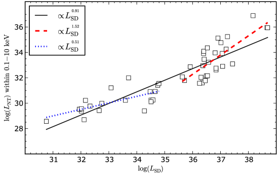
Figure 1.2: Nonthermal luminosity within the $0.1-10\,{\rm keV}$ band ($L_{{\rm NT}}$) vs spin-down luminosity ($L_{{\rm SD}}$). The black solid line corresponds to the linear fitting for all pulsars, while the blue dotted and red dashed lines correspond to the linear fit for less luminous ($L_{{\rm SD}}<10^{35}\,{\rm erg\,s^{-1}}$) and more luminous ($L_{{\rm SD}}>10^{35}\,{\rm erg\,s^{-1}}$) pulsars, respectively.

Various fitting parameters and efficiencies of nonthermal X-ray radiation suggest that the efficiency of processes responsible for the generation of nonthermal X-ray radiation should highly depend on the pulsar parameters (see Figure 1.2). The fitting parameters for the data of all pulsars show a linear trend with $\xi\approx 10^{-3}$, however, if we divide them into two groups of less and more luminous pulsars, we can see that the fitting parameters for these two groups differ from one another. The efficiency of less luminous X-ray pulsars depends on $L_{{\rm SD}}$ to a lesser extent than is the case for more luminous pulsars.

As we mentioned in the Introduction, there are two main types of models: the polar cap models and the outer gap models. The outer gap model was proposed to explain the bright $\gamma$-ray emission from the Crab and Vela pulsars (Cheng et al., 1986a, ; Cheng et al., 1986b, ). Placing a $\gamma$-ray emission zone at the light cylinder, where the magnetic field strength is considerably reduced to $B_{{\rm LC}}=B_{{\rm d}}\left(R/R_{{\rm LC}}\right)^{3}$, provides higher $\gamma$-ray emissivities that are in somewhat better agreement with the observations. The observational data can be interpreted with any of the two models, although under completely different assumptions about pulsar parameters.

1.3.1 Observations

Generally, the X-ray spectrum of relatively young ($\tau<10\,{\rm kyr}$) and middle-aged ($\tau<10\,{\rm kyr}$) pulsars is dominated by the nonthermal component. However, it is not possible to find an exact correlation between $\tau$ and the type of spectra, i.e. which component, thermal or nonthermal, dominates the spectrum (see the left panel of Figure 1.1). As we mentioned above, it is quite often impossible to resolve the components. The Crab pulsar ($\tau=958\,{\rm yrs}$) is the most characteristic example of a young pulsar. The upper limit for X-ray luminosity of the Crab pulsar (one of the strongest known X-ray radio pulsars) is about $L_{{\rm NT}}^{{\rm{}^{max}}}=8.9\times 10^{35}\,{\rm erg\,s^{-1}}$. This value is calculated assuming an isotropic radiation pattern, however, even if we assume an angular anisotropy of the radiation (beaming factor $\approx 1/4\pi$), the lower limit of its luminosity $L_{{\rm NT}}^{{}^{{\rm min}}}=7.1\times 10^{34}\,{\rm erg\,s^{-1}}$ continues to be very high. The luminosities calculated above correspond to the following X-ray efficiencies: ${\displaystyle\xi_{{}_{{\rm NT}}}^{{}^{{\rm max}}}=10^{-2.71}}$ (isotropic radiation pattern) and $\xi_{{}_{{\rm NT}}}^{{\rm{}^{min}}}=10^{-3.81}$ (anisotropic radiation pattern). Although ${\displaystyle\xi_{{}_{{\rm NT}}}}$ is quite small, the nonthermal component still obscures all the thermal ones. To obtain a similar efficiency of the thermal radiation from the entire stellar surface, its temperature should be $T_{{\rm s}}=5.9\times 10^{6}\,{\rm K}$ (assuming $R=10\,{\rm km}$), which vastly exceeds the upper limit ($T_{{\rm s}}<2.3\times 10^{6}\,{\rm K}$). Furthermore, the temperature of the polar caps should be about $2.5\times 10^{7}\,{\rm K}$ to obtain a comparable luminosity.

The Vela-like pulsars compose another characteristic group of pulsars. This group consists of pulsars with high spin-down luminosities but considerably low X-ray efficiencies $\xi_{{}_{{\rm NT}}}\apprle 10^{-4}$. A characteristic age of the Vela is about $1.1\times 10^{4}\,{\rm yrs}$ ($10$ times older than the Crab), but it can still be classified as a very young pulsar. The nonthermal luminosity of a Vela pulsar is $L_{{\rm NT}}^{{}^{{\rm max}}}=4.2\times 10^{32}$ and efficiency $\xi_{{}_{{\rm NT}}}^{{}^{{\rm max}}}=10^{-4.22}$. Some of the Vela-like pulsars (like the Vela itself) also exhibit a thermal component, which in some cases can be comparable to the nonthermal component. The thermal efficiency of the Vela $\xi_{{}_{{\rm BB}}}=10^{-4.72}$ is quite similar to $\xi_{{}_{{\rm NT}}}^{{}^{{\rm max}}}=10^{-4.22}$, but if we assume an anisotropic radiation pattern of the nonthermal component than $\xi_{{}_{{\rm NT}}}^{{}^{{\rm min}}}=10^{-5.32}$, thus even less than $\xi_{{}_{{\rm BB}}}$.

The third group includes pulsars with low spin-down luminosity $L_{{\rm SD}}\apprle 10^{35}$. In most cases, the X-ray spectra of such pulsars (e.g. PSR 9050+08, PSR B1929+10) have both thermal and nonthermal components, with similar efficiencies. Thus, the spectrum fitting procedure is more complicated. The nonthermal X-ray efficiencies of these pulsars, $\xi_{{}_{{\rm NT}}}\sim 10^{-3}$, are considerably higher than those of the Vela-like pulsars. Note that even when the observed spectra are dominated by nonthermal radiation, we cannot rule out a situation that the thermal component is stronger than the nonthermal one, but due to unfavourable geometry we cannot observe it.

Even with the improved quality of X-ray observations performed by both the Chandra and XMM-Newton, the available data do not allow us to fully discriminate between the different emission scenarios. However, these data can be used to verify whether the proposed model of X-ray emission meets all the requirements. Table 1.2 presents the observed spectral properties of pulsars showing nonthermal components.

Table 1.2: Observed spectral properties of rotation-powered pulsars with X-ray spectrum showing the nonthermal (power-law) component. The individual columns are as follows: (1) Pulsar name, (2) Additional information, (3) Spectral components required to fit the observed spectra, PL: power law, BB: blackbody, (4) Pulse phase average photon index, (5) Maximum nonthermal luminosity $L_{{\rm NT}}$, (6) Maximum nonthermal X-ray efficiency $\xi_{{}_{{\rm NT}}}^{{}^{{\rm max}}}$, (7) Minimum nonthermal X-ray efficiency $\xi_{{}_{{\rm NT}}}^{{\rm{}^{min}}}$, (8) Total thermal luminosity $L_{{\rm BB}}$, (9) Thermal efficiency $\xi_{{}_{{\rm BB}}}$, (10) References, (11) Number of the pulsar. Both nonthermal luminosities and efficiencies were calculated in the $0.1-10\,{\rm keV}$ band. The maximum value was calculated with the assumption that the X-ray radiation is isotropic while the minimum value was calculated assuming strong angular anisotropy of the radiation ($\xi_{{}_{{\rm NT}}}^{{\rm{}^{min}}}\approx 1/\left(4\pi\right)\cdot\xi_{{}_{{\rm NT}}}^{{\rm{}^{max}}}$). Pulsars are sorted by nonthermal X-ray luminosity (5).

Name	Comment	Spectrum	Photon-Index	$\log L_{{\rm NT}}$	$\log\xi_{{}_{{\rm NT}}}^{{\rm{}^{max}}}$	$\log\xi_{{}_{{\rm NT}}}^{{}^{{\rm min}}}$	$\log L_{{\rm BB}}$	$\log\xi_{{}_{{\rm BB}}}$	Ref.	No.
				$\left({\rm erg\,s^{-1}}\right)$			$\left({\rm erg\,s^{-1}}\right)$
B0540–69	N158A, LMC	PL	$1.92_{-0.11}^{+0.11}$	$36.90$	$-1.27$	$-2.37$	–	–	Ka01, Ca08	7
B0531+21	Crab	PL	$1.63_{-0.07}^{+0.07}$	$35.95$	$-2.71$	$-3.81$	–	–	Be09	4
J0537–6910	N157B, LMC	PL	$1.80_{-0.10}^{+0.10}$	$35.95$	$-2.74$	$-3.84$	–	–	Mi05	5
B1509–58	Crab-like pulsar	PL	$1.19_{-0.04}^{+0.04}$	$35.24$	$-2.00$	$-3.10$	–	–	Cu01, De06, Be09	29
J1846–0258	Kes 75	BB + PL	$1.90_{-0.10}^{+0.10}$	$35.13$	$-1.78$	$-2.88$	$34.06$	$-2.85$	Ng08, He03	39
J1420–6048		PL	$1.60_{-0.40}^{+0.40}$	$34.77$	$-2.25$	$-3.35$	–	–	Ro01	26
J2021+3651		PL, BB	$1.70_{-0.20}^{+0.30}$	$34.36$	$-2.17$	$-3.27$	$33.78$	$-2.75$	Va08,He04	45
J1617–5055	Crab-like pulsar	PL	$1.14_{-0.06}^{+0.06}$	$34.25$	$-2.95$	$-4.05$	–	–	Ka09, Be02	30
J1747–2958	Mouse	PL, BB	$1.80_{-0.08}^{+0.08}$	$34.09$	$-2.31$	$-3.41$	–	–	Ga04	33
J1811–1925	G11.2-0.3	PL	$0.97_{-0.32}^{+0.39}$	$33.97$	$-2.84$	$-3.94$	–	–	Ro03, Ro04	37
J1930+1852	Crab-like pulsar	PL	$1.20_{-0.20}^{+0.20}$	$33.92$	$-3.15$	$-4.25$	–	–	Lu07, Ca02	42
Continued on next page

Table 1.2 - continued from previous page Name Comment Spectrum Photon-Index $\log L_{{\rm NT}}$ $\log\xi_{{}_{{\rm NT}}}^{{}^{max}}$ $\log\xi_{{}_{{\rm NT}}}^{{}^{min}}$ $\log L_{{\rm BB}}$ $\log\xi_{{}_{{\rm BB}}}$ Ref. No. $\left({\rm erg\,s^{-1}}\right)$ $\left({\rm erg\,s^{-1}}\right)$ J1105–6107 PL $1.80_{-0.40}^{+0.40}$ $33.91$ $-2.48$ $-3.58$ – – Go98 19 B1757–24 Duck PL $1.60_{-0.50}^{+0.60}$ $33.46$ $-2.95$ $-4.05$ – – Ka01 34 B1951+32 CTB 80 BB + PL $1.63_{-0.05}^{+0.03}$ $33.22$ $-3.35$ $-4.45$ $31.95$ $-4.62$ Li05 44 J0205+6449 3C58 BB + PL $1.78_{-0.04}^{+0.02}$ $33.10$ $-4.33$ $-5.43$ $33.60$ $-3.83$ Sl04 2 J1119–6127 G292.2-0.5 BB + PL $1.50_{-0.20}^{+0.30}$ $32.95$ $-3.42$ $-4.51$ $33.37$ $-3.00$ Go07, Ng12 20 J1124–5916 Vela-like pulsar PL $1.60_{-0.10}^{+0.10}$ $32.91$ $-4.17$ $-5.27$ – – Hu03,Go03 21 B1259–63 Be-star bin PL $1.69_{-0.04}^{+0.04}$ $32.87$ $-3.05$ $-4.15$ – – Ch09, Ch06 24 B0833–45 Vela BB + PL $2.70_{-0.40}^{+0.40}$ $32.62$ $-4.22$ $-5.32$ $32.12$ $-4.72$ Za07b 13 B1706–44 G343.1-02.3 BB + PL $2.00_{-0.50}^{+0.50}$ $32.16$ $-4.37$ $-5.47$ $32.78$ $-3.76$ Go02 31 J1357–6429 BB + PL $1.30_{-0.20}^{+0.20}$ $32.15$ $-4.35$ $-5.44$ $32.50$ $-3.99$ Za07 25 B1853+01 W44 PL $1.28_{-0.48}^{+0.48}$ $32.07$ $-3.57$ $-4.66$ – – Pe02 40 B1046–58 Vela-like pulsar PL $1.70_{-0.20}^{+0.40}$ $32.04$ $-4.26$ $-5.36$ – – Go06 17 B1916+14 BB, PL $3.50_{-0.70}^{+1.60}$ $32.00$ $-1.71$ $-2.81$ $31.07$ $-2.63$ Zh09 41 J1509–5850 MSH 15-52 PL $1.00_{-0.30}^{+0.20}$ $31.80$ $-3.92$ $-5.02$ – – Hu07 28 B1823–13 Vela-like BB + PL $1.70_{-0.70}^{+0.70}$ $31.78$ $-4.67$ $-5.77$ $32.19$ $-4.27$ Pa08 38 B1800–21 Vela-like pulsar PL + BB $1.40_{-0.60}^{+0.60}$ $31.60$ $-4.74$ $-5.84$ – – Ka07 35 Continued on next page

Table 1.2 - continued from previous page Name Comment Spectrum Photon-Index $\log L_{{\rm NT}}$ $\log\xi_{{}_{{\rm NT}}}^{{}^{max}}$ $\log\xi_{{}_{{\rm NT}}}^{{}^{min}}$ $\log L_{{\rm BB}}$ $\log\xi_{{}_{{\rm BB}}}$ Ref. No. $\left({\rm erg\,s^{-1}}\right)$ $\left({\rm erg\,s^{-1}}\right)$ J1809–1917 BB + PL $1.23_{-0.62}^{+0.62}$ $31.57$ $-4.68$ $-5.78$ $31.69$ $-4.56$ Ka07 36 B2334+61 BB + PL $2.20_{-1.40}^{+3.00}$ $31.55$ $-3.24$ $-4.34$ $32.06$ $-2.73$ Mc06 48 J2043+2740 BB + PL $2.80_{-0.80}^{+1.00}$ $31.41$ $-3.34$ $-4.44$ $30.77$ $-3.98$ Be04 46 B2224+65 Guitar PL, BB $2.20_{-0.30}^{+0.20}$ $31.21$ $-1.87$ $-2.97$ $30.51$ $-2.57$ Hu12, Hu07b 47 B0355+54 BB + PL $1.00_{-0.20}^{+0.20}$ $30.92$ $-3.73$ $-4.83$ $30.40$ $-4.25$ Mc07,Sl94 3 B1055–52 BB+BB+PL $1.70_{-0.10}^{+0.10}$ $30.91$ $-3.57$ $-4.67$ $32.63$ $-1.85$ De05 18 B0656+14 BB+BB+PL $2.10_{-0.30}^{+0.30}$ $30.26$ $-4.33$ $-5.42$ $32.77$ $-1.81$ De05 10 J0633+1746 Geminga BB+BB+PL $1.68_{-0.06}^{+0.06}$ $30.24$ $-4.27$ $-5.37$ $31.67$ $-2.84$ Ja05 9 B1929+10 BB + PL $1.73_{-0.66}^{+0.46}$ $30.23$ $-3.36$ $-4.46$ $30.06$ $-3.53$ Mi08 43 B0628–28 BB + PL $2.98_{-0.65}^{+0.91}$ $30.22$ $-1.94$ $-3.04$ $30.22$ $-1.94$ Te05 , Be05 8 B0950+08 BB + PL $1.31_{-0.14}^{+0.14}$ $29.99$ $-2.76$ $-3.86$ $28.92$ $-3.82$ Za04 16 B1451–68 BB + PL $1.40_{-0.50}^{+0.50}$ $29.77$ $-2.56$ $-3.66$ $29.27$ $-3.06$ Po12 27 B1133+16 BB, PL $2.51_{-0.33}^{+0.36}$ $29.52$ $-2.42$ $-3.52$ $28.56$ $-3.38$ Ka06 22 B0823+26 PL $1.58_{-0.33}^{+0.43}$ $29.42$ $-3.23$ $-4.33$ – – Be04 12 B0943+10 Chameleon BB, PL $2.60_{-0.50}^{+0.70}$ $29.38$ $-2.64$ $-3.74$ $28.40$ $-3.62$ Zh05,Ka06 15 B0834+06 BB + PL – $28.70$ $-3.41$ $-4.51$ $28.70$ $-3.41$ Gi08 14 J0108–1431 BB + PL $3.10_{-0.20}^{+0.50}$ $28.57$ $-2.19$ $-3.29$ $27.94$ $-2.82$ Po12, Pa09 1

1.4 Thermal X-ray radiation

1.4.1 Modelling of thermal radiation from a neutron star

Thermal X-ray emission seems to be quite a common feature of radio pulsars. The blackbody fit to the observed thermal spectrum of a neutron star allows us to obtain the redshifted effective temperature $T^{\infty}$ and redshifted total bolometric flux $F^{\infty}$ (measured by a distant observer). To estimate the actual (unredshifted) parameters, one should take into account the gravitational redshift, $g_{{\rm r}}=\sqrt{1-2GM/Rc^{2}}$, determined by the neutron star mass $M$ and radius $R$, here $G$ is the gravitational constant. Then the actual effective temperature and actual total bolometric flux can be written as:

$$\begin{split}T&=g_{{\rm r}}^{-1}T^{\infty},\\ F&=g_{{\rm r}}^{-2}F^{\infty}.\end{split}$$ (1.2)

Knowing the distance to the neutron star, $D$, we can use the effective temperature and total bolometric flux to calculate the size of the radiating region. If we assume that the radiation is isotropic (same in all directions, e.g. radiation from the entire stellar surface) then the radius of the radiating sphere (star) can be calculated as (Zavlin, 2007a, )

$$R_{\perp}^{\infty}=D\sqrt{\frac{F^{\infty}}{\sigma T^{\infty 4}}}=g_{{\rm r}}^{-1}R_{\perp},$$ (1.3)

where $\sigma\approx 5.6704\times 10^{-5}{\rm\,erg\,cm^{-2}\,s^{-1}\,K^{-4}}$ is the Stefan-Boltzmann constant.

Knowing that $L_{{\rm BB}}=4\pi D^{2}F$ and using Equations 1.2 and 1.3, we can write that

$$L_{{\rm BB}}=g_{{\rm r}}^{-2}L_{{\rm BB}}^{\infty}.$$ (1.4)

The modelling of thermal radiation is more complicated if we assume that it comes from the hot spot on the stellar surface. One should take into account such factors as: time-averaged cosine of the angle between the magnetic axis and the line of sight $\left<\cos i\right>$, gravitational bending of light, as well as whether the radiation comes from two opposite poles of the star or from one hot spot only. In general, the observed luminosity of the hot spot can be written as:

$$L_{{\rm hs}}^{\infty}=A_{{\rm hs}}^{\infty}\sigma T^{\infty 4},$$ (1.5)

where $A_{{\rm hs}}^{\infty}=\pi R_{{\rm hs}}^{\infty 2}$ is the observed area of the radiating region.

The observed area of the radiating spot is also influenced by the geometrical factor $f$. This geometrical factor depends on following angles: $\zeta$ between the line of sight and the spin axis, and $\alpha$ between the spin and magnetic axes, as well as on $g_{{\rm r}}$ and whether the radiation comes from the star’s two opposite poles or from a single hot spot only:

$$\begin{split}A_{{\rm hs}}^{\infty}&=g_{{\rm r}}^{-2}fA_{{\rm hs}},\\ R_{{\rm hs}}&=g_{{\rm r}}f^{-1/2}R_{{\rm hs}}^{\infty}.\end{split}$$ (1.6)

Finally, the hot spot luminosity can be calculated as

$$L_{{\rm hs}}=g_{{\rm r}}^{-2}f^{-1}L_{{\rm hs}}^{\infty}.$$ (1.7)

The luminosity of a radiating sphere with radius $R_{\perp}$ can be calculated as $L_{{\rm sp}}=4A_{\perp}\sigma T^{4}=4\pi R_{\perp}^{2}\sigma T^{4}$. On the other hand, if we assume that the radiation originates only from one hot spot we can calculate the luminosity as $L_{{\rm hs}}=A_{{\rm hs}}\sigma T^{4}$. If the hot spot size is small compared to the star radius ($R_{{\rm hs}}\ll R$) then the area of the spot can be calculated as $A_{{\rm hs}}\approx\pi R_{\perp}^{2}$. Thus, we have to remember that the luminosity calculated assuming a spherical source will be four times higher than the actual luminosity of a radiating hot spot $L_{{\rm hs}}=1/4\cdot L_{{\rm sp}}$ (see the next section for details).

1.4.2 Thermal radiation of hot spots

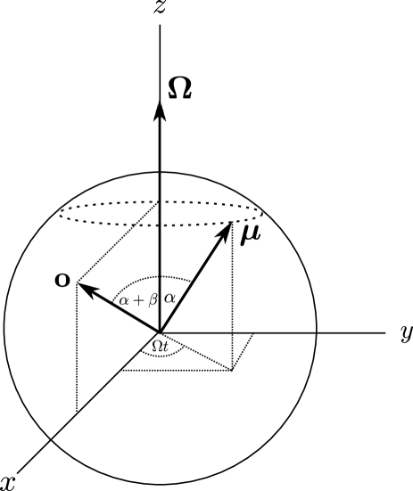
Figure 1.3: Coordinate system co-rotating with a star. The system was chosen so that the z-axis is along ${\bf\Omega}$ (the angular velocity) and ${\bf o}$ lies in the x-z plane (fiducial plane, i.e. at longitude zero). Here, $\boldsymbol{\hat{\mu}}$ is a unit vector in the direction of the magnetic axis and $\alpha$ is the angle between ${\bf\Omega}$ and $\boldsymbol{\hat{\mu}}$, $\beta$ is the impact parameter.

Let us consider a neutron star with two antipodal hot spots associated with polar caps of a stellar magnetic field. For simplicity’s sake we assume that the spot size is small compared to the star radius $R$. If the magnetic axis $\boldsymbol{\hat{\mu}}$ is inclined to the spin axis by an angle $\alpha\leq 90^{\circ}$, the spots periodically change their position and inclination with respect to a distant observer. To compute the radiation fluxes from the primary (closer to the observer) as well as the antipodal spot, we need to know their inclinations: $\cos i_{1}={\bf n\cdot o}$ and $\cos i_{2}={\bf\bar{n}\cdot o}=-\cos i_{1}$, where ${\bf n}$ and ${\bf\bar{n}}=-{\bf n}$ are normal vectors to spots surfaces, and ${\bf o}$ is the unit vector pointing toward the observer. In the calculations we use a coordinate system co-rotating with a star. The z-axis is along ${\bf\Omega}$ (the angular velocity) and ${\bf o}$ lies in the x-z plane (see Figure 1.3).

In the chosen coordinate system we can write that the spherical coordinates of vectors have the following components:

$$\begin{array}[]{ccc}{\bf\Omega}&=&\left(\Omega,\,0,\,0\right);\\ {\bf o}&=&\left(1,\,\alpha+\beta,\,0\right);\\ \boldsymbol{\hat{\mu}}&=&\left(1,\,\alpha,\,\Omega t\right).\end{array}$$ (1.8)

Here the impact parameter $\beta$ represents the closest approach of the line of sight to the magnetic axis. Note that $\boldsymbol{\hat{\mu}}={\bf n}$ and ${\bf\bar{{\bf n}}}=-\boldsymbol{\hat{\mu}}$; thus, we can write the following components of Cartesian coordinates:

$$\begin{array}[]{ccc}{\bf{\bf o}}&=&\left(\sin\left(\alpha+\beta\right),\,0,\,\cos\left(\alpha+\beta\right)\right);\\ {\bf n}&=&\left(\sin\alpha\cos\Omega t,\,\sin\Omega t\sin\alpha,\,\cos\alpha\right).\end{array}$$ (1.9)

Finally, the inclination angle for both primary and antipodal hot spots can be calculated as

$$\begin{array}[]{ccc}\cos i_{1}&=&\sin\alpha\cdot\cos\Omega t\cdot\sin\left(\alpha+\beta\right)+\cos\alpha\cdot\cos\left(\alpha+\beta\right);\\ \cos i_{2}&=&-\cos i_{1}=-\sin\alpha\cdot\cos\Omega t\cdot\sin\left(\alpha+\beta\right)-\cos\alpha\cdot\cos\left(\alpha+\beta\right).\end{array}$$ (1.10)

We can estimate the contributions of the primary and antipodal spots to the observed X-ray flux by calculating the time-averaged cosine of the angle between the magnetic axis and the line of sight. Note that we should take into account only positive values of $\cos i$ since for larger angles ($i>90^{\circ}$) the spot is not visible (at least in this approximation, see Section 1.4.3 for more details). Thus, the contribution of the primary spot can be calculated as follows:

$$\begin{array}[]{c}\left\langle\cos i_{1}\right\rangle=\begin{cases}\begin{split}\int_{0}^{P}\cos\left(i_{1}\right){\rm d}t\end{split}&{\rm if}\ \frac{1}{\tan\alpha\tan\left(\alpha+\beta\right)}<-1\ {\rm or}\ \frac{1}{\tan\alpha\tan\left(\alpha+\beta\right)}>1,\\ \begin{split}\int_{0}^{t_{-}}\cos\left(i_{1}\right){\rm d}t\end{split}+\begin{split}\int_{t_{+}}^{2\pi}\cos\left(i_{1}\right){\rm d}t\end{split}&{\rm if}\ -1<\frac{1}{\tan\alpha\tan\left(\alpha+\beta\right)}<1,\end{cases}\end{array}$$ (1.11)

where integration limits are

$$t_{\pm}=\frac{P}{2}\pm\frac{P}{2\pi}\arccos\left[\frac{1}{\tan\alpha\tan\left(\alpha+\beta\right)}\right].$$ (1.12)

On the other hand, the contribution of the antipodal spot can be calculated as

$$\begin{array}[]{c}\left\langle\cos i_{2}\right\rangle=\begin{cases}\begin{split}0\end{split}&{\rm if}\ \frac{1}{\tan\alpha\tan\left(\alpha+\beta\right)}<-1\ {\rm or}\ \frac{1}{\tan\alpha\tan\left(\alpha+\beta\right)}>1,\\ \begin{split}\int_{t_{-}}^{t_{+}}\cos\left(i_{2}\right){\rm d}t\end{split}&{\rm if}\ -1<\frac{1}{\tan\alpha\tan\left(\alpha+\beta\right)}<1.\end{cases}\end{array}$$ (1.13)

Depending on the orientation of ${\bf\Omega}$, ${\bf o}$ and $\boldsymbol{\hat{\mu}}$, the thermal radiation may originate from: (1) both the primary and antipodal hot spots (see Figure 1.4); (2) mainly the primary spot but with a small contribution from the antipodal spot (see Figure 1.5); (3) the primary spot only (see Figure 1.6).

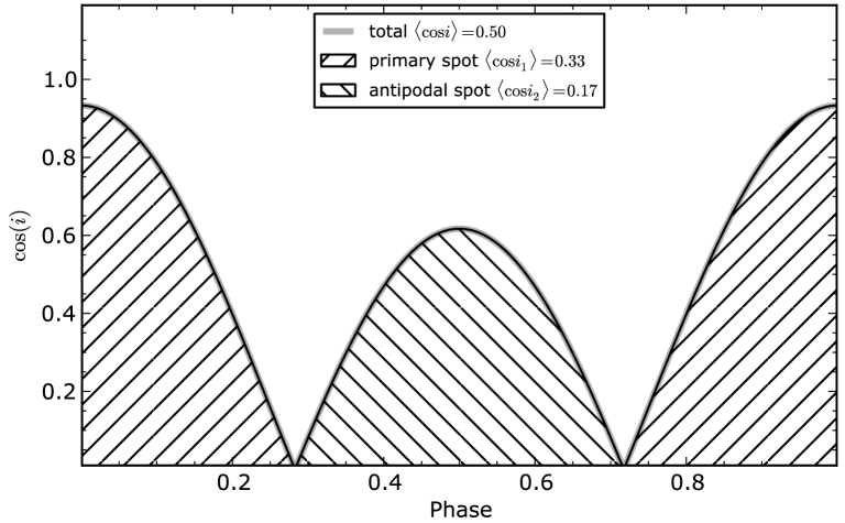
Figure 1.4: Cosine of the hot spots’ inclination angle as a function of the pulsar phase for PSR B0950+08. The following parameters were used: $\alpha=105.46^{\circ}$, $\beta=21.1^{\circ}$. For this geometry the thermal radiation of both primary and antipodal spots has a significant influence on the observed thermal flux.

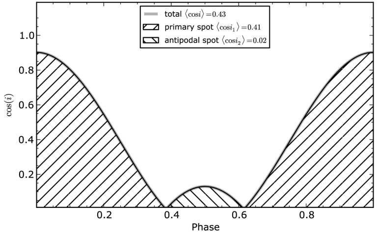
Figure 1.5: Cosine of the hot spots’ inclination angle as a function of the pulsar phase for PSR B1929+10. The following parameters were used: $\alpha=35.97$, $\beta=25.55$. For this geometry there is only a small contribution from the antipodal spot.

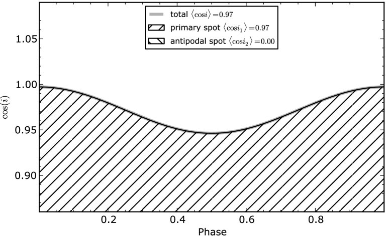
Figure 1.6: Cosine of the hot spots’ inclination angle as a function of the pulsar phase for PSR B0943+10. The following parameters were used: $\alpha=11.58^{\circ}$, $\beta=-4.29^{\circ}$. For this geometry only the primary hot spot is visible.

1.4.3 Gravitational bending of light near stellar surface

The radius of a neutron star is only a few times larger than the Schwarzschild radius. The approach presented in the previous section does not include the gravitational bending effect, which is very strong in neutron stars. A strong gravitational field just above the stellar surface causes the bending of light. A photon emitted near a neutron star surface at an angle $\delta$ with respect to the radial direction escapes to infinity at a different angle $\delta^{\prime}>\delta$. As a consequence, even when the spot inclination angle to the line of sight is $i\gtrsim 90^{\circ}$ we can still observe thermal radiation from this spot. For a Schwarzschild metric we can calculate an observed flux fraction from the primary $f_{1}=F_{1}/F_{0}$ and antipodal $f_{2}=F_{2}/F_{0}$ spots. Here $F_{0}$ is the maximum possible flux that is observed when the primary spot is viewed face-on. The primary and antipodal fluxes are given by (Beloborodov,, 2002)

$$\begin{array}[]{ccc}f_{1}&=&\cos\left(i\right)\left(1-\frac{r_{{\rm g}}}{R}\right)+\frac{r_{{\rm g}}}{R},\\ f_{2}&=&-\cos\left(i\right)\left(1-\frac{r_{{\rm g}}}{R}\right)+\frac{r_{{\rm g}}}{R},\end{array}$$ (1.14)

here $r_{{\rm g}}=2GM/c^{2}$ is the Schwarzschild radius. The primary spot is visible when $\cos i_{1}>-r_{{\rm g}}/\left(R-r_{{\rm g}}\right)$ and the antipodal spot when $\cos i_{2}>-r_{{\rm g}}/\left(R-r_{{\rm g}}\right)$. Consequently, both spots are seen when $-r_{{\rm g}}/\left(R-r_{{\rm g}}\right)<\cos i<r_{{\rm g}}/\left(R-r_{{\rm g}}\right)$, and then the observed flux fraction is

$$f_{{\rm min}}=f_{1}+f_{2}=\frac{2r_{{\rm g}}}{R}.$$ (1.15)

Hence, the blackbody pulse of primary and antipodal spots must display a plateau whenever both spots are in sight. Depending on the geometry of a pulsar we can distinguish four classes (Beloborodov,, 2002). Class I: when the antipodal spot is never seen and the primary spot is visible all the time (see the bottom right panel of Figure 1.7). For such pulsars the blackbody pulse has a perfect sinusoidal shape. Class II: when the primary spot is seen all the time and the antipodal spot is also in the visible zone for some time (see panels a, b and c of Figure 1.7). For these pulsars the sinusoidal pulse shape is interrupted by the plateau. Class III: the primary spot is not visible for a fraction of the period and during this time only the antipodal spot is seen. The primary sinusoidal profile of such pulsars is interrupted by the plateau, and the plateau is interrupted by a weaker sinusoidal subpulse from the antipodal spot. Class IV: both spots are seen at any time. The observed blackbody flux of such pulsars is constant.

The gravitational bending of light can significantly increase the visibility of a pulsar (i.e. the observed flux, compare Figures 1.4 and 1.8). For some specific geometry the gravitational effects can also drastically change primary to the antipodal flux ratio (compare Figures 1.9 and 1.5). Our calculations show that for canonical values $M=1.4\,{\rm M}_{\odot}$ and $R=10\,{\rm km}$ the gravitational effect is quite strong and the observed flux fraction is in the range of $0.85-1$, while the geometric approach results in the $0.43-1$ range (see Table 1.3).

Table 1.3: Viewing geometry of pulsars. The individual columns are as follows: (1) Pulsar name, (2) Inclination angle with respect to the rotation axis $\alpha$, (3) Opening angle $\rho$, (4) Impact parameter $\beta$, (5) Total flux correction factor (including gravitational bending of light) $\left\langle f\right\rangle$ , (6) Flux correction factor of the primary spot $\left\langle f_{1}\right\rangle$, (7) Flux correction factor of the antipodal spot $\left\langle f_{2}\right\rangle$, (8, 9, 10) Time-averaged cosine of the angle between the magnetic axis and the line of sight: $\left<\cos i\right>$ (the total value), $\left<\cos i_{1}\right>$(the primary spot), $\left<\cos i_{2}\right>$ (the antipodal spot), (10) Number of the pulsar. The gravitational bending effect was calculated using $M=1.4\,{\rm M}_{\odot}$ and $R=10\,{\rm km}$.

Name	$\alpha$	$\beta$	$\rho$	$\left\langle f\right\rangle$	$\left\langle f_{1}\right\rangle$	$\left\langle f_{2}\right\rangle$	$\left<\cos i\right>$	$\left<\cos i_{1}\right>$	$\left<\cos i_{2}\right>$	No.
	$\left({\rm deg}\right)$	$\left({\rm deg}\right)$	$\left({\rm deg}\right)$
B0628–28	$70.0$	$-12.0$	$19.6$	$0.86$	$0.52$	$0.34$	$0.52$	$0.35$	$0.17$	8
B0834+06	$60.7$	$4.5$	$7.1$	$0.86$	$0.53$	$0.32$	$0.52$	$0.36$	$0.16$	14
B0943+10	$11.6$	$-4.3$	$4.5$	$0.98$	$0.98$	$0.00$	$0.97$	$0.97$	$0.00$	15
B0950+08	$105.4$	$22.1$	$25.6$	$0.85$	$0.51$	$0.34$	$0.50$	$0.33$	$0.17$	16
B1133+16	$52.5$	$4.5$	$8.1$	$0.86$	$0.61$	$0.25$	$0.48$	$0.40$	$0.07$	22
B1451–68	$37.0$	$-6.0$	–	$0.88$	$0.81$	$0.06$	$0.68$	$0.68$	$0.00$	27
B1929+10	$36.0$	$25.6$	$26.8$	$0.85$	$0.64$	$0.21$	$0.43$	$0.41$	$0.02$	43

Figure 1.7: Comparison of the observed flux fraction for geometric effect only (blue dotted line) and for geometric effect with the inclusion of a gravitational bending of light (red solid line). Individual panels correspond to the following pulsars: (a) PSR B1133+16, (b) PSR B1929+10, (c) PSR B0834+06 (d) PSR B0943+10. Parameters used in the calculations are presented in Table 1.3.

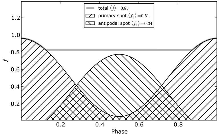
Figure 1.8: Observed flux fraction $f$ as a function of the rotation phase for PSR B0950+08. The following parameters were used: $\alpha=105.46^{\circ}$, $\beta=21.1^{\circ}$, $M=1.4\,{\rm M}_{\odot}$, $R=10\,{\rm km}$. The gravitational bending of light increases the flux ratio of the antipodal to primary spots almost two times ($0.85/0.5=1.7$) and also increases the antipodal to the primary flux ratio ($\sim 1.3$).

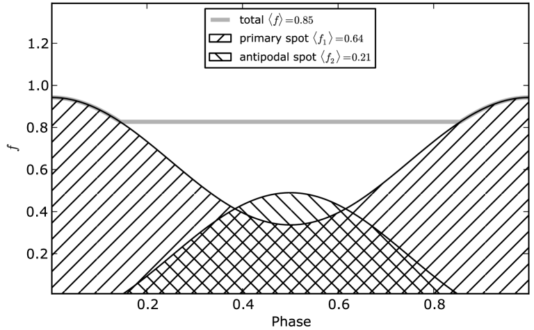
Figure 1.9: Observed flux fraction $f$ as a function of the rotation phase for PSR B1929+10. The following parameters were used: $\alpha=35.97$, $\beta=25.55^{\circ}$, $M=1.4\,{\rm M}_{\odot}$, $R=10\,{\rm km}$. The gravitational bending of light increases the observed flux fraction two times ($\left\langle f\right\rangle/\left\langle\cos i\right\rangle=1.98$) and also increases the flux ratio of the antipodal to primary spots almost seven times ($\sim 6.7$).

1.4.4 Observations

As we have shown in the previous sections, the blackbody fit to the X-ray observations allows us to directly obtain the surface temperature $T_{{\rm s}}$. Using the distance to pulsar $D$ and the luminosity of thermal emission $L_{{\rm BB}}$ we can estimate the area of spot $A_{{\rm bb}}$. In most cases, $A_{{\rm bb}}$ differs from the conventional polar cap area $A_{{\rm dp}}\approx 6.2\times 10^{4}P^{-1}\,{\rm m^{2}}$. We use parameter $b=A_{{\rm dp}}/A_{{\rm bb}}$ to describe the difference between $A_{{\rm dp}}$ and $A_{{\rm bb}}$.

Entire surface radiation and warm spot component (b<1)

In most cases the observed spot area $A_{{\rm bb}}$ is larger than the conventional polar cap area (see Table 1.4). We can distinguish two types of pulsars in this group, with $b\ll 1$ and $b\lesssim 1$.

The first type is associated with observations of a thermal emission from the entire stellar surface and can be used to test cooling models. Although the entire surface radiation is strongest for young pulsars ($\tau\lesssim 10$ kyr ), observation of this radiation is very difficult due to the strong nonthermal component. A common practice is to separately fit the nonthermal (PL) and thermal (BB) components. However, the temperature obtained in such a BB fit (without the PL component) is most likely overestimated (e.g. see PSR J2021+3651 in Table 1.4). The nonthermal luminosity of an aging neutron star decreases proportionally to its spin-down luminosity $L_{{\rm SD}}$, which is thought to drop with the star age as $L_{{\rm SD}}\propto\tau^{-m}$, where $m\simeq 2-4$ depends on the pulsar dipole breaking index (Zavlin, 2007b, ). As a pulsar becomes older, its surface temperature decreases. Depending on the model, a predicted temperature decrease in the early stages is gradual (the standard model) or rapid (the accelerated cooling scenario). For a number of middle-aged ($\tau\sim 100\,{\rm kyr}$) and some younger ($\tau\sim 10\,{\rm kyr}$) pulsars the thermal radiation from the entire stellar surface dominates the radiation at soft X-ray energies (e.g. PSR J0633+1746, PSR B1055-52, PSR J0821-4300, PSR B0656+14, PSR J0205+6449, PSR J2021+3651). However, the sample of pulsars is not sufficient to unambiguously identify the cooling scenario.

The second type is associated with observations of the warm spot area that is larger than the conventional polar cap area but still significantly less than the area of the star ($b\lesssim 1$). The age of pulsars in this group varies from very young ($\tau\sim 1\,{\rm kyr}$) to middle-aged ($\tau\sim 100\,{\rm kyr}$) neutron stars. There is one exception, namely PSR J1210-5226, which is very old ($\tau=105\,{\rm Myr}$) and can still be classified as a pulsar with the large warm spot component. Note, however, that the age of this pulsar is estimated using a characteristic value and if the pulsar period at birth is comparable with the current period then the age is highly overestimated (see, e.g. PSR J0821-4300). Furthermore, the fit to the X-ray spectrum was performed using only one thermal component and assuming no nonthermal radiation (PL). We believe that in many cases the size of the warm spot component and its temperature are overestimated by neglecting other sources of X-ray radiation, i.e. the nonthermal component and the hot spot radiation. The small number of observed X-ray photons in some cases prevents a full spectrum fit with all thermal and nonthermal components. Therefore, we need observations with better statistics so that the spectrum fit can be extended using more spectral components. The non-dipolar structure of the surface magnetic field may cause significant deviations from the spherical symmetry of the transport processes in the crust. The magnetic field slightly enhances heat transport along the magnetic lines, but strongly suppresses it in the perpendicular direction (Greenstein and Hartke,, 1983). Hence, the non-isothermality of the crust strongly depends on the geometry of the magnetic field (Geppert et al.,, 2004). The drastic difference of the crustal transport process causes significant differences in the surface temperature distribution (Page et al.,, 2006). Thus, the non-dipolar structure of the surface magnetic field can explain the existence of large warm spot components for young and middle-aged pulsars. We also suggested a mechanism of heating the surface adjacent to the polar cap (Szary et al.,, 2011). The model of such heating is also based on the assumption that the pulsar magnetic field near the stellar surface differs significantly from the pure dipole one. The calculations show that it is natural to obtain such a geometry of the magnetic field lines that allows pair creation in the closed field line region (see Figure 1.10).

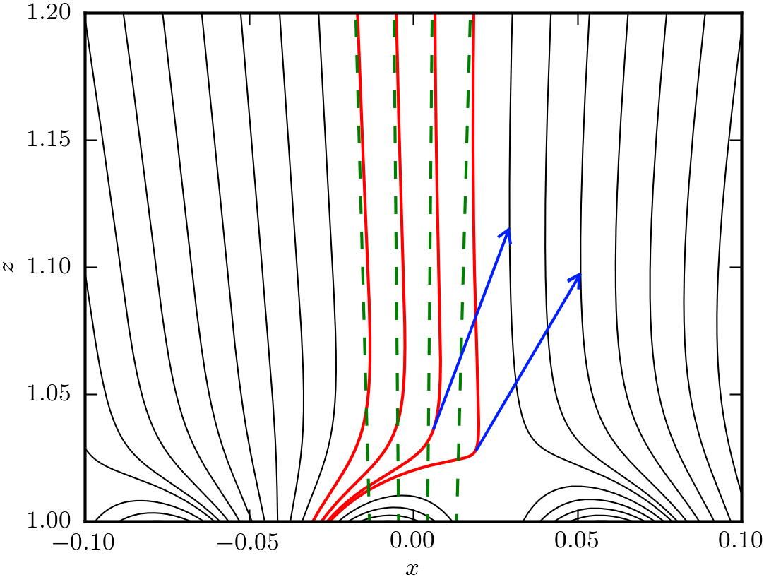
Figure 1.10: Cartoon of the magnetic field lines in the polar cap region. Red lines are open field lines and green dashed lines correspond to the dipole field. The blue arrows show the direction of the curvature photon emission.

The pairs move along the closed magnetic field lines and heat the surface beyond the polar cap on the opposite side of the star. In such a scenario the heating energy is generated in IAR, and hence the luminosity of such a warm spot is limited by the power of the outflowing particles (for more details see Section 5.1.2.3). In most cases the large size of the emitting area and its high temperature make it unlikely that the warm spot is related to the particles accelerated in IAR and is rather connected with the non-isothermality of the crust (e.g. PSR J1210-5226, PSR J1119-6127).

The hot spot component (b > 1)

In many cases the observed hot spot area $A_{{\rm bb}}$ is less than the conventional polar cap area ($b>1$). The temperature of the emitting area of these pulsars is usually higher than the temperature of the emitting area of pulsars with a warm spot component ($b<1$). The hot spot component is a natural consequence of the non-dipolar structure of the surface magnetic field (see Figure 1.10). In order to define an actual polar cap we need to follow the open field lines from the light cylinder up to the stellar surface by taking into account the non-dipolar structure of the surface magnetic field (see Figure 1.10), which can be estimated by the magnetic flux conservation law as $b=A_{{\rm dp}}/A_{{\rm bb}}$ = $B_{{\rm s}}/B_{{\rm d}}$. Thus, if $b\gg 1$ then $B_{{\rm s}}\gg B_{{\rm d}}$.

In neutron stars with positively charged polar caps (${\bf\Omega}\cdot{\bf B}<0$), the outflow of iron ions depends on the surface temperature and the surface binding energy (the so-called cohesive energy) (Cheng and Ruderman,, 1980; Jones,, 1986; Abrahams and Shapiro,, 1991; Gil et al.,, 2003). The cohesive energy of condensed matter increases with magnetic field strength (Medin and Lai,, 2007). If for a given strength of the surface magnetic field the temperature is below the so-called critical temperature $T_{{\rm crit}}$ the ions can tightly bind to the condensed surface and a polar gap can form (see Chapter 3 for details). Medin and Lai, (2008) calculated the dependence of the critical temperature (for a vacuum gap formation) on the strength of the surface magnetic field. In Figure 1.11 we present the positions of pulsars with derived surface temperature $T_{{\rm s}}$ and hot spot area $A_{{\rm bb}}$ on the $B_{{\rm s}}-T_{{\rm s}}$ diagram, where $B_{{\rm s}}$ is estimated as $B_{{\rm s}}=bB_{{\rm d}}$. The red line represents the dependence of the critical temperature $T_{{\rm crit}}$ on $B_{{\rm s}}$. We can see that in most cases the pulsars’ positions follow the $B_{{\rm s}}-T_{{\rm crit}}$ theoretical curve. Note that the Figure includes only pulsars with a visible hot spot component (old pulsars). For younger pulsars (with warm spot components) it is not possible to estimate the surface magnetic field. There are a few cases which do not coincide with the theoretical curve. We believe that they correspond to the observations of warm spot component but with the area of radiation smaller than the conventional polar cap area (e.g. due to reheating of the surface beyond the polar cap, see Section 1.4.4).

According to our model the actual surface temperature is almost equal to the critical value $T_{{\rm s}}\approx T_{{\rm crit}}$, which leads to the formation of the Partially Screened Gap (PSG) above the polar caps of a neutron star (Gil et al.,, 2003). The hot spot parameters derived from X-ray observations of isolated neutron stars are presented in Table 1.4.

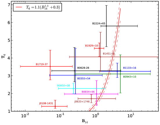
Figure 1.11: Diagram of the surface temperature ($T_{6}=T_{{\rm s}}/\left(10^{6}\,{\rm K}\right)$) vs. the surface magnetic field ($B_{14}=B_{{\rm s}}/\left(10^{14}\,{\rm G}\right)$). The red line represents the dependence of $T_{{\rm crit}}$ on $B_{14}$ according to Medin and Lai, (2008) and the dashed lines correspond to uncertainties in the calculations. The diagram includes all pulsars with $b>1$ with the exception of PSR J2043+2740, for which the blackbody fit was performed using a fixed radius (estimation of the surface magnetic field is not possible). Error bars correspond to $1\sigma$.

Table 1.4: Spectral properties of rotation-powered pulsars with detected blackbody X-ray components. The individual columns are as follows: (1) Pulsar name, (2) Spectral components required to fit the observed spectra, PL: power law, BB: blackbody, (3) Radius of the spot obtained from the blackbody fit $R_{{\rm bb}}$, (4) Surface temperature $T_{{\rm s}}$, (5) Surface magnetic field strength $B_{{\rm s}}$, (6) $b=A_{{\rm dp}}/A_{{\rm bb}}=B_{{\rm s}}/B_{{\rm d}}$, $A_{{\rm dp}}$ - conventional polar cap area, $A_{{\rm bb}}$ - actual polar cap area, (7) Bolometric luminosity of blackbody component $L_{{\rm BB}}$, (8) Bolometric efficiency $\xi_{{}_{{\rm BB}}}$, (9) Maximum nonthermal luminosity $L_{{\rm NT}}^{{}^{{\rm max}}}$, (10) Maximum nonthermal X-ray efficiency $\xi_{{}_{{\rm NT}}}^{{}^{{\rm max}}}$, (11) Best estimate of pulsar age or spin down age, (12) References, (13) Number of the pulsar. Nonthermal luminosity and efficiency were calculated in the $0.1-10\,{\rm keV}$ band. The maximum value was calculated with the assumption that the X-ray nonthermal radiation is isotropic. Pulsars are sorted by $b$ parameter (6).

Name	Spectrum	$R_{{\rm bb}}$	$T_{{\rm s}}$	$B_{{\rm s}}$	$b$	$\log L_{{\rm BB}}$	$\log\xi_{{}_{{\rm BB}}}$	$\log L_{{\rm X}}$	$\log\xi_{{}_{{\rm NT}}}^{{}^{{\rm max}}}$	$\tau$	Ref.	No.
			$\left(10^{6}{\rm K}\right)$	$\left(10^{14}{\rm G}\right)$		$\left({\rm erg\,s^{-1}}\right)$		$\left({\rm erg\,s^{-1}}\right)$
B1451–68	BB + PL	$14_{-12.3}^{+24.2}$ m	$4.1_{-0.81}^{+1.39}$	$1.36_{-1.18}^{+114}$	$418$	$29.27$	$-3.06$	$29.77$	$-2.56$	$42.5$ Myr	Po12	27
B0943+10	BB, PL	$12_{-7.7}^{+41.2}$ m	$3.1_{-1.07}^{+1.08}$	$4.99_{-4.72}^{+30.45}$	$126$	$28.40$	$-3.62$	$29.38$	$-2.64$	$4.98$ Myr	Zh05,Ka06	15
B1929+10	BB + PL	$28_{-3.8}^{+4.9}$ m	$4.5_{-0.45}^{+0.30}$	$1.26_{-0.35}^{+0.44}$	$122$	$30.06$	$-3.53$	$30.23$	$-3.36$	$3.10$ Myr	Mi08	43
B1133+16	BB, PL	$14_{-9.0}^{+10.5}$ m	$3.2_{-0.35}^{+0.46}$	$4.06_{-2.77}^{+31.79}$	$95.5$	$28.56$	$-3.38$	$29.52$	$-2.42$	$5.04$ Myr	Ka06	22
B0950+08	BB + PL	$42_{-26.6}^{+26.6}$ m	$2.3_{-0.29}^{+0.29}$	$0.23_{-0.15}^{+1.57}$	$47.9$	$28.92$	$-3.82$	$29.99$	$-2.76$	$17.5$ Myr	Za04	16
B2224+65	PL, BB	$28_{-18.0}^{+5.6}$ m	$5.8_{-1.16}^{+1.16}$	$2.00_{-0.61}^{+13.31}$	$38.6$	$30.51$	$-2.57$	$31.21$	$-1.87$	$1.12$ Myr	Hu12, Hu07b	47
J0633+1746	BB+BB+PL	$62_{-34.0}^{+34.0}$ m	$1.7_{-0.23}^{+0.23}$	$0.75_{-0.44}^{+2.92}$	$23.0$	$29.07$	$-5.44$	$30.24$	$-4.27$	$342$ kyr	Ja05	9
——		$11.17_{-1}^{+1}$ km	$0.5_{-0.1}^{+0.1}$			$31.67$	$-2.84$
B0834+06	BB + PL	$30_{-15.3}^{+56.4}$ m	$2.0_{-0.64}^{+0.75}$	$1.05_{-0.92}^{+3.19}$	$17.7$	$28.70$	$-3.41$	$28.70$	$-3.41$	$2.97$ Myr	Gi08	14
B0355+54	BB + PL	$92_{-53.6}^{+122.5}$ m	$3.0_{-1.06}^{+1.51}$	$0.27_{-0.22}^{+1.27}$	$15.9$	$30.40$	$-4.25$	$30.92$	$-3.73$	$564$ kyr	Mc07,Sl94	3
J0108–1431	BB + PL	$43_{-14.0}^{+24.0}$ m	$1.3_{-0.12}^{+0.35}$	$0.07_{-0.04}^{+0.08}$	$14.0$	$27.94$	$-2.82$	$28.57$	$-2.19$	$166$ Myr	Po12, Pa09	1
Continued on next page

Table 1.4 - continued from previous page Name Spectrum $R_{{\rm bb}}$ $T_{{\rm s}}$ $B_{{\rm s}}$ $b$ $\log L_{{\rm BB}}$ $\log\xi_{{}_{{\rm BB}}}$ $\log L_{{\rm X}}$ $\log\xi_{{}_{{\rm NT}}}^{{}^{{\rm max}}}$ $\tau$ Ref. No. $\left(10^{6}{\rm K}\right)$ $\left(10^{14}{\rm G}\right)$ $\left({\rm erg\,s^{-1}}\right)$ $\left({\rm erg\,s^{-1}}\right)$ B0628–28 BB + PL $64_{-49.7}^{+70.3}$ m $3.3_{-0.62}^{+1.31}$ $0.25_{-0.19}^{+4.88}$ $4.14$ $30.22$ $-1.94$ $30.22$ $-1.94$ $2.77$ Myr Te05, Be05 8 J2043+2740 BB + PL $358_{-153.2}^{+153.2}$ m $1.9_{-0.45}^{+0.45}$ $0.01_{-0.01}^{+0.02}$ $1.70$ $30.77$ $-3.98$ $31.41$ $-3.34$ $1.20$ Myr Be04 46 B1719–37 BB $237_{-122.5}^{+390.6}$ m $3.5_{-0.76}^{+0.91}$ $0.05_{-0.04}^{+0.17}$ $1.57$ $31.19$ $-3.32$ – – $345$ kyr Oo04 32 J1846–0258 BB + PL $306_{-153.2}^{+153.2}$ m $13.6_{-3.03}^{+3.03}$ – $0.686$ $34.06$ $-2.85$ $35.13$ $-1.78$ $0.73$ kyr Ng08, He03 39 B1055–52 BB+BB+PL $460_{-60.0}^{+60.0}$ m $1.8_{-0.06}^{+0.06}$ – $0.503$ $30.89$ $-3.59$ $30.91$ $-3.57$ $535$ kyr De05 18 $12.30_{-1}^{+2}$ km $0.8_{-0.03}^{+0.03}$ $32.62$ $-1.86$ J0538+2817 BB $666_{-38.3}^{+38.3}$ m $2.8_{-0.04}^{+0.05}$ – $0.330$ $31.97$ $-2.73$ – – $30.0$ kyr Mc03 6 J1809–1917 BB + PL $951_{-693.3}^{+920.2}$ m $2.0_{-0.35}^{+0.35}$ – $0.280$ $31.69$ $-4.56$ $31.57$ $-4.68$ $51.3$ kyr Ka07 36 J0821–4300 BB + BB $1.22_{-0.13}^{+0.13}$ km $6.3_{-0.19}^{+0.19}$ – $0.125$ $33.61$ $-0.91$ – – $3.70$ kyr Go10 11 —— $6.02_{-0.4}^{+0.4}$ km $3.2_{-0.10}^{+0.10}$ $33.86$ $-0.66$ B1951+32 BB + PL $2.20_{-0.80}^{+1.40}$ km $1.5_{-0.23}^{+0.23}$ – $0.110$ $31.95$ $-4.62$ $33.22$ $-3.35$ $107$ kyr Li05 44 B0833–45 BB + PL $1.61_{-0.15}^{+0.15}$ km $1.9_{-0.05}^{+0.05}$ – $0.091$ $32.12$ $-4.72$ $32.62$ $-4.22$ $11.3$ kyr Za07b 13 J1357–6429 BB + PL $1.91_{-0.38}^{+0.38}$ km $2.2_{-0.26}^{+0.26}$ – $0.034$ $32.50$ $-3.99$ $32.15$ $-4.35$ $7.31$ kyr Za07 25 J1210–5226 BB $1.23$ km $3.8$ – $0.033$ $33.04$ $1.51$ – – $102$ Myr Pa02 23 B1823–13 BB + PL $2.52_{-0.00}^{+0.00}$ km $1.6_{-0.07}^{+0.10}$ – $0.032$ $32.19$ $-4.27$ $31.78$ $-4.67$ $21.4$ kyr Pa08 38 B1916+14 BB, PL $800_{-100.0}^{+100.0}$ m $1.5_{-0.12}^{+0.12}$ – $0.028$ $31.07$ $-2.63$ $32.00$ $-1.71$ $88.1$ kyr Zh09 41 B1706–44 BB + PL $2.76_{-0.69}^{+0.69}$ km $2.2_{-0.20}^{+0.22}$ – $0.027$ $32.78$ $-3.76$ $32.16$ $-4.37$ $17.5$ kyr Go02 31

Table 1.4 - continued from previous page Name Spectrum $R_{{\rm bb}}$ $T_{{\rm s}}$ $B_{{\rm s}}$ $b$ $\log L_{{\rm BB}}$ $\log\xi_{{}_{{\rm BB}}}$ $\log L_{{\rm X}}$ $\log\xi_{{}_{{\rm NT}}}^{{}^{{\rm max}}}$ $\tau$ Ref. No. $\left(10^{6}{\rm K}\right)$ $\left(10^{14}{\rm G}\right)$ $\left({\rm erg\,s^{-1}}\right)$ $\left({\rm erg\,s^{-1}}\right)$ B2334+61 BB + PL $1.27_{-0.30}^{+0.45}$ km $2.1_{-0.76}^{+0.46}$ – $0.026$ $32.06$ $-2.73$ $31.55$ $-3.24$ $40.9$ kyr Mc06 48 B0656+14 BB+BB+PL $1.80_{-0.15}^{+0.15}$ km $1.2_{-0.03}^{+0.03}$ – $0.017$ $31.45$ $-3.13$ $30.26$ $-4.33$ $111$ kyr De05 10 —— $20.90_{-4}^{+3}$ km $0.7_{-0.01}^{+0.01}$ $32.74$ $-1.84$ J1119–6127 BB + PL $2.60_{-0.23}^{+1.38}$ km $3.1_{-0.26}^{+0.39}$ – $0.008$ $33.37$ $-3.00$ $32.95$ $-3.42$ $1.61$ kyr Go07, Ng12 20 J0205+6449 BB + PL $8.1$ km $1.7$ – $0.005$ $33.60$ $-3.83$ $33.10$ $-4.33$ $5.37$ kyr Sl04 2 J2021+3651 PL, BB $7.00_{-1.70}^{+4.00}$ km $2.4_{-0.30}^{+0.30}$ – $0.004$ $33.78$ $-2.75$ $34.36$ $-2.17$ $17.2$ kyr Va08,He04 45

Chapter 2 Model of a non-dipolar surface magnetic field

2.1 The magnetic field of neutron stars

Generally, the properties of pulsar radio emission support the assumption that the magnetic field of pulsars is purely dipolar at least in the radio emission region (Radhakrishnan and Cooke,, 1969). However, radio emission is generated at altitudes $R_{{\rm em}}$ of more than several stellar radii (e.g. Kijak and Gil, (1997), Kijak and Gil, (1998), Krzeszowski et al., (2009) and references therein). Thus, radio observations do not provide information about the structure of the magnetic field at the surface of the neutron star. On the other hand, strong non-dipolar surface magnetic fields have long been thought to be a necessary condition for pulsar activities, e.g. the vacuum gap model proposed by Ruderman and Sutherland, (1975) implicitly assumes that the radius of curvature of field lines above the polar cap should be about $10^{6}\,{\rm cm}$ in order to sustain pair production. This curvature is approximately $100$ times higher than that expected from a global dipolar magnetic field. Furthermore, to explain radiation from the Crab Nebula, the Crab pulsar should provide quite a dense stellar wind, as such a high particle multiplicity is not possible in a purely dipolar magnetic field.

There are several theoretical studies concerning the formation and evolution of the non-dipolar magnetic fields of neutron stars (e.g. Blandford et al., 1983; Krolik, 1991; Ruderman, 1991; Arons, 1993; Chen and Ruderman, 1993; Geppert and Urpin, 1994; Mitra et al., 1999; Page et al., 2006). According to Woltjer, (1964), the magnetic field in neutron stars results from the fossil field of the progenitor stars which is amplified during the collapse and remains anchored in the superfluid core of the neutron star. Several authors also noted that during the collapse (or shortly after) there is possible magnetic field generation in the external crust, for instance, by a mechanism like thermomagnetic instabilities (Blandford et al.,, 1983). Urpin et al., (1986) also showed that it is possible to form small-scale magnetic field anomalies in the neutron star crust with a typical size of the order of $100$ meters.

The soft X-ray observations of pulsars presented in Chapter 1 show non-uniform surface temperatures which can be attributed to small-scale magnetic anomalies in the crust. Further observational arguments in favour of the non-dipolar nature of the surface magnetic field can be found in many articles (e.g. Bulik et al., 1992; Thompson and Duncan, 1995; Bulik et al., 1995; Page and Sarmiento, 1996; Thompson and Duncan, 1996; Becker and Truemper, 1997; Cheng et al., 1998; Rudak and Dyks, 1999; Cheng and Zhang, 1999; Murakami et al., 1999; Tauris and Konar, 2001; Maciesiak et al., 2012).

2.2 Modelling of the surface magnetic field

In order to model a surface magnetic field we used the scenario proposed by Gil et al., (2002). In this scenario the magnetic field at the neutron star’s surface is non-dipolar in nature, which is due to superposition of the fossil field in the core and crustal field structures. To calculate the actual surface magnetic field described by superposition of the star-centred global dipole $\mathbf{d}$ and the crust-anchored dipole moment $\mathbf{m}$, let us consider the general situation presented in Figure 2.1

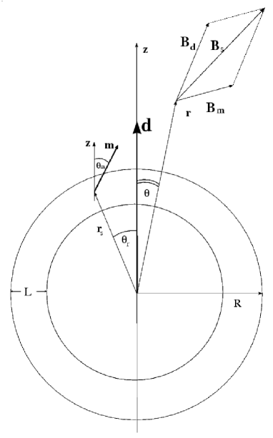
Figure 2.1: Superposition of the star-centred global magnetic dipole $\mathbf{d}$ and crust-anchored local dipole anomaly $\mathbf{m}$ located at $\mathbf{r_{s}}=(r_{s}\sim R,\,\theta=\theta_{r})$ and inclined to the $z$-axis by an angle $\theta_{m}$. The actual surface magnetic field at radius vector $\mathbf{r}=(r,\,\theta)$ is $\mathbf{B_{s}}=\mathbf{B_{d}}+\mathbf{B_{{\rm m}}}$, where $B_{d}=2d/r^{3}$, $B_{{\rm m}}=2m/|\mathbf{r}\mathbf{r_{s}}|^{3}$, $r$ is the radius and $\theta$ - is the polar angle. $R$ is the radius of the neutron star and L is the external crust thickness. Gil et al., (2002)

The actual surface magnetic field is a sum of the global magnetic dipole and crust-anchored local anomalies

$$\mathbf{B_{s}}=\mathbf{B_{d}}+\mathbf{B_{{\rm m}}}+...$$ (2.1)

Using the star-centred spherical coordinates with the $z$-axis directed along the global magnetic dipole moment we obtain:

$$\mathbf{B_{d}}=\left(\frac{2d\cos\theta}{r^{3}},\,\frac{d\sin\theta}{r^{3}},\,0\right),$$ (2.2)

$$\mathbf{B_{{\rm m}}}=\frac{3(\mathbf{r}-\mathbf{r_{s}})(\mathbf{m}\cdot(\mathbf{r}-\mathbf{r_{s}}))-\mathbf{m}|\mathbf{r}-\mathbf{r_{s}}|^{2}}{|\mathbf{r}-\mathbf{r_{s}}|^{5}}.$$ (2.3)

Here $\mathbf{r_{s}}=(r_{s},\,\theta_{r},\,\phi_{r})$, $\mathbf{m}=(m,\,\theta_{m},\,\phi_{m})$ and the spherical components of $\mathbf{B_{{\rm m}}}$ are explicitly given in Equation 2.7.

The global magnetic moment can be written as

$$d=\frac{1}{2}B_{{\rm p}}R^{3},$$ (2.4)

where $B_{{\rm p}}=6.4\times 10^{19}\left(P\dot{P}\right){}^{1/2}\,{\rm G}$ is the dipole component at the pole derived from pulsar spin-down energy loss.

The crust-anchored local dipole moment is

$$m=\frac{1}{2}B_{{\rm m}}\Delta R^{3},$$ (2.5)

where $\Delta R\sim 0.05R<L$ and $L\sim 10^{5}\,{\rm cm}$ is the characteristic crust dimension (for $R=10^{6}\,{\rm cm}$). For these values a local anomaly can significantly influence the surface magnetic field ($B_{{\rm m}}>B_{{\rm d}}$) if $m/d>10^{-4}$.

The system of differential equations for a field line of the vector field $\mathbf{B=}\left(B_{r},\,B_{\theta},\,B_{\phi}\right)$ in spherical coordinates can be written as

$$\begin{cases}\frac{{\rm d}\theta}{{\rm d}r}&=\frac{B_{\theta}}{rB_{r}}\\ \frac{{\rm d}\phi}{{\rm d}r}&=\frac{B_{\phi}}{r\sin(\theta)B_{r}}.\end{cases}$$ (2.6)

The solution of these equations, with the initial conditions $\theta_{0}=\theta(r=R)$ and $\phi_{0}$=$\phi$(r=R) determining a given field line at the stellar surface, describes the parametric equation of the magnetic field lines. The spherical components of $\mathbf{B_{{\rm m}}}$ can be written in the following form

$$\begin{split}B_{r}^{m}&=-\frac{1}{D^{2.5}}\left(3Tr_{r}^{s}-3Tr+Dm_{r}\right),\\ B_{\theta}^{m}&=-\frac{1}{D^{2.5}}\left(3Tr_{\theta}^{s}+Dm_{\theta}\right),\\ B_{\phi}^{m}&=-\frac{1}{D^{2.5}}\left(3Tr_{\phi}^{s}+Dm_{\phi}\right).\end{split}$$ (2.7)

Here

$$D=r_{s}^{2}+r^{2}-2r_{s}r\left(\sin\theta_{r}\sin\theta\cos\left(\phi-\phi_{r}\right)+\cos\theta_{r}\cos\theta\right),$$ (2.8)

and

$$T=m_{r}r-\left(m_{r}r_{r}^{s}+m_{\theta}r_{\theta}^{s}\right).$$ (2.9)

According to the geometry presented in Figure 2.1, the components of the radius vector of the origin of the crust-anchored local dipole anomaly can be written as

$$\begin{split}r_{r}^{s}&=r_{s}\left(\sin\theta_{r}\sin\theta\cos\left(\phi-\phi_{r}\right)+\cos\theta_{r}\cos\theta\right),\\ r_{\theta}^{s}&=r_{s}\left(\sin\theta_{r}\cos\theta\cos\left(\phi-\phi_{r}\right)+\cos\theta_{r}\sin\theta\right),\\ r_{\phi}^{s}&-r_{s}\sin\theta_{r}\sin\left(\phi-\phi_{r}\right).\end{split}$$ (2.10)

The components of the local dipole anomaly are

$$\begin{split}m_{r}&=m\left(\sin\theta_{m}\sin\theta\cos\left(\phi-\phi_{m}\right)+\cos\theta_{m}\cos\theta\right),\\ m_{\theta}&=m\left(\sin\theta_{m}\cos\theta\cos\left(\phi-\phi_{m}\right)+\cos\theta_{m}\sin\theta\right),\\ m_{\phi}&=-m\sin\theta_{m}\sin\left(\phi-\phi_{m}\right).\end{split}$$ (2.11)

Finally, we obtain the system of differential equations from Equation 2.6 by substitutions $B_{r}=B_{r}^{d}+B_{r}^{m}$, $B_{\theta}=B_{\theta}^{d}+B_{\theta}^{m}$ and $B_{\phi}=B_{\phi}^{d}+B_{\phi}^{m}$ (Equations 2.2 and 2.7)

$$\frac{{\rm d}\theta}{{\rm d}r}=\frac{B_{\theta}^{d}+B_{\theta}^{m}}{r\left(B_{r}^{d}+B_{r}^{m}\right)}\equiv\Theta_{1},$$ (2.12)

$$\frac{{\rm d}\phi}{{\rm d}r}=\frac{B_{\phi}^{m}}{r\left(B_{r}^{d}+B-r^{m}\right)\sin\theta}\equiv\Phi_{1}.$$ (2.13)

2.3 Curvature of magnetic field lines

As Curvature Radiation (CR) may play a decisive role in radiation processes, it is important to calculate the curvature (or curvature radius) for each field line. The curvature $\rho_{c}=1/\Re$ of field lines (where $\Re$ is the radius of curvature) is calculated as (Gil et al.,, 2002)

$$\rho_{c}=\left(\frac{{\rm d}s}{{\rm d}r}\right)^{-3}\left|\left(\frac{{\rm d}^{2}\mathbf{r}}{{\rm d}r^{2}}\frac{{\rm d}s}{{\rm d}r}-\frac{{\rm d}\mathbf{r}}{{\rm d}r}\frac{{\rm d}^{2}s}{{\rm d}r^{2}}\right)\right|,$$ (2.14)

where

$$\frac{{\rm d}s}{{\rm d}r}=\sqrt{\left[1+r^{2}\Theta_{1}^{2}+r^{2}\Phi_{1}^{2}\sin^{2}(\theta)\right]}.$$ (2.15)

Thus, the curvature can be written in the form

$$\rho_{c}=\left(S_{1}\right)^{-3}\left(J_{1}^{2}+J_{2}^{2}+J_{3}^{2}\right)^{1/2},$$ (2.16)

where

$$\begin{split}J_{1}=&X_{2}S_{1}-X_{1}S_{2},\\ J_{2}=&Y_{2}S_{1}-Y_{1}S_{2},\\ J_{3}=&Z_{2}S_{1}-Z_{1}S_{2},\\ X_{1}=&\sin\theta\cos\phi+r\Theta_{1}\cos\theta\cos\phi-r\Phi_{1}\sin\theta\sin\phi,\\ Y_{1}=&\sin\theta\sin\phi+r\Theta_{1}\cos\theta\sin\phi-r\Phi_{1}\sin\theta\cos\phi,\\ Z_{1}=&\cos\theta-r\Theta_{1}\sin\theta,\\ X_{2}=&\left(2\Theta_{1}+r\Theta_{2}\right)\cos\theta\cos\phi-\left(2\Phi_{1}+r\Phi_{2}\right)\sin\theta\sin\phi-\\ &r\left(\Theta_{1}^{2}+\Phi_{1}^{2}\right)\sin\theta\cos\phi+2r\Theta_{1}\Phi_{1}\cos\theta\sin\phi,\\ Y_{2}=&\left(2\Theta_{1}+r\Theta_{2}\right)\cos\theta\sin\phi+\left(2\Phi_{1}+r\Phi_{2}\right)\sin\theta\cos\phi-\\ &r\left(\Theta_{1}^{2}+\Phi_{1}^{2}\right)\sin\theta\sin\phi+2r\Theta_{1}\Phi_{1}\cos\theta\cos\phi,\\ Z_{2}=&-\Theta_{1}\sin\theta-\Theta_{1}\sin\theta-r\Theta_{2}\sin\theta-r\Theta_{1}^{2}\cos\theta,\\ S_{1}=&\sqrt{1+r^{2}\Theta_{1}^{2}+r^{2}\Phi_{1}^{2}\sin^{2}\theta},\\ S_{2}=&S_{1}^{-1}\left(t\Theta_{1}^{2}+r^{2}\Theta_{1}\Theta_{2}+r\Phi_{1}^{2}\sin^{2}\theta+r^{2}\Phi_{1}\Phi_{2}\sin^{2}\theta+r^{2}\Theta_{1}\Phi_{1}^{2}\sin\theta\cos\theta\right),\\ \Theta_{2}\equiv&\frac{{\rm d}\Theta_{1}}{{\rm d}r},\\ \Phi_{2}\equiv&\frac{{\rm d}\Phi_{1}}{{\rm d}r}.\end{split}$$ (2.17)

2.3.1 Numerical calculation of the curvature

Let us note that when evaluating Equation 2.6 it was assumed that $\sin\theta\neq 0$. Thus $\Phi_{1}$ and $\Phi_{2}$ are undefined for $\theta=0$. Figure 2.2 presents the first and second derivative ($\Phi_{1}$, $\Phi_{2}$) of the $\phi$-coordinate of a magnetic field line with respect to the $r$-coordinate for a magnetic field structure with $B_{\phi}\neq 0$.

The singularity in Equation 2.6 may result in an overestimation of curvature of field lines that cross the $\theta=0$ plane for a complex structure of the surface magnetic field. To solve this problem, and in addition to the analytical approach, the numerical calculation of the curvature of magnetic field lines was implemented.

Let us consider three consecutive points of the given magnetic field line $A$, $B$, $C$ (see Figure 2.3).

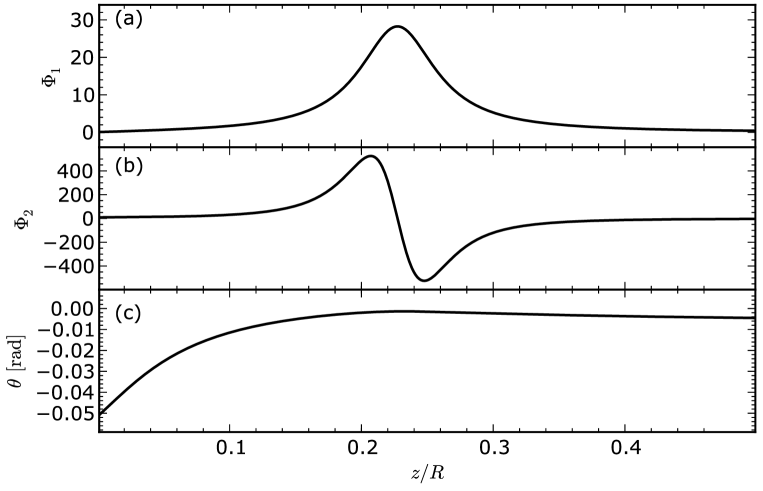
Figure 2.2: Plot of the first and second derivative of the $\phi$-coordinate of the magnetic field line with respect to the $r$-coordinate vs. the distance from the stellar surface. Values were calculated using the approach described in Section 2.3. Panels (a) and (b) show the first and second derivative of the $\phi$-coordinate while panel (c) shows the $\theta$-coordinate of the magnetic field line.

Figure 2.3: For any given three points ($A$, $B$, $C$) we can always find a common plane. We use the following transformations to achieve this: (I) shift the origin of the system to point $A$ (prime), (II) rotate the shifted system by an angle $\varsigma_{y}$ around the $y^{\prime}$–axis and by an angle $\varsigma_{x}$ around the $x^{\prime\prime}$-axis (double prime). After these transformations the $z^{\prime\prime}$-axis will be aligned with normal vector $\hat{{\bf N}}$ and all points will lie in the $x^{\prime\prime}y^{\prime\prime}$-plane of such a system of coordinates.

To calculate curvature (or radius of curvature) in point $B$ we can use the following procedure:

• simplify the 3-D problem to 2-D by finding a common plane for all three points

  • move the origin of the coordinate system to point $A$

  • rotate the coordinate system to align the z-axis with the normal vector to the common plane of all three points ($A$, $B$, $C$)

• calculate the radius of the circle passing through all three points (in a 2-D coordinate system)

3-D to 2-D transition

To simplify the calculations we shift the origin of the coordinate system so that point $A$ will be the origin of the new system:

$$A^{\prime} = \left(0,\,0,\,0\right);$$

$$B^{\prime} = \left(B_{1}-A_{1},\,B_{2}-A_{2},\,B_{3}-A_{3}\right);$$ (2.18)

$$C^{\prime} = \left(C_{1}-A_{1},\,C_{2}-A_{2},\,C_{3}-A_{3}\right).$$

The unit normal vector to the plane enclosing all three points ($A^{\prime}$, $B^{\prime}$, $C^{\prime}$) can be calculated as

$$\hat{{\bf N}}=\frac{{\bf b}\times{\bf c}}{\left|{\bf b}\times{\bf c}\right|}=\left(N_{1},\,N_{2},\,N_{3}\right),$$ (2.19)

where ${\bf b}=\left(B_{1}^{\prime},\,B_{2}^{\prime},\,B_{3}^{\prime}\right)$ and ${\bf c}=\left(C_{1}^{\prime},\,C_{2}^{\prime},\,C_{3}^{\prime}\right)$.

The next step is to rotate the shifted coordinate system to align the $z^{\prime}$-axis with normal vector $\hat{{\bf N}}$. In the new system all three points will lie in the $x^{\prime\prime}y^{\prime\prime}$-plane. In our calculations we rotate the shifted system by an angle $\varsigma_{y}$ around the $y^{\prime}$-axis, $R_{y}\left(\varsigma_{y}\right)$, and a rotation by an angle $\varsigma_{x}$ around the $x^{\prime\prime}$-axis, $R_{x}\left(\varsigma_{x}\right)$. The final rotation matrix can be written as

$$R_{yx}=R_{y}\left(\varsigma_{y}\right)R_{x}\left(\varsigma_{x}\right)=\left[\begin{array}[]{ccc}\cos\varsigma_{y}&\sin\varsigma_{x}\sin\varsigma_{y}&\sin\varsigma_{y}\cos\varsigma_{x}\\ 0&\cos\varsigma_{x}&-\sin\varsigma_{x}\\ -\sin\varsigma_{y}&\cos\varsigma_{y}\sin\varsigma_{x}&\cos\varsigma_{y}\cos\varsigma_{x}\end{array}\right]$$ (2.20)

The Euler angles for these rotations can be calculated as

$\varsigma_{x}={\rm atan2}\left(N_{2},N_{3}\right).$

$$\begin{array}[]{c}\varsigma_{y}=\begin{cases}\arctan\left(-\frac{N_{1}}{N_{3}}\cos\varsigma_{x}\right)&{\rm if\ }N_{3}\neq 0\\ \arctan\left(-\frac{N_{1}}{N_{2}}\sin\varsigma_{x}\right)&{\rm if\ }N_{2}\neq 0\\ \frac{\pi}{2}&{\rm if\ }N_{2}=0\ {\rm and}\ N_{3}=0\end{cases}\end{array}$$ (2.21)

Finally, we can write the components of all three points in our new (shifted and double-rotated) system of coordinates as follows

$$A^{\prime\prime} = R_{yx}A^{\prime}=\left(0,\,0,\,0\right);$$

$$B^{\prime\prime} = R_{yx}B^{\prime}=\left(B_{1}^{\prime\prime},\,B_{2}^{\prime\prime},\,0\right);$$ (2.22)

$$C^{\prime\prime} = R_{yx}C^{\prime}=\left(C_{1}^{\prime\prime},\,C_{2}^{\prime\prime},\,0\right).$$

Circle passing through 3 points (Bourne,, 2012)

Finding the radius of the circle passing through three consecutive points of a given magnetic field line ($A=\left(0,\,0\right)$, $B=\left(B_{1},\,B_{2}\right)$, $C=\left(C_{1},\,C_{2}\right)$) is an exact method for finding the radius of curvature $\Re$ and hence the curvature $\rho=1/\Re$ of this line. Note that for simplicity’s sake we hereafter describe points without double prime notation but they refer to coordinates in the shifted and double-rotated system of coordinates (e.g. $B=\left(B_{1},\,B_{2}\right)=\left(B_{1}^{\prime\prime},\,B_{2}^{\prime\prime}\right)$).

Slope $m_{1}$ of the line joining $A$ to $B$ and slope $m_{2}$ of the line joining $B$ to $C$ (see Figure 2.4) are given by

$$\begin{split}m_{1}=&\frac{\Delta y}{\Delta x}=\frac{B_{2}}{B_{1}},\\ m_{2}=&\frac{\Delta y}{\Delta x}=\frac{C_{2}-B_{2}}{C_{1}-B_{1}}.\end{split}$$ (2.23)

In general, the centre of the circle passing through our points is given by

$$\begin{split}x_{c}=&\frac{m_{1}m_{2}\left(A_{2}-C_{2}\right)+m_{2}\left(A_{1}-B_{1}\right)-m_{1}\left(B_{1}-C_{1}\right)}{2\left(m_{2}-m_{1}\right)},\\ y_{c}=&\frac{1}{m_{1}}\left(x_{c}-\frac{A_{1}+B_{1}}{2}\right)+\frac{A_{2}+B_{2}}{2}.\end{split}$$ (2.24)

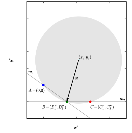
Figure 2.4: The radius of curvature $\Re$ of the magnetic field line at a given point $B$ can be calculated as the radius of the circle passing through this and the neighbouring two points ($A$, $C$). The system of coordinates was moved and double-rotated so that $A$ is in its origin and all points lie in the $x^{\prime\prime}y^{\prime\prime}$-plane. The slopes of the lines joining $A$ to $B$ and $B$ to $C$ are described by Equation 2.23.

Since point $A$ is in the centre of the coordinate system we can simplify these formulas as follows

$$\begin{split}x_{c}=&\frac{2\,B_{1}^{2}B_{2}-2\,B_{1}B_{2}C_{1}+B_{2}C_{1}^{2}-B_{2}C_{2}^{2}-\left(B_{1}^{2}-B_{2}^{2}\right)C_{2}}{2\,\left(B_{1}C_{2}-B_{2}C_{1}\right)},\\ y_{c}=&\frac{B_{2}^{2}-\left(B_{2}-2\,x_{c}\right)B_{1}}{2\,B_{2}}.\end{split}$$ (2.25)

Finally, we can calculate the radius of curvature simply by finding the distance between the centre of the circle and any of the points on the circle (we have chosen point $A$)

$$\Re=\frac{1}{\rho}=\sqrt{x_{c}^{2}+y_{c}^{2}}.$$ (2.26)

In this thesis we consider complex structures of the surface magnetic field, thus the numerical method presented above was used in all the calculations of curvature. The analytical approach may result in an overestimation of curvature for points with $\theta\approx 0$ (see Figure 2.5).

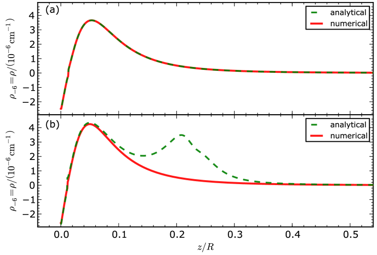
Figure 2.5: Curvature of the magnetic field lines vs. the height above the stellar surface calculated using the analytical approach described in Section [2.3] (green lines) and the numerical approach presented above (red lines). Panel (a) corresponds to the magnetic field line which has no $\phi$ component, while panel (b) corresponds to a more general scenario i.e. the nonzero $\phi$ component of the magnetic field line. As can be seen, the analytical approach is not valid for every case. This is caused by the undefined value of the $\phi$ derivative for $\theta=0$ (see Equation [2.6]). Here $\rho_{-6}=1/\Re_{6}=\rho/\left(10^{-6}\,{\rm cm}^{-1}\right)$ and $\Re_{6}=\Re/\left(10^{6}\,{\rm cm}\right)$.

2.4 Simulation results

In this section we model the surface non-dipolar magnetic field structure for some pulsars. Note that we can estimate the size of the polar cap and the strength of the surface magnetic field only for pulsars with an observed hot spot (see Section 1.4.4). Here we present only pulsars listed in Table 3.1.

We use spherical coordinates $\left(r,\,\theta,\,\phi\right)$ to describe the location and orientation of crust-anchored local anomalies. The parameters of anomalies are as follows: ${\bf r_{a}}=\left(r_{a},\,\theta_{a},\,\phi_{a}\right)$ is a radius vector which points to the location of the anomaly and ${\bf m_{a}}=\left(m_{a},\,\theta_{a}\,,\phi_{a}\right)$ is its dipole moment. The value of $m_{a}$ is measured in units of the global dipole moment $d$, i.e. the moment which corresponds to the pulsar’s global magnetic field. In the Figures showing a possible non-dipolar structure (e.g. Figure 2.6, 2.9, 2.12) the dashed lines correspond to the dipolar configuration of the magnetic field lines, while the solid lines correspond to the actual magnetic field lines (taking into account the crust-anchored anomalies). Green and red lines represent the open magnetic field lines for dipolar and non-dipolar structures, respectively.

2.4.1 PSR B0628-28

Pulsar B0628-28, a bright radio pulsar, was discovered by Large et al., (1969) during a pulsar search at 408 MHz. The pulsar period $P\approx 1.24\,{\rm s}$ and its first derivative $\dot{P}_{-15}\approx 7.1$ result in a dipolar component of magnetic field $B_{{\rm d}}=6\times 10^{12}\,{\rm G}$ and a characteristic age $\tau_{c}\approx 2.8\,{\rm Myr}$, which makes it a typical, old pulsar. The large distance to this pulsar $D=1.44\,{\rm kpc}$ (evaluated using the Galactic free electron density model of Cordes and Lazio,, 2002) makes it impossible to use the parallax method to determine the distance with better accuracy.

PSR B0628-28 is one of the longest period pulsars among those detected in X-rays. The pulsar was first detected in the X-ray band by ROSAT and then later observed with both the Chandra and XMM-Newton. Observations with the Chandra revealed no pulsations, while the XMM-Newton observations revealed pulsations with a period consistent with the period of radio emission (Tepedelenlıoǧlu and Ögelman,, 2005). The inconsistency of the observations is a reflection of the fact that the pulsar is detectable just at the threshold of sensitivity of both the observatories. The two-component spectral fit (BB+PL) shows that both the nonthermal and thermal components have a comparable luminosity (at least if we assume that the nonthermal radiation is isotropic, see Table 1.2). PSR B0628-28 is characterised by one of the largest X-ray efficiencies among the observed pulsars $\xi_{{\rm BB}}\approx\xi_{{\rm NT}}^{{}^{{\rm max}}}\approx 10^{-2}$.

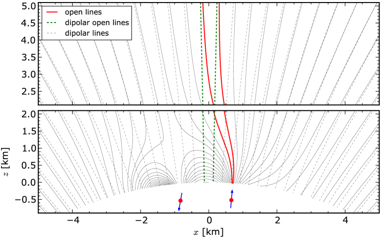
Figure 2.6: Possible non-dipolar structure of the magnetic field lines of PSR B0628-28. The structure was obtained using two crust anchored anomalies located at: ${\bf r_{1}}=\left(0.95R,\,4^{\circ},\,0^{\circ}\right)$, ${\bf r_{2}}=\left(0.95R,\,5^{\circ},\,180^{\circ}\right)$, with the dipole moments ${\bf m_{1}}=\left(4.5\times 10^{-3}d,\,5^{\circ},\,0^{\circ}\right)$, ${\bf m_{2}}=\left(4.5\times 10^{-3}d,\,170^{\circ},\,180^{\circ}\right)$ respectively (blue arrows). The influence of the anomalies is negligible at distances $D\gtrsim 2R$, where $B_{{\rm m}}/B_{{\rm d}}\approx m/d=4.5\times 10^{-3}$ (top panel). For more details on the polar cap region see Figure 2.7.

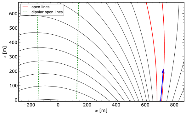
Figure 2.7: Zoom of the polar cap region of PSR B0628-28. See Figure 2.6 for a description.

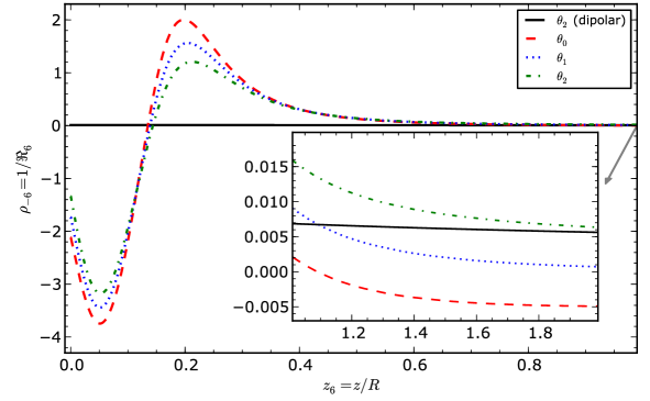
Figure 2.8: Dependence of a curvature of the open magnetic field lines on the distance from the stellar surface for PSR B0628-28. The distance is in units of the stellar radius $z_{6}=z/R$ and the curvature of the magnetic field lines is $\rho_{-6}=1/\Re_{6}=\rho/\left(10^{-6}\,{\rm cm}^{-1}\right)$.

2.4.2 PSR J0633+1746

Geminga was discovered in 1972 as a $\gamma$-ray source by Fichtel et al., (1975). The visual magnitude of the pulsar was estimated by Bignami et al., (1987) to be of the order of $\sim 25.5^{{}^{{\rm mag}}}$. The pulse modulation was discovered in X-rays (Halpern and Holt,, 1992), in $\gamma$-rays, and at optical wavelengths (Shearer et al.,, 1998). Geminga has been determined to be a relatively old ($\tau=342\,{\rm kyr}$) radio-quiet pulsar with a period $P=237\,{\rm ms}$. The distance to the pulsar $D=0.16\,{\rm kpc}$, evaluated using the parallax method, makes it the closest pulsar with available X-ray data.

The pulsar exhibits one of the weakest radio luminosities known and a cutoff at frequencies higher than about $100\,{\rm MHz}$. The model presented by Gil et al., (1998) explains this weak radio emission with absorption by the magnetised relativistic plasma inside the light cylinder. As the exact model of radio emission is still unknown (see Section Radio emission), it is difficult to verify if this weak radio emission is a result of absorption or the absence of coherent radio emission.

The three-component fit to the X-ray spectrum (PL+BB+BB, see Table 1.4) reveals the hot spot component with a size that is considerably smaller than the conventional polar cap size ($b\approx 23$). The entire surface temperature $T_{{\rm s}}=0.5\,{\rm MK}$ is consistent with the theoretical value predicted by the cooling model.

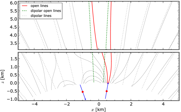
Figure 2.9: Possible non-dipolar structure of the magnetic field lines of PSR J0633+1746. The structure was obtained using two crust anchored anomalies located at: ${\bf r_{1}}=\left(0.95R,\,3^{\circ},\,0^{\circ}\right)$, ${\bf r_{2}}=\left(0.95R,\,6^{\circ},\,180^{\circ}\right)$, with the dipole moments ${\bf m_{1}}=\left(5.5\times 10^{-3}d,\,10^{\circ},\,0^{\circ}\right)$, ${\bf m_{2}}=\left(5.5\times 10^{-3}d,\,160^{\circ},\,0^{\circ}\right)$ respectively (blue arrows). The influence of the anomalies is negligible at distances $D\gtrsim 3.1R$, where $B_{{\rm m}}/B_{{\rm d}}\approx m/d=5.5\times 10^{-3}$ (top panel). For more details on the polar cap region see Figure 2.10.

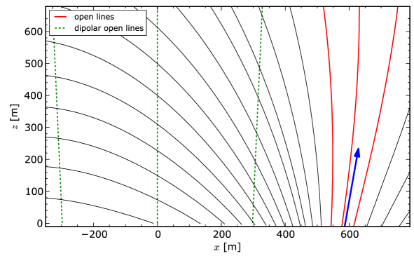
Figure 2.10: Zoom of the polar cap region of PSR J0633+1746. See Figure 2.9 for a description.

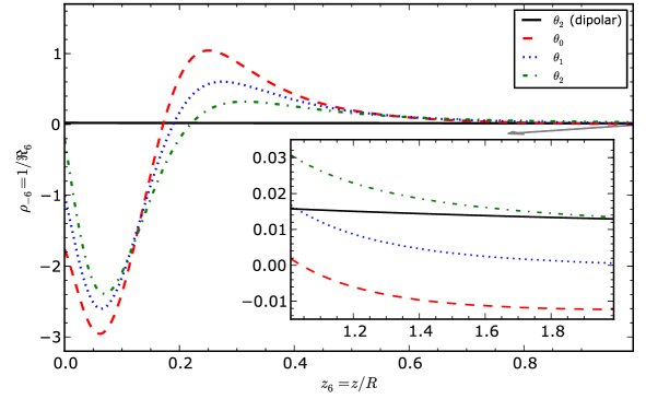
Figure 2.11: Dependence of a curvature of the open magnetic field lines on the distance from the stellar surface for PSR J0633+1746. The distance is in units of the stellar radius $z_{6}=z/R$ and the curvature of the magnetic field lines is $\rho_{-6}=1/\Re_{6}=\rho/\left(10^{-6}\,{\rm cm}^{-1}\right)$.

2.4.3 PSR B0834+06

The bright radio emission of PSR B0834+06 shows frequent nulls (nearly $9\%$ of the pulses is absent, see Rankin and Wright,, 2008) . With a relatively long rotational period $P=1.27\,{\rm s}$ and $\dot{P}_{-15}\approx 7.1$ (Taylor et al.,, 2000), its inferred physical properties, e.g. $B_{{\rm d}}=3\times 10^{12}\,{\rm G}$, are close to the average. The characteristic age $\tau_{c}=2.97\,{\rm Myr}$ implies that the pulsar should be categorised as an old pulsar. The distance to the pulsar, estimated as $D=0.64\,{\rm kc}$, was derived from its dispersion measure using the Galactic free-electron density model of Cordes and Lazio,, 2002. Weltevrede et al., (2006) suggest a drift of subpulses, but the estimated value of a subpulse separation is larger than the pulse width. Despite the fact that the geometry based on the carousel model could be fitted to the observations, there is no clear evidence for a drift of emission between the components of the pulsar (Rankin and Wright,, 2007).

The pulsar was detected in X-ray by Gil et al., (2008) with a total of $70$ counts from over $50\,{\rm ks}$ exposure time. Because of the low statistical quality of the X-ray data, it was not possible to constrain the absorbing column density $N_{H}$. The two-component spectral fit (BB + PL), as presented in this thesis, was performed using the assumption that both the thermal and nonthermal fluxes are of the same order.

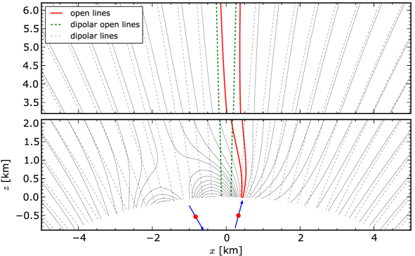
Figure 2.12: Possible non-dipolar structure of the magnetic field lines of PSR B0834+06. The structure was obtained using two crust anchored anomalies located at: ${\bf r_{1}}=\left(0.95R,\,2^{\circ},\,0^{\circ}\right)$, ${\bf r_{2}}=\left(0.95R,\,5^{\circ},\,180^{\circ}\right)$, with the dipole moments ${\bf m_{1}}=\left(3\times 10^{-3}d,\,15^{\circ},\,0^{\circ}\right)$, ${\bf m_{2}}=\left(3\times 10^{-3}d,\,150^{\circ},\,0^{\circ}\right)$ respectively (blue arrows). The influence of the anomalies is negligible at distances $D\gtrsim 3.2R$, where $B_{{\rm m}}/B_{{\rm d}}\approx m/d=3\times 10^{-3}$ (top panel). For more details on the polar cap region see Figure 2.13.

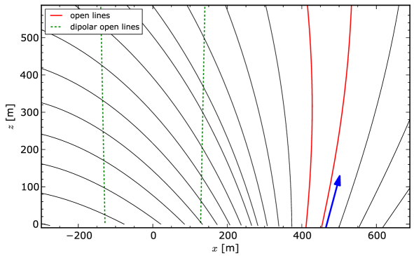
Figure 2.13: Zoom of the polar cap region of PSR B0834+06. See Figure 2.12 for a description.

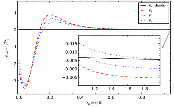
Figure 2.14: Dependence of a curvature of the open magnetic field lines on the distance from the stellar surface for PSR B0834+06. The distance is in units of stellar radius ($z_{6}=z/R$) and the curvature of the magnetic field lines is $\rho_{-6}=1/\Re_{6}=\rho/\left(10^{-6}\,{\rm cm}^{-1}\right)$.

2.4.4 PSR B0943+10

Pulsar B0943+10 is a relatively old pulsar with a characteristic age of $\tau_{c}=4.98\,{\rm Myr}$. The pulsar period $P=1.1\,{\rm s}$ and its first derivative $\dot{P}_{-15}\approx 3.5$ result in the dipolar component of a magnetic field $B_{{\rm d}}=4.0\times 10^{12}\,{\rm G}$. Using the Galactic free-electron density model of Cordes and Lazio,, 2002, we can estimate the distance to the pulsar $D=0.63\,{\rm kpc}$.

PSR B0943+10 is a well-known example of a pulsar exhibiting both the mode changing and subpulse drifting phenomenon. Strong, regular subpulse drifting is observed only in radio-bright mode, and only hints of the modulation feature have been found in the radio-quiescent mode. Very recent results presented by Hermsen et al., (2013) show synchronous switching in the radio and X-ray emission properties. When the pulsar is in a radio-bright mode, the X-rays exhibit only an unpulsed component. On the other hand, when the pulsar is in a radio-quiet mode, the flux of X-rays is doubled and a pulsed component is also visible.

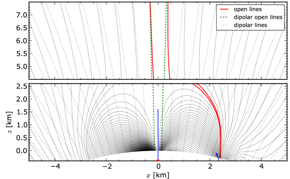
Figure 2.15: Possible non-dipolar structure of the magnetic field lines of PSR B0943+10. The structure was obtained using two crust anchored anomalies located at: ${\bf r_{1}}=\left(0.96R,\,0^{\circ},\,0^{\circ}\right)$, ${\bf r_{2}}=\left(0.96R,\,15^{\circ},\,0^{\circ}\right)$, with the dipole moments ${\bf m_{1}}=\left(2.0\times 10^{-2}d,\,180^{\circ},\,0^{\circ}\right)$, ${\bf m_{2}}=\left(6\times 10^{-3}d,\,20^{\circ},\,180^{\circ}\right)$ respectively (blue arrows). The influence of the anomalies is negligible at distances $D\gtrsim 4.5R$, where $B_{{\rm m}}/B_{{\rm d}}\approx m/d=2\times 10^{-2}$ (top panel). For more details on the polar cap region see Figure 2.16.

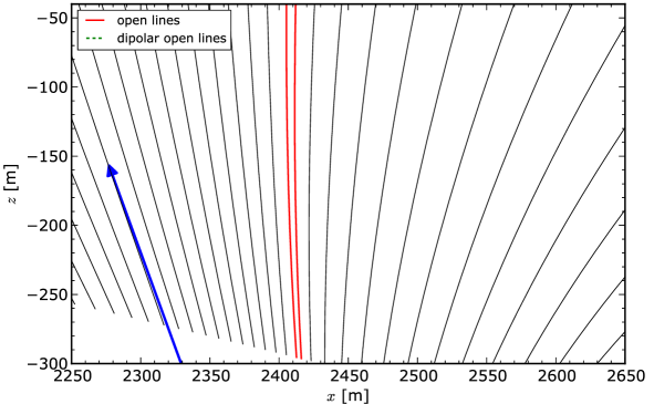
Figure 2.16: Zoom of the polar cap region of PSR B0943+10. See Figure 2.15 for a description.

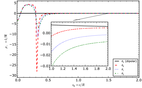
Figure 2.17: Dependence of a curvature of the open magnetic field lines on the distance from the stellar surface for PSR B0943+10. The distance is in units of stellar radius ($z_{6}=z/R$) and the curvature of the magnetic field lines is $\rho_{-6}=1/\Re_{6}=\rho/\left(10^{-6}\,{\rm cm}^{-1}\right)$.

2.4.5 PSR B0950+08

Pulsar B0950+08 is one of the strongest pulsed radio sources in the metre wavelength range. The pulsar radiation also exhibits an interpulse located at $152^{\circ}$ from the main pulse (Smirnova and Shabanova,, 1992). Based on the period $P=1.1\,{\rm s}$ and its first derivative $\dot{P}_{-15}\approx 3.5$, we can estimate the pulsar’s characteristic age $\tau_{c}=17.5\,{\rm Myr}$. PSR B0950+08 has a relatively weak dipolar component of magnetic field $B_{{\rm d}}=0.5\times 10^{12}$. For this pulsar the distance $D=0.26\,{\rm kpc}$ was estimated using the parallax method.

PSR B0950+08 was detected in the ultraviolet-optical range ($2400-4600\,\AA$) by Pavlov et al., (1996) with the Hubble Space Telescope. Further observations suggest that the optical radiation of the pulsar is most likely of a nonthermal origin (Mignani et al.,, 2002; Zharikov et al.,, 2004).

X-rays from PSR B0950+08 were first detected with the ROSAT by Manning and Willmore, (1994) ($\sim 55$ source counts). Further X-ray observations revealed pulsations of the X-ray flux at the radio period of the pulsar (Zavlin and Pavlov,, 2004). The X-ray spectrum manifests two components (thermal and nonthermal). Which of the two components dominates the spectrum depends on the radiation pattern of the nonthermal component (isotropic or anisotropic). Due to the poor quality of the X-ray data, the connection of the optical and X-ray spectra remained unclear.

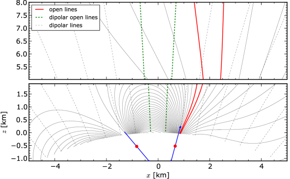
Figure 2.18: Possible non-dipolar structure of the magnetic field lines of PSR B0950+08. The structure was obtained using two crust anchored anomalies located at: ${\bf r_{1}}=\left(0.95R,\,4^{\circ},\,0^{\circ}\right)$, ${\bf r_{2}}=\left(0.95R,\,5^{\circ},\,180^{\circ}\right)$, with the dipole moments ${\bf m_{1}}=\left(5.9\times 10^{-2}d,\,15^{\circ},\,0^{\circ}\right)$, ${\bf m_{2}}=\left(5.9\times 10^{-2}d,\,140^{\circ},\,0^{\circ}\right)$ respectively (blue arrows). The influence of the anomalies is negligible at distances $D\gtrsim 5.0R$, where $B_{{\rm m}}/B_{{\rm d}}\approx m/d=5.9\times 10^{-2}$ (top panel). For more details on the polar cap region see Figure 2.19.

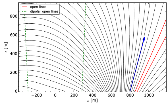
Figure 2.19: Zoom of the polar cap region of PSR B0950+08. See Figure 2.18 for a description.

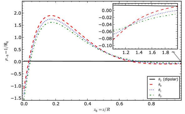
Figure 2.20: Dependence of a curvature of the open magnetic field lines on the distance from the stellar surface for PSR B0950+08. The distance is in units of stellar radius ($z_{6}=z/R$) and the curvature of the magnetic field lines is $\rho_{-6}=1/\Re_{6}=\rho/\left(10^{-6}\,{\rm cm}^{-1}\right)$.

2.4.6 PSR B1133+16

Pulsar B1133+16 is one of the brightest pulsating radio sources in the Northern hemisphere (Maron et al.,, 2000). The relatively long pulse period $P=1.19\,{\rm s}$ and its first derivative $\dot{P}_{-15}\approx 3.5$ result in the following inferred physical properties: $B_{{\rm d}}=4.3\times 10^{12}\,{\rm G}$, $\tau_{c}=5.04\,{\rm Myr}$. The pulsar profile exhibits a classic double peak along with the usual S-shaped polarisation-angle traverse. The pulsar also shows the phenomenon of drifting subpulses but only for some finite time-spans, outside of which the behaviour of individual pulses is chaotic (Honnappa et al.,, 2012).

PSR B1133+16 is located at a high galactic latitude, thus implying a low interstellar extinction (Schlegel et al.,, 1998). Zharikov et al., (2008) suggested a possible optical counterpart with brightness $B=28^{{}^{{\rm mag}}}$.

X-ray observations performed by Kargaltsev et al., (2005) with the Chandra result in a small number of counts ($33$ counts from over $17\,{\rm ks}$), thus the X-ray spectrum can be described by various models. The photon statistics are so low that they allowed only separate fits for the thermal (BB) and nonthermal (PL) components.

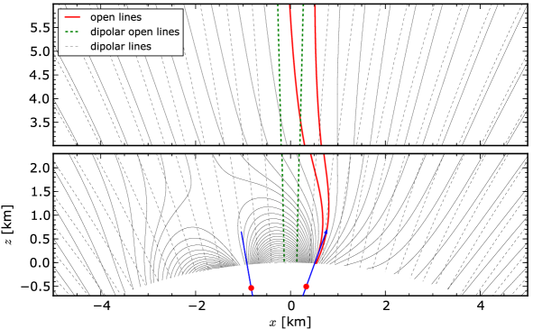
Figure 2.21: Possible non-dipolar structure of the magnetic field lines of PSR B1133+16. The structure was obtained using two crust anchored anomalies located at: ${\bf r_{1}}=\left(0.95R,\,2^{\circ},\,0^{\circ}\right)$, ${\bf r_{2}}=\left(0.95R,\,5^{\circ},\,180^{\circ}\right)$, with the dipole moments ${\bf m_{1}}=\left(8\times 10^{-3}d,\,20^{\circ},\,0^{\circ}\right)$, ${\bf m_{2}}=\left(8\times 10^{-3}d,\,170^{\circ},\,0^{\circ}\right)$ respectively (blue arrows). The influence of the anomalies is negligible at distances $D\gtrsim 4.2R$, where $B_{{\rm m}}/B_{{\rm d}}\approx m/d=5\times 10^{-2}$ (top panel). For more details on the polar cap region see Figure 2.22.

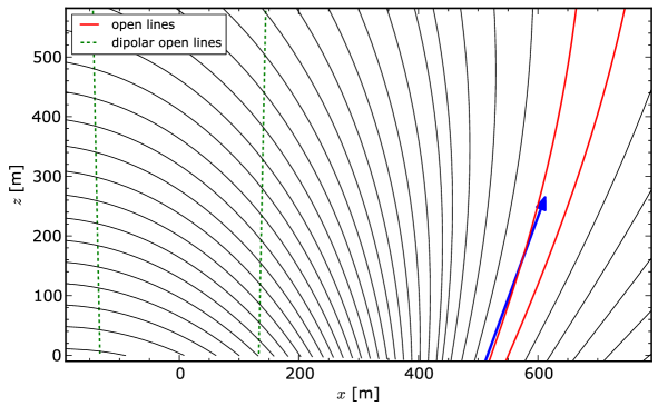
Figure 2.22: Zoom of the polar cap region of PSR B1133+16. See Figure 2.21 for a description.

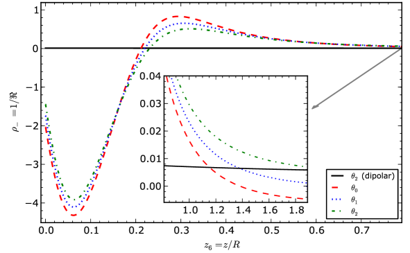
Figure 2.23: Dependence of a curvature of the open magnetic field lines on the distance from the stellar surface for PSR B1133+16. The distance is in units of stellar radius ($z_{6}=z/R$) and the curvature of the magnetic field lines is $\rho_{-6}=1/\Re_{6}=\rho/\left(10^{-6}\,{\rm cm}^{-1}\right)$.

2.4.7 PSR B1929+10

With a pulse period of $P=0.23\,{\rm s}$ and a period derivative of $\dot{P}_{-15}\approx 1.2$, the pulsar’s characteristic age is determined to be $\tau_{c}=3.1\,{\rm Myr}$. These spin parameters imply a dipolar component of the magnetic field at the neutron star magnetic poles $B_{{\rm d}}=1.0\times 10^{12}$. The distance to the pulsar $D=0.36\,{\rm kpc}$ was estimated using the parallax.

Pavlov et al., (1996) identified a candidate optical counterpart of PSR B1929+10 with brightness $U\sim 25.7^{{}^{{\rm mag}}}$, which was later confirmed by proper motion measurements performed by Mignani et al., (2002).

The X-ray pulse profile of PSR B1929+10 consists of a single, broad peak which is in contrast with the sharp radio one of Misanovic et al., (2008). The two-component spectral fit (BB+PL) suggests that both the thermal and nonthermal luminosities are of the same order. The derived surface temperature $T_{{\rm s}}=4.5\,{\rm MK}$ and the surface magnetic field $B_{{\rm s}}=1.3\times 10^{14}\,{\rm G}$ do not coincide with the theoretical curve $T_{{\rm s}}-B_{{\rm s}}$ of the critical temperature calculated by Medin and Lai, (2008). We believe that this inconsistency can be removed by adding an additional blackbody component (the whole surface or the warm spot radiation).

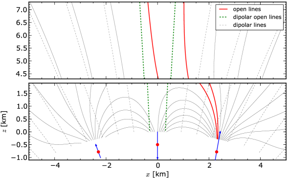
Figure 2.24: Possible non-dipolar structure of the magnetic field lines of PSR B1929+10. The structure was obtained using two crust anchored anomalies located at: ${\bf r_{1}}=\left(0.95R,\,14^{\circ},\,180^{\circ}\right)$, ${\bf r_{2}}=\left(0.95R,\,0^{\circ},\,0^{\circ}\right)$, ${\bf r_{3}}=\left(0.95R,\,14^{\circ},\,0^{\circ}\right)$, with the dipole moments ${\bf m_{1}}=\left(1\times 10^{-2}d,\,20^{\circ},\,180^{\circ}\right)$, ${\bf m_{2}}=\left(2\times 10^{-2}d,\,180^{\circ},\,0^{\circ}\right)$, ${\bf m_{3}}=\left(3\times 10^{-2}d,\,10^{\circ},\,0^{\circ}\right)$ respectively (blue arrows). The influence of the anomalies is negligible at distances $D\gtrsim 4.5R$, where $B_{{\rm m}}/B_{{\rm d}}\approx m/d=3\times 10^{-2}$ (top panel). For more details on the polar cap region see Figure 2.25.

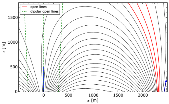
Figure 2.25: Zoom of the polar cap region of PSR B1929+10. See Figure 2.24 for a description.

Figure 2.26: Dependence of a curvature of the open magnetic field lines on the distance from the stellar surface for PSR B1929+10. The distance is in units of stellar radius ($z_{6}=z/R$) and the curvature of the magnetic field lines is $\rho_{-6}=1/\Re_{6}=\rho/\left(10^{-6}\,{\rm cm}^{-1}\right)$.

Chapter 3 Partially Screened Gap

The charge-depleted inner acceleration region above the polar cap can be formed if a local charge density differs from the co-rotational charge density (Goldreich and Julian,, 1969). We assume that the crust of the neutron stars mainly consists of iron $\left({\rm{}_{26}^{56}Fe}\right)$ formed at the neutron star’s birth (e.g. Lai,, 2001). Depending on the mutual orientation of ${\bf\Omega}$ and $\boldsymbol{\mu}$, the stellar surface at the polar caps is either positively (${\bf\Omega}\cdot\boldsymbol{\mu}<0$) or negatively (${\bf\Omega}\cdot\boldsymbol{\mu}>0$) charged. Therefore, the charge depletion above the polar cap depends on the binding energy of either the positive ${\rm{}_{26}^{56}Fe}$ ions or electrons. In this thesis we consider the case of positively charged polar caps (${\bf\Omega}\cdot\boldsymbol{\mu}<0$). We assume that due to the high cohesive energy of iron ions, the positive charges cannot be supplied at a rate that would compensate for the inertial outflow through the light cylinder (see Medin and Lai, (2006, 2007); Gil et al., 2007b ). This is actually possible if the surface temperature $T_{{\rm s}}$ is below the critical value $T_{{\rm crit}}$. Since the number density of the iron ions in the neutron star crust is many orders of magnitude larger than the co-rotational charge density (the so-called Goldreich-Julian density) $\rho_{{\rm GJ}}={\bf\Omega}\cdot{\bf B}/\left(2\pi c\right)$, then a thermionic emission from the polar cap surface is not simply described by the usual condition $\epsilon_{{\rm i}}\approx kT_{{\rm s}}$ , where $\epsilon_{i}$ is the cohesive energy and/or work function, $T_{{\rm s}}$ is the actual surface temperature, and $k$ is the Boltzman constant. The outflow of iron ions can be described in the form (Gil et al., 2003 and references therein)

$$\frac{\rho_{{\rm i}}}{\rho_{{\rm GJ}}}\approx\left(C_{{\rm i}}-\frac{\epsilon_{i}}{kT_{{\rm s}}}\right),$$ (3.1)

where $\rho_{{\rm i}}\leq\rho_{{\rm GJ}}$ is the charge density of the outflowing ions. As soon as the surface temperature $T_{{\rm s}}$ reaches the critical value

$$T_{{\rm crit}}=\frac{\epsilon_{i}}{C_{{\rm i}}k},$$ (3.2)

the ion outflow reaches the maximum value $\rho_{{\rm i}}=\rho_{{\rm GJ}}$. The numerical coefficient $C_{{\rm i}}=30\pm 3$ is determined from the tail of the exponential function with an accuracy of about 10%. Thus, for a given value of the cohesive energy, the critical temperature $T_{{\rm crit}}$ is also estimated within an accuracy of about 10%. The cohesive energy is mainly defined by the strength of the magnetic field and was calculated by Medin and Lai, (2006, 2007).

3.1 The Model

As it follows from the X-ray observations (see Section 1.4), the temperature of the hot spot (which is associated with the actual polar cap) is more than $10^{6}\,{\rm K}$. As we mentioned above, in order to sustain such a high temperature bombardment by the backstreaming particles is required. But particle acceleration (and therefore the surface heating) is possible only if $T_{{\rm s}}<T_{{\rm crit}}$. Gil et al., (2003) introduced the model of the Partially Screened Gap to describe the polar gap sparking discharge specifically under such circumstances.

The PSG model assumes the existence of heavy iron ions (${\rm{}_{26}^{56}Fe}$) with a density near but still below the co-rotational charge density ($\rho_{{\rm GJ}}$), thus the actual charge density causes partial screening of the potential drop just above the polar cap. The degree of screening can be described by screening factor

$$\eta=1-\rho_{{\rm i}}/\rho_{{\rm GJ}}.$$ (3.3)

where $\rho_{{\rm i}}$ is the charge density of the heavy ions in the gap. The thermal ejection of ions from the surface causes partial screening of the acceleration potential drop

$$\Delta V=\eta\Delta V_{{\rm max}},$$ (3.4)

where $\Delta V_{{\rm max}}$ is the potential drop in a vacuum gap. We can express the dependence of the critical temperature on the pulsar parameters by fitting to the numerical calculations of Medin and Lai, (2007)

$$T_{{\rm crit}}=1.6\times 10^{4}\left\{\left[\left(P\dot{P}_{-15}\right)^{0.5}b\right]^{1.1}+17.7\right\},$$ (3.5)

or $T_{{\rm crit}}=1.1\times 10^{6}\left(B_{14}^{1.1}+0.3\right)$, where $B_{14}=B_{{\rm s}}/\left(10^{14}\,{\rm G}\right)$ , $B_{{\rm s}}=bB_{{\rm d}}$ is a surface magnetic field (applicable only if hot spot components are observed, i.e. $b>1$).

The actual potential drop $\Delta V$ should be thermostatically regulated and a quasi-equilibrium state should be established in which heating due to the electron/positron bombardment is balanced by cooling due to thermal radiation (see Gil et al., 2003 for more details). The necessary condition for this quasi-equilibrium state is

$$\sigma T_{{\rm s}}^{4}=\eta e\Delta Vcn_{{\rm GJ}},$$ (3.6)

where $\sigma$ is the Stefan-Boltzmann constant, $e$ - the electron charge, and $n_{{\rm GJ}}=\rho_{{\rm GJ}}/e=1.4\times 10^{11}b\dot{P}_{-15}^{0.5}P^{-0.5}$ is the co-rotational number density. The Goldreich-Julian co-rotational number density can be expressed in terms of $B_{14}$ as

$$n_{{\rm GJ}}=6.93\times 10^{12}B_{14}P^{-1}.$$ (3.7)

Here we assume that the density of backstreaming relativistic electrons is $\eta n_{{\rm GJ}}$.

By using Equations 3.6, 3.5 and 3.7 we can express the acceleration potential drop that satisfies the heating condition (Equation 3.6) as follows

$$\Delta V=7.3\times 10^{5}\frac{\left(B_{14}^{1.1}+0.3\right)^{4}P}{\eta B_{14}}.$$ (3.8)

The above equation may suggest that the acceleration potential drop is inversely proportional to the screening factor. In fact, it is just the opposite (see Equations 3.4 and 3.26).

Knowing that $\Delta V=\gamma_{{\rm max}}mc^{2}/e$, where $m$ is the mass of a particle (electron or positron), we can calculate the maximum Lorentz factor of the primary particles in PSG as

$$\gamma_{{\rm max}}=450\frac{\left(B_{14}^{1.1}+0.3\right)^{4}P}{\eta B_{14}}.$$ (3.9)

3.1.1 Acceleration potential drop

As the actual polar cap is much smaller than the conventional polar cap (see section 1.4.4), we cannot use the approximation proposed by Ruderman and Sutherland, (1975) that the gap height is of the same order as the gap width ($h\approx h_{\perp}$). On the contrary, the small polar cap size and subpulse phenomenon suggest that in the PSG model the spark half-width is considerably smaller than the gap height ($h_{\perp}<h$). For such a regime we need to recalculate a formula for the acceleration potential drop $\Delta V$.

Let us consider a reference frame co-rotating with a star and with the z-axis aligned with the star’s angular velocity ${\bf\Omega}$ (see Figure 3.1).

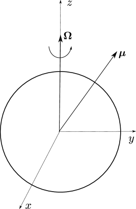
Figure 3.1: Co-rotating frame of reference with the z-axis aligned with the angular velocity ${\bf\Omega}$. The magnetic dipole moment $\boldsymbol{\mu}$ is constant in this frame of reference, thus $\partial{\bf B}/\partial t=0$.

Let us underline that we will neglect the effects of non-inertiality of the co-rotating system. Thus, we assume that in any given moment we have a system moving with a constant velocity.

In this co-rotating frame of reference we can write the spherical components of an angular velocity as follows

$${\bf\Omega}=\left(\Omega\cos\theta,\,-\Omega\sin\theta,\,0\right).$$ (3.10)

Gauss’s law in the co-rotating frame (after Lorentz transformations) takes the form

$$\nabla\cdot{\bf E}=4\pi\rho\left({\bf r}\right)-4\pi\left(\frac{{\bf\Omega}\cdot{\bf B}}{2\pi c}\right).$$ (3.11)

While Faraday’s law of induction can be written as

$$\nabla\times{\bf E}=0.$$ (3.12)

Note that if we consider a drift of plasma in the Inner Acceleration Region (IAR), we should expect temporal variations of the magnetic field ($\nabla\times{\bf E}=-\partial{\bf B}/\left(c\partial t\right)$) (Schiff,, 1939), but as was shown by van Leeuwen and Timokhin, (2012), even if we consider fluctuations of the electric current of the order of the Goldreich-Julian current $\rho_{{\rm GJ}}c$, the resulting variation of the magnetic field is so small that $\nabla\times{\bf E}=0$ with a high accuracy, and circulation of the non-co-rotational electric field along a closed path is zero.

Equation 3.11 in the spherical system of coordinates has the following form

$$\frac{2}{r}E_{r}+\frac{\partial E_{r}}{\partial r}+\frac{\cos\theta}{r\sin\theta}E_{\theta}+\frac{1}{r}\frac{\partial E_{\theta}}{\partial\theta}+\frac{1}{r\sin\theta}\frac{\partial E_{\phi}}{\partial\phi}=4\pi\rho\left(r,\theta,\phi\right)-4\pi\left(\frac{{\bf\Omega}\cdot{\bf B}}{2\pi c}\right).$$ (3.13)

The PSG model assumes the existence of ions in the IAR region that affects the charge density. Using the screening factor, $\eta$, we can write that

$$\rho\left(r,\theta,\phi\right)=\left(1-\eta\right)\rho_{{\rm GJ}}\left(r,\theta,\phi\right)=\left(1-\eta\right)\frac{{\bf\Omega}\cdot{\bf B}}{2\pi c}.$$

In general, $\eta$ depends on the curvature and strength of the magnetic field, thus it varies across the polar cap, but we can still assume that $\eta$ is approximately constant at least for a given spark. Then

$$\frac{2}{r}E_{r}+\frac{\partial E_{r}}{\partial r}+\frac{\cos\theta}{r\sin\theta}E_{\theta}+\frac{1}{r}\frac{\partial E_{\theta}}{\partial\theta}+\frac{1}{r\sin\theta}\frac{\partial E_{\phi}}{\partial\phi}=-4\pi\eta\left(\frac{B_{r}\Omega\cos\theta-B_{\theta}\Omega\sin\theta}{2\pi c}\right).$$ (3.14)

Let us change the variables as follows: $r=R+z$ and $\theta=\alpha+\vartheta$. Here $R$ is the stellar radius and $\alpha$ is the inclination angle between the rotation and the magnetic axis.

$$\frac{2}{R+z}E_{r}+\frac{\partial E_{r}}{\partial z}+\frac{\cos\left(\alpha+\vartheta\right)}{\left(R+z\right)\sin\left(\alpha+\vartheta\right)}E_{\theta}+\frac{1}{R+z}\frac{\partial E_{\theta}}{\partial\vartheta}+\frac{1}{\left(R+z\right)\sin\left(\alpha+\vartheta\right)}\frac{\partial E_{\phi}}{\partial\phi}=\\ =-4\pi\eta\left(\frac{\left(B_{r}\Omega\cos\theta-B_{\theta}\Omega\sin\theta\right)}{2\pi c}\right).$$ (3.15)

Assuming that $R\gg z$, which is correct as the gap height is less than the stellar radius ($h\ll R$), $\alpha\gg\vartheta$, and $B_{r}\gg B_{\theta}$, which is correct for the polar cap region, we can write Equation 3.15 in the first approximation ($R\rightarrow\infty$) as follows

$$\frac{\partial E_{r}}{\partial z}+\frac{1}{R}\frac{\partial E_{\theta}}{\partial\vartheta}=-4\pi\eta\left(\frac{B_{r}\Omega\cos\theta}{2\pi c}\right).$$ (3.16)

Note that for spark widths considerably smaller than the stellar radius $h_{\perp}\ll R$ ($\Delta\vartheta\approx h_{\perp}/R$) we can write that $\frac{1}{R}\frac{\partial E_{\theta}}{\partial\vartheta}\gg\frac{\cot\left(\alpha+\vartheta\right)}{R}E_{\theta}$.

Let us now consider Faraday’s law (Equation 3.12). The curl of an electric field in spherical coordinates can be written as

$$\begin{split}\left({\bf\nabla}\times{\bf E}\right)_{r}=&\frac{1}{r\sin\theta}\left(\frac{\partial}{\partial\theta}\left(E_{\phi}\sin\theta\right)-\frac{\partial E_{\phi}}{\partial\phi}\right)=0,\\ \left({\bf\nabla}\times{\bf E}\right)_{\theta}=&\frac{1}{r}\left(\frac{1}{\sin\theta}\frac{\partial E_{r}}{\partial\phi}-\frac{\partial}{\partial r}\left(rE_{\phi}\right)\right)=0,\\ \left({\bf\nabla}\times{\bf E}\right)_{\phi}=&\frac{1}{r}\left(\frac{\partial}{\partial r}\left(rE_{\theta}\right)-\frac{\partial E{}_{r}}{\partial\theta}\right)=0.\end{split}$$ (3.17)

Using the same change of variables we performed above ($r=R+z$ and $\theta=\alpha+\vartheta$), the third equation of System 3.17 can be written as

$$R\frac{\partial E_{\theta}}{\partial z}=\frac{\partial E_{r}}{\partial\vartheta}.$$ (3.18)

From this equation in the zeroth approximation we can estimate the variations of the electric field components as

$$R\Delta E_{\theta}\Delta\vartheta\approx\Delta E_{r}\Delta z.$$ (3.19)

Since $h_{\perp}\ll R$ we can write that

$$\left\langle h_{\perp}E_{\theta}\right\rangle=\left\langle hE_{r}\right\rangle=\Delta V.$$ (3.20)

From Equation 3.16 we can also briefly estimate that

$$\frac{\Delta E_{r}}{h}+\frac{\Delta E_{\theta}}{h_{\perp}}=-4\pi\eta\left(\frac{B_{r}\Omega\cos\theta}{2\pi c}\right).$$ (3.21)

Using Equations 3.16 and 3.20 we can write that

$$\frac{\left\langle hE_{r}\right\rangle}{h^{2}}+\frac{\left\langle h_{\perp}E_{\theta}\right\rangle}{h_{\perp}^{2}}=\frac{\Delta V}{h^{2}}+\frac{\Delta V}{h_{\perp}^{2}}.$$ (3.22)

Finally, we can estimate the potential drop in a spark region

$$\frac{\Delta V}{h^{2}}+\frac{\Delta V}{h_{\perp}^{2}}=\frac{2\eta B_{r}\Omega\cos\left(\alpha+\vartheta\right)}{c}.$$ (3.23)

If we use the same assumption as Ruderman and Sutherland, (1975), i.e.: (1) the spark half-width is of the same order as the gap height $h_{\perp}=h$, (2) there is no ion extraction from the stellar surface ($\eta=1$), and (3) the pulsar magnetic and rotation axes are aligned ($\alpha=0^{\circ}$), we get:

$$\Delta V_{{\rm RS}}=\frac{B_{r}\Omega}{c}h^{2}.$$ (3.24)

Note that the potential drop defined by Equation 3.23 differs from that used in the Standard Model by the screening factor (as the presence of ions screens the gap) and by the factor of $\cos\left(\alpha+\vartheta\right)$ which also takes into account non-aligned pulsars. In our case the polar cap size is much smaller than the conventional polar cap size. It seems reasonable to also consider sparks with widths much smaller than the gap height ($h_{\perp}\ll h$), in that case the potential drop can be calculated as

$$\Delta V=\frac{2\eta B_{r}\Omega\cos\left(\alpha+\vartheta\right)}{c}h_{\perp}^{2}.$$ (3.25)

Even for a relatively small inclination angle between the rotation and magnetic axis, we can still write $\vartheta\ll\alpha$, thus

$$\Delta V=\frac{4\pi\eta B_{r}\cos\alpha}{cP}h_{\perp}^{2}.$$ (3.26)

3.1.2 Acceleration path

Since the exact dependence of the electric field on $z$ is unknown we use the same linear approximation that Ruderman and Sutherland, (1975) used. In the frame of the PSG model as $h_{\perp}<h$ or even $h_{\perp}\ll h$, we can use Equations 3.20 and 3.26 to describe the component of the electric field along the magnetic field line:

$$E\approx\frac{8\pi\eta B_{{\rm s}}\cos\alpha}{cP}\frac{h_{\perp}^{2}}{h^{2}}\left(h-z\right),$$ (3.27)

which vanishes at the top $z=h$. The Lorentz factor of particles after passing distance $l_{{\rm acc}}$ can be calculated as follows

$$\gamma_{{\rm acc}}=\frac{e}{mc^{2}}\int_{z_{1}}^{z_{2}}Edz\approx\frac{8\pi\eta B_{{\rm s}}e\cos\alpha}{mc^{3}P}\frac{h_{\perp}^{2}}{h^{2}}\left(z_{2}-z_{1}\right)\left(h-\frac{z_{1}+z_{2}}{2}\right),$$ (3.28)

where $m$ is the mass of a particle (electron or positron) and $z_{2}-z_{1}=l_{{\rm acc}}$. Then we can approximate $z_{1}+z_{2}\approx h$, thus

$$l_{{\rm acc,ap}}=\frac{\gamma_{{\rm acc}}mc^{3}P}{4\pi\eta B_{{\rm s}}e\cos\alpha}\frac{h}{h_{\perp}^{2}}.$$ (3.29)

Assuming that a non-relativistic particle is accelerated from the stellar surface ($z_{1}=0$, $\gamma_{0}=1$) we can calculate the distance $l_{{\rm acc}}$ which it should pass to gain a Lorentz factor $\gamma_{{\rm acc}}$:

$$l_{{\rm acc}}=h\left(1-\sqrt{1-\frac{2\gamma}{\ell}}\right),$$ (3.30)

where $\ell=8\pi\eta B_{{\rm s}}eh_{\perp}^{2}\cos\left(\alpha\right)/\left(Pc^{3}m\right)$. Although the approximate formula 3.29 is much more readable, in the calculations we use the exact value (see Equation 3.30) as for Lorentz factors that are considerably smaller than the maximum value, the discrepancy is about a factor of two, $l_{{\rm acc,ap}}\approx 2l_{{\rm acc}}$.

3.1.3 Electron/positron mean free path

The mean free path of a particle (electron and/or positron) $l_{{\rm p}}$ can be defined as the mean length that a particle passes until a $\gamma$-photon is emitted. In the case of the CR particle, mean free path can be estimated as a distance that a particle with a Lorentz factor $\gamma$ travels during the time which is necessary to emit a curvature photon (see Zhang et al., 1997)

$$l_{{\rm CR}}\sim c\left(\frac{P_{{\rm CR}}}{E_{\gamma,{\rm CR}}}\right)^{-1}=\frac{9}{4}\frac{\hbar\Re c}{\gamma e^{2}},$$ (3.31)

where $P_{{\rm CR}}=2\gamma^{4}e^{2}c/3\Re^{2}$ is the power of CR, $E_{\gamma,{\rm CR}}=3\hbar\gamma^{3}c/2\Re$ is the photon characteristic energy, and $\Re$ is the curvature radius of the magnetic field lines.

For the ICS process calculation of the particle mean free path $l_{{\rm ICS}}$ is not as simple as that of the CR process. Although we can define $l_{{\rm ICS}}$ in the same way that we defined $l_{{\rm CR}}$, it is difficult to estimate the characteristic frequency of emitted photons. We have to take into account photons of various frequencies with various incident angles. An estimation of the mean free path of an electron (or positron) to produce a photon is in Xia et al., (1985)

$$l_{{\rm ICS}}\sim\left[\int_{\mu_{0}}^{\mu_{1}}\int_{0}^{\infty}\sigma^{\prime}\left(\epsilon,\mu\right)\left(1-\beta\mu_{i}\right)n_{{\rm ph}}\left(\epsilon\right)d\epsilon d\mu\right]^{-1}.$$ (3.32)

Here $\epsilon$ is the incident photon energy in units of $mc^{2}$, $\mu=\cos\psi$ is the cosine of the photon incident angle, $\beta=v/c$ is the velocity in terms of speed of light, $\sigma^{\prime}$ is the cross section of ICS in the particle rest frame,

$$n_{{\rm ph}}\left(\epsilon,\,T\right)d\epsilon=\frac{4\pi}{\lambda_{c}^{3}}\frac{\epsilon^{2}}{\exp\left(\epsilon/\mho\right)-1}d\epsilon$$ (3.33)

represents the photon number density distribution of semi-isotropic blackbody radiation, $\mho=kT/mc^{2}$, $k$ is the Boltzmann constant, and $\lambda_{c}=h/mc=2.424\times 10^{-10}$ cm is the electron Compton wavelength. A detailed description of how to calculate $\sigma^{\prime}$ can be found in Section 4.4.1.

We should expect two modes of ICS: resonant and thermal-peak (see Section 4.4.3 for more details). The Resonant ICS (RICS) takes place if the photon frequency in the particle rest frame is equal to the electron cyclotron frequency. As shown in Section 4.4.4, the particle mean free path strongly depends on the distance from the polar cap. Both the photon density and incident angles ($\mu_{0}$ and $\mu_{1}$) change with increasing altitude. In our calculations we take into account both of those effects, thus we replace $n_{{\rm ph}}\left(\epsilon,\,T\right)$, $\mu_{0}$ and $\mu_{1}$ with $n_{{\rm sp}}\left(\epsilon,\,T,\,L\right)$, $\mu_{{\rm min}}$$\left(L\right)$ and $\mu_{{\rm max}}\left(L\right)$, respectively (for more details see Section 4.4.4). Here, $L$ is the location of the particle, $n_{{\rm sp}}\left(\epsilon,\,T,\,L\right)$ is the photon density at location $L$, and $\mu_{{\rm min}}\left(L\right)$ and $\mu_{{\rm max}}$$\left(L\right)$ correspond to the highest and lowest angle between the photons and particle at a given location $L$. Thus, just above the polar cap for RICS the mean free path of outflowing positrons is:

$$l_{{\rm RICS}}\approx\left[\int_{\mu_{{\rm min}}\left(L\right)}^{\mu_{{\rm max}}\left(L\right)}\int_{\epsilon_{{}_{{\rm res}}}^{{\rm{}^{min}}}}^{\epsilon_{{}_{{\rm res}}}^{{\rm{}^{max}}}}\left(1-\beta\mu\right)\sigma^{\prime}\left(\epsilon,\mu\right)n_{{\rm sp}}\left(\epsilon,\,T,\,L\right)d\epsilon d\mu\right]^{-1},$$ (3.34)

where the limits of integration over energy, $\epsilon_{{\rm{}_{res}}}^{{\rm{}^{min}}}$ and $\epsilon_{{\rm{}_{res}}}^{{}^{{\rm max}}}$, are chosen to cover the resonant energy (for more details see Section 4.4.3).

The thermal-peak ICS (TICS) includes all scattering processes of photons with frequencies around the maximum of the thermal spectrum. As an example we adopt $\epsilon_{{}_{{\rm th}}}^{{\rm{}^{min}}}\approx 0.05\epsilon_{{\rm{}_{th}}}$, and $\epsilon_{{}_{{\rm th}}}^{{\rm{}^{{\rm max}}}}\approx 2\epsilon_{{}_{{\rm th}}}$ where $\epsilon_{{}_{{\rm th}}}=2.82kT/\left(mc^{2}\right)$ is the energy, in units of $mc^{2}$, at which blackbody radiation with temperature $T$ has the largest photon number density. The electron/positron mean free path for the TICS process is

$$l_{{\rm TICS}}\approx\left[\int_{\mu_{{\rm min}}\left(L\right)}^{\mu_{{\rm max}}\left(L\right)}\int_{\epsilon_{{}_{{\rm th}}}^{{\rm{}^{min}}}}^{\epsilon_{{}_{{\rm th}}}^{{\rm{\rm{}^{max}}}}}\left(1-\beta\mu\right)\sigma^{\prime}\left(\epsilon,\mu\right)n_{{\rm ph}}\left(\epsilon,\,T,\,L\right)d\epsilon d\mu\right]^{-1}.$$ (3.35)

3.1.4 Photon mean free path

The photons with energy $E_{\gamma}>2mc^{2}$ propagating obliquely to the magnetic field lines can be absorbed by the field, and as a result, an electron-positron pair is created. To describe the strength of the magnetic field we use $\beta_{q}=B/B_{q}$, where $B_{q}=m^{2}c^{3}/e\hbar=4.413\times 10^{13}\,{\rm G}$ is the critical magnetic field strength.

For strong magnetic fields ($\beta_{q}\gtrsim 0.2$, see Section 4.2.3) the photon mean free path can be calculated as (see Section 4.2.4 for more details)

$$l_{{\rm ph}}\approx\Re\frac{2mc^{2}}{E_{\gamma}},$$ (3.36)

while for weaker magnetic fields ($\beta_{q}\lesssim 0.2$) we can use an asymptotic approximation derived by Erber, (1966)

$$l_{{\rm ph}}=\frac{4.4}{(e^{2}/\hbar c)}\frac{\hbar}{mc}\frac{B_{q}}{B\sin\Psi}\exp\left(\frac{4}{3\chi}\right),$$ (3.37)

$$\chi\equiv\frac{E_{\gamma}}{2mc^{2}}\frac{B\sin\Psi}{B_{q}}\hskip 28.45274pt(\chi\ll 1),$$ (3.38)

where $\Psi$ is the angle of intersection between the photon and the local magnetic field.

3.2 Gap height

By knowing the acceleration potential drop in PSG $\Delta V$ we can evaluate the gap height $h$ and the screening factor $\eta$, which actually depends on the details of the avalanche pair production in the gap. First, we need to determine which process, Curvature Radiation (CR) or Inverse Compton Scattering (ICS), is responsible for the $\gamma$-photon generation in the gap region. In order to identify the proper process we need the following parameters: $l_{{\rm acc}}$ - the distance which a particle should pass to gain the Lorentz factor $\gamma_{{\rm acc}}$, $l_{{\rm p}}$ - the mean length a particle (electron and/or positron) travels before a $\gamma$-photon is emitted, and $l_{{\rm ph}}$ - the mean free path of the $\gamma$-photon before being absorbed by the magnetic field.

As mentioned above, PSG can exist if Equation 3.6 is satisfied. On the other hand, in order to heat the polar cap surface to high enough temperatures the high enough flux of back-streaming particles is required. By using Equations 3.8 and 3.26 we can find the relationship between the screening factor, the spark half-width and pulsar parameters

$$\eta h_{\perp}=4.17\frac{\left(B_{14}^{1.1}+0.3\right)^{2}P}{B_{14}\sqrt{\left|\cos\alpha\right|}}.$$ (3.39)

Thus, for specific pulsar parameters we can define a product of the two main parameters of PSG, namely the screening factor $\eta$ and the spark half-width $h_{\perp}$.

3.2.1 Particle mean free paths, CR vs. ICS gap

The Figure 3.2 shows the dependence of particle mean free paths on the Lorentz factor $\gamma$ for some pulsar parameters (the dependence on pulsar parameters will be discussed in Section 3.3). Let us note that these free paths do not depend on the gap height $h$ (see Equations 3.31, 3.32 and 3.36). The results presented in the Figure do not allow to define the gap height unambiguously. However, we can find which process is responsible for generation of the $\gamma$-photon in PSG. For narrow sparks the acceleration potential drop decreases, and as a result the Lorentz factor of the primary particles is about $\gamma\sim 10^{3}-10^{4}$. In this regime $l_{{\rm ICS}}\ll l_{{\rm CR}}$, so the gap will be dominated by ICS. Thus, ICS will dominate the gap if deceleration due to Inverse Compton Scattering prevents further acceleration by the electric field. Let us remember that ICS is not efficient for particles with the Lorentz factor $\gamma\gtrsim 10^{5}$. If the sparks are wider or $\eta\approx 1$, the acceleration potential drop increases and the Lorentz factors of primary particles reach values about $\gamma\sim 10^{5}-10^{6}$. In this regime the $\gamma$-photon emission is dominated by CR. Let us note that the condition $l_{{\rm ICS}}\ll l_{{\rm CR}}$ is satisfied for particles with $\gamma\sim 10^{3}-10^{4}$, as one can see from Figure 3.2 (panel a), but this does not mean that the ICS event happens. Since $l_{{\rm acc}}\ll l_{{\rm ICS}}$, the particles will be accelerated to higher energies ($\gamma\sim 10^{5}-10^{6}$) before they upscatter the X-ray photons. Thus, the particles start emission of $\gamma$-photons (via CR) as soon as condition $l_{{\rm acc}}\approx l_{{\rm CR}}$ is met.

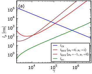
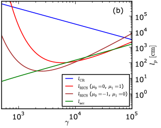
Figure 3.2: Dependence of the mean free path of the primary particle on Lorentz factor $\gamma$ for both the CR and ICS processes. Panel (a) corresponds to calculations for a relatively higher potential drop (e.g. a wider spark with $h_{\perp}=3\,{\rm m}$ and $\eta=1$), while panel (b) corresponds to calculations for a relatively lower potential drop (e.g. a narrow spark with $h_{\perp}=1\,{\rm m}$ and $\eta=0.1$). The acceleration paths on both panels were calculated for the same pulsar parameters ($B_{14}=3.5$, $T_{6}=4.4$, $\Re_{6}=1$, $P=1$, $\alpha=10^{\circ}$). Note that for the RICS process the particle mean free paths were calculated for optimal conditions (just above the polar cap).

3.2.2 Possible scenarios of the gap breakdown: PSG-on and PSG-off modes

As is seen from Figures 3.3 and 3.4, in the CR-dominated gap the primary particle should travel a distance comparable with gap height $l_{{\rm acc}}\approx h/2$ in order to gain an energy corresponding to the characteristic Lorentz factor $\gamma_{{\rm c}}^{{\rm{}^{CR}}}$. On the other hand, the primary particles in the ICS-dominated gap reach a characteristic value $\gamma_{{\rm c}}^{{\rm{}^{ICS}}}$ at altitudes that are considerably smaller than gap height $l_{{\rm acc}}\ll h$ (see Figures 3.3 and 3.5). Thus, $\gamma_{{\rm c}}^{{\rm{}^{CR}}}\approx 10^{6}\approx\gamma_{{\rm max}}$ is about three orders of magnitude higher than $\gamma_{{\rm c}}^{{}^{{\rm ICS}}}\approx 10^{3}\ll\gamma_{{\rm max}}$, here $\gamma_{{\rm max}}$ is the value of the Lorentz factor after the particle travels a distance $h$. Furthermore, the characteristic energy of CR photons is considerably smaller than the energy of emitting (primary) particles, e.g. for $\gamma=10^{6}$, $\Re_{6}=1$, $\gamma_{{\rm sec}}\approx 10^{2}$. On the other hand, RICS photons upscattered in an ultrastrong ($B>B_{{\rm crit}}$) magnetic field gain a significant part of the energy of the scattering (primary) particle. Therefore, the electron/positron pair created by the RICS photon has energies comparable with the energy of the scattering (primary) particle. This will essentially influence the multiplicity $M_{{\rm pr}}$ in the ICS gap, as all the newly created particles will participate in further cascade pair-production. Additionally, RICS in ultrastrong magnetic fields produces approximately the same amount of photons with $\parallel$ and $\perp$ polarisation (see Section 4.4.2), while most of the photons produced by CR are $\parallel$-polarised (see Section 4.1). Splitting of the $\perp$-polarised photons will increase the photon mean free path, but it will also increase the multiplicity in the ICS gaps.

Figure 3.3 presents a sketch of a cascade formation for CR- and ICS-dominated gaps. The CR photons are emitted in the upper half of the gap. Most of these photons produce pairs at about the same height, in the region where the acceleration potential is almost equal to zero, hereinafter we will call this region the Zero-Potential Front (ZPF). The newly created particles have much lower Lorentz factors as compared with the primary particle, thus they are not able to emit CR photons.

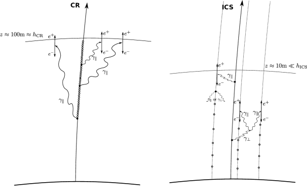
Figure 3.3: Sketch of differences in a cascade formation for the CR-dominated gap (left panel) and the ICS-dominated gap (right panel). In order to increase readability, only a few points (filled circles) are shown which correspond to altitudes where $\gamma$-photons are emitted. The unfilled circles correspond to places where $\gamma$-photons are also emitted, but those photons (and their evolution) are not included in the diagram. Note that for the ICS-dominated gap we plot only the bottom (active) part of the gap ($z\ll h_{{\rm ICS}}$), furthermore, points of radiation are tracked only for the first population of newly created particles. The avalanche nature of the ICS-dominated gap will result in a much higher multiplicity and continuous backflow of relativistic particles.

Figure 3.4 presents the primary particle evolution and photon mean free paths of $\gamma$-rays produced in the CR-dominated gap. As can be seen, the first $\gamma$-photon produces a pair approximately at the same time (and same place) as the primary particle reaches ZPF. Thus, the multiplicity in a gap region (the number of particles created by a single primary particle) in the CR scenario is strictly related to the number of photons produced by the primary particle $M_{{\rm CR}}\approx 2\times N_{{\rm ph}}^{{\rm{}^{CR}}}$.

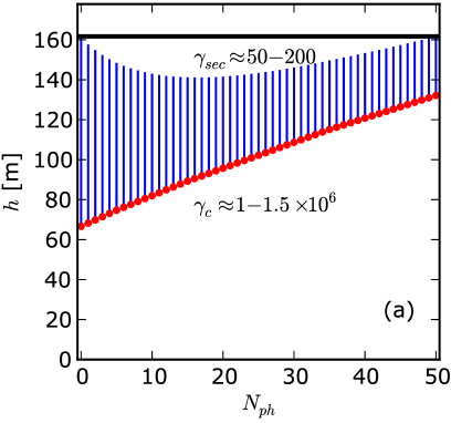
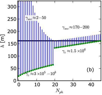
Figure 3.4: Cascade formation for a CR-dominated gap. Blue lines represent the mean free path of $\gamma$-photons. The filled circles correspond to places of $\gamma$-photon emission. Panel (a) includes the free paths of $\gamma$-photons which produce pairs below ZPF (red circles) while panel (b) includes the free paths of $\gamma$-photons which produce pairs above the acceleration gap (blue circles). The results were obtained using the following parameters: $N_{{\rm ph}}^{{}^{{\rm CR}}}=50$, $B_{{\rm s}}=2.3\times 10^{14}\,{\rm G}$, $B_{{\rm d}}=2.9\times 10^{14}\,{\rm G}$, $T=3\,{\rm MK}$, $P=1.3\,{\rm s}$, $\Re_{6}=0.5$, and $\alpha=60.7^{\circ}$.

The energy of $\gamma$-photons produced by ICS depends on the Lorentz factor of the primary particles and on the strength of the magnetic field. In ultrastrong magnetic fields the energy of newly created particles is comparable with the energy of the scattering particle $\gamma_{{\rm new}}\approx\gamma_{{\rm c}}/2$. Figure 3.5 shows schematically the locations at which $\gamma$-photons are emitted by ICS. The first $\gamma$-photon is produced already at altitudes of about a few metres and then converted to an electron-positron pair well below ZPF. Note that already at relatively low altitudes ($z\gtrsim 100\,{\rm m}$) the photon density decreases rapidly (see Section 4.4.4.1), furthermore, the small size of the polar cap entails a rapid change of the particle-photon incident angles (see Section 4.4.4.2). Those two effects make the ICS process significant only in the lower parts of the gap ($z\lesssim 20\,{\rm m}$). On the other hand, the multiplicity in the ICS-dominated gap is enhanced by all newly created particles which are created in the lower part of the gap. Furthermore, the ICS is more effective for backstreaming particles (see Figure 3.2), thus most of the $\gamma$-photons in the gap region will be created by scatterings on electrons. For the ICS scenario it is not possible to evaluate a simple expression for the multiplicity produced by a single primary particle in a gap region. Furthermore, it is not possible to determine the actual value of $N_{{\rm ph}}$ required to break the gap (both for CR and ICS) without a full cascade simulation.

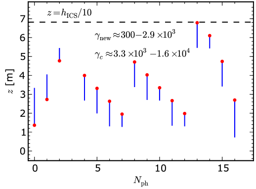
Figure 3.5: Cascade formation for an ICS-dominated gap. Blue lines represent the mean free path of $\gamma$-photons. The filled circles correspond to places of $\gamma$-photon emission. The results were obtained using the following parameters: $N_{{\rm ph}}^{{}^{{\rm ICS}}}=15$, $B_{{\rm s}}=2.3\times 10^{14}\,{\rm G}$, $B_{{\rm d}}=2.9\times 10^{14}\,{\rm G}$, $T_{{\rm s}}=3\,{\rm MK}$, $P=1.3\,{\rm s}$, $\Re_{6}=0.5$, and $\alpha=60.7^{\circ}$.

The differences between the CR and ICS gaps that we mention above have drastic consequences on the cascade formation process. Since the cooling time of the hot spot is very short ($\tau_{{\rm cool}}\lesssim 10^{-8}\,{\rm s}$ , see Gil et al.,, 2003), to sustain the hot spot temperature just below the critical temperature a continuous backflow of relativistic particles is required. An energetic enough flux of backstreaming particles can be produced only in ICS-dominated gaps. The heating of the surface will sustain the outflow of iron ions from the crust, maintaining $\eta<1$, hence we call this mode the PSG-on mode. As the temperature of the polar cap is in quasi equilibrium with the backstreaming particles (temperature is close to the critical value) the gap can break only due to production of a dense enough plasma $n_{p}\gg\eta n_{{\rm GJ}}$ in the gap region. The multiplicity in the PSG-on mode is much higher than the multiplicity of CR-dominated gaps. Moreover, in the gap dominated by CR the particles are created in a cloud-like fashion (see Figure 3.4). The successive clouds heat up the surface once per $\tau_{{\rm 0}}\approx 2h/c$, which for a typical gap height $h\approx 100\,{\rm m}$ is much longer than the time needed for the surface to cool down $\tau_{{\rm 0}}\approx 6\times 10^{-7}\gg\tau_{{\rm cool}}$. Therefore, in the CR-dominated gaps the backstreaming particles cannot sustain the temperature that is close to the critical value during $\tau_{{\rm 1}}\gg\tau_{0}\gg\tau_{{\rm cool}}$, thus for most of the time the screening factor is $\eta\approx 1$ and we call this mode the PSG-off mode. The low multiplicity of a cascade in the PSG-off mode can cause that the gap to breakdown only due to overheating of the surface, but not due to production of a dense enough plasma. The growth of particle density will continue to the point when the backstreaming particles heat up the surface to a temperature equal to or higher than the critical temperature, $\tau_{{\rm heat}}\gg\tau_{0}$. Let us note that the primary particles in the PSG-off mode are very energetic $\gamma\approx 10^{6}$, and hence the density of particles required to close gap $\rho_{c}$ is much lower than the Goldreich-Julian density. To describe this difference we use the overheating parameter $\kappa=\rho_{c}/\rho_{{\rm GJ}}$. Knowing that in the PSG-off mode $\eta\approx 1$, we use Equation 3.6 and the relation $\Delta V=\gamma_{{\rm acc}}mc^{2}/e$ to calculate the overheating parameter:

$$\kappa=\frac{\sigma\,T^{4}}{n_{{\rm GJ}}\,\gamma_{{\rm max}}\,mc^{3}}.$$ (3.40)

3.2.3 PSG-off mode

Curvature emission by a primary particle is effective for Lorentz factors $\gamma\gtrsim 10^{5}$ (when $l_{{\rm CR}}\leq l_{{\rm acc}}$). An equilibrium between acceleration and deceleration (by reaction force) would be established if the CR power were equal to the ”electric power”. In our case ($\Re_{6}\approx 1$, $\gamma_{{\rm c}}\approx 10^{6}$), the reaction force is not high enough to stop acceleration by the electric field. In the PSG-off mode the spark region is free from ions ($\eta\approx 1$), thus the heating condition (Equations 3.6 and 3.39) is no longer satisfied. Taking into account the curvature of magnetic field lines just above the stellar surface, we can estimate the dependence of the minimum spark half-width on the gap height (see Figure 3.6):

$$h_{\perp}^{{\rm{}^{min}}}=\Re-\sqrt{\Re^{2}-h^{2}}.$$ (3.41)

Figure 3.7 presents the minimum spark half-width for three different radii of curvature: $\Re_{6}=0.1$, $\Re_{6}=0.5$, $\Re_{6}=1$. Note that as long as the gap height does not exceed some specific value ($h\approx 40\,{\rm m}$, $h\approx 100\,{\rm m}$, $h\approx 140\,{\rm m}$, respectively for the given curvature radii) the minimum spark half-width is well below $1\,{\rm m}$.

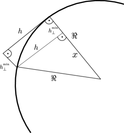
Figure 3.6: Diagram of the minimum spark half-width $h_{\perp}^{{\rm{}^{min}}}$ for a given gap height $h$ and a radius of curvature $\Re$.

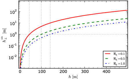
Figure 3.7: Minimum spark half-width vs. gap height calculated for three different radii of curvature: $\Re_{6}=0.1$ - red solid line, $\Re_{6}=0.5$ - green dashed line, and $\Re_{6}=1$ - blue dotted line.

On the other hand, we can estimate the acceleration potential $\Delta V$ (and thus the spark half-width $h_{\perp}^{{}^{{\rm N_{{\rm ph}}}}}$) required to produce a specified number of photons $N_{{\rm ph}}^{{}^{{\rm CR}}}$ within a gap. Figure 3.8 presents the dependence of both $h_{\perp}^{{}^{{\rm min}}}$ and $h_{\perp}^{{\rm{}^{N_{{\rm ph}}}}}$ on the gap height. As results from the Figure, the gap height in PSG-off does not change drastically with $N_{{\rm ph}}^{{}^{{\rm CR}}}$, and for these specific parameters of a pulsar it is $h\approx 240\,{\rm m}$. For historical reasons, hereafter unless stated otherwise, we will use $N_{{\rm ph}}^{{}^{{\rm CR}}}=50$ to calculate the gap parameters of the PSG-off mode. Note that in order to find the gap height, we assume $h_{\perp}^{{}^{{\rm min}}}=h_{\perp}^{{}^{N_{{\rm ph}}}}$, which results in a gap that allows both overheating of the entire spark surface by backstreaming particles and the creation of the required number of photons $N_{{\rm ph}}^{{}^{{\rm CR}}}$.

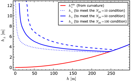
Figure 3.8: Dependence of a spark half-width on the gap height for the PSG-off mode. The results were obtained using the following pulsar parameters: $B_{14}=2.3$, $T_{6}=3.0$, $P=1.3\,{\rm s}$, $\Re_{6}=1.0$, $\alpha=60.7^{\circ}$.

In our calculations we use the algorithm presented in Figure 3.9 to find the gap height in the PSG-off mode for given pulsar parameters: a pulsar period $P$, a pulsar inclination angle $\alpha$, a surface magnetic field strength $B_{{\rm s}}$, and a curvature radius of field lines $\Re$.

Figure 3.9: Flowchart of the algorithm used to estimate the gap height in the PSG-off mode. The initial gap height from which we begin our calculations is an arbitrary set to $h_{{\rm init.}}=10\,{\rm m}$, while the step $\Delta h$ depends on the required accuracy. The number of $\gamma$-ray photons created in a spark by a single primary particle is set to $N_{{\rm ph}}^{{\rm{}^{CR}}}=50$ (see text for more details).

Figure 3.10 presents the result of finding the gap height in the PSG-off mode for PSR B0943+10. The presented solution corresponds to the magnetic field structure presented in Section 2.4.4. The average radius of curvature in the gap region is relatively high, $\Re_{6}=0.7$, hence the inclination of the gap region. The polar gap conditions, the strength of magnetic field $B_{14}=2.4$ ($R_{{\rm bb}}=17\,{\rm m}$) and the polar cap temperature $T_{6}=3.0$ were restrained to follow the observed values (see Table 1.4). The presented solution corresponds to the following PSG parameters: gap height $h=166\,{\rm m}$, spark half-width $h_{\perp}=1.9\,{\rm m}$, $\eta=1$ (fixed), $\kappa=7\times 10^{-3}$, $\gamma_{{\rm c}}=1.4\times 10^{6}$. Note that the primary particles will gain $\gamma_{{\rm max}}=1.9\times 10^{6}$ as the CR efficiency is not high enough to stop the acceleration.

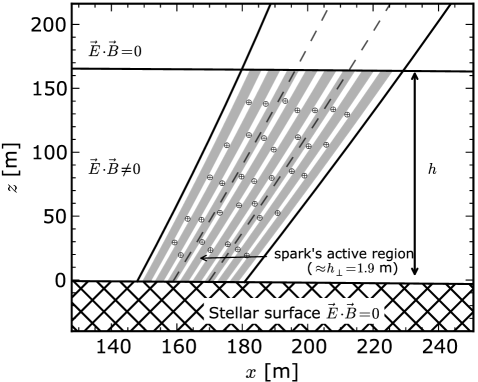
Figure 3.10: Gap structure in the PSG-off mode for PSR B0943+10. Filled columns represent the locations and sizes of the active regions of sparks. Here we assumed that the active region of a spark (the place where acceleration is high enough to produce a cascade) has a size comparable with the spark half-width. The iron ions extracted from the surface (due to a high surface temperature) are represented by circle-plus symbols.

3.2.4 PSG-on mode

In the PSG-on mode, radiation of the surface just below the spark is in quasi-equilibrium with the flux of backstreaming particles. When the surface temperature rises, the density of iron ions increases, thus resulting in a decrease in the potential drop, which in turn, reduces the flux of backstreaming particles. On the other hand, when the surface temperature decreases it entails the drop of iron ion density and, consequently, an increase in the flux of backstreaming particles. Thus the polar cap temperature is maintained slightly below the critical value. This quasi-equilibrium state prevents the gap breakdown due to surface overheating. However, a high multiplicity in the PSG-on mode leads to a production of dense plasma. When the density of the plasma $n_{p}\gg\eta n_{{\rm GJ}}$, the acceleration potential drop will be completely screened due to charge separation.

Alongside the pulsar parameters the gap height in the PSG-on mode also depends on the spark half-width $h_{\perp}$ and on the number of scatterings by the first population of newly created particles $N_{{\rm ph}}^{{\rm{}^{ICS}}}$. For a sample of pulsars we can use drift information to put constraints on the spark half-width (see Section 3.4). Figure 3.11 presents the procedure of finding the gap height in the PSG-on mode for the following pulsar parameters: a pulsar period $P$, a pulsar inclination angle $\alpha$, a surface magnetic field strength $B_{{\rm s}}$, a surface temperature $T_{{\rm s}}$, a curvature radius of magnetic field lines $\Re$, and a spark half-width $h_{\perp}$. First we use Equation 3.6 to estimate the screening factor $\eta$ which defines the electric field, and thus the particle acceleration. Then we estimate the number of scatterings for a single outflowing particle $N_{{\rm ph}}^{{\rm{}^{pr}}}$ for the initial gap height. The initial gap height from which we begin our calculations is an arbitrary set to $h_{{\rm init.}}=10\,{\rm m}$. We track the propagation of $\gamma$-photons produced by ICS on a primary particle to find the location $L_{{\rm new}}$ where pairs are created. Then we calculate their propagation through the acceleration region and we estimate the number of scatterings by every newly created particle of the first population $N_{{\rm ph}}^{{\rm{}^{new}}}$. If the total number of scatterings by the first population (including the primary particle) is $N_{{\rm ph}}<N_{{\rm ph}}^{{\rm{}^{ICS}}}$ , we resume our calculations assuming a higher gap until the $N_{{\rm ph}}\geq N_{{\rm ph}}^{{\rm{}^{ICS}}}$ is met.

Figure 3.11: Flowchart of algorithm used to estimate the gap height in PSG-on mode for a given spark half-width (see text for more details).

As a result we obtain the gap parameters: the gap height $h$, the screening factor $\eta$, the characteristic Lorentz factor of a particle at the moment of ICS photon emission $\gamma_{{\rm c}}$, the maximum value of the Lorentz factor $\gamma_{{\rm max}}$, and the characteristic Lorentz factor of iron ions $\gamma_{{\rm i}}$. In our calculations, if not stated otherwise, we use $N_{{\rm ph}}^{{}^{{\rm ICS}}}=25$ to calculate the gap parameters of the PSG-on mode. Note that in this approximation we take into account only the first population of newly created particles. In fact, the avalanche nature of the ICS-dominated gap will result in a much higher multiplicity than in the PSG-off mode $M_{{\rm ICS}}\gg M_{{\rm CR}}$. For details of particle/photon propagation, see Chapter 4. Subpulse drift observations are available only for a few X-ray pulsars with the hot spot component. Thus, to find the approximate gap parameters for pulsars without the predicted spark half-width we use $h_{\perp}=2\,{\rm{\rm m}}$.

Figure 3.12 presents the result of finding the gap height in the PSG-on mode for PSR B0943+10. In this model the gap parameters, such as the magnetic field strength $B_{{\rm s}}$ and the surface temperature $T_{{\rm s}}$, were restrained to follow the observed values (see Table 1.4). The result was obtained for the non-dipolar structure of a surface magnetic field presented in Section 2.4.4 and for the predicted value of a spark half-width $h_{\perp}\approx 2\,{\rm m}$ (see Table 3.3). The height required to produce $N_{{\rm ph}}^{{\rm{}^{ICS}}}=25$ photons by the first population of particles was estimated as $h\approx 92\,{\rm m}$. Other gap parameters for this solution can be found in Table 3.1.

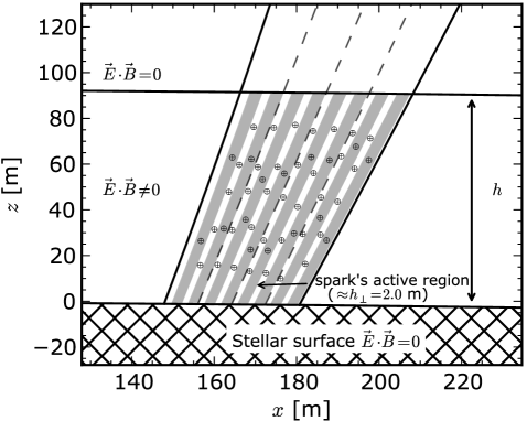
Figure 3.12: Gap structure in the PSG-on mode for PSR B0943+10. Filled columns represent the locations and sizes of the active regions of sparks. Here we assumed that the active region of a spark (the place where acceleration is high enough to produce a cascade) has a size comparable with the spark half-width. The iron ions extracted from the surface (due to a high surface temperature) are represented by circle-plus symbols. Note that iron ions are present in both the non-active and active regions. The density of ions in the non-active regions is so high that it prevents cascade formation of pairs.

3.2.5 Results

In Table 3.1 we present the results of finding the gap height for the sample of pulsars. For the PSG-on mode we show the estimated PSG parameters found using the predicted spark half-width and the spark half-width $h_{\perp}=2\,{\rm m}$. The only exception is Geminga (PSR J0633+1746), for which drift information is not available and we can only present calculations for $h_{\perp}=2\,{\rm m}$. For PSR B0628-28 the predicted spark half-width is large ($h_{\perp}=3.9\,{\rm m}$), which entails a high acceleration potential. For such wide sparks it is not possible to find the PSG-on solution with the required number of scatterings $N_{{\rm ph}}^{{}^{{\rm ICS}}}$. We believe that for this specific pulsar the predicted spark half-width is overestimated. Actually, if a spark is narrower ($h_{\perp}=2\,{\rm m}$), it can operate in the PSG-on mode (see Table 3.1). This result may suggest that for this specific pulsar the parameters of the subpulse phenomenon could be overestimated (e.g. due to aliasing). On the other hand, X-ray observations of Geminga suggest a relatively low temperature of the hot spot ($T_{{\rm s}}\approx 1.9\,{\rm MK}$). The low density of the background photons requires the formation of narrow sparks ($h_{{\rm\perp}}=1\,{\rm m}$) to allow the gap to operate in the PSG-on mode. We believe that the relatively large hot spot ($R_{{\rm pc}}=44.5\,{\rm m}$) of Geminga causes the width of the sparks to grow so fast that it can operate only in the PSG-off mode. We believe that this can explain the very weak radio luminosity of the Geminga pulsar.

Table 3.1: Estimated parameters of PSG for the sample of pulsars. The conditions in the polar cap region: surface temperature, magnetic field strength, polar cap radius, and curvature radius of the field lines are given the in headers next to the pulsar name. The individual columns are as follows: (1) PSG mode (see Section 3.2.2), (2) Gap height, (3) Spark half-width, (4) Screening factor, (5) Overheating parameter, (6) Characteristic Lorentz factor of scattering particles , (7) Maximum Lorentz factor of primary particles, (8) Lorentz factor of iron ions (if they are relativistic), (9) Particle mean free path, and (10) Photon mean free path. The results are presented for two different gap breakdown scenarios: the PSG-off and PSG-on modes (see Section 3.2 for more details).
^a The modes correspond to calculations using the predicted spark half-width (see Table 3.3)
^b The modes correspond to calculations with a spark half-width $h_{\perp}=2\,{\rm m}$

mode	$h$	$h_{\perp}$	$\eta$	$\kappa$	$\gamma_{{\rm c}}$	$\gamma_{{\rm max}}$	$\gamma_{{\rm i}}$	$l_{{\rm p}}$	$l_{{\rm ph}}$
$\left(N_{{\rm ph}}\right)$	$\left({\rm m}\right)$	$\left({\rm m}\right)$						$\left({\rm m}\right)$	$\left({\rm m}\right)$
PSR B0628-28         $T_{6}=2.8$          $B_{14}=2.2$          $R_{{\rm pc}}=21.3\,{\rm m}$          $\Re_{6}=0.6$
off	$198.3$	$3.2$	–	$0.007$	$1.3\times 10^{6}$	$1.6\times 10^{6}$	–	$1.4$	$58.9$
ona	–	$3.6$	–	–	–	–	–	–	–
onb	$78.6$	$2.0$	$0.15$	–	$6.1\times 10^{3}$	$8.9\times 10^{4}$	$23$	$1.9$	$1.3$
Continued on next page

Table 3.1 - continued from previous page

mode	$h$	$h_{\perp}$	$\eta$	$\kappa$	$\gamma_{{\rm c}}$	$\gamma_{{\rm max}}$	$\gamma_{{\rm i}}$	$l_{{\rm p}}$	$l_{{\rm ph}}$
	$\left({\rm m}\right)$	$\left({\rm m}\right)$						$\left({\rm m}\right)$	$\left({\rm m}\right)$
PSR B0628-28         $T_{6}=2.8$          $B_{14}=2.2$          $R_{{\rm pc}}=21.3\,{\rm m}$          $\Re_{6}=0.6$
off	$198.3$	$3.2$	–	$0.007$	$1.3\times 10^{6}$	$1.6\times 10^{6}$	–	$1.4$	$58.9$
ona	–	$3.6$	–	–	–	–	–	–	–
onb	$78.6$	$2.0$	$0.15$	–	$6.1\times 10^{3}$	$8.9\times 10^{4}$	$23$	$1.9$	$1.3$
PSR J0633+1746         $T_{6}=1.9$          $B_{14}=1.5$          $R_{{\rm pc}}=44.5\,{\rm m}$          $\Re_{6}=2.1$
off	$252.1$	$1.5$	–	$0.0002$	$2.9\times 10^{6}$	$3.5\times 10^{6}$	–	$2.2$	$66.6$
onb	–	$2.0$	–	–	–	–	–	–	–
PSR B0834+06         $T_{6}=2.4$          $B_{14}=1.9$          $R_{{\rm pc}}=22.7\,{\rm m}$          $\Re_{6}=0.6$
off	$172.5$	$3.2$	–	$0.0027$	$1.2\times 10^{6}$	$1.4\times 10^{6}$	–	$1.3$	$52.1$
ona	$82.0$	$1.8$	$0.12$	–	$5.3\times 10^{3}$	$7.0\times 10^{4}$	$18$	$2.3$	$1.5$
onb	$102.9$	$2.0$	$0.11$	–	$4.9\times 10^{3}$	$7.8\times 10^{4}$	$20$	$2.4$	$1.8$
PSR B0943+10         $T_{6}=3.1$          $B_{14}=2.4$          $R_{{\rm pc}}=17.6\,{\rm m}$          $\Re_{6}=0.7$
off	$168.3$	$1.9$	–	$0.0068$	$1.6\times 10^{6}$	$2.0\times 10^{6}$	–	$1.4$	$46.5$
ona,b	$71.6$	$2.0$	$0.1$	–	$8.8\times 10^{3}$	$2.5\times 10^{5}$	$63$	$1.1$	$1.1$
Continued on next page

Table 3.1 - continued from previous page

mode	$h$	$h_{\perp}$	$\eta$	$\kappa$	$\gamma_{{\rm c}}$	$\gamma_{{\rm max}}$	$\gamma_{{\rm i}}$	$l_{{\rm p}}$	$l_{{\rm ph}}$
	$\left({\rm m}\right)$	$\left({\rm m}\right)$						$\left({\rm m}\right)$	$\left({\rm m}\right)$
PSR B0950+08          $T_{6}=2.6$          $B_{14}=2.0$          $R_{{\rm pc}}=14.0\,{\rm m}$          $\Re_{6}=0.8$
off	$172.8$	$1.9$	–	$0.0009$	$1.7\times 10^{6}$	$2.0\times 10^{6}$	–	$1.6$	$47.9$
ona	$16.9$	$0.7$	$0.09$	–	$3.9\times 10^{3}$	$2.3\times 10^{4}$	$6$	$1.4$	$0.6$
onb	$61.7$	$2.0$	$0.03$	–	$5.1\times 10^{3}$	$6.6\times 10^{4}$	$17$	$1.8$	$1.6$
PSR B1133+16         $T_{6}=2.9$          $B_{14}=2.3$          $R_{{\rm pc}}=17.9\,{\rm m}$          $\Re_{6}=0.6$
off	$167.4$	$2.4$	–	$0.0076$	$1.4\times 10^{6}$	$1.7\times 10^{6}$	–	$1.3$	$48.4$
ona	$95.9$	$2.9$	$0.08$	–	$7.0\times 10^{3}$	$1.9\times 10^{5}$	$47$	$1.2$	$1.3$
onb	$54.3$	$2.0$	$0.11$	–	$7.9\times 10^{3}$	$1.3\times 10^{5}$	$33$	$1.4$	$1.1$
PSR B1929+10         $T_{6}=3.0$          $B_{14}=2.4$          $R_{{\rm pc}}=20\,{\rm m}$          $\Re_{6}=0.6$
off	$112.7$	$1.0$	–	$0.0012$	$1.8\times 10^{6}$	$2.1\times 10^{6}$	–	$1.1$	$28.0$
ona	$50.5$	$1.6$	$0.02$	–	$9.8\times 10^{3}$	$1.2\times 10^{5}$	$31$	$1.6$	$1.0$
onb	$75.1$	$2.0$	$0.02$	–	$8.4\times 10^{3}$	$1.5\times 10^{5}$	$39$	$1.5$	$1.5$

3.3 PSG model parameters

We can distinguish two types of PSG parameters: observed and derived. As we have mentioned above, in some cases when X-ray observations are available we can directly estimate the surface magnetic field $B_{{\rm s}}$. On the one hand, $B_{{\rm s}}$ can be calculated using the size of the hot spot $A_{{\rm bb}}$, and on the other hand we can find $B_{{\rm s}}$ by using the estimation of the critical temperature and the assumption that $T_{{\rm s}}=T_{{\rm crit}}$. One of the most important requirements for the PSG model is that these two estimations should coincide with each other. As is clear from Figure 1.11, in most cases when the hot spot parameters are available this requirement is fulfilled. Thus, we can assume that the characteristic values of $B_{{\rm s}}$ vary in the range of $(1-4)\times 10^{14}\,{\rm G}$, which corresponds to the critical surface temperature in the range of $(1.3-5)\times 10^{6}\,{\rm K}$ (see Table 1.4). By using these values we can estimate the derived parameters of PSG, such as the gap height $h$, the screening factor $\eta$ (or the overheating parameter $\kappa$ in the PSG-off mode) and the characteristic Lorentz factor of primary particles $\gamma_{{\rm c}}$. Let us note that these parameters also depend on the curvature radius of the magnetic field lines $\Re$. The curvature can be neither observed nor derived, but modelling of the surface magnetic field (see Chapter 2) indicates that the curvature radius varies in the range of $(0.1-10)\times 10^{6}$ cm. Below we will discuss the influence of pulsar parameters, such as the magnetic field, the curvature of field lines and the period on derived PSG parameters.

3.3.1 Influence of the magnetic field

The conditions in PSG are mainly defined by the surface magnetic field. In Figure 3.13, panel (a) we present the dependence of the gap height on the surface magnetic field calculated according to the approach described in Section 3.2. It is clear that in the PSG-off mode the gap height decreases as the surface magnetic field increases. In the PSG-on mode, on the other hand, the gap height shows a minimum at a specific value of the magnetic field strength (for a given pulsar’s parameters it is $B_{14}\approx 3$). This behaviour is the result of an increasing potential acceleration drop with an increasing surface magnetic field. When the magnetic field strength exceeds the optimal value, which corresponds to acceleration when ICS is more effective, the increase in the acceleration potential results in less effective scattering. Panel (b) shows the dependence of the screening factor (or the overheating parameter $\kappa$ in the PSG-off mode) on the surface magnetic field. We can see that for stronger magnetic fields both $\eta$ and $\kappa$ increase, which means that: (1) the density of heavy ions above the polar cap in the PSG-on mode decreases, (2) the density of particles required to overheat (and thus to close) the polar cap increases. Let us note that the surface temperature $T_{{\rm s}}$ stays very near to the critical temperature $T_{{\rm crit}}$, which is shown on the top axis of the Figures. In panel (c) the red, solid and dotted lines correspond to characteristic and maximum Lorentz factors ($\gamma_{{\rm c}}$, $\gamma_{{\rm max}}$) in the PSG-on mode, while the blue, dashed and dashed-dotted lines correspond to $\gamma_{{\rm c}}$ and $\gamma_{{\rm max}}$ in the PSG-off mode. We see that especially for the PSG-off mode $\gamma_{{\rm c}}$ does not depend on the magnetic field strength. Note also that in the PSG-off mode (CR-dominated gap), the characteristic Lorentz factor (the Lorentz factor for which most of the gamma photons are produced) slightly differs from the maximum value, $\gamma_{{\rm c}}\approx\gamma_{{\rm max}}$. On the other hand, in the PSG-on mode $\gamma_{{\rm c}}\ll\gamma_{{\rm max}}$, which reflects the fact that most of the scatterings take place in the bottom part of the gap.

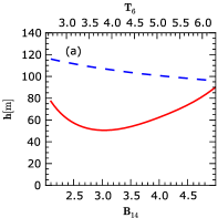
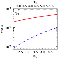
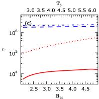
Figure 3.13: Dependence of the gap height (panel a), the screening factor or the overheating parameter (panel b), and the particle Lorentz factor (panel c) on the surface magnetic field. Solid red lines correspond to the PSG-on mode (ICS-dominated gaps) while dashed blue lines correspond to the PSG-off mode (CR-dominated gaps). Calculations were performed using the following parameters: $P=0.23$, $\Re_{6}=0.6$, $B_{{\rm d}}=1.2\times 10^{12}\,{\rm G}$, and $\alpha=36^{\circ}$. The actual polar cap radius was calculated separately for a given surface magnetic field as $R_{{\rm pc}}=R_{{\rm dp}}\sqrt{B_{{\rm d}}/B_{{\rm s}}}$. In panel (c) the red solid and dotted lines correspond to characteristic and maximum Lorentz factors ($\gamma_{{\rm c}}$, $\gamma_{{\rm max}}$) in the PSG-on mode while blue dashed and dashed-dotted lines correspond to $\gamma_{{\rm c}}$ and $\gamma_{{\rm max}}$ in the PSG-off mode. Corresponding critical temperature is shown on top axis of the figures.

3.3.2 Influence of the curvature radius

The curvature of the magnetic field lines significantly affects the gap height in the PSG-off mode (see Figure 3.14, panel a). In the case of the CR-dominated gap, the curvature of the magnetic field lines affects not only the photons’ mean free path (for higher curvature the magnetic field will absorb photons faster), but also the particle mean free path and, more importantly, the energy of photons generated in the gap region. The higher energy of photons further reduces the photon mean free path, thus resulting in lower heights of the PSG. In contrast, the gap height in the PSG-on mode is only slightly affected by changes in the curvature of the magnetic field lines. In this case the most important parameter which determines the cascade properties is the primary particle mean free path which does not depend on the curvature of the magnetic field lines.

The overheating parameter in the PSG-off mode inversely depends on the radius of curvature of the magnetic field lines (see Figure 3.14, panel b). The higher the curvature, the higher the overheating parameter, which means that the sparks are narrower. This is consistent with the expectation that for a higher curvature of the magnetic field lines, the gap breakdown is easier to develop and takes place before the sparks manage to grow in width. On the other hand, the screening factor in the PSG-off mode does not depend on the curvature of the magnetic field lines.

With an increasing radius of curvature the Lorentz factor of primary particles (both $\gamma_{{\rm c}}$ and $\gamma_{{\rm max}}$) required to close the gap in the PSG-off mode also increases. This reflects the fact that in order to produce a sufficient number of photons in the gap region, the primary particles should be accelerated to higher energies (if the curvature is lower). Higher energies of the primary particles will increase the emitted $\gamma$-photon energy, thereby they will partly inhibit the growth of the photon mean free path due to the lower curvature. As mentioned above, the gap height in the PSG-on mode very weakly depends on the photon mean free path, thus both $\gamma_{{\rm c}}$ and $\gamma_{{\rm max}}$ are not affected by the increase in the radius of curvature.

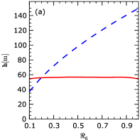
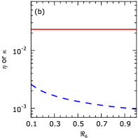
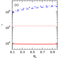
Figure 3.14: Dependence of the gap height (panel a), the screening factor or the overheating parameter (panel b), and the particle Lorentz factor (panel c) on the curvature radius of magnetic field lines. Calculations were performed using the following parameters: $P=0.23$, $B_{{\rm d}}=1.2\times 10^{12}\,{\rm G}$, $B_{{\rm s}}=2.4\times 10^{14}\,{\rm G}$, $\alpha=36^{\circ}$. For a more detailed description see Figure 3.13.

3.3.3 Influence of the pulsar period

As we can see from Figure 3.15, panel (a) and panel (c), in the PSG-on mode the gap height and the Lorentz factor of primary particles do not depend on the pulsar period. The increase in the screening factor (see Figure 3.15b) compensates the increase in the acceleration potential drop (see Equation 3.8). Thus the particles in the gap region are accelerated in the same way independently of the pulsar period. On the other hand, the gap height in the PSG-off mode increases with the increasing pulsar period. This reflects the fact that in the PSG-off mode the acceleration potential, and hence $\gamma_{{\rm c}}$ and $\gamma_{{\rm max}}$, decreases with longer periods (see Equation 3.26). Longer pulsar periods entail an increase in the screening factor (in the PSG-on mode, see Equation 3.39) and in the overheating parameter (in the PSG-off mode). Note that for periods longer than some specific value (for a given pulsar’s parameters it is $P_{{\rm max}}\approx 9\,{\rm s}$), the screening factor in the PSG-on mode would exceed unity. This means that the PSG-on mode cannot be responsible for the gap breakdown for pulsars with such long periods.

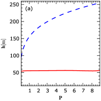
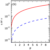
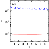
Figure 3.15: Dependence of the gap height (panel a), the screening factor or a overheating parameter (panel b), and the particle Lorentz factor (panel c) on the pulsar period. Calculations were performed using the following parameters: $P=0.23$, $B_{{\rm d}}=1.2\times 10^{12}\,{\rm G}$, $B_{{\rm s}}=2.4\times 10^{14}\,{\rm G}$, $\alpha=36^{\circ}$, $\Re_{6}=0.6$. The actual polar cap radius was calculated separately for a given pulsar period as $R_{{\rm pc}}=R_{{\rm dp}}\sqrt{B_{{\rm d}}/B_{{\rm s}}}$, where $R_{{\rm dp}}=\sqrt{2\pi R^{3}/\left(cP\right)}$. For a more detailed description see Figure 3.13.

3.4 Drift model

The existence of IAR in general causes a rotation of the plasma relative to the NS, as the charge density differs from the Goldreich-Julian co-rotational density. The power spectrum of radio emission must have a feature due to this plasma rotation. This feature is indeed observed and is called the drifting subpulse phenomenon.

3.4.1 Aligned pulsars

An explanation for drifting subpulses was offered by Ruderman and Sutherland, (1975) as being due to a rotating carousel of sub-beams within a hollow emission cone. According to this model a pair cascades may not occur simultaneously across the whole polar cap but is localised in the form of discharges of small regions in the polar gap. Such sparks may produce plasma columns that stream into the magnetosphere to produce the observed radio emission. The location of the discharges on the polar cap determines the geometrical pattern of instantaneous subpulses within a pulsar’s integrated pulse profile.

In the PSG model the stable pattern of subpulses is due to heating of the inactive part of the spark (the place where no cascade forms due to a low acceleration potential) by all the neighbouring discharges. The lifetime of a single spark is very short. On the other hand, an inactive region is continuously heated by all the neighbouring sparks. Even when one of them dies, the temperature is still high enough (high ion density) to prevent spark formation in this region. As the discharges do not exchange information (they are not synchronised) and their lifetime is very small, the geometrical pattern of sparks on the polar cap should be stable.

For pulsars with an aligned magnetic and rotation axis the sparks circulate around the rotation axis. Note that this circulation is not related with the magnetic axis but with the direction of the co-rotational velocity. Namely, the drift velocity is opposed to the co-rotational velocity.

We can calculate the drift velocity of an aligned pulsar using the following approximation (see Figure 3.16)

$$v_{{\rm dr}}\approx\frac{2\pi R_{{\rm pc}}}{PP_{3}}\frac{\beta}{\rho}\frac{P_{2}^{\circ}}{360^{\circ}},$$ (3.42)

where $R_{{\rm pc}}$ is the actual polar cap size, $P_{2}^{\circ}$ is the characteristic spacing between subpulses in the pulse longitude, $P_{3}$ is the period at which a pattern of subpulses crosses the pulse window (in units of the pulsar period), $\beta$ is the impact angle, and $\rho$ is the opening angle.

Figure 3.16: Top view of a polar cap region of an aligned pulsar. Small circles represent sparks, while the red line corresponds to the line of sight. If we neglect the transition from a non-dipolar structure of the magnetic field on the stellar surface to a dipolar structure in the region where radio emission is produced, we can assume that the observed subpulse separation $P_{2}^{\circ}$ also describes spark separation $\varrho_{s}$ (angular separation between the adjacent sparks on the polar cap).

In such an approximation the assumption that only half of the spark is active can be written as

$$\frac{P_{2}^{\circ}}{360^{\circ}}\approx\frac{2h_{\perp}}{2\pi R_{{\rm pc}}\frac{\beta}{\rho}}.$$ (3.43)

Finally, we can define the observed drift velocity of aligned pulsars as

$$v_{dr}\approx\frac{2h_{\perp}}{PP_{3}}.$$ (3.44)

3.4.2 Non-aligned pulsars

Most observed pulsars are non-aligned rotators. It is very common to apply the carousel model to interpret observations of the drifting subpulses of non-aligned pulsars (Ruderman and Sutherland,, 1975). Despite the fact that the carousel model can explain some properties of subpulses (for example the change in intensity), we believe that this model is not suitable for describing the spark’s behaviour on the polar cap. There is no physical reason for a spark to circulate around the magnetic axis. The circulation in aligned pulsars is caused by a lack of coronation with respect to the rotation axis. For non-aligned pulsars, the co-rotation velocity in the polar cap region has more or less the same direction: what is more, if we assume circulation around the magnetic axis we will get plasma with a velocity that is higher than the co-rotational velocity, which is difficult to explain in a region where the charge density is lower than the co-rotational density.

As in our model, the drift is caused by a lack of charge in IAR, thus the plasma should drift in approximately the same direction, i.e. in the direction opposite to the co-rotation velocity. We believe that the change in subpulse intensity is caused by the observation of a different part of a spark and/or different conditions across the polar cap at which the spark is formed (e.g. magnetic field strength, curvature of the magnetic field lines, background photon flux).

For pulsars with a relatively high inclination angle $\alpha$ we can calculate the drift velocity using the following approximation

$$v_{dr}\approx\frac{2R_{{\rm pc}}\frac{W}{W_{\beta 0}}}{PP_{3}}\frac{P_{2}^{\circ}}{W}\approx\frac{2R_{{\rm pc}}}{PP_{3}}\frac{P_{2}^{\circ}}{W_{\beta 0}},$$ (3.45)

where $W$ is the profile width and $W_{\beta 0}\approx W/\sqrt{1-\left(\frac{\beta}{\rho}\right)^{2}}$ is the profile width calculated assuming $\beta=0$ (see Figure 3.17). Using the assumption that only half of the spark is active, we can write that

$$\frac{P_{2}^{\circ}}{W}\approx\frac{2h_{\perp}}{2R_{{\rm pc}}\frac{W}{W_{\beta 0}}}\longrightarrow\frac{P_{2}^{\circ}}{W_{\beta 0}}\approx\frac{h_{\perp}}{R_{{\rm pc}}},$$ (3.46)

and the drift velocity

$$v_{dr}=\frac{2h_{\perp}}{PP_{3}}.$$ (3.47)

The spark half-width can be calculated using Equation 3.46 as follows

$$h_{\perp}=R_{{\rm pc}}\frac{P_{2}^{\circ}}{W_{\beta 0}}.$$ (3.48)

Figure 3.17: Top view of the polar cap region in the case of a non-aligned pulsar. Small circles represent sparks, the red line corresponds to the line of sight. In general, the observed subpulse separation $P_{2}^{\circ}$ does not describe the actual spark separation $\varrho_{s}$ (the angular separation between the adjacent sparks on the polar cap). In order to calculate the distance between the sparks we use an approximation from Equation 3.45.

3.4.3 Screening factor

In our model the drift is caused by a lack of charge in IAR, thus we can write the equation for the drift velocity as follows

$${\bf v_{\perp}={\bf v}}_{{\rm dr}}=\frac{c{\bf\Delta E}\times{\bf B}}{B^{2}},$$ (3.49)

where $\Delta{\bf E}$ is the electric field caused by the difference of an actual charge density from the Goldreich-Julian co-rotational density. We can a use calculation of the circulation of an electric field, Equations 3.20 and 3.26, to find the dependence of the drift velocity on the screening factor:

$$v_{{\rm dr}}=c\frac{E_{\theta}B_{r}}{B_{r}^{2}}=\frac{4\pi\eta h_{\perp}\cos\alpha}{P}.$$ (3.50)

Finally, by using Equations 3.47 and 3.50 we can find the dependence of the screening factor on the observed drift parameters

$$\eta=\frac{1}{2\pi P_{3}\cos\alpha}.$$ (3.51)

3.4.4 Profile width and subpulse separation

The key parameters in the above calculations are the pulse width $W$ (or $W_{\beta 0}$), the characteristic spacing between subpulses $P_{2}^{\circ}$, and the period at which a pattern of subpulses crosses the pulse window $P_{3}$. Of these three only $P_{3}$ is easy to apply, both $W$ and $P_{2}^{\circ}$ need serious study before they can be used.

In general, the profile width depends on the frequency at which we observe the pulsar, and most normal pulsars show a systematic increase in pulse width and the separation of profile components when observed at lower frequencies. The model known as radius-to-frequency mapping explains this effect as a direct consequence of the emission at higher frequencies being produced closer to the neutron star surface than at lower frequencies. For this reason both the pulse width and the spacing between subpulses should be measured at the same frequency. Note that $P_{3}$ is not affected by this effect since its determination involves analyses of many pulses and does not depend on the pulse width. The observed pulse width $W$, measured in longitude of rotation, can be calculated by applying simple spherical geometry (Gil et al.,, 1984):

$$\sin^{2}\frac{W}{4}=\frac{\sin^{2}\left(\rho/2\right)-\sin^{2}\left(\beta/2\right)}{\sin\alpha\sin\left(\alpha+\beta\right)}.$$ (3.52)

In the above calculations we are using the $W_{\beta 0}\approx W/\sqrt{1-\left(\frac{\beta}{\rho}\right)^{2}}$approximation, where $W_{\beta 0}$ is the pulse width calculated assuming $\beta=0$. In the first approximation we can assume that $W_{\beta 0}$ corresponds to the distance $2R_{{\rm pc}}$ at the polar cap which, is valid for non-aligned pulsars with a relatively high inclination angle. A more accurate value can be calculated using formulas presented in Gil et al., (1984). The running polar coordinates along the line of sight trajectory can be expressed in the form

$$\rho\left(\varphi\right)=2\arcsin\left(\sqrt{\sin^{2}\frac{\varphi}{2}\sin\alpha\sin\left(\alpha+\beta\right)+\sin^{2}\frac{\beta}{2}}\right),$$ (3.53)

$$\sigma\left(\varphi\right)=\arctan\left(\frac{\sin\varphi\sin\alpha\sin\left(\alpha+\beta\right)}{\cos\left(\alpha+\beta\right)-\cos\alpha\cos\rho\left(\varphi\right)}\right).$$ (3.54)

In numerical calculations of $\sigma\left(\varphi\right)$ it is convenient to use the “${\rm atan2}$” function which takes into account the signs of both components and places the angle in the correct quadrant (see the footnote on page 1). Figure 3.18 presents the geometry of the emission region for pulsars with available radio observations of the subpulse drift and X-ray observations of the hot spot. By knowing the actual polar cap radius $R_{{\rm pc}}$ we can determine the transverse size of the region responsible for the generation of plasma clouds in IAR (the spark half-width).

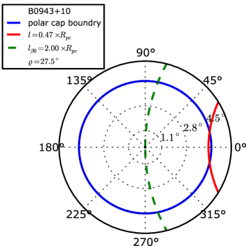
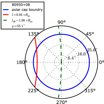
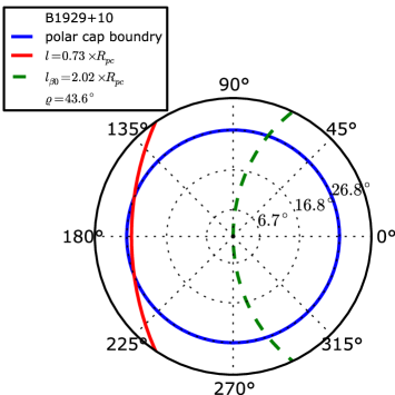
Figure 3.18: Top view of the polar cap region of pulsars with radio drift observations and X-ray hot spot radiation. Red lines correspond to the line of sight while green dashed lines correspond to the theoretical lines of sight calculated with an assumption that $\beta=0^{\circ}$. The geometry of pulsars can be found in Table 1.3.

In our model the motion of sparks and the progressively different positions of the associated plasma columns are responsible for the observed drift of subpulses. For some pulsars it is possible to measure directly the subpulse separation using a single pulse. In most calculations it is assumed that the observed subpulses correspond to the adjacent sparks. In general, this is not necessarily true. The distribution of sparks on the polar cap is unknown and it is very likely that the line of sight does not cross the adjacent sparks but it omits some sparks in between. Therefore, the observed value of $P_{2}^{\circ}$ should be considered rather as an upper limit for spark separation. Furthermore, for many pulsars the observed value $P_{2}^{\circ}>W$, which means that it is not related to any structure at the polar cap but that it corresponds to some other periodicity. We can use Equations 3.39 and 3.51 to calculate the spark half-width as follows

$$h_{\perp}=26.2\frac{\left(B_{14}^{1.1}+0.3\right)^{2}PP_{3}\sqrt{\left|\cos\alpha\right|}}{B_{14}}.$$ (3.55)

Finally, using Equation 3.46 we can determine the predicted value of the subpulse separation

$$\tilde{P}_{2}^{\circ}\approx\frac{26.2\left(B_{14}^{1.1}+0.3\right)^{2}PP_{3}\sqrt{\left|\cos\alpha\right|}}{B_{14}R_{{\rm pc}}}W_{\beta 0}.$$ (3.56)

3.4.5 Heating efficiency

The spin-down energy loss is

$$L_{{\rm SD}}=3.9\times 10^{31}\frac{\dot{P}_{-15}}{P^{3}}.$$ (3.57)

We can use Equations 3.26, 3.48 and 3.51 to calculate the dependence of the acceleration potential drop on the parameters of drifting subpulses:

$$\Delta V\approx 2.824\times 10^{10}\left(\frac{\dot{P}_{-15}}{P^{3}}\right)^{0.5}\frac{1}{P_{3}}\left(\frac{P_{2}^{\circ}}{W_{\beta 0}}\right)^{2}.$$ (3.58)

The power of heating by backstreaming particles can be calculated as follows

$$L_{{\rm heat}}=\eta n_{{\rm GJ}}c\left(\Delta Ve\right)\pi R_{{\rm pc}}^{2}.$$ (3.59)

The number density of the Goldreich-Julian co-rotational charge can be calculated using

$$n_{{\rm GJ}}=\frac{{\bf\Omega}\cdot{\bf B_{{\rm s}}}}{2\pi ce},$$ (3.60)

where $\Omega=2\pi/P$ is an angular velocity, $B_{{\rm s}}=bB_{{\rm d}}$ is the surface magnetic field, $b=R_{dp}^{2}/R_{pc}^{2}$, $B_{{\rm d}}=2.02\times 10^{12}\sqrt{P\dot{P}_{-15}}\,{\rm G}$, and $R_{{\rm dp}}=\sqrt{2\pi R^{3}/\left(cP\right)}\approx 1.45\times 10^{4}P^{-0.5}$. The Goldreich-Julian density in terms of observed parameters can be written as

$$n_{{\rm GJ}}=2.9\times 10^{19}\left(P^{-3}\dot{P}_{-15}\right)^{1/2}\frac{\cos\alpha}{R_{{\rm pc}}^{2}}.$$ (3.61)

Finally, using Equations 3.51, 3.58 and 3.61 we can estimate the dependence of the heating power and thus the X-ray luminosity of the hot spot radiation on the parameters of radio observations as follows

$$L_{{\rm heat}}=L_{{\rm X}}=6\times 10^{30}\left(\frac{\dot{P}_{-15}}{P^{3}}\right)\left(\frac{1}{P_{3}}\frac{P_{2}^{\circ}}{W_{\beta 0}}\right)^{2}.$$ (3.62)

The heating efficiency by the backstreaming particles can be calculated as

$$\xi_{{}_{{\rm heat}}}=\frac{L_{{\rm heat}}}{L_{{\rm SD}}}=0.15\left(\frac{1}{P_{3}}\frac{P_{2}^{\circ}}{W_{\beta 0}}\right)^{2}.$$ (3.63)

3.4.6 Ion luminosity

In the PSG-on mode the bulk of energy is transferred to the iron ions which shield the acceleration potential drop. Similar as for the backstreaming particles, we can estimate the power of ion acceleration as

$$L_{{\rm ion}}=\left(1-\eta\right)n_{{\rm GJ}}c\left(\Delta Vq_{{\rm ion}}\right)\pi R_{{\rm pc}}^{2},$$ (3.64)

where $q_{{\rm ion}}=26e=1.25\times 10^{-8}\,{\rm erg^{0.5}cm^{0.5}}$ is the ion charge. Using the same approach as for electron, we can calculate the dependence of energy transformed to the ions per second on the parameters of the radio observations as follows

$$L_{{\rm ion}}=9.75\times 10^{32}\left(1-\eta\right)\frac{\dot{P}_{-15}}{P^{3}P_{3}}\left(\frac{P_{2}^{\circ}}{W_{\beta 0}}\right)^{2}\cos\alpha.$$ (3.65)

It is clearly visible that if the screening factor is low $\eta\ll 1$, most of the energy in IAR is transferred to the iron ions. Using Equations 3.59 and 3.64 we can show that

$$\frac{L_{{\rm ion}}}{L_{{\rm heat}}}=\frac{26\left(1-\eta\right)}{\eta}\approx\frac{26}{\eta}.$$ (3.66)

Finally, the ion acceleration efficiency can be calculated as

$$\xi_{{\rm{}_{ion}}}=\frac{L_{{\rm ion}}}{L_{{\rm SD}}}\approx 25\frac{1}{P_{3}}\left(\frac{P_{2}^{\circ}}{W_{\beta 0}}\right)^{2}\cos\alpha.$$ (3.67)

It may seem that ion luminosity exceeds the spin-down luminosity, but note that both $P_{3}>1$ and $P_{2}^{\circ}<W_{\beta 0}$. The predicted values of heating efficiency $\xi_{{\rm heat}}$ and ion acceleration efficiency $\xi_{{\rm ion}}$ are presented in the next section.

3.4.7 Observations

In this section we confront the values of the subpulse drift and X-ray radiation as estimated by other authors with predicted values estimated using the approach presented above. In Table 3.2, alongside our predicted value of $\tilde{P}_{2}^{\circ}$ we present two other estimates: (1) the subpulse separation estimated using the carousel model developed by Ruderman and Sutherland, (1975), $P_{2,{\rm RS}}^{\circ}$; (2) the subpulse separation found using the analysis of the Longitude-Resolved Fluctuation Spectrum (Backer,, 1970) and the integrated Two-Dimensional Fluctuation Spectrum (Edwards and Stappers,, 2003), performed by Weltevrede et al., (2006), $P_{2,{\rm W}}^{\circ}$. We have found that the subpulse separation estimated using the fluctuations spectra is overestimated (in most cases $P_{2,{\rm W}}^{\circ}>W$). By definition $P_{2}^{\circ}$ should correspond to the structure within a single pulse, thus if the geometry is not extreme ($\varrho>1^{\circ}$) it should comply with $P_{2}^{\circ}\leq W$. For this specific sample of pulsars $P_{2,{\rm W}}^{\circ}$ should not be interpreted as the actual subpulse separation. On the other hand, $\tilde{P}_{2}^{\circ}$ is in good agreement with $P_{2,{\rm RS}}^{\circ}$. The predicted values $\tilde{P}_{2}^{\circ}$ for B0834+06 and B0943+10 suggest that $P_{2,{\rm RS}}^{\circ}$ for those pulsars could be overestimated due to the aliasing phenomenon ($P_{2,{\rm RS}}^{\circ}\approx 2\tilde{P}_{2}^{\circ}$). For B1929+10 we do not list $P_{2,{\rm RS}}^{\circ}$ as its value presented in Gil et al., (2008) does not comply with the $P_{2,{\rm RS}}^{\circ}\leq W$ condition. We believe that the overestimated value of $P_{2,{\rm RS}}^{\circ}$ for B1929+10 is a result of using the fluctuations spectra presented in Weltevrede et al., (2006) to calculate the number of sparks in the carousel model. Note that the coincidence of $\tilde{P}_{2}^{\circ}$ and $P_{2,{\rm RS}}^{\circ}$ is yet to be clarified, as in our model there is no physical reason for sparks to circulate around the magnetic axis. In fact, the PSG model assumes the non-dipolar structure of the magnetic field lines in the gap region and the actual position of the polar cap is not necessarily coincident with the global dipole (e.g. see Figures 2.6, 2.18, 2.24).

Table 3.2: Details of a subpulse drift for pulsars with X-ray hot spot radiation. The individual columns are as follows: (1) Pulsar name, (2) Predicted characteristic spacing between subpulses in the pulse longitude, $\tilde{P}_{2}^{\circ}$; (3) Spacing between subpulses, found in the literature, estimated using the carousel model, $P_{2,{\rm RS}}^{\circ}$; (4) Spacing between subpulses estimated using fluctuations spectra, $P_{2,{\rm W}}^{\circ}$; (5) Period at which a pattern of subpulses crosses the pulse window (in units of the pulsar period), $P_{3}$; (6) Number of sparks estimated using the carousel model, $N$; (7) Profile width at 10%, $W$; (8) Profile width calculated assuming $\beta=0$, $W_{\beta 0}$; (9) Angular width of the observed region on the polar cap $\varrho$ (see Figure 3.18); (10) References; (11) Number of the pulsar.

Name	$\tilde{P}_{2}^{\circ}$	$P_{2,{\rm RS}}^{\circ}$	$P_{2,{\rm W}}^{\circ}$	$P_{3}$	$N$	$W$	$W_{\beta 0}$	$\varrho$	Ref.	No.
	$\left({\rm deg}\right)$	$\left({\rm deg}\right)$	$\left({\rm deg}\right)$	$\left(P\right)$		$\left({\rm deg}\right)$	$\left({\rm deg}\right)$	$\left({\rm deg}\right)$
B0628–28	$8.4$	$6$	$30$	$7.0$	$24$	$38.1$	$48.2$	$98.0$	Gi07, We06	$8$
B0834+06	$1.4$	$3$	$20$	$2.2$	$14$	$12.2$	$15.8$	$105.5$	Ra07, We06	$14$
B0943+10	$9.8$	$17$	–	$1.8$	$20$	$25.6$	$84.7$	$27.5$	De99, De01, As01	$15$
B0950+08	$4.0$	–	–	$6.5$	–	$32.2$	$63.7$	$55.1$	Wo80	$16$
B1133+16	$3.2$	$4$	$130$	$3.0$	$11$	$14.4$	$18.1$	$107.9$	Gi06, He07, We06	$22$
B1929+10	$5.8$	$?$	$90$	$9.8$	$?$	$24.5$	$80.8$	$43.6$	Gi08, We06	$42$

Table 3.3 presents the observed and derived parameters of PSG for pulsars with available radio and X-ray observations. In the calculations we used the predicted value of subpulse separation $\tilde{P_{2}^{\circ}}$. Note that we consider only pulsars with a visible hot spot component since only for these pulsars we can estimate the size of the polar cap. The low value of the estimated screening factor ($\eta\ll 1$) suggests that when the drift is visible, the pulsar operates in the PSG-on mode. If the pulsar operates in the PSG-off mode, $\eta\approx 1$, the drift velocity is much higher (see Equation 3.50) and the drift phenomenon should be more chaotic and much difficult to identify. Observations of PSR 0943+10 show a strong, regular subpulse drifting in the radio-bright mode, with only a hint of modulation in the radio-quiescent mode. Based on this fact we believe that the two different scenarios of the gap breakdown (PSG-on and PSG-off modes) can explain the mode changing.

Table 3.3: Derived parameters of PSG for pulsars with available radio observations of the subpulse drift and X-ray hot spot radiation. The individual columns are as follows: (1) Pulsar name, (2) Screening factor, $\eta$; (3) Predicted heating efficiency, $\xi_{{\rm heat}}$; (4) Observed bolometric efficiency, $\xi_{{}_{{\rm BB}}}$; (5) Predicted ion acceleration efficiency, $\xi_{{\rm{}_{ion}}}$; (6) Surface temperature, $T_{{\rm s}}$; (7) Strength of the surface magnetic field, $B_{{\rm s}}$; (8) Observed polar cap radius, $R_{{\rm pc}}$; (9) Estimated spark half-width, $h_{\perp}$; (10) Number of the pulsar. $T_{{\rm s}}$, $R_{{\rm pc}}$, $b$ were chosen to fit $1\sigma$ uncertainty. Note that in the calculations $\tilde{P}_{2}^{\circ}$ was used.

Name	$\eta$	$\log\xi_{{}_{{\rm heat}}}$	$\log\xi_{{}_{{\rm BB}}}$	$\log\xi_{{}_{{\rm ion}}}$	$T_{{\rm s}}$	$B_{{\rm s}}$	$R_{{\rm pc}}$	$h_{\perp}$	No.
		$\left({\rm radio}\right)$	$\left({\rm x-ray}\right)$	$\left({\rm ions}\right)$	$\left(10^{6}{\rm K}\right)$	$\left(10^{14}{\rm G}\right)$	$\left({\rm m}\right)$	$\left({\rm m}\right)$
B0628–28	$0.07$	$-4.03$	$-3.61$	$-1.43$	$2.5$	$2.0$	$23$	$3.9$	$8$
B0834+06	$0.15$	$-3.60$	$-3.34$	$-1.35$	$3.0$	$2.4$	$20$	$1.8$	$14$
B0943+10	$0.09$	$-3.24$	$-3.27$	$-0.75$	$3.3$	$2.5$	$17$	$2.0$	$15$
B0950+08	$0.09$	$-5.08$	$-4.54$	$-2.62$	$2.6$	$2.1$	$14$	$0.7$	$16$
B1133+16	$0.09$	$-3.29$	$-3.13$	$-0.81$	$3.4$	$2.7$	$17$	$2.9$	$22$
B1929+10	$0.02$	$-5.10$	$-4.17$	$-1.98$	$4.2$	$2.0$	$22$	$1.6$	$42$

Chapter 4 Cascade simulation

In this chapter we present the approach of calculating the pair cascades developed by Medin and Lai, (2010) which has been applied to cases with non-dipolar structure of magnetic field. The original approach was adapted to perform full three-dimensional calculations and extended with effects that may have a greater importance for non-dipolar configuration of surface magnetic fields (e.g. aberration). Additionally, to perform a thorough analysis of the Inverse Compton Scattering we present the detailed description of calculating the ICS cross section originally developed by Gonthier et al., (2000).

Following the approach presented by Medin and Lai, (2010) we can divide the cascade simulation into three parts:

• propagation of the primary particle (including photon emission),

• photon propagation in strong magnetic field (pair production, photon splitting),

• propagation and photon emission of the secondaryparticles.

We use the ”co-rotating” frame of reference (the frame which rotates with the star) to track both photons and particles. In calculations we consider regions far inside the light cylinder. Thus, following Medin and Lai, (2010), we ignore any bending of the photon path due to rotation of the star. Furthermore, we also ignore effects of general relativity on trajectories of photons and particles.

Figure 4.1 presents a summary flowchart of the algorithm used to calculate the properties of secondary plasma and the spectrum of radiation for a given structure of a neutron’s star magnetic field and gap parameters.

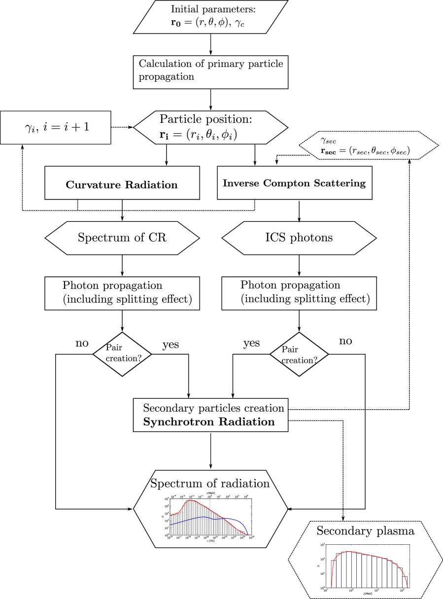
Figure 4.1: Flowchart of algorithm used to calculate a cascade simulation.

4.1 Curvature Radiation

As we have shown in Chapter 2, an ultrastrong surface magnetic field ($B_{{\rm s}}>10^{14}\,{\rm G}$) is accompanied by high curvature (curvature radius $\Re_{6}\approx 0.1-10$). This suggests that one of the important processes of radiation which should be considered is Curvature Radiation (CR).

CR is quite similar to ordinary synchrotron radiation (radiation of ultrarelativistic particles in the magnetic field), the only difference being that the radius of circular motion (the gyroradius) is in fact the curvature radius of magnetic field lines. Due to beaming effects the radiation appears to be concentrated in a narrow set of directions about the velocity of the particle. The angular width of the cone of emission is of the order $\sim 1/\gamma$, where $\gamma$ is a Lorentz factor of an emitting particle (for more details see Rybicki and Lightman,, 1979).

We track the primary particle above the acceleration zone (the gap region) as it moves along the magnetic field line. The length of the step $\Delta s$ is chosen so as to achieve sufficient accuracy even for large curvature of the magnetic field line, $\Delta s\approx 0.01\Re_{{\rm min}}$, where $\Re_{{\rm min}}$ is the minimum radius of curvature. The distribution of CR photon energy can be written as (see Equation 14.93 in Jackson,, 1998)

$$\frac{{\rm d}N}{{\rm d}\epsilon}=\frac{E}{\epsilon_{{\rm{}_{CR}}}}\frac{9\sqrt{3}}{8\pi}\int_{\epsilon/\epsilon_{{}_{{\rm CR}}}}^{\infty}K_{5/3}(t){\rm d}t,$$ (4.1)

where $E=4\pi e^{2}\gamma^{4}/3\Re$ is the total energy radiated per revolution, $\epsilon_{{}_{{\rm CR}}}=3\gamma^{3}\hbar c/(2\Re)$ is the characteristic energy of curvature photons, and $K_{5/3}$ is the $n=5/3$ Bessel function of the second kind. The total energy radiated by a particle after it passes the length $\Delta s$, $E_{{}_{\Delta s}}$, can be written as

$$E_{{}_{\Delta s}}=E\frac{\Delta s}{2\pi\Re}.$$ (4.2)

Thus, by using Equations 4.1 and 4.2 we can write the formula for the distribution on CR photon energy after a particle passes length $\Delta s$

$$\frac{{\rm d}N}{{\rm d}\epsilon}=\frac{\Delta s}{2\pi\Re}\frac{\sqrt{3}e^{2}\gamma}{\hbar c}\int_{\epsilon/\epsilon_{{\rm{}_{CR}}}}^{\infty}K_{5/3}(t){\rm d}t.$$ (4.3)

It is convenient to divide the spectrum of photon energy into discrete bins. Then, the number of photons in each energy bin can be calculated as

$$N_{\epsilon}=\int_{\epsilon_{{}_{i}}}^{\epsilon_{{}_{i}}+\Delta\epsilon}\frac{dN}{d\epsilon}{\rm d}\epsilon,$$ (4.4)

where $\epsilon_{{}_{i}}$ is the lowest energy for the $i$-th bin and $\Delta\epsilon$ is the energy bin width. Our simulation uses $50$ bins with an energy range of $\epsilon_{{}_{0}}=4\times 10^{-2}\,{\rm keV}$ (soft X-ray) to $\epsilon_{{}_{49}}=4\times 10^{5}\,{\rm MeV}$ (hard $\gamma$-rays).

Depending on the photon frequency the polarisation fraction of CR photons is between $50\%$ and $100\%$ polarised parallel to the magnetic field (see Jackson,, 1998, Rybicki and Lightman,, 1979). Therefore, using similar approach as Medin and Lai, (2010) we randomly assign the polarisation in the ratio of one photon $\perp$-polarised to every seven $\parallel$-polarised photons, which corresponds to $75\%$ parallel polarisation.

4.2 Photon propagation

To explain some of the properties of pulsars and their surroundings (e.g. nebulae radiation), large magnetospheric plasma densities exceeding the Goldreich-Julian density (see Equation 3.7) by many orders of magnitude are required. In order to simulate the process of generation of such a dense plasma it is necessary to check the conditions of photon decay into electron-positron pairs.

A photon with energy $E_{\gamma}>2mc^{2}$ and propagating with a nonzero angle $\Psi$ with respect to an external magnetic field can be absorbed by the field and, as a result an electron-positron pair is created. The concurrent process is photon splitting $\gamma\rightarrow\gamma\gamma$, which may occur even if the photon energy is below the pair creation threshold ($E_{\gamma}<2mc^{2}$).

In the cascade simulation the photon is emitted (or scattered in the case of ICS) from point $P_{{\rm ph}}$ in a direction tangent to the magnetic field line $\Delta\mathbf{s_{\parallel}}$. The direction vector is calculated as the value of the magnetic field at the point of photon creation (see Equations 2.1, 2.2 and 2.7) normalised so that its length is equal to the desired step $\Delta\mathbf{s_{\parallel}}=\mathbf{B}\Delta s/B$. However, the direction of the magnetic field at the point of photon emission does not take into account the randomness of the emission direction due to the relativistic beaming effect. In Section 4.2.1 we describe a procedure to include the beaming effect in the emission process which alters $\Delta\mathbf{s_{\parallel}}\rightarrow{\bf\Delta s_{ph}}$. Finally, we can write that at the point of curvature emission photons are created with energy $\epsilon_{{\rm ph}}$, polarisation $\parallel$ or $\perp$, weighting factor $N_{\epsilon}$ (number of photons), and with both optical depths (for pair production $\tau$ and for photon splitting $\tau_{{\rm sp}}$) set to zero. Since we neglect any banding of the photon path we assume that from the point of emission it travels in a straight line. In each following step the photon travels a distance ${\bf\Delta s_{ph}}$. In the co-rotating frame of reference in every step we need to take into the account aberration due to pulsar rotation. In order to do so, in every step we alter the photon position according to the procedure described in Section 4.2.2. As stated by Medin and Lai, (2010) we can calculate the change in the pair production optical depth , $\Delta\tau$, and in the photon splitting optical depth $\Delta\tau_{{\rm sp}}$, at the new position as:

$$\Delta\tau\simeq\Delta s_{{\rm ph}}R_{\|,\perp},$$ (4.5)

$$\Delta\tau_{{\rm sp}}\simeq\Delta s_{{\rm ph}}R_{\|,\perp}^{{\rm sp}},$$ (4.6)

where $R_{\|,\perp}$ and $R_{\|,\perp}^{{\rm sp}}$ are the attenuation coefficients for $\|$ or $\perp$ polarised photons for pair production and photon splitting, receptively.

4.2.1 Relativistic beaming (emission direction)

Due to relativistic beaming the emission direction should be modified by an additional emission angle of order $\sim 1/\gamma$. We use the following steps to include the beaming effect in our simulation (see Figure 4.2).

(I) The first step is rotation of the $xyz$ frame of reference in order to align the $z$-axis with $\mathbf{\Delta s_{\parallel}}$. In our calculations we used rotation by angle $\varsigma_{y}$ around the $y$-axis, $R_{y}\left(\varsigma_{y}\right)$, and rotation by angle $\varsigma_{x}$ around the $x$-axis, $R_{x}\left(\varsigma_{x}\right)$. The final rotation matrix can be written as

$$R_{yx}=R_{y}\left(\varsigma_{y}\right)R_{x}\left(\varsigma_{x}\right)=\left[\begin{array}[]{ccc}\cos\varsigma_{y}&\sin\varsigma_{x}\sin\varsigma_{y}&\sin\varsigma_{y}\cos\varsigma_{x}\\ 0&\cos\alpha&-\sin\alpha\\ -\sin\varsigma_{y}&\cos\varsigma_{y}\sin\varsigma_{x}&\cos\varsigma_{y}\cos\varsigma_{x}\end{array}\right].$$ (4.7)

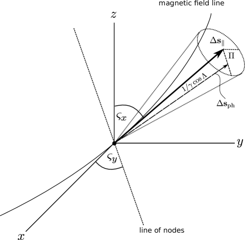
Figure 4.2: Relativistic beaming effect of photon emission (for both CR and ICS). In the simulation we include the beaming effect by performing three steps: (I) rotation of the $xyz$ frame of reference in order to align the $z$-axis with $\mathbf{\Delta s_{\parallel}}$, (II) transformation of the step vector from a Cartesian to a spherical system of coordinates and alteration of the $\theta$ and $\phi$ components with random values $1/\gamma\cos\Lambda$ and $\Pi$, respectively, (III) transformation of the step vector from a spherical to a Cartesian system of coordinates and rotation back to the original system of reference. Note that after these steps we get a new vector ${\bf\Delta s_{ph}}$ inclined to the primary one, ${\bf\Delta s_{ph}}$, at an angle ranging from $0$ to $1/\gamma$.

The Euler angles for rotations can be calculated as

$$\begin{array}[]{c}\varsigma_{x}={\rm atan2}\left(s_{y},s_{z}\right),\\ \varsigma_{y}=\begin{cases}\arctan\left(-\frac{s_{x}}{s_{z}}\cos\varsigma_{x}\right)&{\rm if\ }s_{z}\neq 0\\ \arctan\left(-\frac{s_{x}}{s_{y}}\sin\varsigma_{x}\right)&{\rm if\ }s_{y}\neq 0\\ \frac{\pi}{2}&{\rm if\ }s_{x}=0\ {\rm and}\ s_{y}=0.\end{cases}\end{array}$$ (4.8)

Note that in order to increase readability, the $\Delta$ symbol and ${\rm\parallel}$ index were discarded (e.g. $s_{x}=\Delta s_{{\rm\parallel},x}$).

(II) The second step is the transformation of the step vector’s coordinates in the double rotated frame of reference ${\bf\Delta s_{{\rm ph}}^{\prime\prime}=}\left(s_{x}^{\prime\prime},\ s_{y}^{\prime\prime},\ s_{z}^{\prime\prime}\right)$ to spherical system of coordinates and alteration of the $\theta$ and $\phi$ components as follows

$$s_{r}^{\prime\prime} = \sqrt{s_{x}^{\prime\prime 2}+s_{y}^{\prime\prime 2}+s_{z}^{\prime\prime 2}},$$

$$s_{\theta}^{\prime\prime} = \arccos\left(\frac{s_{z}^{\prime\prime}}{\sqrt{s_{x}^{\prime\prime 2}+s_{y}^{\prime\prime 2}+s_{z}^{\prime\prime 2}}}\right)+\frac{1}{\gamma}\cos\Lambda,$$

$$s_{\phi}^{\prime\prime} = \arctan\left(\frac{s_{y}^{\prime\prime}}{s_{x}^{\prime\prime}}\right)+\Pi,$$ (4.9)

where $\Lambda$ and $\Pi$ are random angles between $0$ and $2\pi$. The inverse tangent denoted in the $\phi$-coordinate must be suitably defined by taking into account the correct quadrant (see the “${\rm atan2}$” description in the footnote on page 1).

(III) The last step is the transformation of vector components to the Cartesian system of coordinates, ${\bf s_{ph}^{\prime\prime}}=\left[s_{r}^{\prime\prime}\sin\left(s_{\theta}^{\prime\prime}\right)\cos\left(s_{\phi}^{\prime\prime}\right),\,s_{r}^{\prime\prime}\sin\left(s_{\theta}^{\prime\prime}\right)\sin\left(s_{\phi}^{\prime\prime}\right),\,s_{r}^{\prime\prime}\cos\left(s_{\theta}^{\prime\prime}\right)\right]$ and rotation back to the original coordinate system ${\bf\Delta s_{ph}}=\left(R_{yx}\right)^{-1}{\bf{\bf s_{ph}^{\prime\prime}}}$.

The rotation matrix of this transformation can be written as

$$\left(R_{yx}\right)^{-1}=\left(R_{yx}\right)^{T}=\left[\begin{array}[]{ccc}\cos\varsigma_{y}&0&-\sin\varsigma_{y}\\ \sin\varsigma_{x}\sin\varsigma_{y}&\cos\varsigma_{x}&\sin\varsigma_{x}\cos\varsigma_{y}\\ \sin\varsigma_{y}\cos\varsigma_{x}&-\sin\varsigma_{x}&\cos\varsigma_{x}\cos\varsigma_{y}\end{array}\right].$$ (4.10)

4.2.2 Aberration due to pulsar rotation

Note that in our frame of reference (co-rotating with a star) the path of the photon should be curved (see Harding et al., 1978). In the dipolar case the angular deviation increases approximately as $s_{{\rm ph}}\Omega/c=s_{{\rm ph}}/R_{LC}$. When the configuration of magnetic field in non-dipolar inclusion of an aberration is even more important. Therefore, the location of photon decay should be modified to include the growth of the photon-magnetic field intersection angle.

In our simulation we include the aberration effect by alteration of photon position $P_{{\rm ph}}$ in every step ${\bf\Delta s_{ph}}$ (see Figure 4.3).

Figure 4.3: Aberration due to pulsar rotation. We use the following procedure to include the aberration effect: (I) rotation around the $y$-axis to align $\Omega$ with $\mu$, (II) rotation by angle $\omega=2\pi\Delta s_{{\rm bm}}/\left(cP\right)$ around the $z$-axis (which reflects the pulsar rotation), (III) rotation back to the original frame of reference (in which $\mu$ is aligned with the $z$-axis).

We use the three-step procedure to alter the photon position.

(I) Rotation of the $xyz$ frame of reference around the $y$-axis by angle $\alpha$, ${\bf P_{ph}^{\prime}}=R_{y}\left(\alpha\right){\bf P_{ph}}$. Note that here $\alpha$ refers to the inclination of the magnetic axis with respect to the rotation axis and we assume that the pulsar’s angular velocity vector ${\bf\Omega}$ lies in the $xz$-plane. The rotation matrix of this transformation can be written as

$$R_{y}\left(\alpha\right)=\left[\begin{array}[]{ccc}\cos\alpha&0&\sin\alpha\\ 0&1&0\\ -\sin\alpha&0&\cos\alpha\end{array}\right].$$ (4.11)

(II) After step (I) the $z$-axis is aligned to $\Omega$, and in order to include the rotation of the pulsar we need to again rotate the frame of reverence by angle $\omega=2\pi\Delta s_{{\rm bm}}/\left(cP\right)$ around the $z$-axis, ${\bf P_{ph}^{\prime\prime}}=R_{z}\left(\omega\right){\bf P_{ph}^{\prime}}$. We use the following rotation matrix

$$R_{z}\left(\omega\right)=\left[\begin{array}[]{ccc}\cos\omega&-\sin\omega&0\\ \sin\omega&\cos\omega&0\\ 0&0&1\end{array}\right].$$ (4.12)

(III) The final step is a rotation back to the original frame of reference, ${\bf P_{ph}^{\prime\prime\prime}=}\left(R_{y}\left(\alpha\right)\right)^{-1}{\bf P_{ph}^{\prime\prime}}$, using the following rotation matrix

$$\left(R_{y}\left(\alpha\right)\right)^{-1}=\left(R_{y}\left(\alpha\right)\right)^{T}=\left[\begin{array}[]{ccc}\cos\alpha&0&-\sin\alpha\\ 0&1&0\\ \sin\alpha&0&\cos\alpha\end{array}\right].$$ (4.13)

4.2.3 Pair production attenuation coefficient

The pair production attenuation coefficient can be written as (Medin and Lai,, 2010)

$$R_{\|,\perp}=R^{\prime}\sin\Psi,$$ (4.14)

where $R^{\prime}$ is the attenuation coefficient in the frame where the photon propagates perpendicular to the local magnetic field (the so-called ”perpendicular” frame), $\Psi$ is the intersection angle between the propagation direction of the photon and the local magnetic field. To increase readability we suppress the subscripts $\parallel$ and $\perp$, but $R^{\prime}$ has to be calculated for both polarisations separately.

As stated by Medin and Lai, (2010) the total attenuation coefficient for pair production can be calculated as $R^{\prime}=\sum_{jk}R^{\prime}{}_{j,k}$, where $R{}_{j,k}^{\prime}$ is the attenuation coefficient for the process producing an electron in Landau level $j$ and a positron in Landau level $k$. For the electron-positron pair the sum is taken over all possible states ($j$ and $k$). Note that production of electron-positron pairs is symmetric $R{}_{jk}^{\prime}=R{}_{kj}^{\prime}$. Thus, to represent the pair creation probability in either the $\left(jk\right)$ or $\left(kj\right)$ state we will use $R{}_{jk}^{\prime}$. For a given Landau levels $j$ and $k$, the pair production threshold condition is (Medin and Lai,, 2010)

$$E_{\gamma}^{\prime}>E_{j}^{\prime}+E_{k}^{\prime},$$ (4.15)

where $E_{\gamma}^{\prime}=E_{\gamma}\sin\Psi$ is the photon energy in the perpendicular frame and $E_{n}^{\prime}=mc^{2}\sqrt{1+2\epsilon_{{}_{B}}n}$ is the minimum energy of a particle (electron or positron) in Landau Level $n$. This condition can be written in a dimensionless form as

$$x=\frac{E_{\gamma}^{\prime}}{2mc^{2}}=\frac{E_{\gamma}}{2mc^{2}}\sin\Psi>\frac{1}{2}\left[\sqrt{1+2\epsilon_{{}_{B}}j}+\sqrt{1+2\epsilon_{{}_{B}}k}\right],$$ (4.16)

where $\epsilon_{{\rm{}_{B}}}=\hbar eB/\left(mc\right)$ is the cyclotron energy of a particle (electron or positron) in magnetic field $B$ in units of $mc^{2}$.

The first nonzero pair production attenuation coefficients for both polarisations ($\perp$ and $\parallel$) are (Daugherty and Harding,, 1983; Medin and Lai,, 2010)

$$R{}_{\|,00}^{\prime}=\frac{1}{2a_{0}}\frac{\epsilon_{{}_{B}}}{x^{2}\sqrt{x^{2}-1}}e^{-2x^{2}/\epsilon_{{}_{B}}},\hskip 28.45274ptx>\left(x_{0}=1\right),$$ (4.17)

$$R{}_{\perp,01}^{\prime}=2\times\frac{1}{2a_{0}}\frac{\epsilon_{{}_{B}}}{2x^{2}}\frac{2x^{2}-\epsilon_{{}_{B}}}{\sqrt{x^{2}-1-\epsilon_{{}_{B}}+\frac{\epsilon_{{}_{B}}^{2}}{4x^{2}}}}e^{-2x^{2}/\epsilon_{{}_{B}}},\hskip 28.45274ptx>\left(x_{1}=\left(1+\sqrt{1+2\epsilon_{{}_{B}}}\right)/2\right),$$ (4.18)

$$R{}_{\|,01}^{\prime}=2\times\frac{1}{2a_{0}}\frac{2+\epsilon_{{}_{B}}-\frac{\epsilon_{{}_{B}}^{2}}{4x^{2}}}{\sqrt{x^{2}-1-\epsilon_{{}_{B}}+\frac{\epsilon_{{}_{B}}^{2}}{4x^{2}}}}e^{-2x^{2}/\epsilon_{{}_{B}}},\hskip 28.45274ptx>x_{1},$$ (4.19)

$$R{}_{\|,02}^{\prime}=2\times\frac{1}{2a_{0}}\frac{2x^{2}}{\epsilon_{{}_{B}}}\frac{1+\epsilon_{{}_{B}}-\frac{\epsilon_{{}_{B}}^{2}}{4x^{2}}}{\sqrt{x^{2}-1-2\epsilon_{{}_{B}}+\frac{\epsilon_{{}_{B}}^{2}}{4x^{2}}}}e^{-2x^{2}/\epsilon_{{}_{B}}},\hskip 28.45274ptx>\left(x_{2}=\left(1+\sqrt{1+4\epsilon_{{}_{B}}}\right)/2\right),$$ (4.20)

$$R{}_{\perp,02}^{\prime}=2\times\frac{1}{2a_{0}}\frac{x^{2}-\epsilon_{{}_{B}}}{\sqrt{x^{2}-1-2\epsilon_{{}_{B}}+\frac{\epsilon_{{}_{B}}^{2}}{4x^{2}}}}e^{-2x^{2}/\epsilon_{{}_{B}}},\hskip 28.45274ptx>x_{2},$$ (4.21)

where $a_{0}$ is the Bohr radius (let us note that $R^{\prime}_{\perp,00}=0$). In the above equations for all channels except $00$ the pair production attenuation coefficients are multiplied by a factor of two (see the text above Equation 4.15).

The pair production optical depth is defined as (Medin and Lai,, 2010):

$$\tau=\int_{0}^{s_{{\rm ph}}}R(s){\rm d}s=\int_{0}^{s_{{\rm ph}}}R^{\prime}(s)\sin\Psi{\rm d}s.$$ (4.22)

We can assume $\Psi\ll 1$, because all high-energy photons ($x>1$) will produce pairs much earlier than $\Psi$ reaches a value near unity. In this limit $\sin\Psi\simeq s_{{\rm ph}}/\Re$, so the relation between $x$ and $s_{{\rm ph}}$ can be expressed by

$$x\simeq\frac{s_{{\rm ph}}}{\Re}\frac{E_{\gamma}}{2mc^{2}}.$$ (4.23)

Equation 4.22 can be rewritten as

$$\tau=\tau_{1}+\tau_{\|,2}+\tau_{\perp,2}+...;$$

$$\tau_{1}=\int_{s_{0}}^{s_{1}}R_{\|,00}{\rm d}s,\hskip 14.22636pt\tau_{\|,2}=\int_{s_{1}}^{s_{2}}\left(R_{\|,00}+R_{\|,01}\right){\rm d}s,\hskip 14.22636pt\tau_{\perp,2}=\int_{s_{1}}^{s_{2}}R_{\perp,01}{\rm d}s,$$ (4.24)

where $s_{0}$ and $s_{1}$ are distances which the photon should pass in order to have energy $x_{0}$ and $x_{1}$, respectively (in the perpendicular frame of reference). Let us note that $s_{0}$, $s_{1}$ and $s_{2}$ are of the same order, and if $s<s_{0}$ the attenuation coefficient is zero.

The pair production optical depth to reach the second threshold is

$$\int_{s_{0}}^{s_{1}}{\rm d}sR_{\|,00}(s)=\frac{\epsilon_{{\rm{}_{B}}}}{2a_{0}}\left(\frac{2mc^{2}}{E_{\gamma}}\right)^{2}\Re\int_{x_{1}}^{x_{2}}\frac{{\rm d}x}{x\sqrt{x^{2}-1}}e^{-2x^{2}/\epsilon_{{\rm{}_{B}}}},$$ (4.25)

where $s_{0}$ is the distance travelled by the photon to reach the threshold $x_{0}\equiv 1$, and $s_{1}$ is the distance travelled by the photon to reach the second threshold $x_{1}\equiv\left(1+\sqrt{1+2\epsilon_{{\rm{}_{B}}}}\right)/2$.

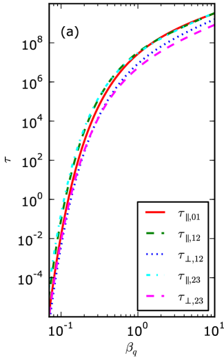
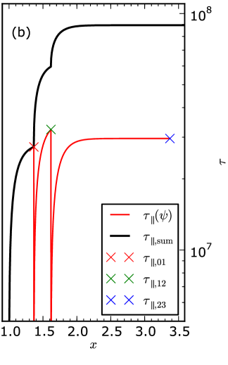
Figure 4.4: Panel (a) presents the dependence of the pair production optical depth on the magnetic field strength ($\beta_{q}=B/B_{q}$). Panel (b) presents the dependence of the optical depth on photon energy in the perpendicular frame of reference ($x=\epsilon\sin\Psi/\left(2mc^{2}\right)$). On both panels the photon energy is $\epsilon=500\,{\rm MeV}$, while panel (b) was obtained for magnetic field strength $\beta_{q}=1$.

4.2.4 Photon mean free path

As was shown in the previous section (see Figure 4.4) for strong magnetic fields (e.g. $\beta_{q}\gtrsim 0.2$), $\tau_{1}$, $\tau_{\|,2}$, and $\tau_{\perp,2}$ are much larger than one. Therefore, the pair production process takes place according to two scenarios (see also Medin and Lai,, 2010). If $\beta_{q}\gtrsim 0.2$ pairs are produced by photons almost immediately upon reaching the first threshold, the created pairs will be in the low Landau levels ($n\lesssim 2$). If $\beta_{q}\lesssim 0.2$, the photons will travel longer distances to be absorbed and the created pairs will be in the higher Landau levels.

Thus, for strong magnetic fields ($\beta_{q}\gtrsim 0.2$) the photon mean free path can be approximated as

$$l_{{\rm ph}}\approx s_{0}=\Re\frac{2mc^{2}}{E_{\gamma}},$$ (4.26)

while for relatively weak magnetic fields ($\beta_{q}\lesssim 0.2$) we can use the asymptotic approximation derived by Erber, (1966):

$$l_{{\rm ph}}\approx\frac{4.4}{(e^{2}/\hbar c)}\frac{\hbar}{mc}\frac{B_{q}}{B\sin\Psi}\exp\left(\frac{4}{3\chi}\right),$$ (4.27)

$$\chi\equiv\frac{E_{\gamma}}{2mc^{2}}\frac{B\sin\Psi}{B_{q}}\hskip 28.45274pt(\chi\ll 1).$$ (4.28)

4.2.5 Photon-splitting attenuation coefficient

In our calculations we include photon splitting by following the approach presented by Medin and Lai, (2010). Since only the $\perp\rightarrow\parallel\parallel$ process is allowed, for $\parallel$-polarised photons the photon splitting attenuation coefficient is zero $R_{\parallel}^{sp}=0$ (Adler,, 1971, Usov,, 2002, Baring and Harding,, 2001). To calculate the splitting attenuation coefficient in the perpendicular frame for $\perp$-polarised photons we use the formula adopted from the numerical calculation of Baring and Harding, (1997) :

$$R{}_{\perp}^{\prime{\rm sp}}\simeq\frac{\frac{\alpha_{f}^{2}}{60\pi^{2}}\left(\frac{26}{315}\right)^{2}\left(2x\right)^{5}\epsilon_{{\rm{}_{B}}}^{6}}{\left[\epsilon_{{}_{B}}^{3}\exp\left(-0.6x^{3}\right)+0.05\right]\left[0.25\epsilon_{{\rm{}_{B}}}^{3}\exp\left(-0.6x^{3}\right)+20\right]}.$$ (4.29)

For photon energies $x\leq 1$ this expression underestimates the results of Baring and Harding, (1997) at $\beta_{q}=1$ by less than $30\%$, while at both $\beta_{q}\leq 0.5$ and $\beta_{q}\gg 1$ the discrepancy is less than $10\%$. As can be seen from Figure 4.5, the attenuation coefficient $R{}_{\perp}^{\prime{\rm sp}}$ drops rapidly with the magnetic field strength for $\beta_{q}<1$, thus photon splitting is unimportant for $\beta_{q}\lesssim 0.5$ (e.g. Baring and Harding,, 2001; Medin and Lai,, 2010).

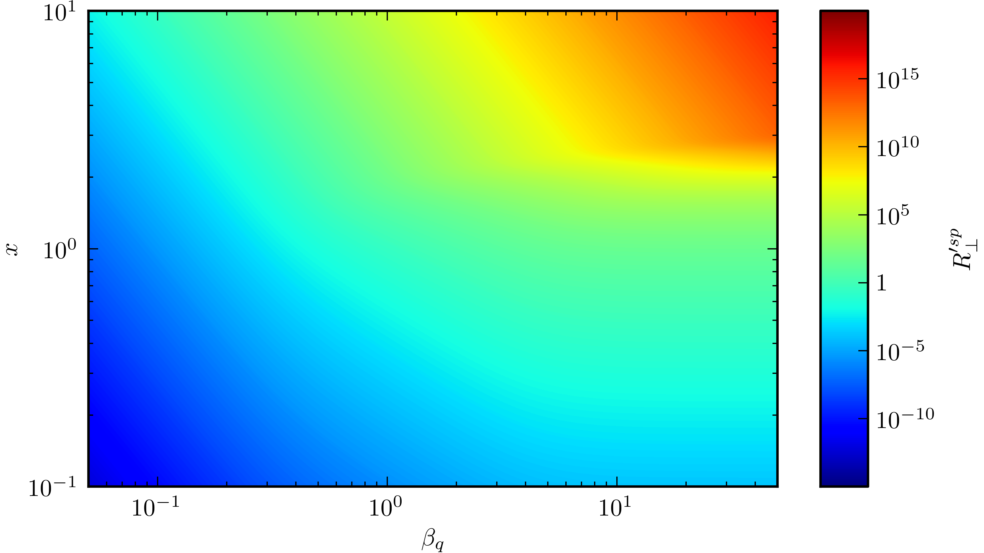
Figure 4.5: Dependence of the photon-splitting attenuation coefficient on the energy of the photon in the perpendicular frame ($x=\epsilon\sin\Psi/\left(2mc^{2}\right)$, vertical axis) and on the strength of the magnetic field ($\beta_{q}=B/B_{q}$, horizontal axis).

4.2.6 Pair creation vs photon splitting

As noted by Medin and Lai, (2010), even though the photon splitting attenuation coefficient above the first threshold ($x>x_{0}$) is much smaller than for pair production (see Figure 4.6), in ultrastrong magnetic fields ($\beta_{q}\gtrsim 0.5$) the $\perp$-polarised photons split before reaching the first threshold (see Figure 4.7). On the other hand, the $\parallel$-polarised photons produce pairs in the zeroth Landau level.

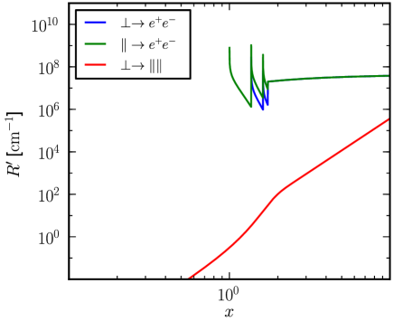
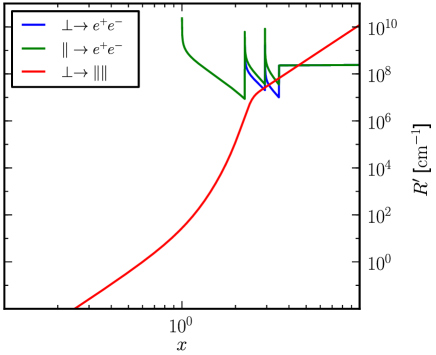
Figure 4.6: Attenuation coefficients of pair production and photon splitting in the perpendicular frame of reference. Panel (a) was obtained using photon energy $E_{\gamma}=10^{3}\,{\rm MeV}$ and magnetic field strength $B=B_{q}=4.414\times 10^{13}\,{\rm G}$ ($\beta_{q}=1$). Panel (b) presents calculations for photon energy $E_{\gamma}=10^{3}\,{\rm MeV}$ and magnetic field strength $B=2.5\times 10^{14}\,{\rm G}$ ($\beta_{q}=5.7$).

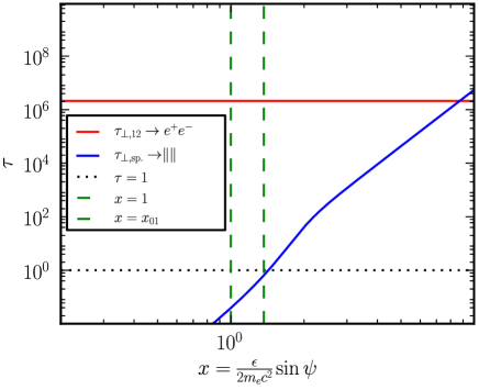
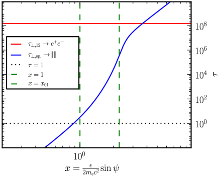
Figure 4.7: Optical depth for pair production and photon splitting for $\perp$-polarised photons. Panel (a) presents results for $E_{\gamma}=10^{3}\,{\rm MeV}$ and $B=B_{q}=4.4\times 10^{13}\,{\rm G}$ ($\beta_{q}=1$), while panel (b) was obtained using the same photon energy but a stronger magnetic field $B=2.5\times 10^{14}\,{\rm G}$ ($\beta_{q}=5.7$). If $\beta_{q}=1$ the photon creates an electron-positron pair, while in an ultrastrong magnetic field ($\beta_{q}=5.7$) the photon splits before it reaches the first threshold, $x=x_{0}$.

4.2.7 Secondary plasma

Following the approach presented by Medin and Lai, (2010) whenever $\tau\geq 1$ and the threshold for pair production is reached ($x=x_{0}$ for $\parallel$-polarised photons and $x=x_{1}$ for $\perp$-polarised photons), the photon is turned into an electron-positron pair. Whereas if $\tau_{{\rm sp}}\geq 1$ the photon is turned into two photons. Following the results of Baring and Harding,, 1997 we assume that the energy of parent photon is equally distributed between both newly created photons. A new $\parallel$-polarised photon is created with an energy $0.5\epsilon_{{\rm ph}}$ and weighting factor $2\Delta N_{\epsilon}$. We assume that the newly created photon travels in the same direction as the parent photon, ${\bf\Delta s_{ph}}$. Note that the photon should split with probability $1-e^{-\tau}$, but as shown by Medin and Lai, (2010) for cascade results this effect is negligible.

For $\beta_{q}\lesssim 0.1$, the particles are produced in high Landau levels with energy equal to half of the photon energy each (see Daugherty and Harding,, 1983). In our calculations we assume that the newly created particles (electron-positron pairs) travel in the same direction as the photon. When $\beta_{q}\gtrsim 0.1$, on the other hand, we choose the maximum allowed values of $j$ and $k$ for the newly created electron and positron. Note that for $\beta_{q}\gtrsim 0.1$ the particles are created in low Landau levels.

Figure 4.8 presents the spectrum of Curvature Radiation for a dipolar and non-dipolar structure of magnetic field lines. Note the characteristic three peaks in the CR distribution for the non-dipolar structure.

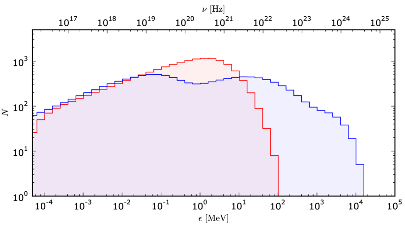
Figure 4.8: Distribution of CR photons produced by a single primary particle for a dipolar (blue line) and non-dipolar (red line) structure of the magnetic field. The minimum radius of curvature in thee dipolar case is $\Re_{6}^{{}^{{\rm min}}}\approx 50$, while in the non-dipolar case $\Re_{6}^{{}^{{\rm min}}}\approx 2$. In both cases the radiation was calculated up to a distance of $D=100R$, and with an initial Lorentz factor of the primary particle $\gamma_{{\rm c}}=3.5\times 10^{6}$.

Formation of the peaks is caused by the fact that the particle passes regions with three different values of curvature: (I) just above the stellar surface, $z\approx 1\,{\rm km}$, where curvature is the highest; (II) at altitudes where the influence of anomalies is comparable with the global dipole, $z\approx 2.5\,{\rm km}$, also with strong curvature; (III) and at altitudes where the influence of anomalies is negligible, $z\gtrsim 3.1R$, with approximately dipolar curvature (see Figure 2.11). Hence, the spectrum is a sum of radiation generated in a highly non-dipolar magnetic field (high energetic and soft $\gamma$-rays) and with radiation at higher altitudes where the magnetic field is dipolar (X-rays). The primary particle loses about $63\%$ and $1\%$ of its initial energy in the non-dipolar and dipolar case, respectively. As can be seen from the Figure, to get high emission of CR photons and, thus, a significant density of secondary plasma, a non-dipolar structure of the magnetic field is required.

The high energetic photons produced in a strongly non-dipolar magnetic field will either split or create electron-positron pairs. Figure 4.9 presents the distribution of particle energy created by CR photons. Note that for $\beta_{q}\lesssim 0.1$ the pairs are created in high Landau levels and in order to get the final distribution of secondary plasma energy we should consider the loss of particle energy due to Synchrotron Radiation (see Section 4.3).

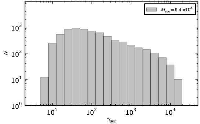
Figure 4.9: Distribution of particle energy created by CR photons calculated for a non-dipolar structure of the magnetic field. For this specific magnetic field configuration and initial parameters (see the caption of Figure 4.8) the secondary plasma multiplicity is $M_{{\rm sec}}\approx 6\times 10^{3}$. Note that this result does not include Synchrotron Radiation and the actual energies of the created pairs are lower as they lose their transverse momenta (see Section 4.3).

4.3 Synchrotron Radiation

When pairs (electrons and positrons) are created in high Landau Levels they radiate away their transverse momentum through Synchrotron Radiation (SR). The secondary positron (or electron) is created with energy $\gamma mc^{2}$ and pitch angle $\Psi$, which corresponds to a specific value of Landau Level $n$. Following Medin and Lai, (2010) we choose the frame in which the particle has no momentum along the direction of external magnetic field. In such a frame of reference the particle propagates in a circular motion transverse to the magnetic field (the so-called ”circular” frame). The relation of the energy of the newly created particle in the circular frame of reference ($E_{\perp}=\gamma_{\perp}mc^{2}$) with the particle energy in the co-rotating frame can be written as (Medin and Lai,, 2010)

$$\gamma_{\perp}=\sqrt{\gamma^{2}\sin^{2}\Psi+\cos^{2}\Psi}=\sqrt{1+2\epsilon_{{}_{B}}n}.$$ (4.30)

The power of synchrotron emission, $P_{{\rm SR}}$, can calculated as follows

$$P_{{\rm SR}}=\frac{2e^{2}}{3c^{3}}\left(\gamma_{\perp}^{2}-1\right)c^{2}\epsilon_{{}_{B}}^{2},$$ (4.31)

In the circular frame $E_{\perp}$, is radiated away through synchrotron emission after a particle travels a distance

$$l_{{\rm p}}^{{\rm SR}}\approx\left|\frac{E_{\perp}}{P_{{\rm SR}}}c\right|=\frac{\gamma_{\perp}mc^{3}}{\frac{2e^{2}}{3c^{3}}\left(\gamma_{\perp}^{2}-1\right)c^{2}\epsilon_{{\rm{}_{B}}}^{2}}.$$ (4.32)

The particle (electron or positron) mean free path for SR is much shorter than for other relevant cascade processes (see Section 4.1 for Curvature Radiation, and Section 4.4 for ICS). In fact, it is so short that in our calculations we assume that before moving from its initial position the particle loses all of its perpendicular momentum $p_{\perp}$ due to SR (see Daugherty and Harding,, 1982; Medin and Lai,, 2010). Once the particle reaches the ground Landau level ($n=0$, $p_{\perp}=0$) its final energy can be calculate as

$$\gamma_{\parallel}=\left(1-\beta^{2}\cos^{2}\Psi\right)^{-1/2}=\gamma/\gamma_{\perp},$$ (4.33)

here $\beta=v/c=\sqrt{1-1/\gamma^{2}}$ is the particle velocity in units of speed of light.

Following the approach presented by Medin and Lai, (2010), to simplify the simulation we assume that in the circular frame synchrotron photons are emitted isotropically in the plane of motion such that there is no perpendicular velocity change of the particle (the Lorentz factors $\gamma$ and $\gamma_{\perp}$ decrease but $\gamma_{\parallel}$ is constant). Thus, the Equation 4.33 remains valid until the particle reaches the ground state. In order to simulate the full SR process the following procedure was adopted: the particle Lorentz factor in the circular frame $\gamma_{\perp}$ drops from its initial value to $\gamma_{\perp}=1$ (i.e., $n=0$) in a series of steps. Each step entails emission of one synchrotron photon, with energy $\epsilon_{{}_{\perp}}$ depending on the current value of $\gamma_{\perp}$. After the photon emission the energy of the particle is reduced by $\epsilon_{{}_{\perp}}$, $\Delta\gamma_{\perp}=\epsilon_{{}_{\perp}}/mc^{2}$. Subsequently, the particle with reduced energy emits a photon with a new value of $\epsilon_{{}_{\perp}}$. This process continues until the particle is at $n=0$ Landau level. Depending on the particle’s Landau level $n$, the SR photon energy $\epsilon_{{}_{\perp}}$ is chosen in one of three ways.

(I) When the particle is created in a high Landau Level ($n\geq 3$), we choose the energy of the photon randomly but according to a probability based on the asymptotic synchrotron spectrum (e.g. Sokolov and Ternov, (1968), Harding and Preece, (1987)):

$$\frac{{\rm d}^{2}N}{{\rm d}t{\rm d}\epsilon_{\perp}}=\frac{\sqrt{3}}{2\pi}\frac{\alpha_{f}\epsilon_{{\rm{}_{B}}}}{\epsilon_{\perp}}\times\left[f\cdot F\left(\frac{\epsilon_{\perp}}{f\epsilon_{{\rm{}_{SR}}}}\right)+\left(\frac{\epsilon_{\perp}}{\gamma_{\perp}mc^{2}}\right)^{2}G\left(\frac{\epsilon_{{}_{\perp}}}{f\epsilon_{{\rm{}_{SR}}}}\right)\right],$$ (4.34)

where

$$\epsilon_{{}_{{\rm SR}}}=\frac{3}{2}\gamma_{\perp}^{2}\hbar\epsilon_{{}_{B}}$$ (4.35)

is the characteristic energy of the synchrotron photons, $f=1-\epsilon_{{}_{\perp}}/\left(\gamma_{\perp}mc^{2}\right)$ is the fraction of the electron’s energy after photon emission, $F\left(x\right)=x\int_{x}^{\infty}K_{5/3}\left(t\right){\rm d}t$, and $G\left(x\right)=xK_{2/3}\left(x\right)$. The functions $K_{5/3}$ and $K_{2/3}$ correspond to modified Bessel functions of the second kind. The expression in Equation 4.34 differs from the classical synchrotron spectrum (e.g. Rybicki and Lightman,, 1979) by a factor of $f=1-\epsilon_{{}_{\perp}}/\left(\gamma_{\perp}mc^{2}\right)$ which appears in several places in Equation 4.34 and by a term with the function $G\left(x\right)$. Note that in the classical expressions for the total radiation spectra these terms cancel out. However, as noted by Medin and Lai, (2010) when the quantum effects are considered there is asymmetry between the perpendicular and parallel polarisations such that term $G\left(x\right)$ remain.

(II) If $n=2$, the photon’s energy is either that required to lower the particle energy to its first excited state ($n=1$) or to the ground state ($n=0$). The probability of each process depends on the local magnetic field strength. We use the simplified prescription based on the results of Herold et al., (1982) to calculate the transition rates (see also Harding and Preece,, 1987). If $\beta_{q}<1$ the energy of the photon is set to lower the particle energy to the first excited state, $\epsilon_{{}_{\perp}}=mc^{2}\left(\sqrt{1+4\beta_{q}}-\sqrt{1+2\beta_{q}}\right)$. If $\beta_{q}\gtrsim 1$ the photon’s energy is randomly chosen to be that which is required to lower the particle energy to either the first excited state, or the ground state ($\epsilon_{\perp}=mc^{2}\left(\sqrt{1+4\beta_{q}}-1\right)$), with probability $50\%$ each.

(III) When $n=1$, the photon’s energy is chosen to lower the particle’s energy to its ground state, $\epsilon_{{}_{\perp}}=mc^{2}\left(\sqrt{1+2\beta_{q}}-1\right)$. If after emission of SR photon the particle is not in the ground state, $\gamma_{\perp}$ is recalculated and a new energy of photon is chosen.

The photon energy in the co-rotating frame can be calculated as

$$\epsilon=\gamma_{\parallel}\epsilon_{{}_{\perp}}.$$ (4.36)

The weighting factor of the emitted photon is the same as the secondary particle that emitted it ($\Delta N_{\epsilon}$ ). In the circular frame the photon is emitted in a random direction perpendicular to the magnetic field. Hence, in the co-rotating frame the emission angle can be calculated using Equations 4.30 and 4.33 as follows

$$\Psi=\arcsin\sqrt{\frac{\gamma_{\perp}^{2}-1}{\gamma_{\perp}^{2}\gamma_{\parallel}^{2}-1}}\cos\Pi,$$ (4.37)

where $\Pi$ is a random number from $0$ to $2\pi$. In our simulation we include this emission angle by using the same approach as presented in Section 4.2.1, but as the maximum value we use $\Psi$ instead of $1/\gamma$.

The polarisation fraction of SR photons is the exact opposite of the CR case and it ranges from $50\%$ to $100\%$ polarised perpendicular to the magnetic field. Following the approach presented by Medin and Lai, (2010) in our calculations the photon polarisation is randomly assign in the ratio of one $\parallel$ to every seven $\perp$ photons, which corresponds to a $75\%$ perpendicular polarisation.

Figure 4.10 presents the distribution of SR produced by a single secondary particle. To show the nature of the distribution, a relatively high pitch angle was used. Note that when a particle is created at a distance where the magnetic field is relatively weak (e.g. $\beta_{q}=10^{-5}$ for $\gamma=10^{2}$) then most of the energy is radiated in the range of $1-10\,{\rm keV}$. Thus, we believe that if a strong enough instability forms (that increases the particle’s pitch angle), the SR process could be responsible for the production of a non-thermal component of the X-ray spectrum.

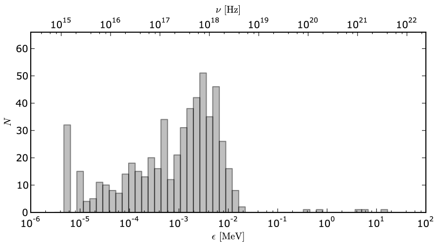
Figure 4.10: Distribution of SR produced by a single secondary particle with Lorentz factor $\gamma=10^{2}$. We have assumed that the particle was created in a region where the magnetic field strength was $B=4.14\times 10^{8}$ ($\beta_{q}=10^{-5}$) and with a pitch angle $\Psi=7^{\circ}$. For such a relatively high pitch angle the particle loses most of its energy ending with Lorentz factor $\gamma_{{\rm end}}\approx 6$.

Figure 4.11 presents the final spectrum produced by a single primary particle with an initial Lorentz factor of $\gamma_{{\rm c}}=3.5\times 10^{6}$ for a non-dipolar configuration of the surface magnetic field of PSR J0633+1746 (see Section 2.4.2). Due to CR the particle loses about $68\%$ of its initial energy ($\Delta\epsilon=2.2\times 10^{6}mc^{2}$), which is radiated mainly in close vicinity of a neutron star, where curvature of the magnetic field is the highest. As the $\gamma$-photons propagate they will split (only if the magnetic field is strong enough) and eventually most photons will be absorbed by the magnetic field - as a result electron-positron pairs emerge. These pairs radiate away their transverse momenta through SR, producing mainly X-ray photons (at larger distances) and only a few $\gamma$-photons (in a strong magnetic field just above the stellar surface). Note that at the end (after pair production) only $14\%$ of the primary particle’s energy ($\Delta\epsilon_{{\rm ph}}=4\times 10^{5}mc^{2}$) is converted into photons and the bulk of its energy, $54\%$ ($\Delta\epsilon_{{\rm pairs}}=1.8\times 10^{6}mc^{2}$), is allocated into secondary plasma. The multiplicity for this specific simulation is of the order $M_{{\rm sec}}=10^{4}$. Note that we use $M_{{\rm sec}}$ to describe the multiplicity of secondary plasma in contrast to $M_{{\rm pr}}$ which describes particle multiplicity in the IAR.

Figure 4.11: Final photon distribution produced by a single primary particle. The blue line corresponds to the initial CR photons distribution for a non-dipolar structure of the magnetic field, while the red line presents the final distribution with the inclusion of photon splitting, pair production and SR.

Figure 4.12 presents the distribution of particle energy created by CR photons but with the inclusion of SR emission (red line). Note that synchrotron emission both lowers the particle energy (after SR maximum at $\gamma\approx 5-8$, while without SR at $\gamma\approx 15-20$) and increases the multiplicity of secondary plasma $M_{{\rm sec}}\approx 10^{4}$.

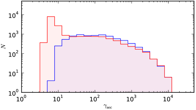
Figure 4.12: Distribution of particle energy created by CR photons calculated for a non-dipolar structure of the magnetic field. For this specific magnetic field configuration and initial parameters (see the caption of Figure 4.8) the secondary plasma multiplicity is $M_{{\rm sec}}\approx 10^{4}$. Note that this result does not include Synchrotron Radiation and the actual energies of the created pairs are lower as they lose their transverse momenta (see Section 4.3).

4.4 Inverse Compton Scattering

The Inverse Compton Scattering (hereafter ICS) process in the neutron star vicinity has been studied extensively by Xia, (1982); Kardashëv et al., (1984); Xia et al., (1985); Daugherty and Harding, (1989); Dermer, (1989, 1990); Bednarek et al., (1992); Chang, (1995); Sturner, (1995); Zhang and Qiao, (1996); Zhang et al., (1997); Zhang and Harding, (2000); Harding et al., (2002), etc. According to these studies, the ICS process may play a significant role in the physics of a neutron star’s magnetosphere. Relativistic particles (positrons and electrons) can Compton-scatter thermal radiation from the neutron star surface. As a particle with a certain relativistic velocity scatters the thermal photons with a blackbody distribution, it will produce radiation in quite a wide energy range. However, we can distinguish two characteristic frequencies of upscattered photons: one is the frequency due to resonant scattering, another is the range of frequencies contributed by the scattering of photons with frequencies around the ”thermal-peak”. The Resonant Inverse Compton Scattering (RICS) corresponds to a scenario when the scattering cross section is largest. On the other hand, Thermal-peak Inverse Compton Scattering (TICS) corresponds to interactions with photons with the maximum number density. These two modes are very different when it comes to the nature of the process. The photons’ energy in RICS depends on the strength of the magnetic field, thus at low altitudes (where the field is very strong), it can power pair cascades, while TICS can be responsible for magnetospheric radiation at much higher altitudes. Note that for some specific combinations of magnetic strength and distribution of background photons, RICS and TICS are indistinguishable as the resonance frequency falls into the thermal peak range.

4.4.1 The cross section of ICS

Due to the rapid time scale for synchrotron emission (see section 4.3), a particle in an excited Landau level almost instantaneously de-excites to the ground level. The particle motion is therefore strongly confined to the magnetic field direction. In our calculations we consider the geometry illustrated in Figure 4.13. In the observer’s frame of reference (OF), a particle with Lorentz factor $\gamma$ travelling along the magnetic field line scatters a photon. Let $\psi=\arccos\mu$ be the angle between the magnetic field line (particle propagation) and the direction of photon propagation in OF and $\psi^{\prime}=\arccos\mu^{\prime}$ in the particle rest frame (PRF). The energy of the photon in PRF is given by

$$\epsilon^{\prime}=\gamma\epsilon\left(1-\beta\mu\right).$$ (4.38)

After scattering, the photon energy is denoted by $\epsilon{}_{s}^{\prime}$ in PRF and $\epsilon_{s}$ in OF. The angle between the direction of propagation of the scattered photon and ${\bf B}$ (which describes the direction of particle propagation) is denoted by $\psi_{s}=\arccos\mu_{s}$ in OF and $\psi{}_{s}^{\prime}=\arccos\mu{}_{s}^{\prime}$, where $\mu{}_{s}^{\prime}=\left(\mu_{s}-\beta\right)/\left(1-\beta\mu_{s}\right)$ in PRF (Dermer,, 1990).

Figure 4.13: Reproduction of the Figure from Dermer, (1990). Geometry of the ICS event in the observer’s frame (left) and the particle rest frame (right). A particle with Lorentz factor $\gamma$, beamed along the direction of the magnetic field, scatters a photon with energy $\epsilon$ directed at angle $\psi$ with respect to the magnetic field line. After scattering, the energy and angle of the photon are denoted by $\epsilon_{s}$ and $\psi_{s}$, respectively. Quantities in the particle rest frame are denoted by a prime.

4.4.1.1 ICS cross section in the Thomson regime

Restriction to the Thomson regime requires that $\gamma\epsilon\left(1-\mu\right)\ll 1$. In the particle rest frame, the angle $\psi^{\prime}=\arcsin\left\{\gamma^{-1}\left[\sin\psi/\left(1-\beta\cos\psi\right)\right]\right\}$, and when $\gamma\gg 1$, $\left|\mu^{\prime}\right|\to 1$. In the Thomson regime the only important Compton scattering process involves transitions between ground-state Landau levels. Daugherty and Harding, (1989) and Dermer, (1989) calculated the differential cross section (after summing over polarisation modes and integrating over azimuth) for a photon scattered from $\psi^{\prime}=0^{\circ}$ into angle $\psi{}_{s}^{\prime}=\arccos\mu{}_{s}^{\prime}$ as follows

$$\frac{{\rm d}\sigma^{\prime}}{{\rm d}\mu{}_{s}^{\prime}}=\frac{3\sigma_{{}_{{\rm T}}}}{16}\left(1+\mu{}_{s}^{\prime 2}\right)\left[\frac{\epsilon{}^{\prime 2}}{\left(\epsilon^{\prime}+\epsilon_{{}_{B}}\right){}^{2}}+\frac{\epsilon{}^{\prime 2}}{\left(\epsilon^{\prime}-\epsilon_{{}_{B}}\right){}^{2}+\left(\Gamma/2\right){}^{2}}\right],$$ (4.39)

where $\Gamma=4\alpha_{f}\epsilon_{{}_{B}}^{2}/3$ is the resonant width (Daugherty and Ventura,, 1978; Xia et al.,, 1985), $\sigma_{{}_{{\rm T}}}$ is the Thomson cross section, and $\alpha_{f}=e^{2}/\hbar c$ is the fine-structure constant. In the Thomson limit $\epsilon^{\prime}\ll 1$, and thus the scattered photon energy in PRF can be approximated as

$$\epsilon{}_{s}^{\prime}\simeq\epsilon^{\prime}+\epsilon{}^{\prime 2}(\mu^{\prime}-\mu{}_{s}^{\prime})^{2}/2\approx\epsilon^{\prime}.$$ (4.40)

Equations 4.39 and 4.40 show that a differential magnetic Compton scattering cross section when $\gamma\gg 1$ is similar in form to a nonmagnetic Thomson cross section. The important difference is that the magnitude of the cross section is enhanced when $\epsilon^{\prime}$ approaches $\epsilon_{{}_{B}}$ and is depressed at energies $\epsilon^{\prime}<\epsilon_{{}_{B}}$. The total cross section for magnetic Compton scattering, obtained by integrating Equation 4.39 over $\mu{}_{s}^{\prime}$, was calculated by Dermer, (1989); Zhang et al., (1997) and is given by

$$\sigma^{\prime}=\frac{\sigma_{{}_{{\rm IC}}}}{2}\left[\frac{u^{2}}{\left(u+1\right){}^{2}}+\frac{u^{2}}{\left(u-1\right){}^{2}+a^{2}}\right],$$ (4.41)

where $\sigma_{{}_{{\rm IC}}}=\sigma_{{\rm{}_{T}}}$, $\sigma_{{\rm{}_{T}}}$ is the Thomson cross section, $u=\epsilon^{\prime}/\epsilon_{{}_{B}}$, $a=\frac{2}{3}\alpha_{f}\epsilon_{{}_{B}}$.

4.4.1.2 ICS cross section in the Klein-Nishina regime

The Klein-Nishina regime includes quantum effects due to the relativistic nature of scattering, and it requires that $\gamma\epsilon\left(1-\mu\right)\gtrsim 1$. The principal effect is to reduce the cross section from its classical value as the photon energy in PRF becomes large. In the Klein-Nishina regime instead of $\sigma_{{\rm{}_{IC}}}=\sigma_{{}_{{\rm T}}}$ we can use the following relationship

$$\sigma_{{}_{{\rm IC}}}=\sigma_{{}_{{\rm KN}}}=\frac{3}{4}\sigma_{{}_{{\rm T}}}\left\{\frac{1+\epsilon^{\prime}}{\epsilon^{\prime 3}}\left[\frac{2\epsilon^{\prime}\left(1+\epsilon^{\prime}\right)}{1+2\epsilon^{\prime}}-\ln\left(1+2\epsilon^{\prime}\right)\right]+\frac{1}{2\epsilon^{\prime}}\ln\left(1+2\epsilon^{\prime}\right)-\frac{1+3\epsilon^{\prime}}{\left(1+2\epsilon^{\prime}\right)^{2}}\right\}.$$ (4.42)

In an extreme relativistic regime $\epsilon^{\prime}\gg 1$ the Klein-Nishina formula can be simplified to

$$\sigma_{{\rm{}_{KN}}}\approx\frac{3}{8}\sigma_{{}_{{\rm T}}}\epsilon^{\prime-1}\left[\ln\left(2\epsilon^{\prime}\right)+\frac{1}{2}\right].$$ (4.43)

The above formula clearly shows that Inverse Compton Scattering is less efficient for photons with energy in PRF significantly exceeding particle rest energy.

4.4.1.3 QED Compton Scattering cross section

Previous studies on upscattering and energy loss by relativistic particles have used the non-relativistic, magnetic Thomson cross section for resonant scattering or the Klein-Nishina cross section for thermal-peak scattering. As noted by Gonthier et al., (2000), this approach does not account for the relativistic quantum effects of strong magnetic fields ($B>10^{12}\,{\rm G}$). When the photon energy exceeds $mc^{2}$ in the particle rest frame, the strong magnetic field significantly lowers the Compton scattering cross section below and at the resonance. Gonthier et al., (2000) developed expressions for the scattering of ultrarelativistic electrons with $\gamma\gg 1$ moving parallel to the magnetic field. Because of the large Lorentz Factor of particle $\gamma$, the photon incident angle $\psi$ gets Lorentz concentrated to $\psi^{\prime}\approx\psi/2\gamma\approx 0^{\circ}$ in the PRF. The differential cross section in the rest frame of the particle can be written as

$$\frac{{\rm d}\sigma{}_{\|,\perp}^{\prime}}{{\rm d}\cos\psi{}_{s}^{\prime}}=\frac{3\sigma_{{}_{{\rm T}}}}{16\pi}\frac{\epsilon{}_{s}^{\prime 2}e^{-\epsilon{}_{s}^{\prime 2}\sin^{2}\left(\psi_{s}^{\prime}/2\epsilon_{{}_{B}}\right)}}{\epsilon^{\prime}\left(2+\epsilon^{\prime}-\epsilon{}_{s}^{\prime}\right)\left[\epsilon{}_{s}^{\prime}+\epsilon^{\prime}\epsilon{}_{s}^{\prime}\left(1-\cos\psi{}_{s}^{\prime}\right)-\epsilon{}_{s}^{\prime 2}\sin^{2}\psi{}_{s}^{\prime}\right]}\frac{1}{l!}\left(\frac{\epsilon{}_{s}^{\prime 2}\sin^{2}\psi{}_{s}^{\prime}}{2\epsilon_{{}_{B}}}\right)G_{\|,\perp},$$ (4.44)

where

$$G_{\|}=\hat{G}_{\mathrm{no-flip}}^{\|}+\hat{G}_{\mathrm{flip}}^{\|},\hskip 28.45274ptG_{\perp}=\hat{G}_{\mathrm{no-flip}}^{\perp}+\hat{G}_{\mathrm{flip}}^{\perp}$$ (4.45)

and

$$\begin{split}\hat{G}_{\mathrm{no-flip}}^{\|}=&\int_{0}^{2\pi}\left|G_{\mathrm{no-flip}}^{\|,\|}\right|^{2}{\rm d}\phi^{\prime}=\int_{0}^{2\pi}\left|G_{\mathrm{no-flip}}^{\perp,\|}\right|^{2}{\rm d}\phi^{\prime}=\\ =&2\pi\left\{\left[\left(B_{1}+B_{3}+B_{7}\right)\cos\psi{}_{s}^{\prime}-\left(B_{2}+B_{6}\right)\sin\psi{}_{s}^{\prime}\right]^{2}+\left(B_{4}\cos\psi{}_{s}^{\prime}-B_{5}\sin\psi{}_{s}^{\prime}\right)^{2}\right\},\\ \hat{G}_{\mathrm{no-flip}}^{\perp}=&\int_{0}^{2\pi}\left|G_{\mathrm{no-flip}}^{\|,\perp}\right|^{2}{\rm d}\phi^{\prime}=\int_{0}^{2\pi}\left|G_{\mathrm{no-flip}}^{\perp,\perp}\right|^{2}{\rm d}\phi^{\prime}=\\ =&2\pi\left[\left(B_{1}-B_{3}-B_{7}\right)^{2}+B_{4}^{2}\right],\\ \hat{G}_{\mathrm{flip}}^{\|}=&\int_{0}^{2\pi}\left|G_{\mathrm{flip}}^{\|,\|}\right|^{2}{\rm d}\phi^{\prime}=\int_{0}^{2\pi}\left|G_{\mathrm{flip}}^{\perp,\|}\right|^{2}{\rm d}\phi^{\prime}=\\ =&2\pi\left\{\left[\left(C_{1}+C_{3}+C_{7}\right)\cos\psi{}_{s}^{\prime}-\left(C_{2}+C_{6}\right)\sin\psi{}_{s}^{\prime}\right]^{2}+\left(C_{4}\cos\psi{}_{s}^{\prime}-C_{5}\sin\psi{}_{s}^{\prime}\right)^{2}\right\},\\ \hat{G}_{\mathrm{flip}}^{\perp}=&\int_{0}^{2\pi}\left|G_{\mathrm{flip}}^{\|,\perp}\right|^{2}{\rm d}\phi^{\prime}=\int_{0}^{2\pi}\left|G_{\mathrm{flip}}^{\perp,\perp}\right|^{2}{\rm d}\phi^{\prime}=\\ =&2\pi\left[\left(C_{1}-C_{3}-C_{7}\right)^{2}+C_{4}^{2}\right].\end{split}$$ (4.46)

The imaginary terms and the $\phi^{\prime}$ dependence are isolated in the polarisation components and in the phase exponentials, leading to elementary integrations over the azimuthal angle, $\phi^{\prime}$ (Gonthier et al.,, 2000).

The differential cross section depends on the final Landau state $l$, thus a sum must be calculated over all the contributing Landau states. The energy of the scattered photon is given by (Gonthier et al.,, 2000)

$$\epsilon{}_{s}^{\prime}=\frac{2\left(\epsilon^{\prime}-l\epsilon_{{}_{B}}\right)}{1+\epsilon^{\prime}\left(1-\cos\psi{}_{s}^{\prime}\right)+\left\{\left[1+\epsilon^{\prime}\left(1-\cos\psi{}_{s}^{\prime}\right)\right]^{2}-2\left(\epsilon^{\prime}-l\epsilon_{{}_{B}}\right)\sin^{2}\psi{}_{s}^{\prime}\right\}^{\frac{1}{2}}},$$ (4.47)

where $l$ is the final Landau level of the scattered particle. Each final state has an energy threshold of $l\epsilon_{{}_{B}}$, thus the maximum contributing Landau state $l_{{\rm max}}$ can be expressed as: $\epsilon^{\prime}/\epsilon_{{}_{B}}-1<l_{{\rm max}}<\epsilon^{\prime}/\epsilon_{{}_{B}}$. To obtain the energy-dependent cross section, the Romberg’s method can be used to numerically integrate the differential cross section over $\psi{}_{s}^{\prime}$. For this particular case (scattering of relativistic particles) there is only one resonance appearing at the fundamental cyclotron frequency $\epsilon_{{}_{B}}=\beta_{q}=eB/\left(mc\right)$.

The values of $B$ and $C$ can be expressed as:

$$\begin{split}B_{1}=&\frac{2\epsilon^{\prime}-\epsilon^{\prime}\epsilon{}_{s}^{\prime}\left(1-\cos\psi{}_{s}^{\prime}\right)}{2\left(\epsilon^{\prime}-\epsilon_{{}_{B}}\right)},\\ B_{2}=&-\frac{\left(\epsilon^{\prime}-\epsilon{}_{s}^{\prime}\cos\psi{}_{s}^{\prime}\right)\left(2l\epsilon_{{}_{B}}-\epsilon{}_{s}^{\prime 2}\sin^{2}\psi{}_{s}^{\prime}\right)+2l\epsilon_{{}_{B}}\epsilon^{\prime}}{2\epsilon{}_{s}^{\prime}\sin\psi{}_{s}^{\prime}\left(\epsilon^{\prime}-\epsilon_{{}_{B}}\right)},\\ B_{3}=&\frac{l\epsilon_{{}_{B}}\left(2l\epsilon_{{}_{B}}-2\epsilon_{{}_{B}}-\epsilon{}_{s}^{\prime 2}\sin^{2}\psi{}_{s}^{\prime}\right)}{\epsilon{}_{s}^{\prime 2}\sin^{2}\left[\psi{}_{s}^{\prime}\left(\epsilon^{\prime}-\epsilon_{{}_{B}}\right)\right]},\\ B_{4}=&-\frac{2\epsilon{}_{s}^{\prime}+\epsilon^{\prime}\epsilon{}_{s}^{\prime}\left(1-\cos\psi{}_{s}^{\prime}\right)-\epsilon{}_{s}^{\prime 2}\sin^{2}\psi{}_{s}^{\prime}}{2\left[\epsilon^{\prime}\epsilon{}_{s}^{\prime}\left(1-\cos\psi{}_{s}^{\prime}\right)-\epsilon^{\prime}-\epsilon_{{}_{B}}\right]},\\ B_{5}=&-\frac{\left(\epsilon^{\prime}-\epsilon{}_{s}^{\prime}\cos\psi{}_{s}^{\prime}\right)\epsilon{}_{s}^{\prime}\sin\psi{}_{s}^{\prime}}{2\left[\epsilon^{\prime}\epsilon{}_{s}^{\prime}\left(1-\cos\psi{}_{s}^{\prime}\right)-\epsilon^{\prime}-\epsilon_{{}_{B}}\right]},\\ B_{6}=&\frac{l\epsilon_{{}_{B}}\cos\psi{}_{s}^{\prime}}{\sin\psi{}_{s}^{\prime}\left[\epsilon^{\prime}\epsilon{}_{s}^{\prime}\left(1-\cos\psi_{s}^{\prime}\right)-\epsilon^{\prime}+\epsilon_{{}_{B}}\right]},\\ B_{7}=&\frac{2l\left(l-1\right)\epsilon_{{}_{B}}^{2}}{\epsilon{}_{s}^{\prime 2}\sin^{2}\psi{}_{s}^{\prime}\left[\epsilon^{\prime}\epsilon{}_{s}^{\prime}\left(1-\cos\psi{}_{s}^{\prime}\right)-\epsilon^{\prime}+\epsilon_{{}_{B}}\right]},\\ C_{1}=&\sqrt{2l\epsilon_{{}_{B}}}\frac{\epsilon^{\prime}}{2\left(\epsilon^{\prime}-\epsilon_{{}_{B}}\right)},\\ C_{2}=&-\sqrt{2l\epsilon_{{}_{B}}}\frac{2\epsilon^{\prime}+2\epsilon^{\prime}{}^{2}-\epsilon^{\prime}\epsilon{}_{s}^{\prime}\left(1-\cos\psi{}_{s}^{\prime}\right)-2l\epsilon_{{}_{B}}+\epsilon{}_{s}^{\prime 2}\sin^{2}\psi{}_{s}^{\prime}}{2\epsilon^{\prime}{}_{s}\sin\psi{}_{s}^{\prime}\left(\epsilon^{\prime}-\epsilon_{{}_{B}}\right)},\\ C_{3}=&\sqrt{2l\epsilon_{{}_{B}}}\frac{\left(\epsilon^{\prime}-\epsilon_{s}^{\prime}\cos\psi{}_{s}^{\prime}\right)\left(2l\epsilon_{{}_{B}}-2\epsilon_{{}_{B}}-\epsilon{}_{s}^{\prime 2}\sin^{2}\psi{}_{s}^{\prime}\right)}{2\epsilon{}_{s}^{\prime 2}\sin^{2}\psi{}_{s}^{\prime}\left(\epsilon^{\prime}-\epsilon_{{}_{B}}\right)},\\ C_{4}=&-\sqrt{2l\epsilon_{{}_{B}}}\frac{\epsilon{}_{s}^{\prime}\cos\psi{}_{s}^{\prime}}{2\left[\epsilon{}_{s}^{\prime}\epsilon^{\prime}\left(1-\cos\psi{}_{s}^{\prime}\right)-\epsilon^{\prime}-\epsilon_{{}_{B}}\right]},\\ C_{5}=&\sqrt{2l\epsilon_{{}_{B}}}\frac{\epsilon{}_{s}^{\prime}\sin\psi{}_{s}^{\prime}}{2\left[\epsilon{}_{s}^{\prime}\epsilon^{\prime}\left(1-\cos\psi{}_{s}^{\prime}\right)-\epsilon^{\prime}-\epsilon_{{}_{B}}\right]},\\ C_{6}=&-\sqrt{2l\epsilon_{{}_{B}}}\frac{2\epsilon{}_{s}^{\prime}+\epsilon^{\prime}\epsilon{}_{s}^{\prime}\left(1-\cos\psi{}_{s}^{\prime}\right)-\epsilon{}_{s}^{\prime 2}\sin^{2}\psi{}_{s}^{\prime}}{2\epsilon{}_{s}^{\prime}\sin\psi{}_{s}^{\prime}\left[\epsilon{}_{s}^{\prime}\epsilon^{\prime}\left(1-\cos\psi{}_{s}^{\prime}\right)-\epsilon^{\prime}+\epsilon_{{}_{B}}\right]},\\ C_{7}=&\sqrt{2l\epsilon_{{}_{B}}}\frac{\left(l-1\right)\epsilon_{{}_{B}}\left(\epsilon^{\prime}-\epsilon{}_{s}^{\prime}\cos\psi{}_{s}^{\prime}\right)}{\epsilon{}_{s}^{\prime 2}\sin^{2}\psi{}_{s}^{\prime}\left[\epsilon{}_{s}^{\prime}\epsilon^{\prime}\left(1-\cos\psi{}_{s}^{\prime}\right)-\epsilon^{\prime}+\epsilon_{{}_{B}}\right]}.\end{split}$$ (4.48)

Although the expressions presented above describe the exact cross section for ICS in strong magnetic fields, due to their complexity their usage in cascade simulation is limited.

4.4.1.4 Approximate cross section (final states l=0)

An approximation to the exact $l=0$ differential cross section can be given by assuming that the scattering is significantly below the resonance, where $\epsilon^{\prime}<\epsilon_{{}_{B}}$ and also $\epsilon^{\prime}<1$. Gonthier et al., (2000) showed that by keeping only terms to first order in $\epsilon^{\prime}$ and $\epsilon{}_{s}^{\prime}$ in the region of validity, it agrees very well with the exact $l=0$ cross section. The approximation overestimates the exact $l=0$ cross section above the region of validity $\epsilon^{\prime}>\epsilon_{{}_{B}}$. However, the approximation is close to the total cross section for both energy regions ($\epsilon^{\prime}<\epsilon_{{}_{B}}$ and $\epsilon^{\prime}>\epsilon_{{}_{B}}$ ), even for high magnetic field strengths (see Figure 4.14).

According to Gonthier et al., (2000), the polarisation-dependent and averaged, approximate cross section can be calculated as:

$$\sigma{}^{\prime\|\rightarrow\|}=\sigma{}^{\prime\perp\rightarrow\|}=\frac{3\sigma_{{}_{{\rm T}}}}{16}\left[g\left(\epsilon^{\prime}\right)-h\left(\epsilon^{\prime}\right)\right]\left[\frac{1}{\left(\epsilon^{\prime}-\epsilon_{{}_{B}}\right)^{2}}+\frac{1}{\left(\epsilon^{\prime}+\epsilon_{{}_{B}}\right)^{2}}\right],$$ (4.49)

$$\sigma{}^{\prime\|\rightarrow\perp}=\sigma{}^{\prime\perp\rightarrow\perp}=\frac{3\sigma_{{}_{{\rm T}}}}{16}\left[f\left(\epsilon^{\prime}\right)-2\epsilon^{\prime}h\left(\epsilon^{\prime}\right)\right]\left[\frac{1}{\left(\epsilon^{\prime}-\epsilon_{{}_{B}}\right)^{2}}+\frac{1}{\left(\epsilon^{\prime}+\epsilon_{{}_{B}}\right)^{2}}\right],$$ (4.50)

$$\sigma{}_{{\rm avg}}^{\prime}=\frac{3\sigma_{{}_{{\rm T}}}}{16}\left[g\left(\epsilon^{\prime}\right)+f\left(\epsilon^{\prime}\right)-\left(1+2\epsilon^{\prime}\right)h\left(\epsilon^{\prime}\right)\right]\left[\frac{1}{\left(\epsilon^{\prime}-\epsilon_{{}_{B}}\right)^{2}}+\frac{1}{\left(\epsilon^{\prime}+\epsilon_{{}_{B}}\right)^{2}}\right],$$ (4.51)

$$\begin{array}[]{c}g\left(\epsilon^{\prime}\right)=\frac{\epsilon^{\prime 2}\left(3+2\epsilon^{\prime}\right)+2\epsilon^{\prime}}{\sqrt{\epsilon^{\prime}\left(2+\epsilon^{\prime}\right)}}\ln\left[1+\epsilon^{\prime}-\sqrt{\epsilon^{\prime}\left(2+\epsilon^{\prime}\right)}\right]+\frac{\epsilon^{\prime}}{2}\ln\left(1+4\epsilon^{\prime}\right)+\\ +\epsilon^{\prime}\left(1+2\epsilon^{\prime}\right)\ln\left(1+2\epsilon^{\prime}\right)+2\epsilon^{\prime},\end{array}$$ (4.52)

$$f\left(\epsilon^{\prime}\right)=-\epsilon{}^{\prime 2}\ln\left(1+4\epsilon^{\prime}\right)+\epsilon^{\prime}\left(1+2\epsilon^{\prime}\right)\ln\left(1+2\epsilon^{\prime}\right),$$ (4.53)

$$h\left(\epsilon^{\prime}\right)=\left\{\begin{array}[]{ll}\frac{\epsilon{}^{\prime 2}}{\sqrt{\epsilon^{\prime}\left(2-\epsilon^{\prime}\right)}}\arctan\left[\frac{\sqrt{\epsilon^{\prime}\left(2-\epsilon^{\prime}\right)}}{1+\epsilon^{\prime}}\right]&\mbox{ for $\epsilon^{\prime}<2$},\\ \frac{\epsilon^{\prime}{}^{2}}{2\sqrt{\epsilon^{\prime}\left(\epsilon^{\prime}-2\right)}}\ln\left[\frac{\left(1+\epsilon^{\prime}+\sqrt{\epsilon^{\prime}(\epsilon^{\prime}-2)}\right)^{2}}{1+4\epsilon^{\prime}}\right]&\mbox{ for $\epsilon^{\prime}>2$}.\end{array}\right.$$ (4.54)

Figure 4.14 presents the total approximate cross section of Compton scattering, the exact QED cross section (summed over all contributing final electron/positron Landau states) and the exact cross section for final Landau state $l=0$ as a function of energy of the incident photon in PRF (in units of cyclotron energy, $\epsilon^{\prime}/\epsilon_{{}_{B}}$). As mentioned above, the approximation is valid in the region below the resonance, $\epsilon^{\prime}<\epsilon_{{}_{B}}$. Although the approximation overestimates the cross section for $l=0$ final Landau state in the regime of high energetic photons ($\epsilon^{\prime}>\epsilon_{{}_{B}}$), it can be used in this regime as the approximation of the total cross section. In our simulation we use this approach to calculate the total ICS cross section in both regimes, $\epsilon^{\prime}<\epsilon_{{}_{B}}$ and $\epsilon^{\prime}>\epsilon_{{}_{B}}$. Calculation of the cross section for the resonance frequency ($\epsilon^{\prime}=\epsilon_{{\rm{}_{B}}}$) is presented in the next section.

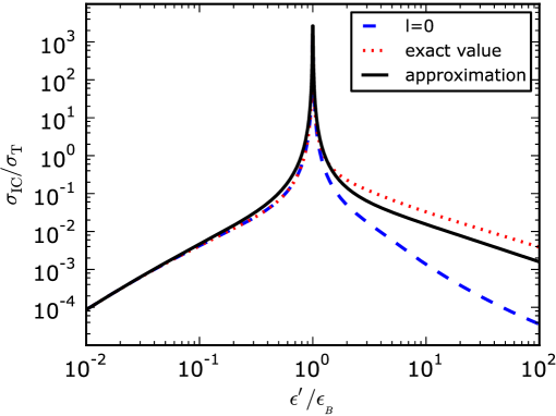
Figure 4.14: Total cross section of Compton scattering (in Thomson units) as a function of an incident photon energy in PRF (in units of the cyclotron energy) calculated for a magnetic field strength $B_{14}=3.5$. The exact QED scattering cross section, summed over all contributing final electron/positron Landau states, is indicated as the red dotted curve. The cross section for final Landau states $l=0$ is plotted as a blue dashed line.

4.4.2 Resonant Compton Scattering

This section describes an approach used to calculate the RICS cross section for ultrastrong magnetic fields ($B>10^{12}\,{\rm G}$). For weaker fields the calculations are much simpler and resonance is already included in Equation 4.41.

The trend as $\beta_{q}$ increases is for the magnitude of the cross section to drop at all energies. For weaker magnetic fields ($\beta_{q}<1$) the width of the resonance increases with increasing $\beta_{q}$, but for $\beta_{q}\geq 1$ this width actually declines. Since the resonance is formally divergent, the common practice (see Xia et al.,, 1985; Latal,, 1986; Daugherty and Harding,, 1989; Dermer,, 1990; Harding and Daugherty,, 1991; Baring et al.,, 2005; Harding and Lai,, 2006; Baring and Harding,, 2007, 2008) is to truncate it at $\epsilon^{\prime}=\epsilon_{{}_{B}}$ by introducing a finite width $\Gamma$. The procedure is to replace the resonant $\left(\epsilon^{\prime}-\epsilon_{{}_{B}}\right)^{2}$ denominator (see Equations 4.44 and 4.51) by $\left[\left(\epsilon^{\prime}-\epsilon_{{}_{B}}\right)^{2}+\Gamma^{2}/4\right]$. In the $\beta_{q}\ll 1$ regime, the cyclotron decay width assumes the well-known result $\Gamma\approx 4\alpha_{f}\epsilon_{{}_{B}}^{2}/3$ in dimensionless units. When $\beta_{q}\gg 1$, quantum and recoil effects generate $\Gamma\approx\alpha_{f}\epsilon_{{}_{B}}\left(1-1/\tilde{e}\right)$ where $\tilde{e}$ is Euler’s number (e.g. see Baring et al.,, 2011). These widths lead to areas under the resonance being independent of $\epsilon_{{}_{B}}$ in the magnetic Thomson regime of $\beta_{q}\ll 1$ and scaling as $\epsilon_{{}_{B}}^{1/2}$ when $\beta_{q}\gg 1$. These results can be deduced using the $l=0$ approximation derived in Equation 4.51. By using this approach the averaged, approximate cross section can be written as

$$\sigma{}_{{\rm avg}}^{\prime}=\frac{3\sigma_{{}_{{\rm T}}}}{16}\left[g\left(\epsilon^{\prime}\right)+f\left(\epsilon^{\prime}\right)-\left(1+2\epsilon^{\prime}\right)h\left(\epsilon^{\prime}\right)\right]\left[\frac{1}{\left(\epsilon^{\prime}-\epsilon_{{}_{B}}\right)^{2}+\Gamma{}^{2}/4}+\frac{1}{\left(\epsilon^{\prime}+\epsilon_{{}_{B}}\right)^{2}}\right].$$ (4.55)

The common practice to calculate a resonant cross section in an ultrastrong magnetic fields is to use the Dirac delta function as follows (e.g. Medin and Lai,, 2010)

$$\sigma_{{\rm res}}^{\prime}\simeq 2\pi^{2}\frac{e^{2}\hbar}{mc}\delta\left(\epsilon{}_{s}^{\prime}-\epsilon_{{}_{B}}\right)$$ (4.56)

This simplified approach, however, does not include scatterings of photons whose energy in a particle rest frame is not equal but very close to the resonance frequency. The relativistic quantum effects of strong magnetic fields that are included in the approximate solution increase the cross section, and thus the efficiency of the ICS process in previous estimates could be underestimated.

According to Medin and Lai, (2010) in ultrastrong magnetic fields the ICS polarisation fraction is about $50\%$ (approximately $50\%$ of the photons are slightly above resonance and $50\%$ are slightly below). Therefore, the polarisation of ICS photons is randomly assigned in the ratio of one $\perp$ (perpendicular to the field) to every $\parallel$ photon.

4.4.3 Particle mean free path

For the ICS process the calculation of the particle mean free path $l_{{\rm ICS}}$ is not as simple as that of the CR process. Although we can define $l_{{\rm ICS}}$ in the same way as we defined $l_{{\rm CR}}$, it is difficult to estimate a characteristic frequency of emitted photons. We have to take into account photons of various frequencies with various incident angles. An estimation of the mean free path of a positron (or electron) to produce a photon is (Xia et al.,, 1985)

$$l_{{\rm ICS}}\approx\left[\int_{\mu_{0}}^{\mu_{1}}\int_{0}^{\infty}\left(1-\beta\mu\right)\sigma^{\prime}\left(\epsilon,\mu\right)n_{{\rm ph}}\left(\epsilon\right){\rm d}\epsilon{\rm d}\mu\right]^{-1},$$ (4.57)

where (as before) $\beta=v/c$ is the velocity in terms of speed of light, $n_{{\rm ph}}$ represents the photon number density distribution of semi-isotropic blackbody radiation (see Equation 3.33). Here $\sigma^{\prime}$ is the average cross section of scattering in the particle rest frame (see Equation 4.55). We should expect two modes of the ICS process, i.e. Resonant ICS and Thermal-peak ICS.

4.4.3.1 Resonant ICS

The RICS takes place if the photon frequency in the particle rest frame is equal to the cyclotron electron frequency. Using Equation 4.38 we can write that the incident photon energy is $\epsilon=\epsilon_{{}_{B}}/\left[\gamma\left(1-\beta\mu\right)\right]$. For altitudes of the same order as the polar cap size we use $\mu_{0}=1$, $\mu_{1}=0$ as incident angle limits for outflowing particles, and $\mu_{0}=0$, $\mu_{1}=-1$ as incident angle limits for backflowing particles. Thus, for outflowing particles the electron/positron mean free path above a polar cap for the RICS process is

$$l_{{\rm RICS}}\approx\left[\int_{0}^{1}\int_{\epsilon_{{\rm{}_{res}}}^{{}^{{\rm min}}}}^{\epsilon_{{\rm{}_{res}}}^{{\rm{}^{max}}}}\left(1-\beta\mu\right)\sigma^{\prime}\left(\epsilon,\mu\right)n_{{\rm ph}}\left(\epsilon\right){\rm d}\epsilon{\rm d}\mu\right]^{-1},$$ (4.58)

where limits of integration, $\epsilon_{{\rm{}_{res}}}^{{}^{{\rm min}}}$ and $\epsilon_{{}_{{\rm res}}}^{{\rm{}^{max}}}$, are chosen to cover the resonance. In our simulation we use such limits to include the region where the integrated function decreases up to about two orders of magnitude from its maximum:

$$\epsilon_{{}_{{\rm res}}}^{{}^{{\rm min/max}}}=\frac{\epsilon_{{}_{B}}\pm\frac{3}{2}\sqrt{11}\Gamma}{\gamma\left(1-\beta\mu\right)}.$$ (4.59)

Here $\Gamma$ is the finite width introduced in Section 4.4.2 to describe the decay of an excited intermediate particle state.

Figure 4.15 presents the dependence of the integrand from Equation 4.58 on the incident photon energy for a given incident angle. The maximum of the integrand shows a significant decline for stronger magnetic fields. This is due to both the drop of the cross section at all energies with an increasing magnetic field (see Section 4.4.2) and due to the fact that for this specific incident angle resonance is in a different range of photon energy. In stronger magnetic fields resonance occurs not only for higher energetic photons but also the width of the resonance is wider (see the right panel of Figure 4.15).

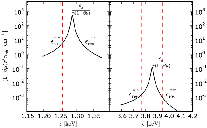
Figure 4.15: Dependence of the integrand from Equation 4.58 on the energy of the incident photon. Both panels were calculated for surface temperature $T=3\times 10^{6}\,{\rm K}$, cosine of the incident angle $\mu=0.1$ and Lorentz factor of particle $\gamma=10^{3}$. The left panel corresponds to resonance in magnetic field $B=10^{14}\,{\rm G}$, while the right panel was obtained using $B=3\times 10^{14}\,{\rm G}$.

Note that both plots do not include the dependence of the photon density on distance from the stellar surface. Depending on whether the radiation originates from the whole stellar surface or from the polar cap only, the dependence of the photon number density on the height above the surface can differ significantly (see Section 4.4.4).

4.4.3.2 Thermal-peak ICS

TICS includes all scattering processes of photons with frequencies around the maximum of the thermal spectrum. In our simulation we adopt $\epsilon_{{\rm{}_{th}}}^{{\rm{}^{min}}}\approx 0.05\epsilon_{{\rm{}_{th}}}$, and $\epsilon_{{\rm{}_{th}}}^{{}^{{\rm max}}}\approx 2\epsilon_{{\rm{}_{th}}}$ where $\epsilon_{{\rm{}_{th}}}=2.82kT/\left(mc^{2}\right)$ is the energy, in units of $mc^{2}$, at which blackbody radiation with temperature $T$ has the largest photon number density. The electron/positron mean free path for the TICS process can be calculated as

$$l_{{\rm TICS}}\approx\left[\int_{\mu_{0}}^{\mu_{1}}\int_{\epsilon_{{}_{{\rm th}}}^{{\rm{}^{min}}}}^{\epsilon_{{\rm{}_{th}}}^{{\rm{}^{max}}}}\left(1-\beta\mu\right)\sigma^{\prime}\left(\epsilon,\mu\right)n_{{\rm ph}}\left(\epsilon\right){\rm d}\epsilon{\rm d}\mu\right]^{-1}.$$ (4.60)

Figure 4.16 presents the dependence of the integrand from Equation 4.60 on photon energy for two different incident angles of background photons. As the number density depends exponentially on the photon energy, TICS is important only for small incident angles ($\mu\approx 1$). Note that for some specific combination of magnetic field strength, the Lorentz factor of the primary particle and the incident angle of background photons the resonance is in region of thermal peak. In such a case the resonant component is dominating (a much higher cross section) and the particle mean free path should be calculated using the approach described in the previous section.

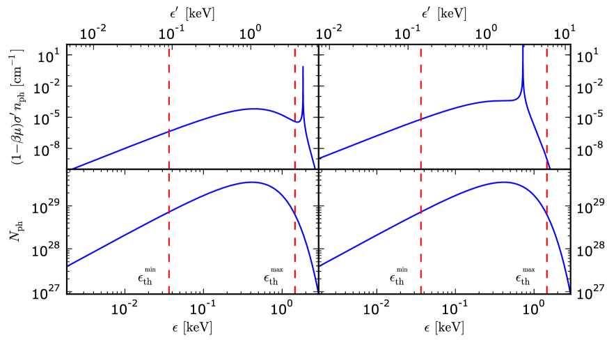
Figure 4.16: Comparison of the integrand from Equation 4.60 with photon number density. The bottom panels present the dependence of the photon number density on photon energy in OF. The red dashed lines correspond to limits used to calculate the particle mean free path for TICS. The top panels present the dependence of the integrand on photon energy in PRF. Both panels were obtained using surface temperature $T=3\times 10^{6}\,{\rm K}$, Lorentz factor of the particle $\gamma=10^{2}$ and magnetic field strength $B=10^{12}\,{\rm G}$. The cosine of the incident angle, $\mu=0.975$ and $\mu=0.96$, was used for the left and right panel, respectively.

4.4.3.3 Calculation results

For ultrastrong magnetic fields quite a wide range of the particle Lorentz factor falls into the peak of background photons (see Figure 4.17). In such a case RICS is enhanced by the fact that it involves photons with very high density. Furthermore, the RICS process for such particles is indistinguishable from the TICS (see Figure 4.16). For particles with Lorentz Factor $\gamma\gtrsim 10^{5}$, the dominant process of radiation is CR. The exact value of this limit depends on conditions such as: density of background photons, incident angles between particles and photons, and curvature of magnetic field lines ($1/\Re$).

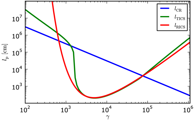
Figure 4.17: Dependence of a particle mean free path on its Lorentz factor for three different processes: CR, RICS and TICS. The calculations were performed for magnetic field strength $B_{14}=2$, radius of curvature of magnetic field lines $\Re_{6}=1$ (for the CR process) and hot spot temperature $T_{6}=3$ (for RICS and TICS). Both RICS and TICS were calculated for a full range of incident angles ($\mu_{0}=0$, $\mu_{1}=1$). Note that for a Lorentz factor in the range of $\gamma\approx 2\times 10^{3}-10^{5}$ the particle mean free paths of RICS and TICS are equal as the resonance falls into the peak of the background photons.

Figure 4.18 presents the dependence of a particle mean free path on the magnetic field strength and the particle Lorentz factor for RICS. The minimum of the mean free path for relatively weak magnetic fields ($B_{14}=0.5$) is for particles with Lorentz factor $\gamma\approx 2\times 10^{3}$, while for relatively stronger magnetic fields ($B_{14}=3.5$) the RICS is most efficient for particles with energy an order of magnitude larger ($\gamma\approx 2\times 10^{4}$). This is a natural consequence of the fact that resonance takes place when the photon energy in PRF is equal to the electron cyclotron energy, which in stronger fields is higher. As can be seen from the Figure, the particle mean free paths for RICS in stronger magnetic fields increase. This is due to the decreasing resonant cross section with increasing magnetic field strength (see Figure 4.15). Note, however, that this behaviour does not include the fact that photon density in regions with weaker magnetic fields is considerably smaller. In fact, the results of the cascade simulation presented in Chapter 5 show that RICS is efficient only in the immediate vicinity of a neutron star since photon density at higher altitudes drops rapidly.

Figure 4.18: Dependence of a particle mean free path on magnetic field strength ($B_{14}$) and the Lorentz factor of a particle ($\gamma$) for the RICS process. The particle mean free path was calculated for semi-isotropic blackbody radiation ($\mu_{0}=0$, $\mu_{1}=1$) with temperature $T_{6}=2.5$.

4.4.4 Background photons

4.4.4.1 Photon density

One of the main parameters affecting ICS above the stellar surface is photon density. The initial photon density (at altitude $z=0$) highly depends on the temperature of the radiating surface. As shown in Chapter 1 (e.g. see Table 1.4), the entire surface has the lowest temperature ($T_{6}\lesssim 0.8$), thus the initial photon density is up to about two orders of magnitude lower than warm spot radiation ($T_{6}\lesssim 3$) and up to about three orders magnitude lower than hot spot radiation ($T_{6}\lesssim 5$). However, the density of the photons strongly depends on the distance from the source of radiation (especially for the hot spot). Therefore, we used the simplified method presented in Figure 4.19 to calculate photon density at a given point $L=\left(r,\,\theta,\,\phi\right)$. Then the relative density of photons originating from the entire surface can be calculated as

$$\frac{n_{{\rm st}}\left(\epsilon,\,T_{{\rm st}},\,L\right)}{n_{0}\left(\epsilon,\,T_{{\rm st}}\right)}=\sin^{2}\left(\frac{\Delta\theta_{{\rm st}}}{2}\right)=\left(\frac{R}{r}\right)^{2},$$ (4.61)

where $n_{{\rm st},0}\left(\epsilon,\,T_{{\rm st}}\right)$ is the density of photons with energy $\epsilon$ at the stellar surface with temperature $T_{{\rm st}}$, and $\Delta\theta_{{\rm st}}$ is the angular diameter of the star at a distance from the star centre $r$.

Likewise, we can write a formula for the relative density of photons originating from a spot (warm or hot) as

$$\frac{n_{{\rm sp}}\left(\epsilon,\,T_{{\rm sp}},\,L\right)}{n_{{\rm sp},0}\left(\epsilon,\,T_{{\rm sp}}\right)}=\sin^{2}\left(\frac{\Delta\theta}{2}\right),$$ (4.62)

where $n_{{\rm sp},0}\left(\epsilon,\,T_{{\rm sp}}\right)$ is the density of photons with energy $\epsilon$ at the spot surface (either hot or warm) with temperature $T_{{\rm sp}}$. The angular diameter of the spot can be calculated as

$$\Delta\theta=\arccos\left(\frac{r_{1}^{2}+r_{2}^{2}-4R_{{\rm sp}}}{2r_{1}r_{2}}\right),$$ (4.63)

here $R_{{\rm sp}}$ is the spot radius and $r_{1}$, $r_{2}$ are the distances to the outer edges of the spot (see Figure 4.19).

Figure 4.19: Simplified method used for calculation of a photon density originating from an entire stellar surface (blue lines) and from a hot/warm spot (red lines). Here $R_{{\rm sp}}$ is a spot radius (either hot or warm). Let us note that the simplified method is valid for the entire surface component regardless of the $\phi$ component of location $L$, while for the spot component it can be used only for small values of $\phi$. In a more general case the spot should be projected on the surface perpendicular to the radius vector ${\bf r}$ and passing through point $L$.

Figure 4.20 presents the dependence of the relative photon density ($n\left(z\right)/n_{0}$) on the distance from the stellar surface. Due to the small size of a polar cap (hot spot, $R_{{\rm hs}}=50\,{\rm m}$) the density of the photons drops rapidly and already at a distance of about $z=150\,{\rm m}$ it is one order of magnitude lower than at the polar cap surface. On the other hand, for a larger size of the warm spot ($R_{{\rm hs}}=1\,{\rm km}$) the photon density is reduced by an order of magnitude at a distance of about $z=3\,{\rm{\rm km}}$. From Equation 4.61 it can easily be seen that the photon density of radiation from the entire stellar surface decreases by an order of magnitude at a distance of about $z\approx 3R\approx 30\,{\rm km}$.

Figure 4.20: Dependence of the relative photon density on the distance from the stellar surface for three different thermal components (the entire stellar surface, the warm spot and the hot spot). The following parameters were used for the calculations: star radius $R=10\,{\rm km}$, warm spot radius $R_{{\rm ws}}=1\,{\rm km}$ and hot spot radius $R_{{\rm hs}}=50\,{\rm m}$.

The very small size of the polar cap also has an additional implication to the background photons’ density. Namely, the density of the background photons just above the polar cap highly depends not only on the distance from the surface, but also on the position relative to the cap centre.

Figure 4.21 presents the dependence of the relative photon density originating from a polar cap (the hot spot) on the distance from the stellar surface for three different starting points on the polar cap. The distance was calculated for points which follow the magnetic field structure of PSR B0656+14. Note that for the extreme magnetic line (which starts at the cap edge) already at a distance of about $z_{2}\approx 5\,{\rm m}$ the photon density decreases twice, while for the central ($\theta_{0}$) and middle line ($\theta_{1}$) the distances are respectively $z_{0}\approx 45\,{\rm m}$ and $z_{1}\approx 30\,{\rm m}$. This result is important as the background photon density directly translates to the particle mean free path in ICS (see Section 4.4.3). This means that for ICS-dominated gaps the sparks’ height will vary depending on their location. The breakdown of the gap (spark) in the central region of a polar cap is easier to develop as the particle mean free path is lower, and eventually it will result in lower heights of the central sparks. This will influence the properties of plasma produced in the central region of open magnetic field lines, and depending on the conditions may result in the formation of plasma either suitable to produce radio emission (core emission) or unsuitable to produce radio emission (conal emission but with the line of sight crossing the centre of the beam).

To find the dominant component of thermal radiation at a given altitude we need to take into account the initial flux of radiation and how it changes with the distance. Below we present the calculations of a radiation flux (Figure 4.22) for PSR B0656+14. The parameters of an entire surface and warm spot components are in agreement with the observations (see Table 1.4), while the hot spot component was calculated using parameters derived from the modelling of a non-dipolar structure of the magnetic field (see Chapter 2).

Figure 4.21: Dependence of the relative photon density on the distance from the stellar surface for a hot spot component of PSR B0656+14. The relative photon density was calculated for three different starting positions: $\theta_{0}$ (central), $\theta_{1}$ (at the half distance to the edge), and $\theta_{2}$ (the cap edge). The altitude ($z$) was calculated for points which follow the magnetic field structure of PSR B0656+14.

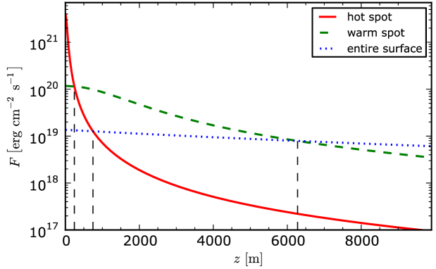
Figure 4.22: Dependence of the radiation flux for three different components (the entire stellar surface, the warm spot and the hot spot) on the distance from the stellar surface for PSR B0656+14. The following parameters were used for the calculations: entire stellar surface radiation, $T_{{\rm st}}=0.7\,{\rm MK}$, $R_{{\rm st}}=20\,{\rm km}$; warm spot, $T_{{\rm ws}}=1.2\,{\rm MK}$, $R_{{\rm ws}}=1.8\,{\rm km}$; and hot spot, $T_{{\rm hs}}=2.9\,{\rm MK}$, $R_{{\rm hs}}=50\,{\rm m}$.

Already at a distance of $240\,{\rm m}$ the flux of the warm spot radiation becomes higher than the flux of the hot spot radiation. Furthermore, already at a height of $750\,{\rm m}$ flux the radiation originating from the polar cap (hot spot) becomes lower than the flux of radiation from the entire stellar surface. With an increasing distance the flux of the warm spot decreases faster than the flux of the entire surface radiation and at a distance of $6.3\,{\rm km}$ the thermal radiation from the entire stellar surface becomes the dominant component of the background photons.

The results may suggest that up to a height of about $240\,{\rm m}$ (for PSR B0656+14) the hot spot radiation should be the main source of the background photons involved in ICS. However, the actual height is smaller as the results do not include the efficiency of ICS, which also depends on the incident angle between the photons and the particles (see the next Section).

4.4.4.2 Photon incident angles

Another parameter that significantly affects the ICS is the incident angle between the background photons and the relativistic particles. Especially for Resonant Inverse Compton Scattering is the incident angle of great importance. Figure 4.23 presents the dependence of a particle mean free path for ICS on a maximum value of the incident angle $\psi_{{\rm crit}}$. If incident angles are low, the resonance is outside of the photon spectrum and results in very high values of particle mean free paths. The lower the energy of the particle (lower Lorentz factor), the incident angles should be larger to ensure that the resonance falls into an energy range with high photon density.

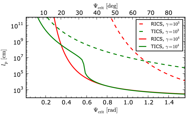
Figure 4.23: Dependence of the particle mean free path on the maximum value of the incident angle $\psi_{{\rm crit}}$. The particle mean free path $l_{{\rm p}}$ was calculated for magnetic field strength $B=10^{14}\,{\rm G}$ assuming background blackbody radiation with a temperature $T=3\,{\rm MK}$. Two different particle Lorentz factors were used for the calculations: $\gamma=10^{3}$ (dashed lines) and $\gamma=10^{4}$ (solid lines). The red lines correspond to Resonant Inverse Compton Scattering, while the blue lines correspond to Thermal-peak Inverse Compton Scattering.

TICS for a given magnetic field strength and the Lorentz factor of particles is not significant (high particle mean free paths) unless the angles of the incident photons are high enough. Note the characteristic drop of the particle mean free path for TICS at $\psi_{{\rm crit}}\approx 20^{\circ}$ (for $\gamma=10^{4}$) and $\psi_{{\rm crit}}\approx 75^{\circ}$ (for $\gamma=10^{3}$). For such high incident angles the resonance takes place at the thermal peak of the background photons. Therefore, TICS and RICS are indistinguishable, which results in an almost equal particle mean free path (see the text above Figure 4.16 for more details).

Due to the very small size of the polar cap the influence of the hot spot component will by lower not only because of the change of photon density, but also because of the rapid change of the incident angle between the photons and particles. Figure 4.24 presents the dependence of the maximum incident angle on the altitude above the stellar surface for three thermal components (the entire surface, the warm spot and the hot spot). As follows from the Figure, already at an altitude of $z\approx 90\,{\rm m}$ does the maximum value of the incident angle between the photons from the hot spot and the particles drop to $\psi_{{\rm crit}}=30^{\circ}$, which significantly lowers the efficiency of ICS for this source of background photons (see Figure 4.23). Since the size of the warm spot component is larger, the warm spot radiation will be significant for up to higher altitudes, but already at a distance of $z\approx 1.5\,{\rm{\rm km}}$ the maximum value of the incident angle also drops to $\psi_{{\rm crit}}=30^{\circ}$.

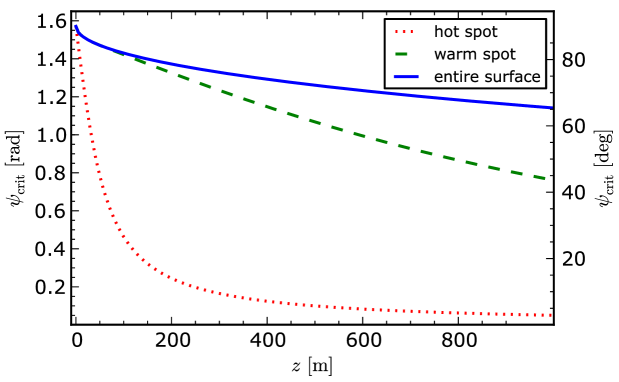
Figure 4.24: Dependence of the maximum incident angle on the altitude above the stellar surface for three thermal components (the entire surface, the warm spot and the hot spot radiation).

Note that in the Figure we have calculated the maximum value of the intersection angle at altitudes which correspond to radial progression from the stellar surface. In fact, the actual maximum value of the incident angle also depends on the structure of the magnetic field. Figure 4.25 presents the actual maximum value of the incident angle of photons originating from the hot spot for three different magnetic field lines calculated for PSR B0656+14. The actual values of the maximum incident angle just above the surface exceed $90^{\circ}$, but its rapid decline (especially for extreme lines) causes the radiation of the hot spot component to become insignificant for ICS at relatively low altitudes $z\approx 20\,{\rm m}$.

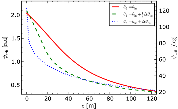
Figure 4.25: Dependence of the maximum incident angle on the altitude above the stellar surface for the hot spot component of PSR B0656+14. The maximum incident angle was calculated for three different starting positions: $\theta_{0}$ (central), $\theta_{1}$ (at the half distance to the edge), and $\theta_{2}$ (the cap edge).

Both the decrease of photon density and the decrease of the maximum inclination angle cause the parameters of plasma produced by RICS to highly depend on the properties (size and temperature) of the background photons source. The hot spot component will be the dominant source of background photons for ICS in the gap region ($z\lesssim 20\,{\rm m}$), while the radiation of the warm spot and the entire surface will be the main source of the background photons for ICS at higher altitudes.

Chapter 5 Physics of pulsar radiation

5.1 Inner Acceleration Region

5.1.1 Gamma-ray emission

In our model most of the $\gamma$-photons are produced in the Inner Acceleration Region or in close vicinity of a neutron star. Due to an ultrastrong surface magnetic field, the most energetic $\gamma$-photons are produced by Inverse Compton Scattering in the PSG-on mode. If a pulsar is in the PSG-off mode, Curvature Radiation produces fewer energetic photons than ICS in the PSG-on mode. Photons produced in IAR (both the ICS and CR) are absorbed by strong magnetic fields creating positron-electron plasma in the gap region, thereby enhancing a cascade, or just above the gap enhancing a secondary plasma population. The absorption of $\gamma$-photons in close vicinity of NS makes it impossible to directly observe the radiation produced in IAR. However, a characteristic of this emission defines the parameters of the gap (e.g. multiplicity in the gap region, gap height, etc.), and thus the parameters of secondary plasma.

5.1.1.1 PSG-off mode

In general, the existence of high potential in IAR (e.g. wide sparks or $\eta\approx 1$) results in solutions for which CR is responsible for the emission of $\gamma$-photons. The energy of such radiation depends on the Lorentz factor of primary particles and curvature of the magnetic field lines. Figures 5.1 and 5.2 present the histogram of photons produced in IAR by CR for PSR B0628-28 and Geminga, respectively. The curvature in IAR of Geminga is lower ($\Re_{6}\approx 2.1$, see Section 2.4.2), thus the primary particle should be accelerated to higher energies in order to produce the required number of photons in the gap region. Eventually the higher Lorentz factor of primary particles will result in the emission of $\gamma$-photons with energy up to $10\,{\rm GeV}$ for Geminga. On the other hand, the curvature magnetic lines for PSR B0628-28 ($\Re_{6}=0.6$, see Section 2.4.1) is higher, which reduces the photon mean free path and it is possible to produce the required number of photons in the gap region $N_{{\rm ph}}^{{\rm CR}}$ for lower the Lorentz factor of primary particles.

In CR-dominated gaps we can distinguish three types of photons: (I) radiation with energy below $1\,{\rm MeV}$ which is unaffected by the magnetic field (except the splitting) and can be detected by a distant observer, (II) soft $\gamma$-ray photons which create pairs above ZPF, (III) and high energetic $\gamma$-photons responsible for pair production below ZPF. In an ultrastrong magnetic field the photons from the third group will produce particles just after reaching the first threshold. Due to the fact that most CR photons are $\parallel$-polarised, photon splitting is insignificant in cascade pair production in the PSG-off mode.

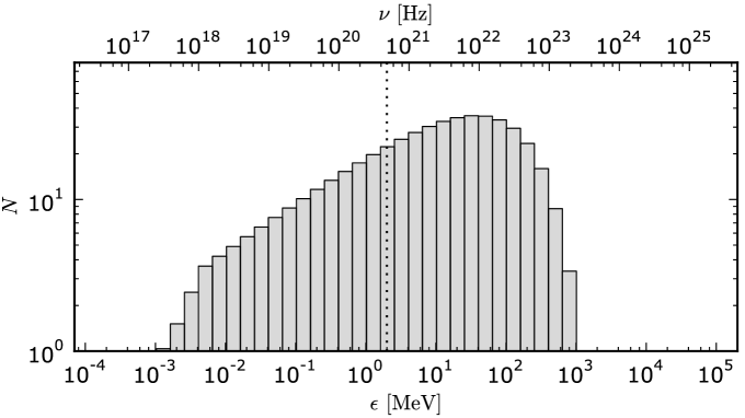
Figure 5.1: Distribution of photons produced in IAR by a single particle for PSR B0628-28. In the calculations we used parameters of the gap in the PSG-off mode as presented in Table 3.1. We also assumed a linear change in the acceleration electric field (see Equation 3.27).

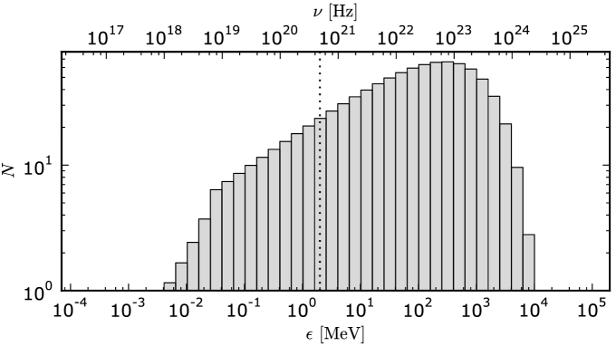
Figure 5.2: Distribution of photons produced in IAR by a single particle for PSR J0633-1746. In the calculations we used parameters of the gap in the PSG-off mode as presented in Table 3.1.

5.1.1.2 PSG-on mode

When the acceleration potential is low enough (narrow sparks with $\eta<1$) to satisfy the condition for effective ICS ($l_{{\rm ICS}}\lesssim l_{{\rm acc}}$), the gap will operate in the PSG-on mode. The energy of ICS radiation in the gap region (RICS) depends on the Lorentz factor of primary particles and the strength of magnetic field. In an ultrastrong magnetic field of IAR implied by the PSG model, the primary particle loses most of its energy during the scattering of background photons. Such extremely energetic photons produce pairs on the zero-th Landau level ($\parallel$-polarised photons) or split to less energetic photons before reaching the first threshold (see Section 4.2.6). After the photons split the resulting photons are still very energetic and create an electron-positron pair enhancing the avalanche production of particles. In contrast to the PSG-off, most of the electron-positron pairs in the PSG-on mode are created well below ZPF. Furthermore, there is no additional radiation at lower energies ($\epsilon<1\,{\rm MeV}$) which could be detected by a distant observer. Figures 5.3 and 5.4 present the distribution of photons produced by the first population of newly created particles for PSR B0950+08 and PSR B1929+10, respectively. In both cases the energy of the $\gamma$-photons ranges from $1\,{\rm GeV}$ to $\approx 20\,{\rm GeV}$. The narrow predicted spark half-width of PSR B0950+08 results in a lower potential in IAR, thus increasing the efficiency of ICS (more photons produced by the first population of particles). The particle mean free path for ICS is smaller for backstreaming particles (see Section 3.2.1 for more details), thus most photons in the PSG-on mode are produced in the direction towards the stellar surface. Note that not all photons will produce electron-positron pairs since some $\gamma$-photons are produced so close to the stellar surface that they reach its surface before they manage to reach the first threshold for pair production.

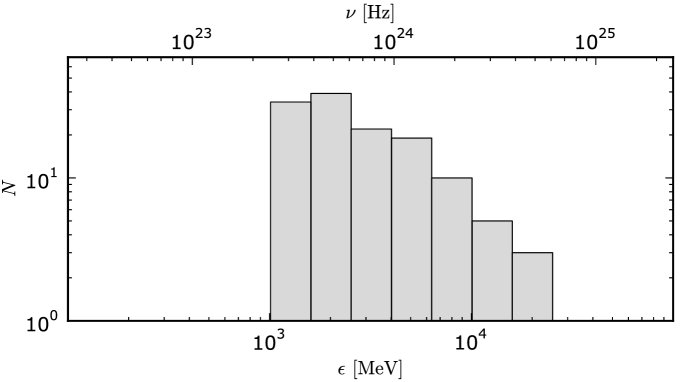
Figure 5.3: Distribution of photons produced in IAR by the first population of newly created particles for PSR B0950+08. In the calculations we used the parameters of the gap in the PSG-on mode as presented in Table 3.1.

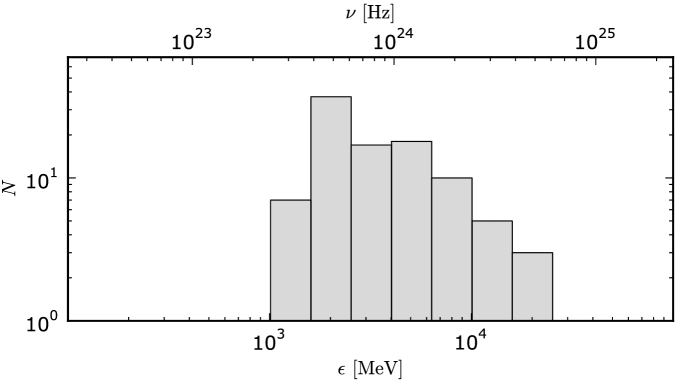
Figure 5.4: Distribution of photons produced in IAR by the first population of newly created particles for PSR B1929+10. In the calculations we used the parameters of the gap in the PSG-on mode as presented in Table 3.1.

5.1.2 X-ray and less energetic emission

An negligible fraction of energy radiated by a primary particle in the PSG-off mode falls in the X-ray band. What is more, in the PSG-on mode all photons produced by ICS have energy which exceeds an electron’s rest energy by many orders of magnitude. Thus, IAR may be responsible only for generating the thermal component of the X-ray spectrum in the process of heating the stellar surface.

5.1.2.1 Thermal emission

As shown in Section 1.4, thermal emission is a common feature of neutron stars. Due to the large uncertainties in X-ray observations, it is not possible to distinguish all three thermal components (entire surface radiation, warm spot component and hot spot radiation) for one specific pulsar. Furthermore, only for a few pulsars (e.g. Geminga, PSR B0656+14) was it possible to distinguish two thermal components alongside the nonthermal one. In this thesis we focus on an analysis of pulsars with a visible hot spot component ($b>1$), since only for these pulsars is it possible to estimate the size of the actual polar cap. Most of these pulsars are old neutron stars and only for one of them (Geminga) was the whole surface radiation found in the X-ray spectrum. Figure 5.5 presents the observed X-ray components of the Geminga pulsar: the whole surface radiation, the polar cap (hot spot) and the nonthermal component. The maximum of energy for the whole surface radiation is in extreme ultraviolet and in soft X-rays for the hot spot component. Taking into account the very small area of the polar cap, radiation from the hot spot is unlikely to be observed in wavelengths off the maximum.

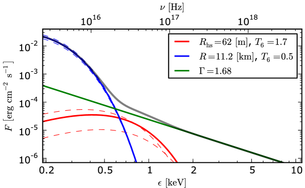
Figure 5.5: Observed flux of radiation for PSR J0633+1746. In the figure we present three components of radiation: the nonthermal one (green line), the entire surface radiation (blue line), and the hot spot component (red line). The dashed lines correspond to uncertainties in observations (see Table 1.4).

Figure 5.6 presents the X-ray spectrum of PSR B1133+16. The small number of counts detected resulted in the fact that only separate fits for the BB and PL components were performed. Both the BB and PL fits describe the observed spectrum with similar accuracy. In the Figure we present additional thermal components (the entire surface radiation and the warm spot) which have not been determined by the observations. The Figure shows that the overlapping thermal components can mimic the power-law dependence of the spectrum at frequencies below $2\,{\rm keV}$.

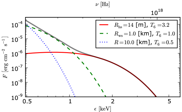
Figure 5.6: X-ray spectrum of PSR B1133+16. In addition to the observed thermal radiation (red solid line), two other thermal components are presented: the warm spot radiation (green dashed line) and the entire surface radiation (blue dotted line).

Although this specific combination of thermal components for PSR B1133+16 would result in a photon index greater than the observed one $\Gamma=2.51$, the spectral fits for all pulsars should be extended to include more BB components in order to examine the effect of thermal components overlapping at lower frequencies. The results of our calculations suggest that the nonthermal X-ray radiation should dominate the spectrum at higher frequencies $\approx 3-10\,{\rm keV}$, but the power-law-like behaviour at lower frequencies could be the result of the overlapping of thermal components anticipated in the PSG scenario (see Section 5.1.2.3).

5.1.2.2 Nonthermal emission

The polarisation of ICS radiation in an ultrastrong magnetic field is $50\%$ (one $\parallel$ to every $\perp$-polarised photon). Synchrotron Radiation of secondary particles created by $\perp$-polarised photons would generate hard X-ray photons, however, as was mentioned in Section 4.2.6, these photons will split before they reach the first threshold to produce pairs. Therefore, regardless of whether the gap is dominated by CR or by ICS, Synchrotron Radiation in IAR is not significant.

5.1.2.3 Warm spot component

Apart from the obvious X-ray component corresponding to the whole surface radiation, the PSG model can explain both the hot and warm spot radiation. The hot spot radiation is a natural consequence of heating the actual polar cap region by the backstreaming particles (see Section 1.4.4). As was mentioned in Section 1.4.4, the warm spot component can have two different sources: (I) the drastic difference of the crustal transport process due to the non-dipolar structure of the surface magnetic field (for young and middle-aged pulsars), (II) and a mechanism of heating the surface adjacent to the polar cap. In this section we present the second mechanism, i.e. heating of the surface adjacent to the polar cap, which can be applied to both young and old pulsars.

Figure 5.7 presents the mechanism of heating the area adjacent to the polar cap for PSR B0950+08. When the gap operates in the PSG-off mode the primary plasma (see Section 5.1.3) will lose a significant part of its energy via CR as the particles propagate through the region of high curvature. For this particular magnetic line’s configuration the region of high CR extends up to an altitude about $4\,{\rm km}$ above the stellar surface. The most energetic CR photons emitted in this region have a relatively short mean free path and they produce electron-positron pairs in the region of open magnetic field lines. However, both the less energetic CR photons and $\gamma$-photons produced by SR have a large enough photon mean free path to produce pairs in the region of the closed magnetic field lines. All newly created pairs move along the closed magnetic field lines and heat the surface beyond the polar cap on the opposite side of the star.

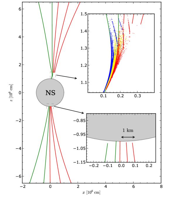
Figure 5.7: Global structure of magnetic field lines for PSR B0950+08. The structure was obtained using two crust-anchored anomalies (see Section 2.4.5). Green lines correspond to the outer open magnetic field lines, while the red lines correspond to the closed magnetic field lines at which secondary pairs are produced. Blue, yellow and red dots represent the locations of secondary pair production for the outer left, the middle and the outer right open field lines, respectively.

The fraction of energy transferred to the region of the closed field lines highly depends on the region of open magnetic field lines considered in CR/SR emission. In the Figure we use three different colours (blue, yellow and red) to show the positions of pair creation for three characteristic open magnetic field lines (the outer left, the middle and the outer right). The simulation results in the following fractions of energy transferred to the region of the closed field lines are: $0.02\%$, $0.1\%$, $6\%$ for all three lines, respectively. For this specific magnetic field configuration the transferred energy fraction increases as we move towards the region with the highest curvature. We can roughly estimate that for the proposed magnetic field configuration of PSR B0950+08, about $1\%$ of the outflowing energy is responsible for heating of the surface beyond the polar cap on the opposite side of the star. Note that due to strong anisotropy of the outflowing and backflowing stream of particles (see Section 5.1.3), this fraction could be enough to obtain the warm spot component with a luminosity equal or in some cases even higher than the luminosity of the hot spot component.

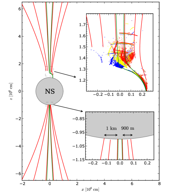
Figure 5.8: Global structure of magnetic field lines for PSR B0943+10. The structure was obtained using two crust-anchored anomalies (see Section 2.4.4). Green lines correspond to the outer open magnetic field lines, while the red lines correspond to the closed magnetic field lines at which secondary pairs are produced. Blue, yellow and red dots represent the locations of secondary pair creation for the outer left, the middle and the outer right open field lines, respectively.

The fraction of energy transferred to the region of closed field lines highly depends on the magnetic field configuration. A more complicated structure of the magnetic field lines proposed for PSR B0943+10 (see Figure 5.8) results in a much wider area of closed field lines at which pairs are created, and hence higher fractions of energy transferred to the region of closed field lines. For this specific structure of the magnetic field these fractions are: $7\%$, $1\%$, $2\%$ for three characteristic lines, respectively. We can roughly estimate that about $3-5\%$ of the outflowing energy is responsible for the heating. Note that the magnetic field structure of PSR B0950+08 results in the heating of only one side beyond the polar cap, while in the case of PSR B0943+10 the whole surface around the polar cap is heated. The actual size of the warm spot also depends on the magnetic field configuration in the heating zone, and can either be decreased or increased.

5.1.3 Primary plasma

As we mentioned in Section 3.2.2, PSG-off and PSG-on modes differ essentially by the Lorentz factor of primary particles produced in the gap region. Furthermore, different scenarios of the gap breakdown (due to surface overheating or due to production of dense enough plasma) cause the evolution of primary particles in the two modes to completely different.

We assume that in the PSG-off mode the gap breakdown is due to surface overheating; hence the plasma cloud moving away from the stellar surface is a mixture of ions and electron-positron plasma. In this scenario the ions are the main source of charge density required to screen the gap (see Equation 3.40). As the plasma cloud moves away from the stellar surface both the spark height and the spark width increase, which results in an increase of the acceleration potential drop. When the particles gain the Lorentz factors $\gamma\gtrsim 10^{5}$, CR begins to produce $\gamma$-photons. In the PSG-off mode most of the $\gamma$-photons are created near ZPF (see Figure 3.4). All particles created by $\gamma$-photons above the ZPF do not contribute to the heating of the surface. Furthermore, the acceleration in the upper parts of the gap is relatively weak, and electrons produced in this region will also escape from the gap, thus not contributing to the surface heating. Depending on the details of the cascade formation, the process described above may result in the creation of strong streaming anisotropies, where the flux of the backstreaming particles is considerably smaller than the flux of the outstreaming particles. Note that the density of the backstreaming particles required to overheat the surface is significantly lower than the co-rotational density $n_{{\rm CR}}\ll n_{{\rm GJ}}$ (see Table 3.1).

In the PSG-on mode the quasi-equilibrium of the flux of backstreaming particles and the flux of the polar cap radiation can cause the gap to break only due to the production of dense enough plasma. Thus, the surplus of positrons is the main source of the charge in the plasma cloud moving away from the stellar surface. The ICS process responsible for the cascade production of particles is effective only in the bottom part of the gap. Hence, the backstreaming electrons will hit the surface with a Lorentz factor $\gamma_{{\rm c}}$ well below the $\gamma_{{\rm max}}$. As there is no strong pair production near (or above) ZPF, the backstreaming/outstreaming anisotropy arises only due to the difference of the Lorentz factor of electrons hitting the stellar surface and the Lorentz factor of positrons accelerated in the gap $\gamma_{{\rm max}}/\gamma_{{\rm c}}\approx 10$. The actual density of newly created plasma to completely screen the gap can be calculated only in the full cascade simulation. However, as shown by Timokhin, (2010), this density should significantly exceed the co-rotational Goldreich-Julian density $n_{{\rm ICS}}\gg n_{{\rm GJ}}$. We describe the difference between the co-rotational density and the actual density of primary plasma required to completely screen the ICS-dominated gap by factor $N_{{\rm ICS}}=n_{{\rm ICS}}/n_{{\rm GJ}}\gg 1$.

5.2 Inner magnetosphere of a pulsar

5.2.1 Gamma-ray emission

In general there are three processes which can produce $\gamma$-ray emission in the inner magnetosphere of a pulsar ($R_{{\rm pc}}\ll z\ll R_{{\rm LC}}$): CR, ICS and SR. Which of them produces the majority of $\gamma$-photons depends on the parameters of the primary particles, and thus mainly depends on the mode in which the gap operates. Additionally, the efficiency of the ICS process strongly depends on the source of the background photons.

5.2.1.1 Curvature Radiation of primary particles

When the gap operates in the PSG-off mode, high-energetic particles are produced $\gamma_{{\rm c}}\gtrsim 10^{6}$. As they pass the region with high curvature ($\Re_{6}\approx 1$) they radiate a significant part of their energy through CR (see Section 4.1).

Figure 5.9 presents the distribution of CR photons produced by a single primary particle moving along the open magnetic field line of PSR B1133+16 (see Section 2.4.5 for the details of the magnetic field configuration). The initial Lorentz factor of the particle $\gamma_{{\rm max}}=1.7\times 10^{6}$ was set according to the value presented in Table 3.1. As the particle advanced through the region with high curvature, it lost about $46\%$ of its initial energy, which was mainly converted to high-energetic $\gamma$-photons with an energy up to about $2\,{\rm GeV}$. The $\gamma$-photons are produced in a region of a strong magnetic field, thus after passing a relatively short distance the most energetic photons are absorbed by the magnetic field and electron-positron pairs emerge. The red colour in the Figure corresponds to the final spectrum (after photon splitting, pair production and SR) produced by a single primary particle in the PSG-off mode. Most of the energy radiated by the primary particle was converted into the secondary plasma (see Section 5.2.3) and only about $5\%$ of the particle’s initial energy ended in the form of radiation with a cut-off at about $30\,{\rm MeV}$.

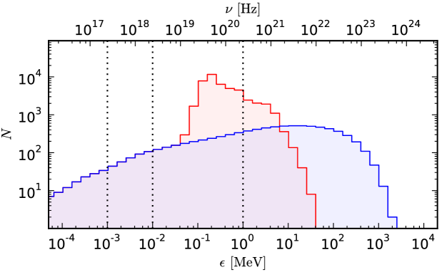
Figure 5.9: Final photon distribution produced by a single primary particle for PSR B1133+16. The blue line corresponds to the initial CR distribution, while the red line presents the final distribution with the inclusion of photon splitting, pair production and SR.

To increase the amount of photons reaching the observer, the emission zone, i.e. the region with the highest curvature, should by located in the area with a weaker magnetic field. Such a configuration allows a photon to travel a longer distance before it is absorbed by the magnetic field. As a result the electron-positron pairs are created at higher Landau levels, which enhances SR. Figure 5.10 presents the distribution of CR photons for PSR B0950+08. The calculations were performed for the initial Lorentz factor of the particle $\gamma_{{\rm max}}=2.0\times 10^{6}$ (see Table 3.1).

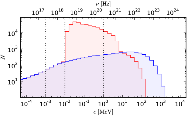
Figure 5.10: Final photon distribution produced by a single primary particle for PSR B0950+08. The blue line corresponds to the initial CR distribution, while the red line presents the final distribution with the inclusion of photon splitting, pair production and SR.

Due to CR the primary particle lost about $40\%$ of its initial energy. In this case about a half of the energy radiated by the primary particle was converted into the secondary plasma and the same amount of energy (about $20\%$ of the particle’s initial energy) ended in the form of radiation. For both PSR B1133+16 and PSR B0950+08, the maximum of the curvature is of the same order. However, the maximum of curvature for PSR B1133+16 is located at an altitude of about $800\,{\rm m}$, while for PSR B0950+08 it is located at an altitude of about $1.75\,{\rm km}$ (compare Figures 2.23 and 2.20).

5.2.1.2 Inverse Compton Scattering of primary particles

In the PSG-on mode the maximum Lorentz factor of primary particles is in the range of $10^{4}-10^{5}$ (see Table 3.1). As it follows from Figures 4.17 and 4.18, the ICS process is most effective for particles with a Lorentz factor in the range of $10^{3}-10^{4}$. Particles with high energies ($\gamma\gtrsim 10^{5}$) will upscatter thermal photons only just above the stellar surface, where the density of the background photons is very high (see Section 5.1.1.2). Thus, if there is no additional source of background photons, the most energetic particles ($\gamma\gtrsim 10^{5}$) will escape from the inner magnetosphere without losing their energy by ICS. However, the plasma cloud produced by the ICS-dominated gap has a density exceeding the co-rotational Goldreich-Julian density even by a few orders of magnitude (see Section 5.1.3). Such a high charge density reduces the acceleration (Timokhin,, 2010) and, consequently, the bulk of particles will escape from the IAR with lower Lorentz factors. It is not possible to estimate the actual Lorentz factor of particles in the plasma cloud at the moment of gap breakdown without performing a full cascade simulation. Thus, in this thesis we assume that at the moment of gap breakdown most of the particles will have an energy that is about the characteristic value at which the acceleration is stopped by ICS in the bottom parts of the IAR $\gamma_{{\rm c}}$. To increase readability for cascade simulations with very low surface temperature, in all the Figures of the ICS distribution we present $\gamma$-photons produced by $50$ primary particles with Lorentz factors in the range of $0.5\gamma_{{\rm c}}-2\gamma_{{\rm c}}$.

In Figure 5.11 we present the distribution of ICS photons produced by the upscattering of surface thermal radiation with temperature $T_{{\rm s}}=0.3\,{\rm MK}$ for PSR B0834+06. Even for such a low surface temperature the whole surface radiation is the dominant source of background photons for ICS up to altitudes of about one stellar radii. During the scattering the primary particles lose about $30\%$ of their initial energy while producing $\gamma$-photons with energy up to $1\,{\rm GeV}$. Since the $\gamma$-photons are very energetic and are produced in a region with a strong magnetic field, they will be absorbed by the magnetic field, thus giving rise to the secondary plasma population (see Section 5.2.3). All pairs in the inner magnetosphere of a pulsar are created in the nonzero Landau level, thus the pair production process is also accompanied by strong SR (see the next section).

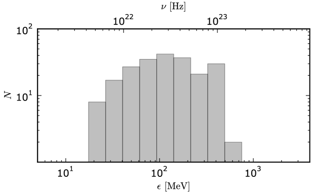
Figure 5.11: Distribution of ICS photons produced by an upscattering of surface radiation ($T_{{\rm s}}=0.3\,{\rm MK}$) for PSR B0834+06. The plot includes all $\gamma$-photons upscatterd by $50$ primary particles with Lorentz factors in the range of $2.5\times 10^{3}-10^{4}$.

A natural way of increasing the number of $\gamma$-photons produced by ICS in the inner magnetosphere is to increase the number of background photons. Figure 5.12 presents the distribution of ICS photons produced by an upscattering of the surface thermal radiation with temperature $T_{{\rm s}}=0.4\,{\rm MK}$ for PSR B0834+06. During the ICS process the primary particles lose about $65\%$ of their initial energy. For higher surface temperatures the ICS produces $\gamma$-photons up to higher altitudes (about two stellar radii), thus photons with lower energy emerge $\epsilon_{{\rm min}}\approx 3\,{\rm MeV}$. These less energetic photons will reach the observer, but their total energy is significantly lower than the total energy of the secondary plasma created by more energetic $\gamma$-photons.

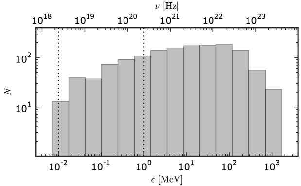
Figure 5.12: Distribution of ICS photons produced by an upscattering of the surface radiation ($T_{{\rm s}}=0.4\,{\rm MK}$) for PSR B0834+06. The plot includes all $\gamma$-photons upscatterd by $50$ primary particles with Lorentz factors in the range of $2.5\times 10^{3}-10^{4}$.

Note that although for PSR B0834+06 the X-ray spectral fit was performed with only one BB component, the surface temperatures used in the calculations ($0.3\,{\rm MK}$ and $0.4\,{\rm MK}$) are in good agreement with the predicted surface temperature of an old neutron star.

Another source of background photons which could be relevant for ICS in the inner magnetosphere is the warm spot component. As shown in Section 5.1.2.3, if the antipodal spot operates in the PSG-off mode and if the magnetic field structure is suitable then the warm spot is formed in the region adjacent to the polar cap. With a temperature lower than the hot spot but a much larger area, the warm spot is the main source of the background photons at altitudes up to about half a stellar radius.

In Figure 5.13 we present the distribution of ICS photons produced by an upscattering of warm spot radiation with temperature $T_{{\rm s}}=1.0\,{\rm MK}$ and radius $R_{{\rm ws}}=1\,{\rm km}$ for PSR B0834+06. When the warm spot is the main source of background photons, the ICS process starts at lower altitudes. As a consequence, the scattering produces photons with higher energy and the primary particles lose up to $90\%$ of their initial energy. All these high energetic $\gamma$-photons are absorbed by the magnetic field producing electron-positron pairs. Note that for this specific pulsar the existence of such a strong warm spot component is unlikely, but as mentioned in Section 5.1.2.1 the X-ray spectral fits should be extended to include more thermal components to put better constraints on the X-ray emission of pulsars.

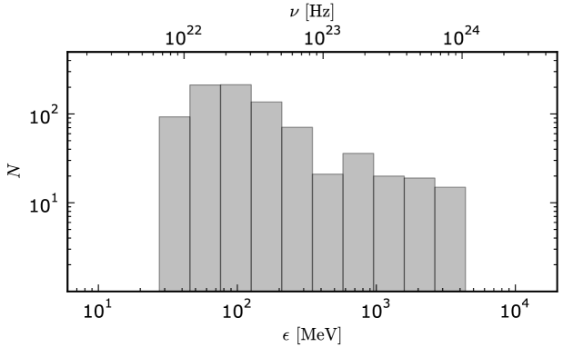
Figure 5.13: Distribution of ICS photons produced by an upscattering of warm spot radiation ($T_{{\rm s}}=1.0\,{\rm MK}$, $R_{{\rm ws}}=1\,{\rm km}$) for PSR B0834+06. The plot includes all $\gamma$-photons upscatterd by $50$ primary particles with Lorentz factors in the range of $2.5\times 10^{3}-10^{4}$.

5.2.1.3 Synchrotron Radiation

In both PSG-off and PSG-on modes SR plays a significant role in the generation of soft $\gamma$-ray photons. Figure 5.14 presents the places at which SR-photons are generated (left panel) and the SR spectrum (right panel) in the PSG-off mode for Geminga. The most energetic photons are generated close to the stellar surface ($z\approx 500\,{\rm m}$), while the less energetic ones are produced at altitudes $z>2\,{\rm km}$, where the magnetic field is weaker. SR in the PSG-off mode produces photons with energy in the range of from $30\,{\rm keV}$ to $1\,{\rm GeV}$. Again, the high energetic $\gamma$-photons produce electron-positron pairs in a strong magnetic field, thus its observation is not possible.

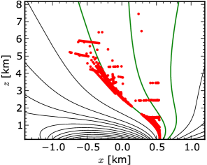
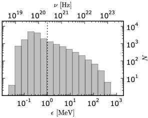
Figure 5.14: Synchrotron Radiation in the PSG-off mode for PSR J0633+1746. The left panel presents the places at which SR-photons are generated, while the right panel presents the SR-photons distribution. Plots were obtained in a cascade simulation calculated for a single primary particle moving along the extreme left open magnetic field line.

In Figure 5.15 we present the places of SR-photon generation (left panel) and the energy distribution of photons (right panel) in the PSG-on mode for Geminga.

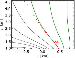
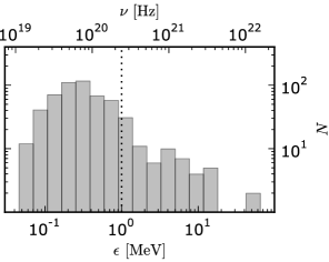
Figure 5.15: Synchrotron Radiation in the PSG-on mode for PSR J0633+1746. The left panel presents places at which SR-photons are generated, while the right panel presents the SR-photons distribution. Plots were obtained in a cascade simulation calculated for a single primary particle moving along the extreme left open magnetic field line. The ICS process was calculated using the whole surface radiation with temperature $T_{{\rm s}}=0.5\,{\rm MK}$ (see Table 1.4).

The production of SR-photons in the PSG-off mode starts at altitudes about $z\approx 1\,{\rm km}$ and ends at altitudes $z\approx 4.5\,{\rm km}$. Thus, the energy range of SR-photons is narrower, with the minimum and maximum photon energy $\epsilon_{{\rm min}}\approx 40\,{\rm keV}$ and $\epsilon_{{\rm max}}\approx 50\,{\rm MeV}$, respectively. Note the significant difference in the number of photons produced by SR in the PSG-off and PSG-on modes. The difference is a direct consequence of low secondary plasma multiplicity in the PSG-on mode (see Section 5.2.3).

5.2.2 X-ray emission

The main source of X-ray photons produced in the inner magnetosphere is SR. As mentioned in Section 5.2.1.1, to increase the amount of photons reaching the observer the emission zone should by located in the area with a weaker magnetic field. In this section we focus on the results of PSR B0943+10 and PSR 1929+10 for which the proposed configuration of a magnetic field satisfies this requirement (see Sections 2.4.4 and 2.4.7).

In the PSG-off mode most of the X-ray photons are produced by the SR of newly created electron-positron pairs. Figure 5.16 presents the final photon distribution produced by a single primary particle of PSR B1929+10 in the PSG-off mode. For a single primary particle we can estimate that only about $0.7\%$ of the total photon energy is in the range of $1-10\,{\rm keV}$. The bulk of the energy is carried away by newly created particles ($73\%$) and high energetic photons ($27\%$).

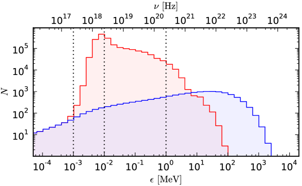
Figure 5.16: Final photon distribution produced by a single primary particle for PSR 1929+10 in the PSG-off mode. The blue line corresponds to the initial CR photons distribution, while the red line presents the final distribution with the inclusion of photon splitting, pair production and SR.

In Figure 5.17 we present the locations and the photon distribution of SR for PSR 1929+10 in the PSG-off mode. All SR-photons produced closer to the stellar surface will contribute to $\gamma$-ray emission, while the SR-photons produced at higher altitudes will produce photons in the X-ray band. As it results from Figure 2.26, the curvature at an altitude of $z\approx 3.5\,{\rm km}$ is only $50\%$ higher than at $z\approx 2\,{\rm km}$. Furthermore, before the particle reaches the region with a relatively low magnetic field ($z\approx 3.5\,{\rm km}$), it radiates a significant part of its energy at lower heights.

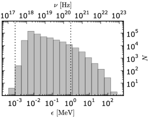
Figure 5.17: Synchrotron Radiation in the PSG-off mode for PSR B1929+10. The left panel presents the places at which SR-photons are generated, while the right panel presents the SR-photons distribution. Plots were obtained in a cascade simulation calculated for a single primary particle moving along the extreme left open magnetic field line.

To increase radiation in the $1-10\,{\rm keV}$ energy band we should apply the magnetic field structure with considerably higher curvature at altitudes where X-ray photons are generated. Although the curvature will not directly affect the SR, it will enhance CR, and thus it will increase the number of pairs produced in the region of a relatively weak magnetic field. In Figure 5.18 we present the final photon distribution produced by a single primary particle for PSR B0943+10 calculated using the magnetic field configuration as presented in Section 2.4.4.

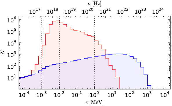
Figure 5.18: Final photon distribution produced by a single primary particle for PSR B0943+10 in the PSG-off mode. The blue line corresponds to the initial CR photons distribution, while the red line presents the final distribution with the inclusion of photon splitting, pair production and SR.

For this magnetic field structure about $3\%$ of the total photon energy is in the range of $1-10\,{\rm keV}$. The newly created particles carry away about $63\%$ of the energy radiated by the primary particle, while about $37\%$ of the energy remains in the form of photons.

The structure of the magnetic field of PSR B0943+10 allows enhanced pair production in a region of a weaker magnetic field (see Figure 5.19). The SR that accompanies pair production at higher altitudes ($z>3\,{\rm km}$) essentially increases the amount of energy radiated in the $1-10\,{\rm keV}$ energy band. Note, however, that the fraction of energy radiated in this band is still relatively low ($3\%$), and in order to be a substantial part of the observed X-ray spectrum the strong anisotropy of backstreaming and outstreaming plasma is required (see Section 5.1.3).

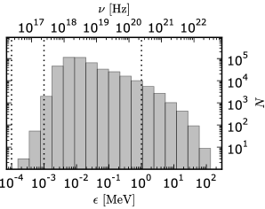
Figure 5.19: Synchrotron Radiation in the PSG-off mode for PSR B0943+10. The left panel presents the places at which SR-photons are generated, while the right panel presents the SR-photons distribution. Plots were obtained in a cascade simulation calculated for a single primary particle moving along the extreme left open magnetic field line.

In the PSG-on mode even for a complicated structure of the magnetic field most of the outflowing energy is converted to secondary plasma. Figure 5.20 presents the ICS-photons distribution produced in the PSG-on mode for PSR B0628-28. The bulk of energy is radiated in the form of high energetic $\gamma$-photons which are responsible for pair production, and thus the formation of secondary plasma. Taking into account not so high backstreaming/outstreaming anisotropy in the PSG-on mode, the ICS process is not relevant for the production of X-ray photons.

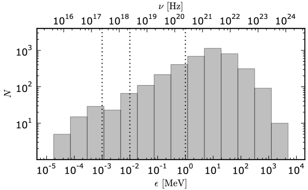
Figure 5.20: Distribution of ICS photons produced by an upscattering of the whole surface radiation ($T_{{\rm s}}=0.5\,{\rm MK}$) for PSR B0628-28. The plot includes all photons upscatterd by $50$ primary particles with Lorentz factors in the range of $3\times 10^{3}-1.2\times 10^{4}$.

The SR which accompanies the pair creation process in the PSG-on mode mostly produces soft $\gamma$-photons (see the right panel of Figure 5.21). Although the secondary pairs are produced at similar altitudes in both modes, (compare the left panels of Figures 5.19 and 5.21), the higher Lorentz factor of secondary plasma produced in the PSG-on mode results in higher energy of the SR-photons. The results suggest that when the gap operates in the PSG-on mode we should expect lower efficiencies of nonthermal X-ray emission than in the PSG-off mode. Note, however, that the final efficiency of X-ray radiation in the PSG-off mode highly depends on the backstreaming/outstreaming anisotropy and the structure of magnetic field lines.

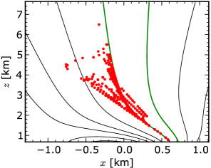
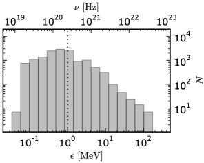
Figure 5.21: Synchrotron Radiation in the PSG-on mode for PSR B0628-28. The left panel presents places at which SR-photons are generated, while the right panel presents the SR-photons distribution. Plots were obtained in a cascade simulation calculated for $50$ primary particles with Lorentz factors in the range of $3\times 10^{3}-1.2\times 10^{4}$ moving along the extreme left open magnetic field line.

5.2.3 Secondary plasma

The multiplicity of secondary particles in the PSG-off mode is much higher than in the PSG-on mode. However, the primary plasma produced in the IAR of CR-dominated gaps has a density considerably lower than the Goldreich-Julian co-rotational density (see Equation 3.40). Figure 5.22 presents the energy histogram of secondary plasma for Geminga (left panel) and PSR B1133+16 (right panel). Despite major differences in the magnetic field structure and conditions in the IAR for both pulsars, the secondary plasma distribution shows many similarities. The only significant difference is the maximum Lorentz factor of secondary plasma, which for Geminga is about $\gamma_{{\rm sec}}^{{\rm max}}\approx 10^{4}$, while for PSR B1133+16 is is a few times smaller $\gamma_{{\rm sec}}^{{\rm max}}\approx 3\times 10^{3}$.

By using the overheating parameters presented in Table 3.1 we can roughly estimate that the final multiplicity of particles in the plasma cloud in the PSG-off mode ranges from $M=\kappa\cdot M_{{\rm sec}}\approx 2$ (for Geminga) to $M=\kappa\cdot M_{{\rm sec}}\approx 100$ (for PSR B1133+16). Note, however, that these values do not take into account the anticipated anisotropy of backstreaming and outstreaming particles. The existence of such an anisotropy could further increase the final multiplicity of particles in the plasma cloud leaving the inner magnetosphere. Despite the fact that without a full cascade simulation in the IAR we cannot unambiguously determine the final multiplicity in the plasma cloud, it can be clearly seen that depending on the details of the gap operating in the PSG-off mode, the produced plasma may be suitable (e.g. PSR B1133+16) or unsuitable (e.g. Geminga) to generate radio emission (see Section Radio emission). The main factor determining the parameters of the CR-dominated gap, and thus determining whether it is possible to effectively produce radio emission, is the radius of curvature of the magnetic field lines (see Section 3.3.2).

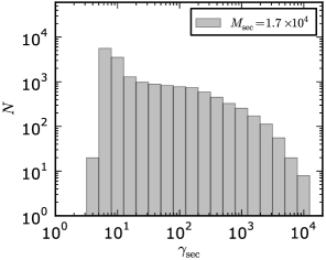
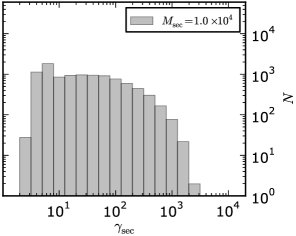
Figure 5.22: Energy histogram of secondary plasma in the PSG-off mode. The left panel was obtained in a cascade simulation calculated for a single primary particle moving along the extreme left open magnetic field line of PSR J0633+1746, while the right panel corresponds to a cascade simulation for PSR B1133+16.

In ICS-dominated gaps, on the other hand, the density of primary plasma produced in IAR exceeds the co-rotational density. Thus, the development of dense enough plasma for radio emission is much easier in the PSG-on mode. In Figure 5.23 we present the locations of pair production and energy distribution of secondary plasma in the PSG-on mode for PSR B0628-28. The final multiplicity of particles in the plasma cloud in the PSG-on mode can be calculated as $M=N_{{\rm ICS}}\times M_{{\rm sec}}$. As mentioned in Section 5.1.3, the exact value of $N_{{\rm ICS}}$ can be found only by performing the full cascade simulation in IAR but, as shown by Timokhin, (2010), we should expect a full screening of the acceleration region when $N_{{\rm ICS}}$ reaches a value as high as $20-100$. Thus we can roughly estimate that for the whole surface radiation with temperature $T_{{\rm s}}=0.3\,{\rm MK}$, the final multiplicity of secondary plasma in the PSG-on mode for PSR B0628-28 is of the order of $M\approx 100$.

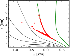
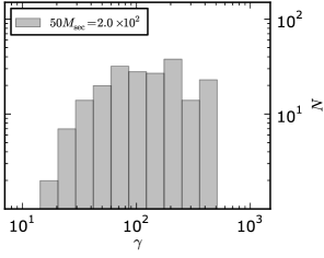
Figure 5.23: Secondary plasma produced in the PSG-on mode for PSR B0628-28. The left panel presents places at which pairs are produced, while the right panel presents the histogram of particle energy. Plots were obtained in a cascade simulation calculated for $50$ primary particles with Lorentz factors in the range of $3\times 10^{3}-1.2\times 10^{4}$ moving along the extreme left open magnetic field line. The ICS process was calculated using the whole surface radiation with temperature $T_{{\rm s}}=0.3\,{\rm MK}$.

In the PSG-on mode the main factor which determines the final multiplicity of secondary plasma is the source of the background photons. As shown in Section 4.4.4, the polar cap radiation (the hot spot component) has a negligible impact on the ICS process above the IAR. Figure 5.23 presents the location of pair production and energy distribution of secondary plasma for PSR B0628-28 calculated assuming the whole surface radiation with temperature $T_{{\rm s}}=0.5\,{\rm MK}$. The increase in the number of background photons results in enhancement of the ICS process, and thus an increase of the secondary multiplicity $M_{{\rm sec}}\approx 60$. For such conditions the final multiplicity of secondary plasma in the PSG-on mode is of the order of $M\approx 10^{3}-10^{5}$.

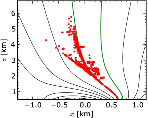
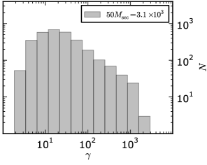
Figure 5.24: Secondary plasma produced in the PSG-on mode for PSR B0628-28. The left panel presents the places at which pairs are produced, while the right panel presents the histogram of particle energy. Plots were obtained in a cascade simulation calculated for $50$ primary particles with Lorentz factors in the range of $3\times 10^{3}-1.2\times 10^{4}$ moving along the extreme left open magnetic field line. The ICS process was calculated using the whole surface radiation with temperature $T_{{\rm s}}=0.5\,{\rm MK}$.

Conclusions

The hot spot component identified in X-ray observations implies the non-dipolar structure of surface magnetic field. We used the Partially Screened Gap model to explain both the X-ray radiation of radio pulsars and production of secondary plasma suitable for generation of radio emission.

A special case (PSR B0943+10)

Our model predicts two additional sources of X-ray emission: (I) the warm spot component and (II) enhanced SR radiation in the PSG-off mode. The warm spot component is associated with particles originating from the antipodal polar cap, while the high luminosity of X-ray photons produced in the PSG-off mode is a result of strong anisotropy of backstreaming and outstreaming particles.

Very recent results presented by Hermsen et al., (2013) show the anti-correlation of radio and X-ray emission of PSR B0943+10. The authors suggest an unpulsed, non-thermal component in radio-bright mode and a $100\%$-pulsed thermal component along with a nonthermal component in a radio-quiet mode. In our model it is not possible to produce an unpulsed, nonthermal X-ray component without the accompanying blackbody radiation of the polar cap. Although it is possible to produce nonthermal X-ray radiation which obscures the thermal component (strong SR in the PSG-off mode with a high predominance of outstreaming particles), the resulting radiation should be pulsed. We believe that the X-ray radiation of PSR B0943+10 in the radio bright mode was misinterpreted as the nonthermal one. As shown in Figure 1.7 (panel d), for a derived geometry of PSR B0943+10 the polar cap produces unpulsed, thermal radiation. Furthermore, as reported by the authors, in the radio-bright mode both the absorbed blackbody (BB) and the absorbed power-law (PL) models fit the spectrum equally well (see Table S4 in Hermsen et al.,, 2013). We believe that the observed radiation modes of PSR B0943+10 correspond to a mode switch between the PSG-on (radio-bright) and the PSG-off mode (radio-quiet). When pulsar is in the PSG-on we observe both the radio emission and thermal radiation which originates from the polar cap. In the PSG-off mode the secondary plasma is not suitable to produce so strong radio emission as in the PSG-on mode, but the polar cap radiation is accompanied by pulsed, nonthermal emission produced by SR (see Sec. 5.2.2).

Gamma-ray pulsars

As was shown in Sections 5.1.1 and 5.2.1, $\gamma$-rays produced in IAR and the inner magnetosphere cannot reach the observer due to efficient pair production in those regions. Current models of $\gamma$-ray emission propose that the emission comes from outer magnetospheric gaps. The non-dipolar structure of a magnetic field has two key implications on $\gamma$-ray emission models: (I) the formation of slot gaps is not possible as pairs are produced along all open magnetic field lines, (II) the high density of electron-positron plasma ($n_{p}\gg n_{{\rm GJ}}$) produced in the inner magnetosphere prevents the outer gap formation. The high-density plasma which crosses the null line will screen the outer magnetospheric region due to plasma separation (acceleration of electrons and deceleration of positrons). Thus, the formation of outer gaps is possible only in special cases when the pulsar operates in the PSG-off mode and produces secondary plasma with low density $n_{p}\approx n_{{\rm GJ}}$.

As recently reported by Arka and Dubus, (2013): “It is possible for relativistic populations of electrons and positrons in the current sheet of a pulsar’s wind right outside the light cylinder to emit synchrotron radiation that peaks in the ${\rm sub-GeV}$ to ${\rm GeV}$ regime, with $\gamma$-ray efficiencies similar to those observed for the Fermi/LAT pulsars.” We believe that the observed high-energetic $\gamma$-rays are produced in the not yet well explored region right outside the light cylinder.

Radio emission

Pulsed radio emission remains one of the most intriguing puzzles of astrophysics. It is remarkable that despite the large ranges in $P$, $B_{{\rm d}}$, the variations in the pulse profile between different classes of neutron stars (young, old, millisecond, magnetars) are similar to those within classes (Melrose,, 2004). The radio emission of most pulsars can be characterised by: a relatively narrow frequency range, $\sim 100\,{\rm MHz}$ to $\sim 10\,{\rm GHz}$, and a high degree of polarisation with a characteristic sweep of the position angle. The extremely high brightness temperature of pulsar radio emission (typically $T_{b}>10^{25}\,{\rm K}$) implies that a coherent emission mechanism is involved. Many radio emission mechanisms have been proposed, but no consensus on a specific emission mechanism has emerged. The radio observations alone cannot identify the emission mechanism and, hence, a model of the magnetosphere is needed to put constraints on the radio emission model. An acceptable emission mechanism must involve some form of instability to produce coherent radiation. The main difficulty in finding a specific emission mechanism is that many of the predicted features are common all proposed models. Furthermore, the polarisation can also be regarded as generic rather than associated with a specific emission mechanism (Melrose,, 2006).

The X-ray observations have allowed us to put constraints on the polar cap region of pulsars. The non-dipolar structure of the surface magnetic field causes plasma to form under similar conditions regardless of the global configuration of the magnetic field. We have showed that depending on the details of IAR, the resulting plasma either meets the requirements for efficient radio emission (suitable multiplicity and energy distribution of secondary plasma) or is not suitable to produce efficient radio emission (e.g. Geminga). Furthermore, the proposed drift model allows to find a connection between radio and X-ray emission processes (see Section 3.4).

The mixed mode

Although in the thesis we consider the PSG-on and PSG-off mode separately, in a real case both of these modes can coexist either on two separate polar caps or on the same polar cap occupying its different parts. In the latter case the change of modes is associated with varying degrees of intensity of the two modes. Furthermore, if specific conditions are met, the ICS process can be a main source of $\gamma$-photons in the lower parts of the gap, while the CR process can produce $\gamma$-photons in the upper parts of the acceleration region. In such a case distinguishing between the two modes is even more difficult.

Summary

The main propositions associated with this thesis are as follows:

1. The size of the hot spots implies that the magnetic field configuration just above the stellar surface differs significantly from a purely dipole one.

2. The analysis of X-ray observations shows that the temperature of the actual polar cap is equal to the so-called critical value, i.e. the temperature at which the outflow of thermal ions from the surface screens the gap completely.

3. The non-dipolar structure of a surface magnetic field and the high multiplicity of particles produced in IAR prevents the formation of slot and outer gaps.

4. The PSG model predicts the existence of two scenarios of gap breakdown: the PSG-off mode for CR-dominated gaps and the PSG-on mode for ICS-dominated gaps.

5. The two different scenarios of gap breakdown can in a natural way explain the mode-changing phenomenon when both modes produce plasma suitable to generate radio emission, and pulse nulling when the radio emission is not generated in one of the modes.

6. The mode changes of the IAR may explain the anti-correlation of radio and X-ray emission in very recent observations of PSR B0943+10 (Hermsen et al.,, 2013).

7. The regular drift of subpulses can be expected only when the gap operates in the PSG-on mode. The proposed model of drift allows to connect the drift information obtained by radio observations with the X-ray data of rotation-powered pulsars.

References

- Abdo et al., (2010) Abdo, A. A., Ackermann, M., Ajello, M., Atwood, W. B., Axelsson, M., Baldini, L., Ballet, J., Barbiellini, G., Baring, M. G., Bastieri, D., and et al. (2010). The First Fermi Large Area Telescope Catalog of Gamma-ray Pulsars. ApJS, 187:460–494.
- Abrahams and Shapiro, (1991) Abrahams, A. M. and Shapiro, S. L. (1991). Molecules and chains in a strong magnetic field - Statistical treatment. ApJ, 382:233–241.
- Adler, (1971) Adler, S. L. (1971). Photon splitting and photon dispersion in a strong magnetic field. Annals of Physics, 67:599–647.
- Arka and Dubus, (2013) Arka, I. and Dubus, G. (2013). Pulsed high-energy -rays from thermal populations in the current sheets of pulsar winds. A&A, 550:A101.
- Arons, (1993) Arons, J. (1993). Magnetic field topology in pulsars. ApJ, 408:160–166.
- Asgekar and Deshpande, (2001) Asgekar, A. and Deshpande, A. A. (2001). The topology and polarization of sub-beams associated with the ‘drifting’ sub-pulse emission of pulsar B0943+10 - II. Analysis of Gauribidanur 35-MHz observations. MNRAS, 326:1249–1254. [As01].
- Baade and Zwicky, (1934) Baade, W. and Zwicky, F. (1934). Remarks on Super-Novae and Cosmic Rays. Physical Review, 46:76–77.
- Backer, (1970) Backer, D. C. (1970). Correlation of Subpulse Structure in a Sequence of Pulses from Pulsar PSR 1919+21. Nature, 227:692–695.
- Baring et al., (2005) Baring, M. G., Gonthier, P. L., and Harding, A. K. (2005). Spin-dependent Cyclotron Decay Rates in Strong Magnetic Fields. ApJ, 630:430–440.
- Baring and Harding, (1997) Baring, M. G. and Harding, A. K. (1997). Magnetic Photon Splitting: Computations of Proper-Time Rates and Spectra. ApJ, 482:372–+.
- Baring and Harding, (2001) Baring, M. G. and Harding, A. K. (2001). Photon Splitting and Pair Creation in Highly Magnetized Pulsars. ApJ, 547:929–948.
- Baring and Harding, (2007) Baring, M. G. and Harding, A. K. (2007). Resonant Compton upscattering in anomalous X-ray pulsars. Ap&SS, 308:109–118.
- Baring and Harding, (2008) Baring, M. G. and Harding, A. K. (2008). Modeling the Non-Thermal X-ray Tail Emission of Anomalous X-ray Pulsars. In Y.-F. Yuan, X.-D. Li, & D. Lai, editor, Astrophysics of Compact Objects, volume 968 of American Institute of Physics Conference Series, pages 93–100.
- Baring et al., (2011) Baring, M. G., Wadiasingh, Z., and Gonthier, P. L. (2011). Cooling Rates for Relativistic Electrons Undergoing Compton Scattering in Strong Magnetic Fields. ApJ, 733:61.
- Becker, (2009) Becker, W. (2009). X-Ray Emission from Pulsars and Neutron Stars. In W. Becker, editor, Astrophysics and Space Science Library, volume 357 of Astrophysics and Space Science Library, page 91. [Be09].
- Becker and Aschenbach, (2002) Becker, W. and Aschenbach, B. (2002). X-ray Observations of Neutron Stars and Pulsars: First Results from XMM-Newton. In W. Becker, H. Lesch, & J. Trümper, editor, Neutron Stars, Pulsars, and Supernova Remnants, page 64. [Be02].
- Becker et al., (2005) Becker, W., Jessner, A., Kramer, M., Testa, V., and Howaldt, C. (2005). A Multiwavelength Study of PSR B0628-28: The First Overluminous Rotation-powered Pulsar? ApJ, 633:367–376. [Be05].