A distribution of large particles in the coma of Comet 103P/Hartley 2

Abstract

The coma of Comet 103P/Hartley 2 has a significant population of large particles observed as point sources in images taken by the Deep Impact spacecraft. We measure their spatial and flux distributions, and attempt to constrain their composition. The flux distribution of these particles implies a very steep size distribution with power-law slopes ranging from $-6.6$ to $-4.7$. The radii of the particles extend up to 20 cm, and perhaps up to 2 m, but their exact sizes depend on their unknown light scattering properties. We consider two cases: bright icy material, and dark dusty material. The icy case better describes the particles if water sublimation from the particles causes a significant rocket force, which we propose as the best method to account for the observed spatial distribution. Solar radiation is a plausible alternative, but only if the particles are very low density aggregates. If we treat the particles as mini-nuclei, we estimate they account for $<16-80$% of the comet’s total water production rate (within 20.6 km). Dark dusty particles, however, are not favored based on mass arguments. The water production rate from bright icy particles is constrained with an upper limit of 0.1 to 0.5% of the total water production rate of the comet. If indeed icy with a high albedo, these particles do not appear to account for the comet’s large water production rate.

Erratum: We have corrected the radii and masses of the large particles of comet 103P/Hartley 2 and present revised conclusions in the attached erratum.

1 Introduction

Comet 103P/Hartley 2 (hereafter, 103P or Hartley 2) is a hyperactive comet. The activities of most comets are consistent with surfaces that are over 90% inert, i.e., activity is restricted to a few localized sources. In contrast, the gas production rates of the hyperactive comets suggest activity over $\sim 100$% of their surfaces or more. Comet Hartley 2’s peak water production rate during the 1997 perihelion passage was $Q_{H_{2}O}\approx 3\times 10^{28}$ molec s^-1 (Combi et al. 2011). The sublimation rate of an isothermal nucleus with a 4% Bond albedo at 1.03 AU (the 1997 perihelion distance of Hartley 2) is $2.9\times 10^{17}$ molec cm² s^-1 (Cowan and A’Hearn 1979). Thus, approximately 10 km² of surface area would be required to match the measured water production in 1997. However, constraints on the size of the nucleus by Groussin et al. (2004) and Lisse et al. (2009) suggested the total surface area was near 4–6 km², yielding an active fraction (area based on $Q_{H_{2}O}$/area of the nucleus) near 1.7–2.5. In order to account for the high active fraction, Lisse et al. (2009) proposed that the coma contained a population of icy grains, which increased the surface area available for sublimation, and therefore allowed for a relatively high water production rate.

The Deep Impact spacecraft flew by Comet 103P on 4 November 2010. The minimum flyby distance was 694 km, occurring at 13:59:47.31 UTC with a relative speed of 12.3 km s^-1 (A’Hearn et al. 2011). Rather than just being the fifth comet nucleus to be imaged up close by a spacecraft, Comet Hartley 2 might also be considered an archetype of the hyperactive comets. The flyby images verified the small surface area of the nucleus (5.24 km²; Thomas et al. this issue), and Deep Impact’s IR spectrometer revealed a coma of icy grains (A’Hearn et al. 2011). Knight and Schleicher (this issue) discovered tail of OH and NH, evident on $10^{4}$ km scales, which they conclude are derived from small grains of ice that were accelerated down the tail before completely sublimating. Bonev et al. (this issue) observed enhanced heating of the water gas 20–150 km down the tail, which they also attribute to sublimating ice grains in the tail. The icy coma hypothesis of Lisse et al. (2009) seems to be qualitatively valid. What remains is a quantitative verification that the ice grains in the coma are a significant source of water gas.

A’Hearn et al. (2011) also discovered bright point sources distributed around the nucleus of Hartley 2 in visible wavelength images. The fluxes of these sources are consistent with a population of objects centimeter-sized or larger. A’Hearn et al. (2011) could not determine if these large particles were icy or refractory. In the following paper, we will attempt to discern the nature of these point sources and if they might be the cause of Hartley 2’s hyperactivity.

The point sources around Hartley 2 are found in visible wavelength images taken with both the High Resolution Instrument (HRI) and the Medium Resolution Instrument (MRI). Their spatial distributions and densities vary, but they are not background stars; celestial sources are significantly streaked in images taken while the spacecraft-comet distance, $\Delta$, was less than $10^{4}$ km. That the HRI detected these point sources is significant. The HRI visible camera (HRIVIS) is not in optimal focus, and has an accordingly large and doughnut-shaped point spread function (PSF) (Lindler et al. 2007). Thus, unresolved sources are easily discriminated from cosmic ray impacts and hot pixels. None of the point sources appear to be resolved, therefore they must be smaller than the FWHM of the HRIVIS deconvolved PSF (approximately 3 m at $\Delta=700$ km).

In addition to point sources, streaks of various lengths are present in many of the images. The lengths of the streaks are correlated with exposure time (longer exposures produce longer streaks), and inversely proportional to instrument pixel scale (streaks in HRIVIS images are longer than in MRI). The streaks are parallel to each other, and the orientation is consistent with the spacecraft’s motion as it tracks 103P’s nucleus. Stars and other distant objects produce streaks of uniform length and orientation, but we find a variety of streak lengths in a single image, down to a few pixels long, which indicates they are spatially close to the nucleus and not celestial sources.

Altogether, the above observations indicate that the nucleus of Comet 103P is surrounded by a coma of thousands of large particles. We will use the term “particle” to refer to the observed point sources in this paper. A’Hearn et al. (2011) demonstrated that these particles are centimeter-sized or larger. Large particles are not unique to this comet, but these observations are unique to large particles. These are the first images of sub-meter particles from a comet seen as individual objects. Prior images in visible/infrared light (e.g., comet dust trails; Sykes and Walker 1992, Ishiguro et al. 2002, Reach et al. 2007) and with radar (Harmon et al. 2004) probed collections of many large particles. The only other observations of large individual particles from comets that we can think of are those of meteors (from meteor streams associated with particular comets) and milligram particle impacts on spacecraft. Although the latter examples may only be of order 0.1–1 mm in size.

In the following paper, we present our methods for detecting and measuring the photometric properties of the large particles in the coma of Comet 103P. We will convert their fluxes into sizes, discuss their spatial distribution, attempt to constrain their composition, and compare them to large particles observed in radar observations of the comet. Assuming they are icy, we also constrain their contribution to the comet’s total water production rate.

2 Observations

Images of Comet 103p Were taken with Deep Impact’s Medium Resolution Instrument and High Resolution Instrument CCD cameras. Both cameras have $1024\times 1024$ pixel arrays; the HRIVIS pixel scale is 0.413^′′ pixel^-1 (2 µrad), and the MRI pixel scale is 2.06^′′ pixel^-1 (10 µrad). The instruments are described by Hampton et al. (2005), and their calibration by Klaasen et al. (2008, in prep.). The MRI and HRIVIS data are available in the NASA Planetary Data System (PDS) archive (McLaughlin et al. 2011a, b). Images taken with the MRI are labeled with the prefix mv, and for the HRIVIS the prefix is hv. We keep this convention throughout the paper. We used a pre-PDS data set, but the only significant difference is the absolute flux calibration constant, which we account for in our photometry.

Optimal focus for the HRIVIS instrument occurs about 6 mm before the focal plane. For this instrument, it is often beneficial to work with spatially restored (i.e., deconvolved) images. We follow the method of Lindler et al. (2007), using the HRIVIS PSF from the EPOXI mission (Barry et al. 2010), to restore raw HRIVIS images to near diffraction-limited resolution. The HRIVIS images are deconvolved (Fig. 6b) with the Richardson-Lucy (R-L) method modified to handle non-Poisson CCD readout noise (Snyder et al. 1993, Lindler et al. 2007). Note that R-L restoration methods conserve flux.

The large particles are easily seen in MRI and HRIVIS images at $\Delta\lesssim 10^{4}$ km. Outside of this range, the particles become increasingly faint, overwhelmed by the diffuse coma’s surface brightness, and confused with stars, which are unstreaked point sources when the spacecraft-comet distance is large. In a manual search, the earliest image in which we have identified particles is HRIVIS image hv5000096, taken 22,400 km from the nucleus (CA-30 min, 1500.5 ms exposure time). The first MRI image in which we have positively identified particles is mv5002025 (8580 km, CA-11 min, 500.5 ms).

Most images at $\Delta<10^{4}$ km use the CLEAR1 filter. For sources with solar-like spectra, the CLEAR1 filters have effective wavelengths of $\lambda_{e}=0.625$ µm for HRIVIS, and 0.610 µm for MRI, and a FWHM of $\approx 0.5$ µm. The absolute calibration uncertainties for the CLEAR1 filters are 5% for HRIVIS, and 10% for MRI (Klaasen et al. 2008). Large particles have not yet been identified in the HRI infrared spectrometer (HRIIR) scans (Protopapa et al. 2011), but they may be discovered in the future when we can predict the location of the brightest particles in IR data using their MRI and HRIVIS derived 3D positions and velocities (Hermalyn et al. this issue).

A summary of all images used in this paper is presented in Table 1. Note that the HRIVIS images used in this paper are only a small sub-set of the HRIVIS particle observations. We have limited our investigation to the closest-approach images because of the great amount of time that must be taken to analyze the HRIVIS data. We also do not use any of the 50.5 ms MRI images in the PDS archive. These images were taken along with the 500.5 ms images, but few particles are found in these images due to the decreased sensitivity and great distances from the nucleus.

3 Detection, photometry, and completeness

3.1 MRI images

We automatically detect and measure all point sources throughout all MRI images taken within $\Delta<5200$ km of the comet nucleus using DAOPHOT as included in the IRAF software package (Tody 1993). In summary, we: (1) estimate the PSF of the instrument and verify that it accurately measures particle fluxes; (2) remove the diffuse coma from the images; (3) mask the nucleus and bright jets; (4) additionally mask stars in images at large $\Delta$; (5) measure the completeness of our particle census (i.e., detection efficiency); (6) estimate the photometric uncertainties, and correct for any biases; and, (7) clean bad PSF fits and crowded regions from our photometry lists. Below, we provide details on our methods.

Particles were detected by searching for point sources (FWHM $=1.5$ pixels) with a peak amplitude greater than $5\sigma$ above the local background: $1\sigma$ per pixel $\approx 1.1\times 10^{-3}$, $0.52\times 10^{-3}$, and $0.13\times 10^{-3}$ W m^-2 µm^-1 sr^-1 for 41, 121, and 501 ms frames, respectively. Twenty-five isolated and bright point sources were selected by hand from image mv5004056 to estimate the MRI PSF. The sources were fit by DAOPHOT with a variety of functions, and the best-fit PSF used a Moffat function ($\beta$ parameter of 1.5; Moffat 1969) with a look-up table of empirical residuals. We compared DAOPHOT-derived fluxes of bright isolated particles to those measured with aperture photometry. The values agreed, with a mean error of $\Delta F_{\lambda}/F_{\lambda}=-1.9\%$, where $\Delta F_{\lambda}$ is the difference between the DAOPHOT flux and the aperture flux ($F_{\lambda,\rm DAOPHOT}-F_{\lambda,\rm aper}$).

DAOPHOT iteratively estimates the background as it fits each point source and groups of point sources, but we found—especially for detections closer to the nucleus—that subtracting an initial estimate of the background improved DAOPHOT’s ability to find and measure sources. Furthermore, the MRI CCD has an instrumental background that varies row-by-row at the 1–4 DN level (the MRI and HRIVIS calibration constants for CLEAR1 are $3.527\times 10^{-5}$ and $1.209\times 10^{-4}$ W m^-2 µm^-1 sr^-1 DN^-1 s, respectively). The EPOXI pipeline includes a routine to detect and remove this background, but it is not executed on images dominated by coma, such as those in our analysis. We derive our background estimate for each image using two median filters (i.e., low-pass filters). We first apply a $3\times 25$ pixel (row $\times$ column) filter that defines the background stripes, as well as much of the coma. A second $25\times 3$ pixel filter defines most of the residual coma, especially where it is extended along image columns. A median-filter subtracted image is presented in Fig. 1b.

Bright jets and the nucleus complicate the PSF fitting. Therefore, we mask these regions on the image. The mask is derived from a morphological gradient with an $11\times 11$ pixel uniform structuring element, which effectively generates an image of peak-to-peak values in a moving $11\times 11$ pixel box (Fig. 1c). We threshold the gradient image at a value of 0.1 W m^-2 µm^-1 sr^-1, then dilate the mask by 30 pixels to fill small gaps between features, and cover some of the nearby jets (Fig. 1d).

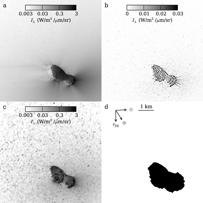
Figure 1: The process by which we remove the background and mask the nucleus in MRI images. (a) A fully calibrated image, mv5004046. (b) The median-filter subtracted image. (c) Image of the morphological gradient of image b. (d) The final mask, defined where image c $>0.1$ W m^-2 µm^-1 sr^-1. The mask has been dilated by 30 pixels to fill gaps and cover some additional coma. The image scale and orientation are given in panel d. The projected vectors are comet-Sun ($\odot$), comet-Earth ($\oplus$), and spacecraft velocity ($v_{\rm DI}$).

DAOPHOT will occasionally fit streaks in the MRI images with PSFs. Most of these fits have poor residuals, and are removed before the final analysis (described below). But we found several streaks persisting into the final analysis in images taken at large distances from the comet ($\Delta\gtrsim 5000$ km). These streaks were stars and not particles. DAOPHOT seemed more likely to fit streaks in these images because the stars are much brighter than the particles, and are only streaked several pixels or less. We generated an additional mask by searching for elongated sets of pixels above the background in order to remove streaked celestial objects from these images before processing with DAOPHOT. At closer comet-spacecraft distances, stars are streaked over a greater number of pixels (up to a few hundred pixels at closest approach), and are easily rejected without the mask.

We verified the completeness (i.e., detection efficiency) of our method by inserting artificial point sources into each image, re-executing our scripts on the new images, and examining the output to determine if the artificial sources were detected. The completeness is then the fraction of detected artificial sources per flux bin. We inserted 1% of the number of detected point sources (with a minimum of 10 new particles) uniformly over the image but avoiding the nucleus. The fluxes were picked from a distribution uniform in log-space, based on the minimum and maximum fluxes measured in the image. The process is repeated, each time starting with the original image, until 3000 artificial particles have been tested. Examples of our MRI completeness test results are shown in Fig. 2. The completeness is directly correlated with exposure time; in general, it is easier to find and measure fainter particles in images with longer exposures. In our MRI population studies, we will only consider particles brighter than the 80% completeness level for each image (listed in online Table LABEL:tab:fits as $F_{\lambda,{\rm min}}$).

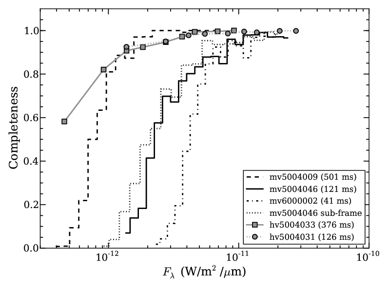
Figure 2: Example point source detection completeness functions. All images were taken within $\Delta=694-704$ km, except mv5004009 (501 ms) taken at $\Delta=1858$ km. The mv5004046 sub-frame is chosen to match the same area as covered in hv5004031. The HRIVIS test particles are selected from one of 9 specific fluxes (marked by squares and circles), whereas the MRI test particles are selected at random from a range of fluxes. The lowest of the HRIVIS bins is 10,000 e^-.

The completeness tests can be used to derive the photometric uncertainties. As an example, we plot the input flux versus the DAOPHOT flux error for all artificial particles added to image mv5004046 (Fig 3). In this image, the mean flux error $\overline{\Delta F_{\lambda}/F_{\lambda}}=-8\%$, and the mean error for all images ranges from $-10$% to $-2$%. However, the distribution is not Gaussian as there is a significant tail at large negative errors. If we instead take the resistant mean (clipping at $3\sigma$), we find the mean $\Delta F_{\lambda}/F_{\lambda}$ ranges from $-3.5$% to $-0.7$%, with per image standard deviations ranging from 6% to 10%. As discussed above, we also found a slight negative error when we compared the DAOPHOT photometry to aperture photometry of isolated bright sources. To account for this effect, we will increase the fluxes of all particles by 2%. In addition, we adopt 8% as our particle flux uncertainty.

The large flux errors ($|\Delta F/F|>10\%$) are likely misidentified artificial particles, artificial particles that have merged with brighter particles in the PSF fitting process, and PSF over/under fitting. Any particles with significantly large flux errors must be identified and removed from our photometry lists so that they do not affect the final results. We clean the DAOPHOT output by rejecting: (1) bad PSF fits as identified by DAOPHOT (i.e., reduced $\chi^{2}>2.0$); and (2) any particles with a total residual in a $3\times 3$ pixel box greater than $3\sigma$ from the background. For the 41 ms images $62-78\%$ and $0-2\%$ of the detected sources were rejected by the two criteria, respectively. For the 121 ms images the rejection rates were $5-32\%$ and $2-5\%$; for 501 ms, the rates were $0-1$%, and $3-20$%. Occasionally DAOPHOT fits portions of the particle streaks, and these criteria help remove such spurious fits from the photometry lists. Examples of point source cleaned images are shown in Figs. 4 and 5. After point source cleaning, sources not fit by DAOPHOT are evident. These particles can be accounted for in a statistical sense with the image’s completeness function, e.g., when we are displaying the flux distribution of the particles, we divide the measured flux distribution by the completeness curve to show the true flux distribution.

In Fig 5 we specifically show a region of high point source density, and the large number of bad-PSF fits resulting from point source crowding near the nucleus ($>0.025$ pixel^-1). These sources are primarily rejected by the $\chi^{2}$ criterion. Regions with a rejection rate $>20\%$ in a $25\times 25$ pixel area will be masked from our analyses.

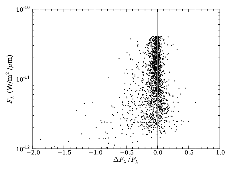
Figure 3: Input flux, $F_{\lambda}$, plotted versus DAOPHOT error, $\Delta F_{\lambda}/F_{\lambda}$, for all artificial particles inserted in image mv5004046. Most fluxes are measured to within 8% ($1\sigma$) of their true value, with a slight skew toward negative errors.

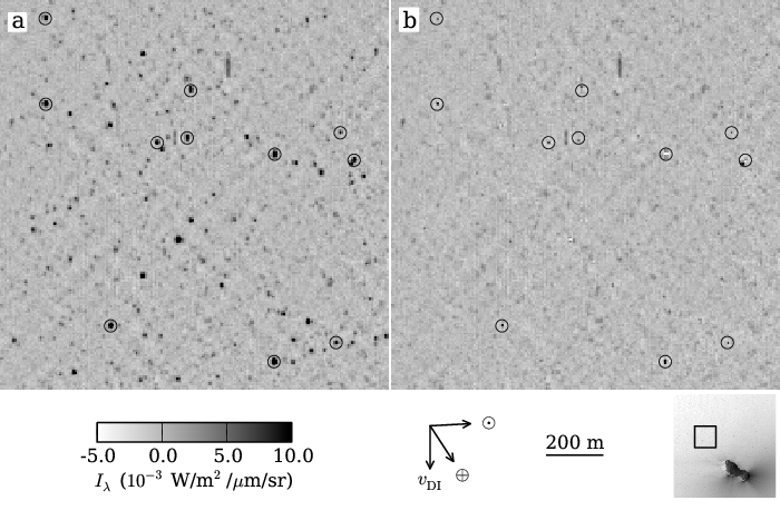
Figure 4: (a) A detail of image mv5004046, after background coma subtraction. (b) The same image after being cleaned of point sources detected and fit by DAOPHOT. In both images, particles with large residuals or low signal-to-noise flux ratios have been circled. Similar to Figure 1, the image scale and orientation are shown. The square in the lower right image shows the field of view of panels a and b with respect to the nucleus.

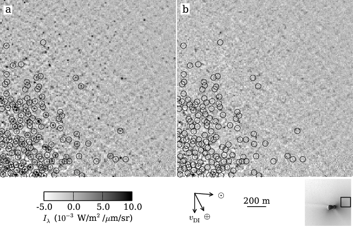
Figure 5: The same as Fig. 4, but for a region of high point source density in image mv5004029.

3.2 HRIVIS images

The analysis of the HRIVIS images required an approach independent from the MRI analysis. Figure 6a shows an HRIVIS image of the large particles and Fig. 6b is the restored (i.e., deconvolved) image. The broad defocused PSF and the longer trails resulting from parallax motion make PSF fitting even more difficult than in the MRI images. Our approach is to instead detect and measure a particle’s brightness in restored images. In summary, we: (1) iteratively remove the background from each image; (2) detect point sources and streaks in the restored images; (3) measure particle fluxes; and, (4) measure the completeness of our particle detection scheme. Below we detail our methods.

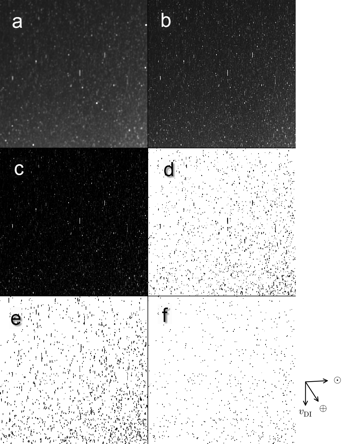
Figure 6: (a) Original HRIVIS image hv5004030. (b) Image deconvolved with the R-L method. (c) Image b after background subtraction. (d) Mask of pixels greater than 1000 e^- above the background. (e) Mask of detected sources. (f) Mask of the sources used to compute the flux distribution slope (here, length 5 pixels or smaller and total flux greater than 20,000 e^-).

We use an iterative technique to remove the background before final object detection and photometry. The initial background is set to the deconvolved image filtered with a $51\times 51$ pixel median filter. We then fit a smooth surface (using cubic splines) to the filtered image to obtain our background image. The objects within the image will bias the median filter and the resulting image overestimates the background. To minimize this bias, we repeat the process after ignoring all pixels more than 400 e^- above the background (object pixels) during median filtering (1 e^- s^-1 = $4.32\times 10^{-6}$ W m^-2 µm^-1 sr; Klaasen et al. in prep.). We repeat this process three times to obtain and remove our final background (Fig. 6c).

We detect the objects in the image by creating a mask of all pixels more than 1,000 e^- above the background level (Fig. 6d). We selected the 1,000 e^- threshold by visual inspection of the restored image to avoid detection of restoration artifacts that result from “ringing” around the brighter objects (Lindler et al. this issue). We define contiguous masked pixels as part of the same object. Visual inspection of this mask shows many instances where a trailed particle near the detection threshold is split into multiple objects because of noise and potential variations in particle brightness during the time of the exposure. To avoid this problem, we examine each detected object (starting with the brightest) and adding all pixels within a factor of 3 of the brightest pixel in the object. We define the resulting contiguous dark regions as our detected objects (Fig. 6e).

We perform photometry on the detected particles by starting with the particle mask, and adding the flux from their nearest-neighbors (i.e., we grow the mask by 1 pixel, and sum the pixels together). Non-linearities are a concern when restoring an image with non-linear deconvolution algorithms (Lindler et al. 1994). Fainter point sources will be broader than brighter point sources in a restored image. We can minimize any non-linearities by increasing the size of the region used for photometry. However, this results in more contamination of our results by nearby sources. To test for non-linearity we increased the size of the photometry regions by adding additional neighbors (i.e., including next-nearest neighbors, etc.). These larger regions showed that non-linearity artifacts are absent from particles brighter than 10,000 e^- ($F_{\lambda}=1.4\times 10^{-12}$ and $4.6\times 10^{-13}$ W m^-2 µm^-1 for exposure times of 126 and 376 ms). On average, the effective aperture for point sources is approximately a 3 pixel radius circle.

As done with the MRI analysis, we measure the completeness by inserting artificial objects in the images of varying brightness and parallax length. These artificial objects are added to the raw images before deconvolution. The completeness test also gives additional evidence that our measured fluxes are linear with object brightness in the range of brightness being considered. For the longer trails, the completeness decreased rapidly with flux. We therefore decided to ignore particles with a length more than 5 pixels in the restored image. In effect, this criterion limits the line-of-sight distance of the particles from the nucleus to $<1-2$ km at closest approach ($\Delta=694$ km), and $<2-3$ km at $\Delta=900$ km. If the flux distribution is independent with distance from the nucleus, then the relative distribution of number versus flux will remain unchanged. Limiting the length of the objects also has added benefits. Long streaks are much more likely to be a combination of multiple particles and their photometry is also more strongly affected by errors in the background estimation (they cover more pixels). Examples of our HRIVIS completeness test results are presented in Figure 2. There is little difference between the 126 ms and 376 ms completeness curves in the example. Therefore our completeness is not as strongly affected by background noise as it is by other factors, e.g., point source crowding and deconvolution artifacts. In addition, our HRIVIS photometry is generally limited by the linearity criterion of $F>10,000$ e^-.

4 Particle fluxes

4.1 Flux distribution

We measure the fluxes of all particles and compute their flux distributions, $dn/dF$. The particle fluxes approximately follow a power-law distribution. Therefore, we fit each flux distribution with a function of the form $dn/dF\propto F^{\alpha}$ using the method by Clauset et al. (2009), which is based on Kolmogorov-Smirnov tests and maximum likelihood fitting. We restricted the flux range to particles brighter than our 80% completeness estimate. This restriction increases the statistical errors in the fits but reduces possible bias errors resulting from photometry contamination from neighboring particles and residual background. Moreover, the fitting method does not include a correction for completeness, so restricting the fluxes helps mitigate the effect of incomplete counting; the maximum completeness correction over our fit range is 20%, which is insignificant in comparison to the strong power-law slopes (see Fig. S6 of A’Hearn et al. 2011). Our results are listed in Table LABEL:tab:fits and summarized in Table 3. In Figs. 7 and 8, we plot the final flux distributions and their best-fit trends. The fluxes are plotted as a function of $\mbox{$F_{\lambda,700}$}\equiv F_{\lambda}\Delta^{2}/700^{2}$ so that they may be directly compared to each other (variation of the phase angle is small, ranging from 79 to 92^∘, and is therefore not considered). The error-weighted mean slopes for the MRI and HRIVIS frames are $-3.74\pm 0.02$ and $-2.85\pm 0.03$, respectively.

The MRI and HRIVIS slopes are significantly different from each other. To verify this difference, we also computed the flux distributions from MRI sub-frames of images chosen close in time to the HRIVIS images. The relative position of the HRIVIS and MRI fields are constant with time, therefore measuring the flux distribution in the same field of view is straightforward. The comparison, however, is not exact because the frame-to-frame parallax of individual particles can be significant (Hermalyn et al. this issue). After bad-PSF rejection and completeness tests only $\approx 130$ particles could be used to determine the flux distributions in the MRI sub-frames. This is a factor of 3–10 fewer than the number of particles in the HRIVIS images. The difference primarily relies on the larger aperture of the HRI primary, which allows for a fainter point source detection limit due to the finer resolution and greater light gathering area. Our best-fit parameters for the MRI sub-frames are listed in Table LABEL:tab:fits and summarized in Table 3. The uncertainties in the power-law slopes are quite large, ranging from 0.18 to 0.31, owing to the paucity of particles available in the MRI sub-frame images. The weighted mean slope is $-3.59\pm 0.07$, which is shallower than the mean MRI full-frame slope, but they agree at the $2\sigma$ level.

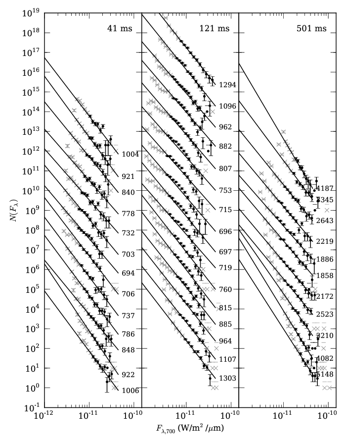
Figure 7: Flux distributions ($dn/d\log{F}$) and their best-fit power-law functions for all full-frame MRI data sets listed in Table LABEL:tab:fits. The flux distributions have been corrected for completeness, and their error bars are based on Poisson statistics. The flux distributions are grouped by their integration times, and sorted by time with the pre-closest approach images at the bottom. Each $i$-th flux distribution ($i=0,1,\ldots$) has been offset along the y-axis by $10^{i}$, and labeled with $\Delta$ for clarity. Additionally, the fluxes have been scaled by $(\Delta/700)^{2}$ so that they are directly comparable to each other. The gray $\times$ symbols mark particles not used in the fit.

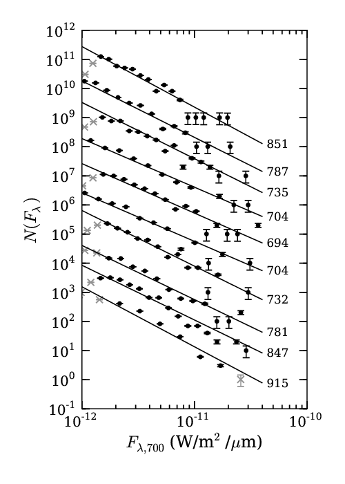
Figure 8: Same as Fig. 7, but for all HRIVIS images listed in Table LABEL:tab:fits.

Taken together, the mean MRI full-frame, MRI sub-frame, and HRIVIS best-fit power-law slopes show evidence that the flux distribution steepens with increasing flux. Inspection of the MRI full-frame distributions in Fig. 7 and the Kolmogorov-Smirnov probability ($P_{KS}$) values reveals that a power-law size distribution is not a good fit to most of the flux distributions. This poor fit is especially true for the 121 ms frames at $\Delta<900$ km where there is a significant curvature in the log-flux distributions of these images. The curvature is non-existent or not prevalent in the shorter exposure MRI data, the distant MRI data ($\Delta>1000$ km), and the HRIVIS data.

It is important to recognize two points. First, the HRIVIS distributions are poorly populated at $\mbox{$F_{\lambda,700}$}>10^{-11}$ W m^-2 µm^-1, whereas the 121 ms MRI distributions are well defined up to $\mbox{$F_{\lambda,700}$}\approx 3\times 10^{-11}$ W m^-2 µm^-1. This difference is simply a matter of the larger solid angle observed by the MRI camera as compared to the HRIVIS camera; a larger solid angle allows for more of the brightest particles to be detected. Second, the HRIVIS distributions are valid to lower fluxes than the MRI distributions (column $F_{\lambda,{\rm min}}$ in Table 3), because the larger primary of the HRI allows for fainter particles to be accurately measured. Taken together, these differences demonstrate that the two instruments are measuring two different particle flux regimes. In Fig. 9, we plot our best-fit power-law slopes versus the minimum flux used in each fit. A trend is evident; steeper slopes are correlated with larger $F_{\lambda,{\rm min}}$, but due to the different techniques, fit uncertainties, and fields of view involved, the correlation is not conclusive. We remind the reader that the correlation is not due to incomplete photometry because we restricted our data sets to fluxes where the completeness is better than 80%. Given this restriction, none of our completeness corrections are strong enough to have a significant effect on the best-fit slopes.

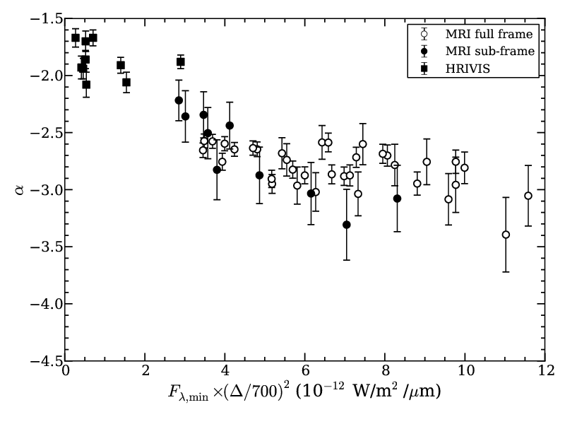
Figure 9: Best-fit power-law slope versus minimum flux used in the fit for all images listed in Table LABEL:tab:fits.

In the absence of any additional information on the flux distribution we will proceed assuming that the differences between the MRI and HRIVIS flux distributions reflect the true flux distribution of the entire particle population. As alternatives to a power-law distribution, we also considered a power-law with an exponential cut off, and a double power-law. The functional forms are

$$\frac{dn}{dF} \propto F^{\beta_{1}}\exp{(-F/\gamma_{1})}\mbox{ ,}$$ (1)

$$\frac{dn}{dF} \propto\frac{F}{\gamma_{2}}^{\beta_{2}}\left(1+\frac{F}{\gamma_{2}}\right)^{\beta_{3}-\beta_{2}}\mbox{ ,}$$ (2)

where $\beta_{i}$ are power-law slopes, and $\gamma_{1}$ is the flux at which the exponential decay reaches a factor of $\exp{(-1)}=0.37$ , and $\gamma_{2}$ is the turn-over flux from the low- to the high-flux slopes (both $\gamma$ parameters are specified for $\Delta=700$ km). The double power-law fits did not converge on a single solution. The power-law with exponential cut-off function, however, is a better fit to the closest-approach data ($\Delta<1000$ km), with a mean slope and cut-off equal to $-3.18\pm 0.07$ and $(5.7\pm 0.3)\times 10^{-12}$ W m^-2 µm^-1. Unfortunately, these best-fit values are poor fits at larger distances where the flux distribution better agrees with a power-law (Fig. 10). We suggest that the 121 ms distributions have a systematic effect that causes under-counting of the largest flux bins. Again, we note that our completeness corrections are not strong enough to significantly affect our fits, and that the distributions as shown in Figs. 7 and 10 have been corrected for completeness, yet the curvature remains in the closest approach data.

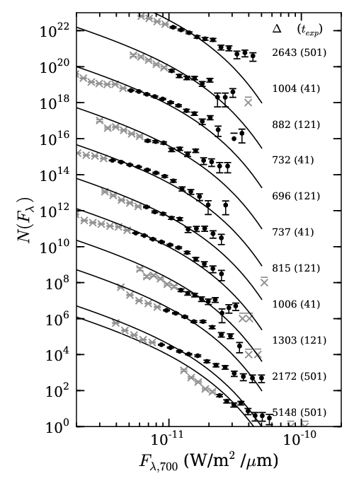
Figure 10: Best-fit power-law with exponential cut off, derived from 121 ms MRI images taken within $\Delta=1000$ km, compared to selected flux distributions, labeled with “$\Delta$ (exposure time)” in km and ms. The histograms have been offset by a factor of $10^{i}$ for clarity.

To test the hypothesis that the power-law slope is affected by the source density, we generated completely synthetic data sets with DAOPHOT, based on our MRI PSF. We created 8 images each with the same power-law flux distribution ($dn/dF\propto F^{-3.5}$) and maximum point source flux ($\mbox{$F_{\lambda,{\rm max}}$}=1\times 10^{-10}$ W m^-2 µm^-1), but $F_{\lambda,{\rm min}}$ varied from $5\times 10^{-12}$ down to $1.5\times 10^{-13}$ W m^-2 µm^-1. We inserted the same number of point sources per logarithmic flux bin, but because each image’s flux distribution spanned a different range, the total point source density varied from $4\times 10^{-4}$ pixel^-1 up to 2.6 pixel^-1. We then measured each image’s flux distribution with DAOPHOT in a manner similar to our MRI images. Once the input column density reached 0.08 pixel^-1, our best-fit slopes steepened from the input $-3.5$ down to a minimum of $-4.7$ at the highest densities. Thus, the rollover in the flux distribution seen in the 121 ms MRI images at $\Delta<1200$ km could be a manifestation of this effect.

The slopes derived from the distant MRI and the 41 ms MRI images are consistent: $\alpha=-3.80\pm 0.02$ and $-3.83\pm 0.05$, respectively. They agree despite the wide range in the number of particles fit (100–1000) and spacecraft-comet distances (900–5000 km, although the best constraints are within 3000 km). Therefore, we consider these results to be robust and representative of the true flux distribution for $\mbox{$F_{\lambda,700}$}\gtrsim 1\times 10^{-11}$ W m^-2 µm^-1. The shallower HRIVIS slopes appear valid for $1\times 10^{-12}\lesssim F_{\lambda}\lesssim 1\times 10^{-11}$. We see no reason to trust one data set over the other, or to assume that a single power-law would be valid for all fluxes measured. Therefore, we will use a broken power-law for the remainder of the paper:

$$\frac{dn}{dF}\propto F^{\alpha}\begin{cases}\alpha=-2.85&\text{ for }\mbox{$F_{\lambda,700}$}<7.2\times 10^{-12}\text{ W~{}m${}^{-2}$~{}\mbox{\textmu{}m}${}^{-1}$}\\ \alpha=-3.80&\text{ for }\mbox{$F_{\lambda,700}$}\geq 7.2\times 10^{-12}\text{ W~{}m${}^{-2}$~{}\mbox{\textmu{}m}${}^{-1}$}\\ \end{cases},$$ (3)

where $\mbox{$F_{\lambda,700}$}=7.2\times 10^{-12}$ is the break in the power-law, $-2.85\pm 0.02$ is the average HRIVIS slope, and $-3.80\pm 0.02$ is the average MRI slope, measured from images at $\Delta>900$ km to avoid the apparent crowding effects at closest approach. The break was derived by least-squares fitting the combined MRI and HRIVIS data sets. The broken power-law and the combined HRIVIS and MRI flux distributions are presented in Fig. 11. This model is a good match to the ensemble (HRIVIS + MRI) data set.

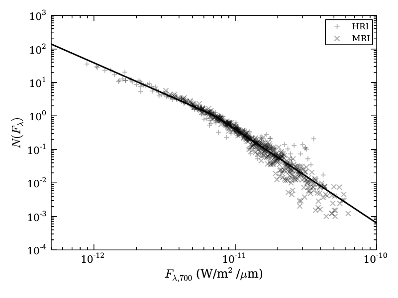
Figure 11: Combined HRIVIS and MRI flux distributions ($F_{\lambda}\geq\mbox{$F_{\lambda,{\rm min}}$}$), scaled to $N(F_{\lambda}=7.2\times 10^{-12})=1$. For the MRI data, only full-frame distributions from $\Delta>900$ km are shown. The solid line is our best-fit broken power-law (Eq. 3).

4.2 Total particle flux

Due to the great numbers of large particles, we can only accurately measure the total scattered flux from the brightest particles in each image. Our best estimate of the fraction of the coma flux attributable to large particles is 0.11% for fluxes ranging $0.9-4.7\times 10^{-11}$ W cm^-2 µm^-1 (row labeled “MRI (distant)” in Table 3). This estimate was derived from images with relatively little point source crowding ($\Delta>2000$ km), and a moderate number of particle measurements ($N>300$ particles). In order to build a complete census of the particles, we need to extrapolate the results from that limited range down to the faint end of the distribution. We find that the brightest particles observed throughout the closest approach images are consistently near $\mbox{$F_{\lambda,700}$}=4.5\times 10^{-11}$ W cm^-2 µm^-1. On the other end, the faintest particles we can manually find and measure have fluxes of order $\mbox{$F_{\lambda,700}$}\sim 10^{-13}$ W cm^-2 µm^-1 (Fig. 12). If the very steep flux distribution we derived in §4.1 extends from $\mbox{$F_{\lambda,700}$}=1\times 10^{-12}$ down to $1\times 10^{-13}$ W cm^-2 µm^-1, there should be several million particles per image. However, at such great pixel densities (1 particle per 17 pixel area) it should be very difficult to find faint isolated particles (the core of the HRIVIS native PSF has an area of 113 pixels). Furthermore, if we let the flux distribution continue down to $1\times 10^{-14}$ W cm^-2 µm^-1, the large particles account for 100% of the coma flux, leaving no room for any fainter particles (millimeter sized and smaller). Therefore, the flux distribution must change or be truncated at fluxes fainter than $\mbox{$F_{\lambda,700}$}=1\times 10^{-12}$ W cm^-2 µm^-1. The uncertainty in the lower flux limit is a major source of error in all estimates of the total number, flux, cross section, and similar derived quantities. We list the results from our extrapolations in Table 4. We estimate that the large particles account for 2–14% of the total coma flux near the nucleus.

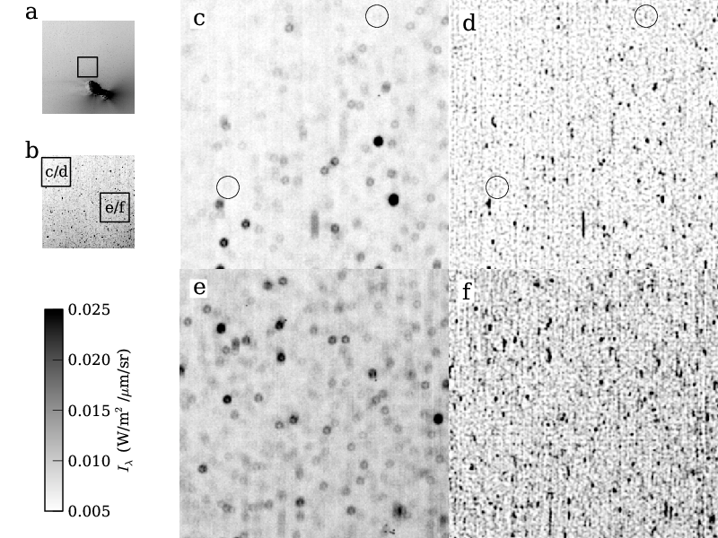
Figure 12: Two sub-frames of HRIVIS image hv5004031 ($\Delta=694$ km) showing the crowded field of particles: a) an MRI context image (mv5004046) with the approximate HRIVIS field of view outlined with a box (image is log scaled from 0.001 to 1.0 W m^-2 µm^-1 sr^-1); b) HRIVIS image, sub-frames c/d and e/f are outlined and labeled; c) HRIVIS sub-frame; d) the same as c, but deconvolved to enhance the spatial resolution; e) another HRIVIS sub-frame; f) panel e, deconvolved. Two particles with fluxes near $1-2\times 10^{-13}$ W m^-2 µm^-1 have been circled. The HRIVIS field of view is 1.4 km, and the sub-frames are 0.42 km.

If we take the the first image in which particles are easily seen, mv5002051 at $\Delta=5148$ km (Fig. 13), we can estimate the total number of particles within a 20.6 km radius (the largest circular aperture centered on the nucleus that fits within the image). We find a total coma flux of $(2.15\pm 0.22)\times 10^{-7}$ W m^-2 µm^-1 (includes the bright jets, but not the nucleus) and assume that 2–14% of that flux is attributable to large particles. The results are presented in Table 4 and will be used below when we estimate the cross section, mass, and water production rate of the large particles.

Up to now, we have not addressed streaked particles in our MRI images. If a significant fraction of the flux in our images at $\Delta\approx 2400$ km is contained within streaked particles then our estimates on the total flux and number of large particles will be systematically low. However, we find that few particles are streaked and the correction to include any possible streaks is negligible. To demonstrate, we developed a Monte Carlo simulation that uses the spacecraft position and velocity to estimate the volume of space that is smeared. Within a 20.6 km projected radius, 2% the field-of-view is smeared over $\geq 1.5$ MRI pixels, and only particles outside of 120 km are smeared this much. If the particle density follows a $r^{-2}$ profile, the fraction of smeared particles reduces to effectively zero.

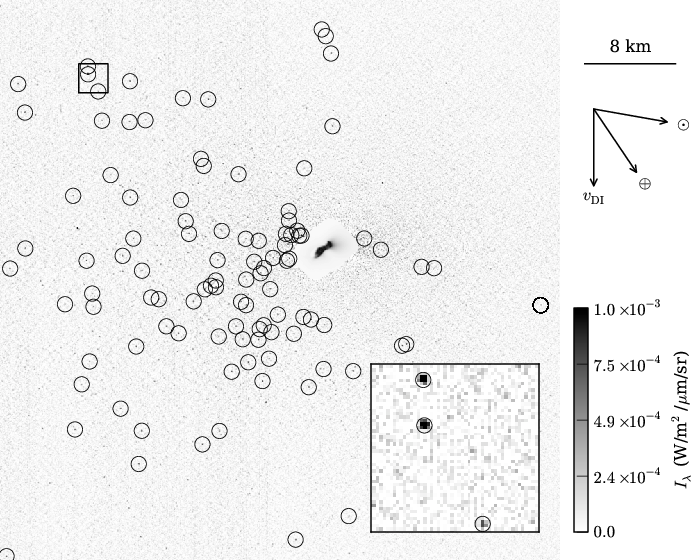
Figure 13: Image mv5002051, background coma removed. Point sources identified by DAOPHOT with fluxes greater larger than the image’s 80% completeness limit are circled to show the extent of the large particle coma (particles below this limit can still be seen by eye). An image of the nucleus has been inserted into the central masked region. The box marks the location of the inset image. Stars, most of which have been automatically masked, are streaked over 13 pixels in this image.

5 Particle size and composition

In the absence of any compositional information on these large particles, we assume two cases to demonstrate their likely range of sizes. First, we will consider that the particles are refractory, and photometrically behave like comet nuclei (the “dusty” case). Then, we will consider that the particles are icy, and behave like the icy satellite Europa (the “icy” case). We stress that these two cases are examples only. They may not reflect the true nature of the particles, but they do yield useful limits on the particle sizes. We will show that the particles are much larger than the 0.1–100 µm sizes typically considered in comet dust. We purposefully avoid interpreting the large particles with phase functions that have been derived for comet comae. Light scattered by comet dust comae is expected to be dominated by dust grains in the sub-micrometer to micrometer size range (Kolokolova et al. 2004), which scatter optical light differently than centimeter-sized particles.

First we take the case in which the particles photometrically behave like comet nuclei, i.e., they have a very low albedo, and have a phase angle behavior like a macroscopic object and not like small dust grains. We refer to this case as the “dusty case,” but, just like comet nuclei, these model particles may be internally icy. We adopt the geometric albedo ($A_{p}=0.049$) and phase function ($-2.5\log{\Phi}=0.046\theta$ mag for $\theta$ in units of degrees) of Hartley 2’s nucleus (Li et al. this issue). The geometric albedo is defined as the ratio of the energy scattered from the object toward a phase angle of 0^∘ to that scattered from a white Lambertian disk with the same cross section (cf. Hanner et al. 1981 for this and other relevant albedo definitions).

In Section 4.1, we found that individual particle fluxes range from $F_{\lambda,700}$$=1\times 10^{-13}$ to $4.5\times 10^{-11}$ W m^-2 µm^-1, where $F_{\lambda,700}$ is the particle flux normalized to a distance of 700 km. To convert between flux and cross section, we use the formula

$$F_{\lambda}=A_{p}\Phi(\theta)\sigma\frac{S_{\lambda,\odot}}{r_{h}^{2}}\frac{1}{\Delta^{2}}$$ (4)

where $F_{\lambda}$ is the particle flux in units of W m^-2 µm^-1, $\sigma$ is the cross-sectional area of the particle (cm²), $S_{\lambda,\odot}$ is the solar flux density at 1 AU (W m^-2 µm^-1), $r_{h}$ is the heliocentric distance of the particle (1.064 AU), and $\Delta$ is the spacecraft-particle distance (cm). For the HRIVIS and MRI CLEAR1 filters, we use a solar flux density of 1471 and 1435 W m^-2 µm^-1, respectively (Klaasen et al. in prep.). To convert from cross section to effective radius, we assume a spherical geometry: $\sigma=\pi a^{2}$. Altogether, assuming a comet nucleus-like photometric behavior, the effective radii of the particles range from 10 to 221 cm. The largest of these particles (4 m diameter) are just over the resolution of the HRIVIS reconstructed frames (about 3 m at a distance of 700 m). We consider these sizes to be an upper limit to the true particle sizes. For a lower-limit estimate, we consider the case where the particle scattering function is similar to the icy satellite Europa: $A_{p}=0.67$ and $\Phi=1.0-0.01\theta+2.2\times 10^{-5}\theta^{2}$ (Buratti and Veverka 1983, Grundy et al. 2007). At a phase angle of 80^∘, Europa’s phase function is 0.34. For this parameter set the effective radii are 0.8 to 17 cm.

Following Eq. 4, where flux is proportional to cross-sectional area, we can compute the total observed particle cross section and add it to Table 4. We have assumed our icy particle case, using the photometric parameters of Europa. To instead use our dusty case, multiply the cross sections in the table by 158.

Our flux distributions imply a very steep size distribution. Assuming a spherical geometry, the differential size distribution is

$$\frac{dn}{da}=2N_{0}F_{1}^{\alpha+1}a^{2\alpha+1},$$ (5)

where $F_{1}$ is the flux from a 1 cm radius particle in units of W m^-2 µm^-1, and particle radius $a$ is in units of cm. The constant $N_{0}$ is the solution to the equation:

$$N=N_{0}\int_{F_{\lambda,{\rm min}}}^{F_{\lambda,{\rm max}}}\frac{dn}{dF}dF,$$ (6)

using the appropriate values from Table 4. Our low-flux power-law slope ($\alpha=-2.85$) corresponds to a size distribution proportional to $a^{-4.7}$. This slope is steeper than the many size distribution estimates of small through large dust grains ($a\sim 1$ µm to 1 mm with slopes near $-4$ to $-3$) based on grain thermal emission (Lisse et al. 1998, Harker et al. 2002, 2011), grain dynamics (Fulle 2004, Reach et al. 2007, Kelley et al. 2008, Vaubaillon and Reach 2010), and dust flux monitors on spacecraft (McDonnell et al. 1987, Green et al. 2004). Specifically for Hartley 2, Bauer et al. (2011) estimate the comet’s overall size distribution to follow a power-law slope of $-4.0\pm 0.3$, derived by comparing $R$-band and WISE 12 and 22 µm fluxes. Epifani et al. (2001) fit an ISOCAM 15 µm image of the comet taken about 10 days after perihelion with a dust dynamical model. They report a time-averaged power-law slope of $-3.2\pm 0.1$, but inspection of their Fig. 10 suggests $-3.8$ is more appropriate (their best-fit slopes never fall above $-3.5$). These slopes are shallower than our value of $-4.7$, but there is no requirement that they be the same.

To better understand the size, and thereby the composition, of the large particles, we investigate the largest particle that may be lifted from the nucleus, $a_{crit}$. This parameter is estimated by comparing the force of gravity to the gas drag force at the surface of the comet. Meech and Svoren̆ (2004) integrated the equation of motion for spherical particles ejected from a spherical nucleus and found

$$a_{crit}=\frac{9\mu\mbox{$m_{\rm H}$}Qv_{th}}{64\pi^{2}\rho_{p}\rho_{N}R_{N}^{3}G},$$ (7)

where $\mu$ is the atomic weight of the gas (amu), $m_{\rm H}$ is the mass of hydrogen (g), $Q$ is the gas production rate (s^-1), $v_{th}$ is the mean thermal expansion speed of the gas (cm s^-1), $\rho_{p}$ is the density of the particle (g cm^-3), $\rho_{N}$ is the density of the nucleus (g cm^-3), $R_{N}$ is the radius of the nucleus (cm), and $G$ is the gravitational constant (cm³ g^-1 s^-2). With the shape model of Comet Hartley 2, Thomas et al. (this issue) estimate the surface gravity of the nucleus to be $a_{N}=0.0019-0.0044$ cm s^-2, which includes the rotation state of the nucleus. Therefore, we re-write the equation from Meech and Svoren̆ (2004) to use the gravitational acceleration at the nucleus

$$a_{crit}=\frac{3\mu\mbox{$m_{\rm H}$}Qv_{th}}{16\pi\rho_{p}a_{N}R_{N}^{2}}.$$ (8)

The bulk material density for dust is $\sim 3$ g cm^-3 and for ice is 1.0 g cm^-3. For the dusty case, we will consider porous aggregates of dust with a total density of 0.3 g cm^-3 (i.e., 90% vacuum). For the icy case, we will at first assume 1.0 g cm^-3, but later consider porous aggregates with $\rho_{p}=0.1$ g cm^-3.

The total water production rate of Comet Hartley 2 near closest approach has been estimated via several methods to be $Q(\mbox{H${}_{2}$O})\approx 0.7-1.2\times 10^{28}$ s^-1 (A’Hearn et al. 2011, Combi et al. 2011, Dello Russo et al. 2011, Meech et al. 2011, Mumma et al. 2011, Knight and Schleicher this issue). Yet, the coma contains a significant amount of water ice (A’Hearn et al. 2011, Protopapa et al. 2011), which could be supplying a large fraction of the water vapor around the comet. Moreover, the water production rate is not uniformly distributed over the surface (A’Hearn et al. 2011). We can account for these observations by multiplying the water production rate by the ratio $f_{surface}/f_{active}$, where $f_{surface}$ is the fraction of the water vapor produced at the surface of the nucleus, and $f_{active}$ is the areal fraction of surface that is active. For illustrative purposes, we will assume that 1% of the water vapor is produced from 10% of the surface. The remaining 99% of the water vapor sublimates from the icy grain halo.

For a nucleus water production rate of $Q(\mbox{H${}_{2}$O})f_{surface}/f_{active}=10^{27}$ s^-1, $v_{th}=0.5$ km s^-1, Hartley 2’s mean radius (0.58 km), mean surface gravity, and assuming a particle density of pure ice ($\rho_{p}=1$ g cm^-3), we find $a_{crit}=8$ cm. If we instead take CO₂ as the driving gas, with a production rate of $10^{27}$ s^-1 (A’Hearn et al. 2011), $f_{surface}=100\%$, and $f_{active}=10\%$, then $a_{crit}$ becomes 200 cm for solid ice spheres. Based on this exercise, the icy model size estimates, $a\leq 17$ cm, are reasonable.

If instead of icy particles, we assume nucleus-like particles with a density of 0.3 g cm^-3, our $a_{crit}$ estimates increase to 28 cm (H₂O) and 670 cm (CO₂). Compared to our size estimates of $a\leq 210$ cm, dark, dusty particles are plausible if CO₂ is the driving gas; water can be made consistent if $f_{surface}/f_{active}$ is increased to 1.0.

Aggregate particles are more easily lifted by gas drag due to their larger surface area per mass. Nakamura and Hidaka (1998) found that the drag force for an aggregate is approximately the same as the drag force on an area-equivalent sphere (with an error of less than 40% in the large aggregate limit). Since our particle radii are based on the observed flux, which is proportional to the cross-sectional area, our radii are already defined by area-equivalent spheres. Therefore, by revising our particle density we can use Eq. 8 to estimate $a_{crit}$ for aggregates.

We assembled model particles using a ballistic particle-cluster aggregate (BPCA) method (Meakin 1984). As the size of the aggregate grows beyond a few thousand monomers the density asymptotically approaches 10% of the bulk material density. Thus, for a refractory material with a bulk density near 3 g cm^-3, a centimeter-sized BPCA particle would have a density of 0.3 g cm^-3. The $a_{crit}$ estimates will be the same as in our nucleus-like case above.

Treating the large particles as aggregates rather than solid spheres better agrees with the HRIIR spectra of the coma. A’Hearn et al. (2011) and Protopapa et al. (2011) studied the water ice absorption features and found that they are most consistent with icy aggregates with monomer radii $\approx 1$ µm. An icy BPCA particle would have a density of 0.1 g cm^-3. The lowered density for icy aggregates increases $a_{crit}$ by a factor of 10, giving us a healthy margin for launching large icy particles off the surface of the nucleus, even where water sublimation is driving the activity.

In summary, the dusty particle case produces very large particle estimates (up to 2 m in radius) that are just at the resolution limit of the HRIVIS instrument. Gas expansion from CO₂ is sufficient to lift these large particles from the surface of the comet if they have a comet-like density of $\approx 0.3$ g cm^-3. The water-ice case produces particle estimates up to $\approx 20$ cm in radius, which are easily lifted from the nucleus by water or CO₂ expansion.

6 Spatial distribution and origin

Mapping the spatial distribution of the particles gives clues to their origins and dynamics. In Figs. 14–17, we plot the column density of particles and total coma surface brightness contours for all 501 and 121 ms MRI images listed in Table LABEL:tab:fits. The column density images were derived from our final photometry lists for $F_{\lambda}>F_{\lambda,{\rm min}}$, binned onto a $38\times 38$ pixel grid. Inspection of the figures reveals that the coma and the particles have different spatial distributions. The particles are biased to the anti-sunward direction on scales $>2-4$ km, whereas the coma distribution is dominated by the jets. This asymmetry is especially apparent in the strong sunward jets, where the particle density is lower than in other regions of similar surface brightness. It is not an observational bias; we have masked those regions close to the nucleus where the column density and jet morphology interfere with the PSF fitting process. Instead, the low particle density in the sunward jets can be accounted for by particle dynamics. We consider three dynamical processes that could be affecting the particle distribution: (1) the rotation of the nucleus; (2) solar radiation pressure; and (3) a rocket effect from sublimating ice. Hydrodynamic flows from the strong gas production rates and asymmetry in outgassing may also play a role in the particle dynamics, but this analysis is outside the scope of this paper.

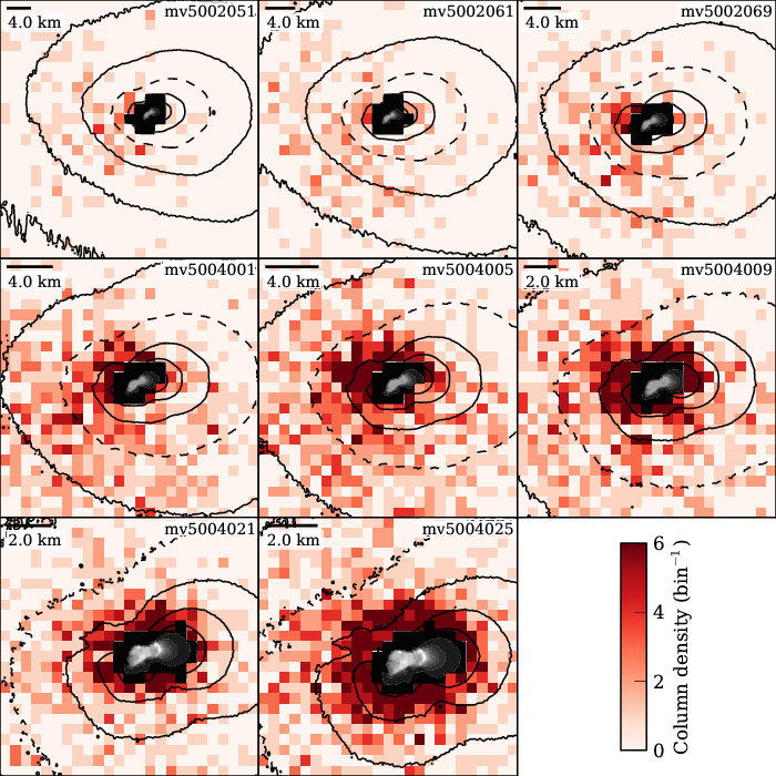
Figure 14: Contours of the total coma surface brightness superimposed over particle column density for 501 and 121 ms MRI images mv5002051 through mv5004025. The contours are spaced at factor of 2 intervals, and the dashed line is 0.008 W m^-2 µm^-1 sr^-1. The coma image was smoothed with a Gaussian kernel function (7 pixel FWHM) before the contours were created. Only particles with $F_{\lambda}>F_{\lambda,{\rm min}}$ are considered, and the particle bins are $38\times 38$ pixels in size. The region closest to the nucleus is masked from the analysis, and has been replaced with each epoch’s image of the nucleus and inner-most coma. In all images, the projected velocity of the spacecraft is toward the bottom, and the sunward direction is approximately to the right.

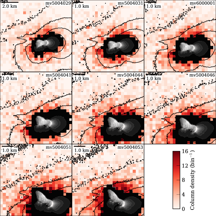
Figure 15: Same as Fig. 14, but for images mv5004029 through mv5004053.

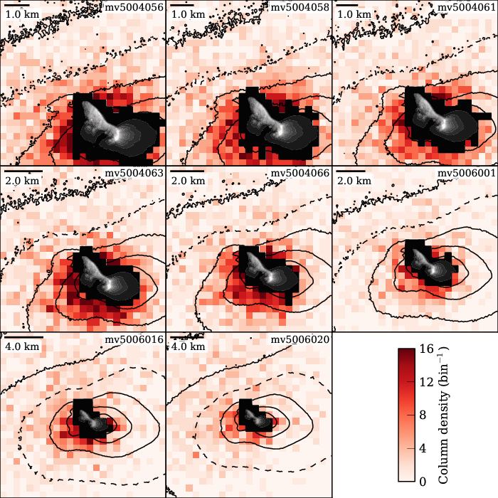
Figure 16: Same as Fig. 14, but for images mv5004056 through mv5006020.

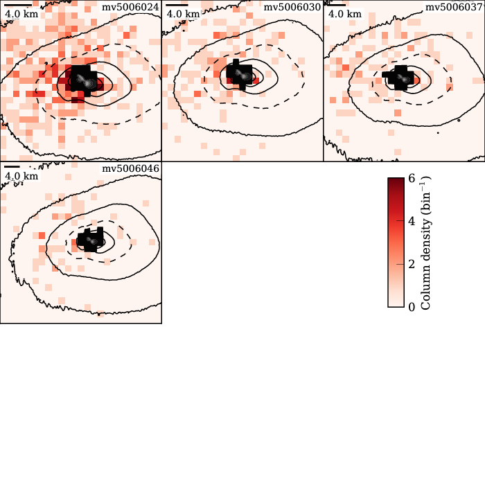
Figure 17: Same as Fig. 14, but for images mv5006024 through mv5006046.

6.1 Radial expansion and nucleus rotation state

Rotation of the nucleus has a direct impact on the spatial distribution of particles. To estimate this effect, we must first recognize that the particle outflow speeds are low. In order for the particles to be seen as point sources in HRIVIS images at closest approach, their speeds must be lower than $\approx 3~{}\mbox{m}/0.376~{}\mbox{s}=8$ m s^-1. A lower constraint is computed by Hermalyn et al. (this issue) based on the 3D positions of the particles. They find 0.5–2 m s^-1 to be more typical (note that these speeds are not necessarily radial). At such low speeds, the large particles take $\gtrsim 10^{3}$ s to reach 2 km from the nucleus. In contrast, small dust grains move much more quickly with outflow speeds expected to be of order 100 m s^-1. The fine dust reaches 2 km in as little as 20 s.

The positions of the major jets are governed by the rotation of the long axis about the angular momentum vector, with a period of 18.4 h near closest approach; the long axis is inclined to the angular momentum vector by 81^∘ (Belton et al. this issue). Taking 1 m s^-1 as the particle outflow speed from the surface, the nucleus will have rotated 10^∘ by the time the particles have traveled 2 km. So, the rotation state has a minor consequence on the distribution of particles at 2 km, and their spatial distribution should be closely related to their source regions. This observation and the assumption of radial motion suggests that the strong sunward jets are not the primary source of the large particles, but instead they are ejected from along the long-axis of the nucleus. The jets pointed towards the bottom of the images in Fig. 15 would be the next likely source region for particles. There is also a large population of particles towards the top of Figs. 14 and 15, but they do not have an apparent source region (i.e., this side of the nucleus does not appear to be as active as the other regions). However, we note that not all potential sources are apparent in the MRI images. For example, the apparent water jet seen in Fig. 5 of A’Hearn et al. (2011), which points to the top right of Figs. 16 and 17, has no clear optical counterpart but may also contribute to the large particle production (n.b., this water jet does not appear to contain ice, and therefore is unlikely to be a source of large icy particles).

Taking a lower ejection speed of 1 cm s^-1, the nucleus can rotate three times before particles travel 2 km. Thus on this length scale, and in the absence of any other perturbing forces, the particles would have a spatial distribution correlated with the activity profile of the nucleus. Because the CO₂ and H₂O gas production rates and the optical light curve peak when the small end is pointed towards the Sun (A’Hearn et al. 2011), in the absence of other forces the large particle density should peak in the solar direction, which is not observed.

6.2 Solar radiation pressure

In principle, solar radiation pressure could redistribute large particles into the anti-sunward direction. The acceleration from radiation, $a_{rad}$, in units of cm s^-2 is (Burns et al. 1979)

$$a_{rad}=\frac{Q_{pr}S_{\odot}\sigma}{cmr_{h}^{2}},$$ (9)

where $Q_{pr}$ is the radiation pressure efficiency factor, $S_{\odot}$ is the integrated flux density ($1.361\times 10^{6}$ erg cm^-2 s^-1 at 1 AU), $\sigma$ is the geometrical cross section of the particle (cm²), $c$ is the speed of light (cm s^-1), $m$ is the mass of the particle in question, and $r_{h}$ is the heliocentric distance (AU). We have already dropped all velocity dependent terms from $a_{rad}$ (cf. Burns et al. 1979). It is common to express radiation pressure with the parameter $\beta$ defined as the ratio of the force of solar radiation pressure to the gravitational force from the Sun,

$$\beta\equiv\frac{F_{rad}}{F_{grav}}=\frac{5.7\times 10^{-5}Q_{pr}}{\rho_{p}a}.$$ (10)

The radiation pressure efficiency is 1 for perfectly absorbing, isotropically emitting spheres. For our particles, we again take the icy particle case and derive $Q_{pr}$ from the phase function and geometric albedo (van de Hulst 1957): $Q_{pr}\approx 1-A_{B}\overline{\cos{\alpha}}$, where $A_{B}$ is the Bond albedo, and $\overline{\cos{\alpha}}$ describes the anisotropy of the scattered light, where $\alpha=180-\theta$ is the scattering angle. The relationship between the Bond albedo and geometric albedo is $A_{B}=A_{p}\int_{0}^{\pi}\Phi(\alpha)\sin{\alpha}d\alpha$ (Hanner et al. 1981). Altogether, we compute $Q_{pr}=1.58$. For the mass, we again assume two cases for particles with $a=10$ cm: (1) solid spheres with the density of ice, 1 g cm^-3; and (2) compact aggregates of ice (1 µm radius monomers) with an overall particle density of 0.1 g cm^-3. For the latter case, we note that detailed calculations will be required to understand how albedo and the anisotropy of scattering are affected by the complex aggregate shape, and we reserve this investigation for future work. We compute accelerations of $4.8\times 10^{-6}$ and $0.5\times 10^{-6}$ cm s^-2 for 10 cm solid and BPCA aggregate ice particles, equivalent to $\beta=9\times 10^{-6}$, and $1\times 10^{-6}$. For comparison, comet dust trails are comprised of grains with $\beta\lesssim 10^{-3}$ (Sykes and Walker 1992, Reach et al. 2007).

In Figs. 14–17, particles are found out to the image edges in the sunward direction. However, the sunward/anti-sunward asymmetry is clear on 2–4 km length scales. In the rest frame of the comet, the relationship between turnaround distance ($d$), ejection speed ($v_{ej}$), and acceleration from radiation pressure is $d=v_{ej}^{2}/2/a_{rad}$. Solving for ejection speed $v_{ej}$ yields

$$v_{ej}^{2}=\frac{3dQ_{pr}S_{\odot}}{2cr_{h}^{2}\rho_{p}a}=6.0\times 10^{-5}\frac{dQ_{pr}}{\rho_{p}a},$$ (11)

for $v_{ej}$ in units of cm s^-1, $d$ in cm, $\rho_{p}$ in g cm^-3, and $a$ in cm. For our icy particle case $v_{ej}=4.3-6.1(\rho a)^{-1/2}$ cm s^-1 (4–6 cm s^-1 for a 10 cm aggregate, and 1–2 cm s^-1 for solid ice). If particles are truly ejected at these speeds, solar radiation pressure would take $\gtrsim 10^{6}\rho a$ s to accelerate the particles to the $\gtrsim 50$ cm s^-1 speeds measured by Hermalyn et al. (this issue). This result also implies that the dominant velocity component for particles more than a few kilometers from the nucleus would be distinctly in the anti-solar direction, yet only a weak asymmetry in the velocity is observed (Hermalyn et al. this issue). Therefore, radiation pressure does not govern the dynamics for our icy particle cases. The same conclusion is reached for the dusty particle case with a nucleus-like density ($Q_{pr}=1.00$, $\rho_{p}=0.3$ g cm^-3): $v_{ej}=6.3-8.9a^{-1/2}$ cm s^-1 or 0.6–0.9 cm s^-1 for a 100 cm particle.

If we instead assume an ejection speed of 1 m s^-1 for a 10 cm particle, their densities must be $\rho_{p}=2-4\times 10^{-4}$ g cm^-3 in order to be turned around by $d=2-4$ km. Thus, if the particles are very fluffy aggregates, they may be ejected at larger speeds, and radiation pressure will be able to redistribute them into the anti-solar direction, but they could still have instantaneous velocities distributed about the anti-solar vector.

6.3 Rocket effect

The rocket effect is the acceleration of the particles due to the sublimation of water ice. For a spherical geometry with radial outflow,

$$a_{rocket}=\frac{3\mu\mbox{$m_{\rm H}$}Zv_{th}f_{ice}}{4\rho_{p}a}=1.1\times 10^{-18}\frac{Z}{\rho_{p}a},$$ (12)

where $Z$ is the sublimation rate of the particle (molec cm^-2 s^-1), $\mu$ is the molecular weight of the sublimating ice (18 u for water), $m_{\rm H}$ is the mass of hydrogen (g), and $f_{ice}$ is the ice fraction of the particle (all remaining parameters are in cgs units). Following Reach et al. (2009), we define the dimensionless rocket effect parameter $\alpha$ as the ratio of the force from the sublimation mass-loss, $F_{rocket}$, to the force of gravity from the Sun, $F_{grav}$:

$$\alpha\equiv\frac{F_{rocket}}{F_{grav}}=2.238\times 10^{26}\frac{3\mu\mbox{$m_{\rm H}$}Zv_{th}f_{ice}}{4GM_{\odot}\rho_{p}a},$$ (13)

where $G$ is the gravitational constant (cm³ g^-1 s^-2), and $M_{\odot}$ is the mass of the Sun (g). The rocket effect parameter should have a heliocentric distance dependency, since the product $Zv_{th}$ does not necessarily vary as $r_{h}^{-2}$, but Eq. 13 will serve as a good approximation for small $\Delta r_{h}$. The $\alpha$ parameter is analogous to the $\beta$ parameter for dust; both parameters quantify a force directed away from the Sun in fractions of the solar gravitational force.

Assuming no losses from scattering or thermal emission, the maximum water sublimation rate from ice ($Z_{max}$) can be computed from the solar flux density, particle absorption efficiency ($Q_{abs}$), and the latent heat of sublimation for water ice ($L$),

$$Z_{max}=\frac{S_{\odot}Q_{abs}N_{A}}{r_{h}^{2}L}$$ (14)

where $N_{A}$ is Avogadro’s number, and $L$ ranges from $5.0\times 10^{11}$ to $5.1\times 10^{11}$ erg mol^-1 for temperatures from 100 to 300 K (Murphy and Koop 2005). For large compact aggregates (i.e., porous spheres) and solid particles $Q_{abs}\approx 1$, but it is larger for fluffy aggregates since they have light scattering properties more like a collection of monomers, rather than a single solid particle (Kolokolova et al. 2007). This last comment aside, $Z_{max}$ becomes $1.4\times 10^{18}$ molec cm^-2 s^-1 for $T=300$ K. To account for scattering, $Z_{max}$ will scale with $1-A_{B}$, where $A_{B}$ is the Bond albedo. In §6.2 we computed $A_{B}=0.84$ for our icy particle model. Scattering reduces the $Z_{max}$ of the icy model to $Z_{max,icy}=2.2\times 10^{17}$ molec cm^-2 s^-1. For our dusty model, $A_{B}=0.013$ and $Z_{max,dusty}\approx Z_{max}$.

For comparison, consider the model of Beer et al. (2006) for the sublimation rate of icy particles. They employ spherical grains, heated by absorption of sunlight and cooled by thermal emission and sublimation, and computed the absorption and emission efficiencies with Mie scattering and effective medium theory considering both pure ice grains, and “dirty-ice” grains, i.e., ice mixed with a generic absorber (dust). Mixing dust with the ice has a significant effect on the ice equilibrium temperature, but the effect is not a strong function of the ice-to-dust mass ratio (they tested $m_{ice}/m_{dust}=0.9$ and 0.5). Dust should also affect the overall albedo of the particles, but they do not report this parameter. In their Figs. 8 and 9 they present computed grain lifetimes, defined as the time a grain takes to completely sublimate. Their lifetimes for $r_{h}=1.09$ AU are the best examples for our scenario. For $a>0.01$ cm, pure ice grains have lifetimes of $\tau_{pure}=1\times 10^{10}a$ s for particle radius $a$ measured in cm. Dirty-ice grains have a much shorter lifetime: $\tau_{dirty}=1\times 10^{5}a$ s. Since the large particles spend most of their lifetime larger than 0.01 cm, we can transform their lifetimes into sublimation rates:

$$Z=\frac{4\rho_{p}a}{3\mu\mbox{$m_{\rm H}$}\tau f_{ice}}.$$ (15)

The Beer et al. (2006) model sublimation rates for large particles are $Z_{dirty}=4\times 10^{17}$ molec cm^-2 s^-1, and $Z_{pure}=4\times 10^{12}$ molec cm^-2 s^-1. These values are comparable to or less than our maximum sublimation rates.

Taking $Z_{max,icy}$, a 10 cm radius particle is accelerated at a rate $a_{rocket}=0.024$ cm s^-2 away from the Sun, yielding a rocket parameter $\alpha=0.042$, i.e., the rocket effect is 4% the force of solar gravity. For $Z=Z_{max}$, we compute $\alpha=0.27$. Unlike radiation pressure, the rocket effect is potentially very strong.

Acceleration from sublimation will distribute the particles in the anti-solar direction. Following our method for radiation pressure, we can constrain the particle ejection speed with the implied sublimation rate

$$v_{ej}^{2}=2.2\times 10^{-18}\frac{Zd}{\rho_{p}a}.$$ (16)

Again, adopting 2–4 km as our typical turnaround distance, and taking $Z=Z_{max,icy}$, we find ejection speeds of $310-440a^{-1/2}$ cm s^-1 for our solid ice case ($990-1400a^{-1/2}$ cm s^-1 for icy aggregates). These ejection speeds are higher than the instantaneous speeds measured by Hermalyn et al. (this issue), but the two speeds do not need to agree since one is at/near the surface and the other is out in the coma. For $Z=Z_{max}$, the resulting ejection speeds are increased: $v_{ej}=780-1100a^{-1/2}$ cm s^-1 (solid ice) and $2500-3500a^{-1/2}$ cm s^-1 (icy aggregates). However, in the above analysis we have assumed that only the sunlit hemisphere is sublimating. By distributing the sublimation across more of the surface, we can decrease the implied ejection speeds to 10–100 cm s^-1, similar to the speed measured in the coma by Hermalyn et al. (this issue). Therefore, we conclude that a sublimation rate excess on the sunlit hemisphere of order $10^{17}$ molec cm^-2 s^-1 readily describes the sunward/anti-sunward particle asymmetry. Detailed simulations will be needed to fully account for the observed distribution of particle velocities.

7 Mass and water production rate

Table 4 includes the total particle mass, based on our icy photometric model and a particle density of 1 g cm^-3. For the dusty model and $\rho_{p}=0.3$ g cm^-3, the masses are increased by a factor of 672. With our preferred flux lower limit of 0.1–$1.0\times 10^{-12}$, the particle masses correspond to $0.03-0.10M_{N}$ (icy), $23-70M_{N}$ (dusty), where $M_{N}=2.4\times 10^{11}$ g is the mass of the nucleus, assuming a 0.3 g cm^-3 density (Thomas et al. this issue). It is clear that the dusty case is impossible. The only way we can reduce the estimated total mass for these dark particles is by decreasing their densities to well below $10^{-3}$ g cm^-3. Therefore, we do not favor the dusty case, but it does remain as a possible interpretation. Given that the total mass lost from the comet per orbit is of order 1% of the nucleus (Thomas et al. this issue), even the solid ice particles may be too massive. Porous ice particles (e.g., $\rho_{p}=0.1$ g cm^-3) should be considered the most likely case.

Icy particles will begin sublimating as soon as they are released from the nucleus and warmed by insolation. In §6.3, we computed the rocket effect on the particles due to water ice sublimation and concluded that a sublimation rate excess of $10^{17}$ molec cm^-2 s^-1 on the particle’s sunlit hemisphere can describe the observed sunward/anti-sunward asymmetry in particle column density. We also computed the maximum sublimation rate, based on energy balance between absorbed solar radiation and sublimation. We apply this latter value, $Z_{max,icy}$ to all of the large particles and compute water production rates. The total large particle water production rate within a 20.6 km radius aperture is limited to $<0.6-5\times 10^{25}$ molec s^-1, which is $<0.1-0.5$% of the total water production rate of the comet ($\approx 1\times 10^{28}$ molec s^-1). We can change the water production rate by assuming a different photometric model as $Q\propto(1-A_{B})(A_{p}\Phi)^{-1}$. For our nucleus-like case, we find $Q({\rm H_{2}O})<16-80\%$ of the total water production rate, but, unless the particles are fluffy aggregates with $\rho\lesssim 10^{-3}$ g cm^-3, we rule out this case based on their mass. The icy particle case yields our best estimate of the water production rate, $Q({\rm H_{2}O})<(1-5\times 10^{-3})Q_{total}$.

8 Comparison to other observations

Harmon et al. (2011) observed comet Hartley 2 with Arecibo S-band ($\lambda=12.6$ cm) radar at the end of October 2010, about a week before Deep Impact’s closest-approach. In their average Doppler spectrum, they observe a strong grain-coma echo, with a characteristic radial velocity dispersion of 4 m s^-1. The velocity distribution is asymmetric, with a range of $\approx-50$ to $+13$ m s^-1 with respect to the nucleus (negative velocities are away from the Earth). The coma has a strongly depolarized echo, which indicates the radii of the largest particles are well above the Rayleigh limit of $\lambda/2\pi=2$ cm. Harmon et al. (2011) suggest that there exists a significant population of particles with decimeter sizes or larger. We explore the possibility that the radar observations may be the large particles imaged by Deep Impact.

The average radar cross section of the coma was 0.89 km². From our MRI observations, we derived a total icy particle cross section of $\sigma=4\times 10^{-4}$ to $3\times 10^{-3}$ km² within 20.6 km from the nucleus. Our cross section is more than two orders of magnitude smaller than the radar observed cross section. However, their beam is much larger than what the MRI can image when individual particles are detectable. We have found particles out to 40 km in Fig. 13, but the Arecibo beam size is 32,000 km at the distance of the comet. With speeds of order 4 m s^-1, and lifetimes of order $10^{5}$ s (dirty ice), the large icy particle coma would extend out to $\sim 400$ km. This estimate implies our census of the large particles is incomplete by about a factor of $<400/20.9=20$, resulting in a total icy particle cross section of $\lesssim 0.01$ km², which still remains inconsistent with the radar results.

Assuming for the moment that the radar cross section properly reflects the total icy particle population we compute an upper limit to the total water production rate of $<2\times 10^{27}$ molec s^-1. The SWAN instrument on the SOHO satellite observes Ly$\alpha$ emission over fields of view much larger than the radar beam size ($10^{5}$ km pixel^-1). These observations are a good point of reference for a total water production rate that is sure to include water produced by any large particles observed with Arecibo. Combi et al. (2011) measured a water production rate of 6–$9\times 10^{27}$ molec s^-1 near perihelion (Combi et al. 2011). By this estimate, it seems that the large particles could account for a substantial fraction of the total water production rate of the comet. Note, however, that the SWAN-based water production rates are on par with those observed in 4000 km apertures and smaller. Based on the aperture sizes and water production rates listed in Table 5, most of the water is produced close to the nucleus, perhaps within a few tens or hundreds of kilometers, suggesting that the Arecibo observed particles have a low water sublimation rate, if any.

A dusty large particle population yields a cross section of $\sigma=0.07-0.5$ km² (§5), which is in better agreement with the radar results, but suggests that the entire large particle coma is within $\sim 40--250$ km from the comet. There is no indication in Figs. 14 and 17 that the large particle coma is truncated on this length scale. Moreover, dusty particles may not have sublimating ice. Instead, they could fragment into finer particles. If the large particles are dusty, they must fragment on $\lesssim 40--250$ km length scales in order to keep their total cross section less than or equal to the observed radar cross section. Just based on the observed cross sections, we consider the dusty case to be less likely than the icy case, but still find the icy case to be lacking. Of course, a coma of both icy and dusty particles is possible. More information on the composition and light scattering properties, including radar wavelengths, will be needed to reconcile the radar and MRI observations.

9 Summary

Comet Hartley 2 is surrounded by a coma of large particles with radii $\gtrsim 1$ cm. With observations from Deep Impact, we measured their total flux and flux distribution, based on photometry of individual particles. The flux distribution of these particles implies a very steep size distribution with power-law slopes ranging from $-6.6$ to $-4.7$. We estimate that the particles account for 2–14% of the total flux from the near-nucleus coma. The spatial distribution of the particles is biased to the anti-sunward direction, as observed by the spacecraft both pre- and post-closest approach. Radial expansion from the active areas of the rotating nucleus does not explain the observed spatial distribution, even if the ejection speeds are very low ($\sim 1$ cm s^-1). Radiation pressure from sunlight cannot redistribute them into the anti-sunward direction on small enough length scales unless the particles have extremely low densities ($\sim 10^{-4}$ g cm^-3) or low radial ejection velocities ($\lesssim 10$ cm s^-1). Low ejection velocities suggest there should be a strong anti-sunward velocity component in the coma, but this does not agree with the velocity distribution observed by Hermalyn et al. (this issue).

We examined two possible particle compositions. Our models were based on the photometric properties of the nucleus of Hartley 2 (dusty case: low albedo, 0.3 g cm^-3) and the Jovian satellite Europa (icy case: high albedo, 0.1–1.0 g cm^-3), and serve as approximate limiting cases.

The dusty case produces particle size estimates ranging from 10 cm to 2 m in radius, the largest of which is just at the limiting resolution of Deep Impact’s HRIVIS camera at closest approach. Such large particles may be lifted off the nucleus by gas drag if CO₂ is the driving gas. Water is a plausible alternative if the water production rate from the nucleus is at least $10^{27}$ molec s^-1. Based on the dusty model, the total large particle cross section within 20.6 km from the nucleus is 0.07-0.5 km², similar to the 0.89 km² radar cross section observed by Harmon et al. (2011). If these particles are mini-nuclei, we estimate they account for 16–80% of the comet’s total water production rate (within 20.6 km). However, we can all but rule out the dusty case based on total mass estimates of the large particles, which are in excess of 10 nucleus masses for densities of 0.3 g cm^-3. Densities $\lesssim 10^{-3}$ g cm^-3 are required to reduce the total mass of the particles to a few percent of the nucleus, which is needed to keep the particle mass less than the total mass lost from the comet per orbit (2% during the 2010 apparition; Thomas et al. this issue).

The icy case produces particle size estimates ranging from 1 to 20 cm in radius. These particles are easily lifted by water and CO₂ gas drag. Icy particles would sublimate as soon as they are heated by sunlight. If the particles have a net sublimation on their sunlit sides, they would feel a rocket force that could easily distribute the particles into the anti-sunward direction. The sublimation rate excess required for this redistribution is $\lesssim 10^{17}$ molec cm^-2 s^-1, where the exact value depends on the particle ejection velocities. The cross section of icy particles within 20.6 km is much smaller than the observed radar cross section by two to three orders of magnitude. The water production rate of the Deep Impact observed particles is limited to $<0.1-0.5$% of the comet’s total water production rate. The total mass of the particles for a density of 1 g cm^-3 is 3–10% the total mass of the nucleus. Thus, porous aggregates with $\rho_{p}\lesssim 0.1$ g cm^-3 should be considered more likely than solid ice particles.

We consider the icy case to be more likely than the dusty case for three reasons: (1) the icy particles are more easily lifted by gas drag; (2) we can account for the sunward/anti-sunward asymmetry in the particle distribution if ice is sublimating on their sunlit sides; and (3) the total large particle mass for the dusty case is much greater than the total mass of the nucleus. However, several details are needed in order to test our hypothesis. We need an improved icy particle model that treats the large particles more like macroscopic objects to better understand their water production rates (if icy) and light scattering properties (dusty or icy). We need to better constrain the particle densities, which may rule out the dusty case. A hydrodynamic analysis of the near-nucleus coma, especially around the highly active small end, would improve our knowledge of the dynamics of large particles. A better understanding of the radar coma that includes grains smaller than $\lambda/2\pi$ could help resolve the discrepancy between our icy particle cross section and the observed radar coma cross section.

If indeed icy with a high albedo, the large particles do not appear to be the source of the comet’s enhanced water production rate; although, as discussed above, there is much work that can be done to refine this conclusion. We suspect that the small icy grains in the jets, as observed in Deep Impact IR spectra (A’Hearn et al. 2011, Protopapa et al. 2011), are a significant source of water, and the primary cause of the hyperactivity of Comet Hartley 2.

Table 1: HRIVIS and MRI images considered in this paper. Table columns are: $t-t_{enc}$, time relative to encounter; Exp., exposure time; $\Delta$, spacecraft-comet distance; Scale, pixel scale at the distance of the comet; $\phi$, phase (Sun-comet-spacecraft) angle.

Image	$t-t_{enc}$	Exp.	$\Delta$	Scale	$\phi$
	(s)	(ms)	(km)	(m)	(∘)
HRIVIS
hv5004024	$-$48.4	375.5	915	1.8	79.6
hv5004025	$-$39.4	125.5	847	1.7	79.3
hv5004027	$-$29.1	375.5	781	1.6	79.0
hv5004028	$-$18.8	125.5	732	1.5	79.0
hv5004030	$-$9.8	375.5	704	1.4	79.1
hv5004031	$-$0.7	125.5	694	1.4	79.6
hv5004033	9.6	375.5	704	1.4	80.5
hv5004034	19.8	125.5	735	1.5	81.5
hv5004036	30.2	375.5	787	1.6	82.7
hv5004037	40.1	125.5	851	1.7	83.8
MRI
mv5002051	$-$414.0	500.5	5148	51.5	84.8
mv5002061	$-$326.5	500.5	4082	40.8	84.4
mv5002069	$-$254.4	500.5	3210	32.1	84.0
mv5004001	$-$196.8	500.5	2523	25.2	83.4
mv5004005	$-$167.0	500.5	2172	21.7	83.0
mv5004009	$-$139.8	500.5	1858	18.6	82.6
mv5004012	$-$119.9	40.5	1632	16.3	82.1
mv5004014	$-$109.1	120.5	1513	15.1	81.8
mv6000000	$-$100.3	40.5	1418	14.2	81.6
mv5004021	$-$89.5	120.5	1303	13.0	81.2
mv5004023	$-$79.6	40.5	1202	12.0	80.9
mv5004025	$-$69.9	120.5	1107	11.1	80.5
mv5004027	$-$59.0	40.5	1006	10.1	80.1
mv5004029	$-$54.2	120.5	964	9.6	79.9
mv5004030	$-$49.2	40.5	922	9.2	79.7
mv5004031	$-$44.5	120.5	885	8.8	79.5
mv5004032	$-$39.5	40.5	848	8.5	79.3
mv6000001	$-$34.7	120.5	815	8.2	79.2
mv5004040	$-$29.9	40.5	786	7.9	79.0
mv5004041	$-$25.0	120.5	760	7.6	79.0
mv5004042	$-$20.0	40.5	737	7.4	79.0
mv5004044	$-$15.3	120.5	719	7.2	79.0
mv5004045	$-$10.3	40.5	706	7.1	79.1
mv5004046	$-$5.5	120.5	697	7.0	79.3
mv6000002	$-$0.6	40.5	694	6.9	79.6
mv5004051	4.2	120.5	696	7.0	80.0
mv5004052	9.1	40.5	703	7.0	80.4
mv5004053	14.0	120.5	715	7.2	80.9
mv5004054	18.9	40.5	732	7.3	81.4
mv5004056	23.7	120.5	753	7.5	82.0
mv5004057	28.6	40.5	778	7.8	82.6
mv5004058	33.5	120.5	807	8.1	83.1
mv6000003	38.5	40.5	840	8.4	83.7
mv5004061	44.2	120.5	882	8.8	84.3
mv5004062	49.1	40.5	921	9.2	84.8
mv5004063	54.1	120.5	962	9.6	85.2
mv5004064	59.0	40.5	1004	10.0	85.7
mv5004066	68.9	120.5	1096	11.0	86.5
mv5006000	78.8	40.5	1192	11.9	87.2
mv5006001	88.7	120.5	1294	12.9	87.7
mv6000004	98.7	40.5	1399	14.0	88.2
mv5006011	109.5	120.5	1517	15.2	88.7
mv5006012	119.5	40.5	1627	16.3	89.1
mv5006016	142.4	500.5	1886	18.9	89.8
mv5006020	171.1	500.5	2219	22.2	90.4
mv5006024	207.1	500.5	2643	26.4	91.0
mv5006030	265.7	500.5	3345	33.5	91.6
mv5006037	335.2	500.5	4187	41.9	92.1
mv5006046	403.9	500.5	5023	50.2	92.4

Table 2: Online only table. All single power-law flux distributions derived from HRIVIS and MRI images. Table columns: $F_{\lambda}$, the minimum, maximum, and total particle fluxes in the fit; $N$, number of particles in the fit; $\alpha$, best-fit power-law slope and uncertainty; $P_{KS}$, the Kolmogorov-Smirnov probability that the distribution is a power-law; $F_{T}/F_{coma}$, the fraction of the total coma flux attributable to point sources with $F_{\lambda}>F_{\lambda,{\rm min}}$ in MRI full-frame data, excluding regions near the nucleus.

Image	$\Delta$	$F_{\lambda}$ ${}^{\mbox{a}}$				$N$	$\alpha$		$P_{KS}$	$F_{T}/F_{coma}$
		min	max	total
	(km)	($10^{-12}$ W m-2 µm-1)							(%)
HRIVIS
hv5004024	915	1.8	20.5	1853		641	-3.06$\,\pm\,$	0.09	0.3	$\cdots$
hv5004025	847	1.5	31.6	3128		986	-2.88$\,\pm\,$	0.06	$<$0.1	$\cdots$
hv5004027	781	1.4	29.0	1388		430	-2.86$\,\pm\,$	0.08	0.6	$\cdots$
hv5004028	732	1.5	33.1	2058		685	-2.91$\,\pm\,$	0.07	12.9	$\cdots$
hv5004030	704	0.9	35.5	1222		613	-2.67$\,\pm\,$	0.07	16.8	$\cdots$
hv5004031	694	1.5	40.6	1252		419	-2.70$\,\pm\,$	0.09	13.4	$\cdots$
hv5004033	704	0.9	34.3	918		379	-2.67$\,\pm\,$	0.08	15.2	$\cdots$
hv5004034	735	1.5	31.2	1017		374	-2.93$\,\pm\,$	0.10	15.3	$\cdots$
hv5004036	787	0.9	23.1	902		496	-2.94$\,\pm\,$	0.09	8.6	$\cdots$
hv5004037	851	1.5	21.2	1005		425	-3.08$\,\pm\,$	0.11	41.7	$\cdots$
MRI sub-frame
mv5004029	964	4.1	14.1	692$\,\pm\,$	7	112	-4.08$\,\pm\,$	0.29	38.5	$\cdots$
mv5004031	885	4.5	13.4	660$\,\pm\,$	7	114	-4.31$\,\pm\,$	0.31	10.1	$\cdots$
mv6000001	815	4.2	11.4	770$\,\pm\,$	7	124	-4.03$\,\pm\,$	0.27	8.2	$\cdots$
mv5004041	760	3.9	16.6	836$\,\pm\,$	7	135	-3.87$\,\pm\,$	0.25	54.5	$\cdots$
mv5004044	719	3.8	18.8	933$\,\pm\,$	7	141	-3.44$\,\pm\,$	0.21	3.0	$\cdots$
mv5004046	697	3.6	12.9	631$\,\pm\,$	5	124	-3.50$\,\pm\,$	0.22	36.4	$\cdots$
mv5004051	696	3.0	13.8	729$\,\pm\,$	6	155	-3.22$\,\pm\,$	0.18	13.5	$\cdots$
mv5004053	715	3.1	21.3	553$\,\pm\,$	5	110	-3.36$\,\pm\,$	0.22	99.1	$\cdots$
mv5004056	753	2.8	11.1	637$\,\pm\,$	5	135	-3.34$\,\pm\,$	0.20	35.7	$\cdots$
mv5004058	807	3.0	9.0	437$\,\pm\,$	4	116	-3.83$\,\pm\,$	0.26	41.9	$\cdots$
MRI 41 ms
mv5004027	1006	5.5	16.4	1066$\,\pm\,$	9	133	-4.05$\,\pm\,$	0.26	67.3	0.0007
mv5004030	922	6.7	17.8	884$\,\pm\,$	9	108	-4.39$\,\pm\,$	0.33	74.5	0.0006
mv5004032	848	6.0	22.6	1773$\,\pm\,$	12	189	-3.76$\,\pm\,$	0.20	29.8	0.0012
mv5004040	786	6.1	24.3	2053$\,\pm\,$	13	252	-4.04$\,\pm\,$	0.19	97.8	0.0019
mv5004042	737	6.0	24.1	2483$\,\pm\,$	15	321	-4.02$\,\pm\,$	0.17	43.0	0.0032
mv5004045	706	6.2	22.2	2747$\,\pm\,$	15	331	-3.96$\,\pm\,$	0.16	29.9	0.0040
mv6000002	694	5.9	21.1	3406$\,\pm\,$	17	390	-3.68$\,\pm\,$	0.14	0.3	0.0046
mv5004052	703	5.8	26.2	3100$\,\pm\,$	16	374	-3.74$\,\pm\,$	0.14	8.7	0.0044
mv5004054	732	5.7	27.1	2822$\,\pm\,$	15	309	-3.59$\,\pm\,$	0.15	30.0	0.0035
mv5004057	778	5.9	21.4	1977$\,\pm\,$	13	208	-3.60$\,\pm\,$	0.18	7.3	0.0023
mv6000003	840	5.6	19.8	2029$\,\pm\,$	13	235	-3.78$\,\pm\,$	0.18	29.4	0.0018
mv5004062	921	5.3	18.3	1359$\,\pm\,$	10	188	-4.08$\,\pm\,$	0.22	47.0	0.0011
mv5004064	1004	4.9	15.7	922$\,\pm\,$	9	149	-3.96$\,\pm\,$	0.24	33.8	0.0008
MRI 121 ms
mv5004021	1303	2.4	10.6	2993$\,\pm\,$	13	838	-3.95$\,\pm\,$	0.10	8.4	0.0021
mv5004025	1107	2.8	14.2	4374$\,\pm\,$	16	1191	-3.87$\,\pm\,$	0.08	3.2	0.0031
mv5004029	964	3.4	13.9	6086$\,\pm\,$	20	1291	-3.88$\,\pm\,$	0.08	0.6	0.0039
mv5004031	885	3.5	16.6	7945$\,\pm\,$	23	1501	-3.87$\,\pm\,$	0.07	$<$0.1	0.0048
mv6000001	815	4.1	19.7	7337$\,\pm\,$	22	1262	-3.95$\,\pm\,$	0.08	0.5	0.0050
mv5004041	760	4.1	19.8	9078$\,\pm\,$	26	1468	-3.91$\,\pm\,$	0.08	0.2	0.0068
mv5004044	719	3.8	21.0	9536$\,\pm\,$	26	1770	-3.60$\,\pm\,$	0.06	$<$0.1	0.0089
mv5004046	697	4.3	25.4	9012$\,\pm\,$	25	1391	-3.76$\,\pm\,$	0.07	0.1	0.0087
mv5004051	696	3.7	29.2	9695$\,\pm\,$	26	1769	-3.65$\,\pm\,$	0.06	$<$0.1	0.0104
mv5004053	715	3.5	23.1	9603$\,\pm\,$	26	1769	-3.57$\,\pm\,$	0.06	$<$0.1	0.0101
mv5004056	753	3.4	20.7	9543$\,\pm\,$	26	1806	-3.58$\,\pm\,$	0.06	$<$0.1	0.0083
mv5004058	807	3.2	16.8	10378$\,\pm\,$	27	1937	-3.65$\,\pm\,$	0.06	$<$0.1	0.0073
mv5004061	882	3.0	24.0	8495$\,\pm\,$	24	1681	-3.65$\,\pm\,$	0.06	$<$0.1	0.0056
mv5004063	962	2.6	14.3	6967$\,\pm\,$	21	1771	-3.64$\,\pm\,$	0.06	1.2	0.0047
mv5004066	1096	2.4	14.7	4796$\,\pm\,$	17	1426	-3.82$\,\pm\,$	0.07	1.2	0.0034
mv5006001	1294	2.1	12.2	2373$\,\pm\,$	11	965	-3.87$\,\pm\,$	0.09	17.8	0.0021
MRI 501 ms
mv5002051	5148	0.4	1.1	54$\,\pm\,$	1	105	-4.54$\,\pm\,$	0.35	82.3	0.0002
mv5002061	4082	0.5	1.7	102$\,\pm\,$	1	192	-4.70$\,\pm\,$	0.27	92.6	0.0003
mv5002069	3210	0.7	3.0	243$\,\pm\,$	2	292	-4.26$\,\pm\,$	0.19	5.8	0.0005
mv5004001	2523	0.8	3.4	653$\,\pm\,$	3	721	-3.76$\,\pm\,$	0.10	11.6	0.0011
mv5004005	2172	0.9	5.6	1052$\,\pm\,$	5	837	-3.70$\,\pm\,$	0.09	17.6	0.0013
mv5004009	1858	1.1	6.7	1526$\,\pm\,$	7	1034	-3.69$\,\pm\,$	0.08	0.1	0.0017
mv5006016	1886	0.9	7.3	1288$\,\pm\,$	6	991	-3.59$\,\pm\,$	0.08	9.0	0.0015
mv5006020	2219	0.7	4.3	1028$\,\pm\,$	5	954	-3.72$\,\pm\,$	0.09	4.2	0.0013
mv5006024	2643	0.7	3.2	400$\,\pm\,$	3	411	-3.81$\,\pm\,$	0.14	39.6	0.0007
mv5006030	3345	0.7	2.8	166$\,\pm\,$	2	184	-4.04$\,\pm\,$	0.22	63.0	0.0003
mv5006037	4187	0.5	1.6	81$\,\pm\,$	1	120	-4.85$\,\pm\,$	0.35	37.5	0.0002
${}^{\mbox{a}}$ The absolute calibration uncertainties are 5% for HRIVIS, and 10% for MRI.

Table 2: *

Table 3: Summary of single power-law fits to individual HRIVIS and MRI flux distributions listed in Table LABEL:tab:fits. Table columns: $\overline{F_{\lambda}}$, mean minimum and maximum particle fluxes; $\overline{N}$, mean number of particles; $\alpha$, minimum, maximum, mean, and standard deviation of the flux distribution power-law slopes; $\overline{P_{KS}}$, mean Kolmogorov-Smirnov probability that the distributions are power-laws; $\overline{F_{T}/F_{coma}}$, mean fraction of the total coma flux attributable to point sources with $F_{\lambda}>F_{\lambda,{\rm min}}$ in MRI full-frame data, excluding regions near the nucleus.

Instrument	$\Delta$		$\overline{F_{\lambda}}$		$\overline{N}$	$\alpha$				$\overline{P_{KS}}$	$\overline{F_{T}/F_{coma}}$
	min	max	min	max		min	max	mean	$\sigma$
	(km)		($10^{-12}$ W m-2 µm-1)							(%)
HRI	694	915	1.3	30.0	545	-3.08	-2.67	-2.87	0.14	0.125	$\cdots$
MRI sub-frame	696	964	3.6	14.2	127	-4.31	-3.22	-3.70	0.35	0.341	$\cdots$
MRI 41 ms	694	1006	5.5	20.2	245	-4.39	-3.59	-3.90	0.22	0.384	0.0023
MRI 121 ms	696	1303	3.1	17.0	1489	-3.95	-3.57	-3.76	0.14	0.021	0.0059
MRI 501 ms	1858	5148	0.7	3.5	531	-4.85	-3.59	-4.06	0.43	0.330	0.0008
MRI (distant)a	2172	2643	9.0	46.9	731	-3.81	-3.70	-3.75	0.04	0.182	0.0011

^a Averages of the the four 501 ms MRI images with $\Delta>2000$ km and $N>300$ particles, with which we use to define the fraction of the coma flux attributable to large particles. For this row only, $F_{\lambda}$ has been corrected to a distance of $\Delta=700$ km before averaging.

Table 4: Flux range ($F_{\lambda,{\rm min}}$, $F_{\lambda,{\rm max}}$), radius range ($a_{icy}$), total number ($N$), flux ($F_{\lambda,T}$), fraction of coma flux in particles ($F_{T}/F_{coma}$), cross section ($\sigma_{icy}$), mass ($M_{icy}$), and water production rate ($Q(\mbox{H${}_{2}$O})$) for the large particles measured at $\Delta=2100-2600$. The radius, cross section, mass, and water production rate are computed using an icy composition with Europa’s photometric parameters (at $\phi=86$^∘) and a density of 1.0 g cm^-3. We also extrapolate these quantities down to $10^{-14}$ W m^-2 µm^-1, and to our total coma measurement for a 20.6 km aperture at $\Delta=5148$ km. Uncertainties are derived from the power-law slope uncertainties ($\pm 0.02$) and are symmetric in log space.

$F_{\lambda,{\rm min}}$a	$F_{\lambda,{\rm max}}$a	$a_{icy}$		$\log_{10}N$		$\log_{10}F_{\lambda,T}$a		$\frac{F_{T}}{F_{coma}}$		$\log_{10}\sigma_{icy}$		$\log_{10}M_{icy}$		$\log_{10}Q_{max}$
$\times 10^{-12}$
(W m-2 µm-1)		(cm)				(W m-2 µm-1)		(%)		(cm2)		(g)		(s-1)
$\Delta\approx 2400$ km, full-frame (excluding masked regions)
9.00 b	45 b	7.4	16.5	2.86	b	-8.06	b,c	0.11	b	5.22		9.07		22.56
1.00	45	2.5	16.5	4.90	$\pm$0.02	-6.86	$\pm$0.02	1.8	$\pm 0.1$	6.42	$\pm$0.02	9.92	$\pm$0.01	23.77	$\pm$0.02
0.10 e	45	0.8	16.5	6.76	$\pm$0.04	-5.97	$\pm$0.03	13.8	$\pm 1.1$	7.32	$\pm$0.03	10.39	$\pm$0.03	24.66	$\pm$0.03
0.01	45	0.2	16.5	8.61	$\pm$0.06	-5.11	$\pm$0.05	98.7	${}^{+12.8}_{-11.3}$	8.17	$\pm$0.05	10.79	$\pm$0.04	25.52	$\pm$0.05
$\Delta=5148$ km, 20.6 km aperture
1.00	45	2.5	16.5	6.28	$\pm$0.03	-6.69	$\pm$0.02	1.8	$\pm 0.1$ d	6.59	$\pm$0.02	11.30	$\pm$0.03	23.94	$\pm$0.02
0.10 e	45	0.8	16.5	9.02	$\pm$0.07	-5.79	$\pm$0.03	13.8	$\pm 1.1$ d	7.49	$\pm$0.03	12.66	$\pm$0.06	24.83	$\pm$0.03

^a Fluxes have been corrected to a distance of 700 km.

^b Measured values.

^c The instrumental and calibration uncertainties are $2\times 10^{-12}$ W m^-2 µm^-1 and 10%, respectively.

^d Assumed value.

^e Our preferred lower flux limit is between 0.1 and 1.0$\times 10^{-12}$ W m^-2 µm^-1.

Table 5: Summary of comet Hartley 2 water production rates observed near perihelion, and derived in this study.

Date(s)	Aper.a	$Q(\mbox{H${}_{2}$O})$		Notes
(UT, 2010)	(km)	($10^{27}$ molec s-1)
18 Oct	$9.1\times 10^{5}$	8.70$\,\pm\,$	0.38	Combi et al. 2011
19 Oct	19	3.45$\,\pm\,$	0.04	Mumma et al. 2011
22 Oct	19	6.78$\,\pm\,$	0.26	Mumma et al. 2011
23–31 Oct	$1.6\times 10^{4}$	$\lesssim$2.$\pm$		Large particles only, Harmon et al. 2011 + this work
31 Octb	3800	11.6$\,\pm\,$	0.7	Knight and Schleicher this issue
1 Nov	$1.1\times 10^{6}$	6.38$\,\pm\,$	0.12	Combi et al. 2011
2 Nov	300	10.$\pm$		A’Hearn et al. 2011
4 Nov	22	11.45$\,\pm\,$	0.65	Dello Russo et al. 2011
4 Nov	20.6	$\lesssim$0.004$\pm$		Large particles only, Table 4

^a Slit half-width or aperture radius. We have assumed the 0.43^′′ slit for the Mumma et al. (2011) observations, and a 3 pixel radius for the Combi et al. (2011) observations.

^b Mean and standard deviation of 5 measurements taken on 31 Oct.

Erratum to “A distribution of large particles in the coma of Comet 103P/Hartley 2”: [Icarus 222, 634–652 (2013)]

Michael S. P. Kelley^a,*, Don J. Lindler^b, Dennis Bodewits^a, Michael F. A’Hearn^a, Carey M. Lisse^c, Ludmilla Kolokolova^a, Jochen Kissel^d,1, Brendan Hermalyn^e

^aDepartment of Astronomy, University of Maryland, College Park, MD 20742-2421, USA
^bSigma Space Corporation, 4600 Forbes Boulevard, Lanham, MD 20706, USA
^cJohns Hopkins University–Applied Physics Laboratory, 11100 Johns Hopkins Road, Laurel, MD 20723, USA
^dMax-Planck-Institut für Sonnensystemforschung, Max-Planck-Str. 2, 37191 Katlenburg-Lindau, Germany
^eNASA Ames Research Center / SETI Institute, MS 245-3 BLDG245, Moffett Field, CA 94035

 

1 Introduction

Comet 103P/Hartley 2 has a high water production rate to surface area ratio, suggesting the nucleus is nearly 100% active. In contrast, images of the nucleus from the Deep Impact Flyby spacecraft show strong localized activity, with an inner-coma enriched in CO₂ gas and water-ice grains. Rather than being produced solely by water ice sublimation at the nucleus, the hyperactivity of Hartley 2 may be due to water-ice sublimation in the coma. However, the contribution of coma grains is poorly constrained, leaving the icy-grain hypothesis unproven (A’Hearn et al. 2011, Protopapa et al. 2014).

Images from the Deep Impact Flyby spacecraft show thousands of point sources surrounding the nucleus of comet Hartley 2 (A’Hearn et al. 2011). The point sources are individual particles ejected by the comet. We measured their brightnesses and summarized their sizes, total mass, and spatial distribution (Kelley et al. 2013). The photometric properties (albedo, phase function) of the particles are unknown, therefore we adopted two models as approximate limiting cases: 1) bright, icy particles with photometric properties similar to the Jovian satellite Europa; and 2) dark, nucleus-like particles with properties similar to the nucleus of Hartley 2. For the bright, icy case, we reported the largest particle had a radius of 20 cm and the total population mass within 21 km of the nucleus was up to 3 to 10% of the nucleus mass (assuming a density of 1 g cm^-3). For the dark, nucleus-like case, the largest particle was 2 m in radius and the total population up to 230 to 700% of the nucleus mass (0.3 g cm^-3). Based on this mass calculation, we ruled out the nucleus-like case and favored the icy case. Moreover, the icy case produces particles too small to account for the comet’s hyperactivity.

We have found three errors in our calculations that affected our radius and mass estimates. We regret the errors, as they have significant consequences in our analysis of the particles. We provide updated calculations and interpretations in Sections 2 and 3. In addition, we provide a few minor clarifications and corrections to our original paper in Section 4.

2 Radius and mass corrections

We have found an error that affects the computed particle radii (and dependent quantities), and two additional errors that affect population masses. First, Eq. 4 of Kelley et al. (2013) is missing a factor of $\pi$ in the denominator. The correct equation is

$$F_{\lambda}=\frac{A_{p}\Phi(\theta)\sigma S_{\lambda,\odot}}{\pi r_{h}^{2}\Delta^{2}}$$ (4)

where $F_{\lambda}$ is the particle flux density, $A_{p}$ is the geometric albedo, $\Phi(\theta)$ is the phase function evaluated at the phase angle $\theta$, $\sigma$ is the cross-sectional area of the particle, $S_{\lambda,\odot}$ is the solar flux density at 1 AU, $r_{h}$ is the heliocentric distance of the particle, and $\Delta$ is the spacecraft-particle distance. To account for this factor of $\pi$, all parameters derived from particle fluxes must be scaled as follows: radius by a factor of $\sqrt{\pi}$, cross section and water production rate by a factor of $\pi$, and mass by a factor of $\pi^{3/2}$.

Second, our computations of total population mass (Table 4) erroneously used 1000 g cm^-3, rather than the 1 g cm^-3 quoted in the text. In addition, our analytical formula for integrating the total mass of a population of grains given a power-law flux distribution was missing a factor of 2. The formula was not given in the paper, but for completeness the corrected formula is

$$M=\frac{8\pi\rho}{3}N_{0}F_{1}^{\alpha-1}\int_{a_{min}}^{a_{max}}{a^{2\alpha+2}da},$$

where $M$ is the total population mass, $\rho$ is the particle mass density, $N_{0}$ is the flux distribution normalization constant, $F_{1}$ is the flux density from a 1-cm radius particle (via Eq. 4), $a$ is the particle radius, $a_{min}$, $a_{max}$ are the limits of the integration (corresponding to the estimated flux density limits), and $\alpha$ is the power-law index of the differential flux distribution (Eq. 3). Thus, total population masses must be scaled by a factor of $1/500$, in addition to the $\pi^{3/2}$ scale factor from above (the total scale factor is 0.011). Other quantities that depend on individual particle mass (e.g., $\beta$ in Section 6.2, $\alpha$ and $v_{ej}$ in Section 6.3) are unaffected.

We present a revised Table 4, with corrected radii, cross sections, mass, and maximum water production rates. In addition, all calculations are now based on the normalization constant $N_{0}$ (Eq. 6), whereas previously some calculations were normalized via the total observed particle flux. This change increases most flux-based quantities by 13%. Overall, our analysis is significantly affected by the revised Table 4.

The solid water-ice case (see Section 5 of Kelley et al. 2013 for definitions of our icy and dusty cases) produces particle estimates up to 30 cm in radius with an estimated population mass (within a 20.6 km aperture) of $0.2-6\times 10^{10}$ g, or up to 0.02% of the nucleus mass. This mass is two orders of magnitude lower than the $\sim 2$% of the nucleus that was lost in 2010 (Thomas et al. 2013). Porous ice particles are no longer necessary to reduce the estimated population mass below the orbital mass loss of the comet. The total water production rate estimate is $Q_{max}=0.3-2\times 10^{25}$ s^-1, or $0.03-0.2$% of the comet’s total water production rate, insufficient to account for the comet’s hyperactivity.

To convert from the icy case to the dusty case multiply radii by 12.6, cross sections by 158, masses by 597, and $Q_{max}$ by 1007. The dusty particle case produces particles up to 4 m in radius and a total population mass of $0.1-3\times 10^{13}$ g, or 0.6–14% of the mass of the nucleus, potentially exceeding the estimated orbital mass-loss rate of the comet. If the dusty particles behave like mini-comet nuclei, their total water production rate may be as large as $Q_{max}=0.3-2\times 10^{28}$ s^-1, or 30–200% of that of the comet during the encounter. Our updated cross sections, 0.2–2 km², are comparable to and slightly exceed the cross section measured by radar observations (0.89 km²; Harmon et al. 2011).

The new radius estimates produce particles up to 8 m diameter. Such particles should be resolved in the High-Resolution Instrument (HRI) visible images, which has a reconstructed resolution of approximately 3 m at closest approach. However, our original examination of the data revealed no resolved sources, suggesting a maximum size of approximately 3 m. The smaller size could be accommodated through an increase in the model albedo (from 0.049 to 0.31) or by reducing the phase function coefficient (from 0.046 to 0.023 mag per degree; see Section 5 of Kelley et al. 2013). Both cases reduce the total population mass to $<$1% of the nucleus mass and maximum water production rate to 40% of the total comet production rate. We save a more thorough search for resolved HRI particles for future work.

3 Interpretation

Given the above revisions, the dusty case may solve the apparent hyperactivity of the comet. However, if these particles are long lived (i.e., not fragmenting) and moving away with radial velocities of order 0.1 m s^-1 (Hermalyn et al. 2013), then their lifetimes in a 21 km radius aperture are of order 60 hours, implying a significantly large mass-loss rate of $\sim 10^{3}$ kg s^-1 for the assumed particle density of 0.3 g cm^-3. This mass-loss rate must be increased by an order of magnitude if we instead consider the radar observed velocity dispersion of 4 m s^-1 (Harmon et al. 2011). These estimates significantly exceed the comet’s total water and carbon dioxide production rates ($\sim 300$ kg s^-1 and $\sim 160$ kg s^-1, respectively; A’Hearn et al. 2011) near the time of the flyby. Therefore, understanding the large particle dynamics is critical to determining the erosion rate of the comet, and if the dusty case remains valid. In parallel, a definitive upper limit to particle sizes should be derived from a more detailed search for resolved particles in HRI images.

We have outlined two dramatically different scenarios for the physical properties of the large particles of Hartley 2. Intermediate sets of photometric and compositional properties are possible, and such cases cannot be ruled out. We do consider the dusty case (low albedo, 0.3 g cm^-3) to be less likely due to the large and massive particles implied, but cannot confidently rule it out at this time. However, note that higher albedos or different phase functions may be employed to produce a more physically consistent picture for the large particles.

4 Other corrections

Equation 5 is correctly referred to as the differential size distribution, but elsewhere the text commonly omits the “differential” adjective. We reviewed our comparisons to other estimates of the dust size distribution, and the nomenclature used in the literature is not very specific, occasionally labeling differential size distributions as size distributions (just as we did). Our best understanding of the investigations listed in the text is that most indeed report the differential size distribution. Our conclusion, that the differential size distribution slope, $-4.7$, is steeper than other estimates, remains valid.

The normalization constant $N_{0}$ is not needed in Eq. 6, it is already included in Eq. 5. The corrected Eq. 6 is

$$N=\int_{F_{\lambda,{\rm min}}}^{F_{\lambda,{\rm max}}}\frac{dn}{dF}dF.$$ (6)

The calculations for the paper used the above formula.

The nucleus mass listed in Section 7 was expressed in units of kg, but reported as g. The nucleus mass is $M_{N}=2.4\times 10^{14}$ g (Thomas et al. 2013).

Finally, the units of flux density in Section 4.2 should be W m^-2 µm^-1, and not W cm^-2 µm^-1 as stated.

Table 4: Flux range ($F_{\lambda,min}$, $F_{\lambda,max}$), radius range ($a_{icy}$), total number ($N$), total flux ($F_{\lambda,T}$), fraction of coma flux in particles ($F_{T}/F_{coma}$), cross section ($\sigma_{icy}$), mass ($M_{icy}$), and maximum water production rate ($Q_{max}(\mbox{H${}_{2}$O})$) for the large particles measured at $\Delta=2100-2600$. The radius, cross section, mass, and water production rate are computed using an icy composition with Europa’s photometric parameters (at $\phi=86$^∘) and a density of 1.0 g cm^-3. We also extrapolate these quantities down to $10^{-14}$ W m^-2 µm^-1, and to our total coma measurement for a 20.6 km aperture at $\Delta=5148$ km. Uncertainties are derived from the power-law slope uncertainties ($\pm 0.02$) and are symmetric in log space.

$F_{\lambda,min}$a	$F_{\lambda,max}$a	$a_{icy}$		$\log_{10}N$		$\log_{10}F_{\lambda,T}$a		$\frac{F_{T}}{F_{coma}}$		$\log_{10}\sigma_{icy}$		$\log_{10}M_{icy}$		$\log_{10}Q_{max}$
$\times 10^{-12}$
(W m-2 µm-1)		(cm)				(W m-2 µm-1)		(%)		(cm2)		(g)		(s-1)
$\Delta\approx 2400$ km, full-frame (excluding masked regions)
9.00 b	45 b	13.1	29.3	2.86	$\pm$0.00 b	-8.01	$\pm$0.00 c	0.1	$\pm$0.0	5.77	$\pm$0.00	7.12	$\pm$0.00	23.11	$\pm$0.00
1.00	45	4.4	29.3	4.90	$\pm$0.02	-6.80	$\pm$0.01	2.0	$\pm$0.1	6.97	$\pm$0.01	7.96	$\pm$0.01	24.32	$\pm$0.01
0.10	45	1.4	29.3	6.76	$\pm$0.04	-5.91	$\pm$0.03	15.5	$\pm$1.2	7.86	$\pm$0.03	8.44	$\pm$0.03	25.21	$\pm$0.03
0.01	45	0.4	29.3	8.61	$\pm$0.06	-5.06	$\pm$0.05	111	$\pm$13	8.72	$\pm$0.05	8.84	$\pm$0.04	26.06	$\pm$0.05
$\Delta=5148$ km, 20.6 km aperture
1.00	45	4.4	29.3	6.33	$\pm$0.03	-6.63	$\pm$0.01	2.0	$\pm$0.1 d	7.14	$\pm$0.01	9.39	$\pm$0.03	24.49	$\pm$0.01
0.10	45	1.4	29.3	9.08	$\pm$0.07	-5.74	$\pm$0.03	15.5	$\pm$1.2 d	8.04	$\pm$0.03	10.76	$\pm$0.06	25.38	$\pm$0.03

^a Fluxes have been corrected to a distance of 700 km.

^b Measured values.

^c The instrumental and calibration uncertainties are $2\times 10^{-12}$ W m^-2 µm^-1 and 10%, respectively.

^d Assumed value.

^e Our preferred lower flux limit is between 0.1 and 1.0$\times 10^{-12}$ W m^-2 µm^-1.

References

- A’Hearn et al. (2011) A’Hearn, M. F., et al., 2011. EPOXI at Comet Hartley 2. Science 332, 1396–1400.
- Barry et al. (2010) Barry, R. K., et al., 2010. Development and utilization of a point spread function for the Extrasolar Planet Observation and Characterization/Deep Impact Extended Investigation (EPOXI) Mission. In: Society of Photo-Optical Instrumentation Engineers (SPIE) Conference Series. Vol. 7731 of Society of Photo-Optical Instrumentation Engineers (SPIE) Conference Series.
- Bauer et al. (2011) Bauer, J. M., et al., 2011. WISE/NEOWISE Observations of Comet 103P/Hartley 2. Astrophys. J. 738, 171.
- Beer et al. (2006) Beer, E. H., Podolak, M., Prialnik, D., 2006. The contribution of icy grains to the activity of comets. I. Grain lifetime and distribution. Icarus 180, 473–486.
- Belton et al. (this issue) Belton, M. J. S., et al., this issue. The complex spin state of 103P/Hartley 2. Kinematics and orientation in space. Icarus.
- Bonev et al. (this issue) Bonev, B. P., et al., this issue. Evidence for Two Modes of Water Release in Comet 103P/Hartley 2: Distributions of Column Density, Rotational Temperature, and Ortho-Para Ratio. Icarus.
- Buratti and Veverka (1983) Buratti, B., Veverka, J., 1983. Voyager photometry of Europa. Icarus 55, 93–110.
- Burns et al. (1979) Burns, J. A., Lamy, P. L., Soter, S., 1979. Radiation forces on small particles in the solar system. Icarus 40, 1–48.
-
Clauset et al. (2009)
Clauset, A., Shalizi, C. R., Newman, M. E. J., 2009. Power-law distributions in
empirical data. SIAM Review 51 (4), 661–703.
URL http://link.aip.org/link/?SIR/51/661/1 - Combi et al. (2011) Combi, M. R., Bertaux, J.-L., Quémerais, E., Ferron, S., Mäkinen, J. T. T., 2011. Water Production by Comet 103P/Hartley 2 Observed with the SWAN Instrument on the SOHO Spacecraft. Astrophys. J., Lett. 734, L6.
- Cowan and A’Hearn (1979) Cowan, J. J., A’Hearn, M. F., 1979. Vaporization of comet nuclei - Light curves and life times. Moon Planet. 21, 155–171.
- Dello Russo et al. (2011) Dello Russo, N., et al., 2011. The Volatile Composition and Activity of Comet 103P/Hartley 2 During the EPOXI Closest Approach. Astrophys. J., Lett. 734, L8.
- Epifani et al. (2001) Epifani, E., et al., 2001. ISOCAM Imaging of Comets 103P/Hartley 2 and 2P/Encke. Icarus 149, 339–350.
- Fulle (2004) Fulle, M., 2004. Motion of cometary dust. In: Festou, M. C., Keller, H. U., Weaver, H. A. (Eds.), Comets II. The University of Arizona Press, Tucson, AZ, pp. 565–575.
- Green et al. (2004) Green, S. F., et al., 2004. The dust mass distribution of comet 81P/Wild 2. J. Geophys. Res. (Planet.) 109 (E18), 12.
- Groussin et al. (2004) Groussin, O., Lamy, P., Jorda, L., Toth, I., 2004. The nuclei of comets 126P/IRAS and 103P/Hartley 2. Astron. Astrophys. 419, 375–383.
- Grundy et al. (2007) Grundy, W. M., et al., 2007. New Horizons Mapping of Europa and Ganymede. Science 318, 234–237.
- Hampton et al. (2005) Hampton, D. L., et al., 2005. An Overview of the Instrument Suite for the Deep Impact Mission. Space Sci. Rev. 117, 43–93.
- Hanner et al. (1981) Hanner, M. S., Giese, R. H., Weiss, K., Zerull, R., 1981. On the definition of albedo and application to irregular particles. Astron. Astrophys. 104, 42–46.
- Harker et al. (2002) Harker, D. E., Wooden, D. H., Woodward, C. E., Lisse, C. M., 2002. Grain Properties of Comet C/1995 O1 (Hale-Bopp). Astrophys. J. 580, 579–597.
- Harker et al. (2011) Harker, D. E., et al., 2011. Mid-infrared Spectrophotometric Observations of Fragments B and C of Comet 73P/Schwassmann-Wachmann 3. Astron. J. 141, 26.
- Harmon et al. (2011) Harmon, J. K., Nolan, M. C., Howell, E. S., Giorgini, J. D., Taylor, P. A., 2011. Radar Observations of Comet 103P/Hartley 2. Astrophys. J., Lett. 734, L2.
- Harmon et al. (2004) Harmon, J. K., Nolan, M. C., Ostro, S. J., Campbell, D. B., 2004. Radar studies of comet nuclei and grain comae. In: Festou, M. C. and Keller, H. U. and Weaver, H. A. (Ed.), Comets II. The University of Arizona Press, Tucson, pp. 265–279.
- Hermalyn et al. (this issue) Hermalyn, B., et al., this issue. The detection, localization, and dynamics of Large Icy Particles Surrounding 103P/Hartley 2. Icarus.
- Ishiguro et al. (2002) Ishiguro, M., et al., 2002. First Detection of an Optical Dust Trail along the Orbit of 22P/Kopff. Astrophys. J., Lett. 572, L117–L120.
- Kelley et al. (2008) Kelley, M. S., Reach, W. T., Lien, D. J., 2008. The dust trail of Comet 67P/Churyumov-Gerasimenko. Icarus 193, 572–587.
- Klaasen et al. (2008) Klaasen, K. P., et al., 2008. Invited Article: Deep Impact instrument calibration. Rev. Sci. Instrum. 79 (9), 091301.
- Klaasen et al. (in prep.) Klaasen, K. P., et al., in prep. EPOXI Instrument Calibration.
- Knight and Schleicher (this issue) Knight, M. M., Schleicher, D. G., this issue. The highly unusual outgassing of Comet 103P/Hartley 2 from narrowband photometry and imaging of the coma. Icarus.
- Kolokolova et al. (2004) Kolokolova, L., Hanner, M. S., Levasseur-Regourd, A., Gustafson, B. Å. S., 2004. Physical properties of cometary dust from light scattering and thermal emission. In: Festou, M. C., Keller, H. U., Weaver, H. A. (Eds.), Comets II. The University of Arizona Press, Tucson, pp. 577–604.
- Kolokolova et al. (2007) Kolokolova, L., Kimura, H., Kiselev, N., Rosenbush, V., 2007. Two different evolutionary types of comets proved by polarimetric and infrared properties of their dust. Astron. Astrophys. 463, 1189–1196.
- Li et al. (this issue) Li, J.-Y., et al., this issue. Photometry of the nucleus of Comet 103P/Hartley 2. Icarus.
- Lindler et al. (2007) Lindler, D., Busko, I., A’Hearn, M. F., White, R. L., 2007. Restoration of Images of Comet 9P/Tempel 1 Taken with the Deep Impact High Resolution Instrument. Publ. Astron. Soc. Pac. 119, 427–436.
- Lindler et al. (1994) Lindler, D., Heap, S., Holbrook, J., Malumuth, E., Norman, D., Vener-Saavedra, P. C., 1994. Star Detection, Astrometry, and Photometry in Restored PC Images. In: R. J. Hanisch & R. L. White (Ed.), The Restoration of HST Images and Spectra - II. Space Telescope Science Institute, Baltimore, pp. 286–295.
- Lindler et al. (this issue) Lindler, D. J., A’Hearn, M. F., Besse, S., Klaasen, K. P., this issue. Interpretation of Results of Deconvolved Images from the Deep Impact Spacecraft High Resolution Instrument. Icarus.
- Lisse et al. (1998) Lisse, C. M., et al., 1998. Infrared Observations of Comets by COBE. Astrophys. J. 496, 971–991.
- Lisse et al. (2009) Lisse, C. M., et al., 2009. Spitzer Space Telescope Observations of the Nucleus of Comet 103P/Hartley 2. Publ. Astron. Soc. Pac. 121, 968–975.
- McDonnell et al. (1987) McDonnell, J. A. M., et al., 1987. The dust distribution within the inner coma of comet P/Halley 1982i - Encounter by Giotto’s impact detectors. Astron. Astrophys. 187, 719–741.
- McLaughlin et al. (2011a) McLaughlin, S. A., Carcich, B., Sackett, S., Klaasen, K. P., 2011a. EPOXI 103P/Hartley 2 Encounter - HRIV Calibrated Images V1.0, DIF-C-HRIV-3/4-EPOXI-HARTLEY2-V1.0. NASA Planet. Data Syst.
- McLaughlin et al. (2011b) McLaughlin, S. A., Carcich, B., Sackett, S., Klaasen, K. P., 2011b. EPOXI 103P/Hartley 2 Encounter - MRI Calibrated Images V1.0, DIF-C-MRI-3/4-EPOXI-HARTLEY2-V1.0. NASA Planet Data Syst.
- Meakin (1984) Meakin, P., 1984. Effects of cluster trajectories on cluster-cluster aggregation: A comparison of linear and Brownian trajectories in two- and three-dimensional simulations. Phys. Rev. A 29, 997–999.
- Meech et al. (2011) Meech, K. J., et al., 2011. EPOXI: Comet 103P/Hartley 2 Observations from a Worldwide Campaign. Astrophys. J., Lett. 734, L1.
- Meech and Svoren̆ (2004) Meech, K. J., Svoren̆, J., 2004. Using cometary activity to trace the physical and chemical evolution of cometary nuclei. In: Festou, M. C., Keller, H. U., Weaver, H. A. (Eds.), Comets II. The University of Arizona Press, Tucson, pp. 317–335.
- Moffat (1969) Moffat, A. F. J., 1969. A Theoretical Investigation of Focal Stellar Images in the Photographic Emulsion and Application to Photographic Photometry. Astron. Astrophys. 3, 455–461.
- Mumma et al. (2011) Mumma, M. J., et al., 2011. Temporal and Spatial Aspects of Gas Release During the 2010 Apparition of Comet 103P/Hartley 2. Astrophys. J., Lett. 734, L7.
- Murphy and Koop (2005) Murphy, D. M., Koop, T., 2005. Review of the vapour pressures of ice and supercooled water for atmospheric applications. Q. J. R. Meteorol. Soc. 131, 1539–1565.
- Nakamura and Hidaka (1998) Nakamura, R., Hidaka, Y., 1998. Free molecular gas drag on fluffy aggregates. Astron. Astrophys. 340, 329–334.
- Protopapa et al. (2011) Protopapa, S., et al., 2011. Size distribution of icy grains in the coma of 103P/Hartley 2. In: EPSC-DPS Joint Meeting 2011. p. 585.
- Reach et al. (2007) Reach, W. T., Kelley, M. S., Sykes, M. V., 2007. A survey of debris trails from short-period comets. Icarus 191, 298–322.
- Reach et al. (2009) Reach, W. T., Vaubaillon, J., Kelley, M. S., Lisse, C. M., Sykes, M. V., 2009. Distribution and properties of fragments and debris from the split Comet 73P/Schwassmann-Wachmann 3 as revealed by Spitzer Space Telescope. Icarus 203, 571–588.
- Snyder et al. (1993) Snyder, D. L., Hammoud, A. M., White, R. L., 1993. Image recovery from data acquired with a charge-coupled-device camera. J. Opt. Soc. Am. A 10, 1014–1023.
- Sykes and Walker (1992) Sykes, M. V., Walker, R. G., 1992. Cometary dust trails. I - Survey. Icarus 95, 180–210.
- Thomas et al. (this issue) Thomas, P. C., et al., this issue. Shape, density, and geology of the nucleus of Comet 103P/Hartley 2. Icarus.
- Tody (1993) Tody, D., 1993. IRAF in the Nineties. In: R. J. Hanisch, R. J. V. Brissenden, & J. Barnes (Ed.), Astronomical Data Analysis Software and Systems II. Vol. 52 of Astronomical Society of the Pacific Conference Series. p. 173.
- van de Hulst (1957) van de Hulst, H. C., 1957. Light Scattering by Small Particles. John Wiley and Sons, New York.
- Vaubaillon and Reach (2010) Vaubaillon, J. J., Reach, W. T., 2010. Spitzer Space Telescope Observations and the Particle Size Distribution of Comet 73P/Schwassmann-Wachmann 3. Astron. J. 139, 1491–1498.

References

- A’Hearn et al. (2011) A’Hearn, M. F., et al., 2011. EPOXI at Comet Hartley 2. Science 332, 1396–1400.
- Harmon et al. (2011) Harmon, J. K., Nolan, M. C., Howell, E. S., Giorgini, J. D., Taylor, P. A., 2011. Radar Observations of Comet 103P/Hartley 2. Astrophys. J., Lett. 734, L2.
- Hermalyn et al. (2013) Hermalyn, B., et al., 2013. The detection, localization, and dynamics of large icy particles surrounding Comet 103P/Hartley 2. Icarus 222, 625–633.
- Kelley et al. (2013) Kelley, M. S., et al., 2013. A distribution of large particles in the coma of Comet 103P/Hartley 2. Icarus 222, 634–652.
- Protopapa et al. (2014) Protopapa, S., et al., 2014. Water ice and dust in the innermost coma of comet 103P/Hartley 2. Icarus 238, 191–204.
- Thomas et al. (2013) Thomas, P. C., et al., 2013. Shape, density, and geology of the nucleus of Comet 103P/Hartley 2. Icarus 222, 550–558.