Effective double-beta-decay operator for ⁷⁶Ge and ⁸²Se

Abstract

We use diagrammatic many-body perturbation theory in combination with low-momentum interactions derived from chiral effective field theory to construct effective shell-model transition operators for the neutrinoless double-beta decay of ⁷⁶Ge and ⁸²Se. We include all unfolded diagrams to first- and second-order in the interaction and all singly folded diagrams that can be constructed from them. The resulting effective operator, which accounts for physics outside the shell-model space, increases the nuclear matrix element by about 20% in ⁷⁶Ge and 30% in ⁸²Se.

I Introduction

The experimental discovery of neutrinoless double-beta ($0\nu\beta\beta$) decay, a nuclear-weak process that occurs extremely slowly if at all, would have deep implications for particle physics. Since $0\nu\beta\beta$ decay can occur only if the neutrino is its own antiparticle, an observation would at once establish the neutrino as a Majorana particle. Furthermore, from a measured lifetime we could, in the absence of exotic new physics, determine an average neutrino mass $m_{\nu}\equiv\sum_{i}U_{ei}m_{i}^{2}$, where $i$ labels the mass eigenstates, and $U$ is the neutrino mixing matrix Avignone III et al. (2008). This mass cannot be extracted from a lifetime, however, without first knowing the value of a nuclear matrix element that also plays a role in the decay. The entanglement of nuclear and neutrino physics has led to a small but concentrated effort within the nuclear structure community to calculate the nuclear matrix elements, which are not themselves observable. While various theoretical approaches agree to within factors of two or three, — a range many structure theorists might find not unreasonable — the uncertainty in the effective mass that can be extracted from an observed lifetime is at least that large as a result. Since large-scale experiments will be reporting results in the coming years, we need to work quickly to improve the accuracy of the matrix-element calculations.

Of the theoretical methods currently employed, the nuclear shell model is the only approach that offers an exact treatment of many-body correlations, albeit within a truncated single-particle (valence) space above some assumed inert core. Though most of the physics governing double-beta ($\beta\beta$) decay indeed resides in this valence space, correlations involving neglected single-particle orbitals may contribute non-negligibly to both the Hamiltonian and the $0\nu\beta\beta$-decay transition operator, each of which is a basic ingredient in any nuclear matrix-element calculation. Contributions to the Hamiltonian can be, and have been, included in the construction of an effective valence-space Hamiltonian, $H_{\rm eff}$, through diagrammatic many-body perturbation theory (MBPT) Brandow (1967). But the analogous contributions to an effective valence-space $0\nu\beta\beta$-decay operator, with the exception of a crude renormalization of $g_{A}$, have thus far been almost completely ignored. The first and only work to apply MBPT to the $0\nu\beta\beta$-decay operator considered only diagrams that were first order in the interaction (a $G$-matrix), plus a few selected higher-order contributions Engel and Hagen (2009).

In this article we carry out a much more comprehensive computation, providing the first steps towards a true first-principles calculation of nuclear matrix elements based on chiral nuclear forces Epelbaum et al. (2009). We first define and compute an $\hat{X}$-box consisting of all diagrams now to second order in the interaction and in a much larger Hilbert space than used in Ref. Engel and Hagen (2009). We then consider contributions of folded diagrams together with state norms, which must be explicitly computed for effective transition operators (see Eq. (7)). We finally apply the resulting two-body effective $0\nu\beta\beta$-decay operator, together with wavefunctions from existing shell-model calculations, to obtain corrected nuclear matrix elements in the $pf$-shell $0\nu\beta\beta$-decay candidates ⁷⁶Ge and ⁸²Se.

Assessing the accuracy of the perturbative expansion is a central challenge for MBPT. Although a nonperturbative treatment of core polarization found only modest changes in $H_{\rm eff}$ Holt et al. (2005), the analogous impact on effective $\beta\beta$-decay operators is unclear, and ultimately a nonperturbative method that goes beyond core polarization, allowing controlled approximations to both the effective Hamiltonian and transition operators, will be preferable. Coupled-cluster theory Hagen et al. (2010); Jansen et al. (2011) and the in-medium similarity renormalization group Tsukiyama et al. (2011, 2012); Hergert et al. (2013) are promising nonperturbative methods, but neither has yet been applied to $\beta\beta$ decay. The situation may be different in a few years, but at present MBPT is still the best method to investigate microscopic many-body corrections to the shell-model $0\nu\beta\beta$-decay operator. And even within MBPT, as we have noted, there is essentially no work, outside of Ref. Engel and Hagen (2009), on two-body transition operators, making the topic almost completely unexplored.

The remainder of this paper is structured as follows: Section II describes the ingredients of our calculation, including definitions of the matrix elements we compute, the framework for obtaining the nuclear interactions with which we begin, and the details of our many-body formalism for calculating effective $\beta\beta$-decay operators. Section III presents our results for ⁷⁶Ge and ⁸²Se, updating the matrix element for ⁸²Se first reported in Ref. Lincoln et al. (2013). Finally, Section IV discusses the significance of the results and outlines steps that will improve their accuracy.

II Methods

II.1 Decay Operator

In the closure approximation (which is good to at worst 10% or so Pantis and Vergados (1990)), the nuclear matrix element governing $0\nu\beta\beta$ decay can be represented as the ground-state-to-ground-state matrix element of a two-body operator. Neglecting the so-called “tensor term,” the effect of which is a few percent Kortelainen and Suhonen (2007); Menéndez et al. (2009), the matrix element is given by

$$M_{0\nu} =\frac{2R}{\pi g_{A}^{2}}\int_{0}^{\infty}\!\!\!q\,dq$$ (1)

$$\times\bra{f}\sum_{a,b}\frac{j_{0}(qr_{ab})\left[h_{F}(q)+h_{GT}(q)\vec{\sigma}_{a}\cdot\vec{\sigma}_{b}\right]}{q+\overline{E}-(E_{i}+E_{f})/2}\tau^{+}_{a}\tau^{+}_{b}\ket{i}\,,$$

where $\ket{i}$ and $\ket{f}$ are the ground states of the initial and final nuclei, $r_{ab}\equiv|\vec{r}_{a}-\vec{r}_{b}|$ is the distance between nucleons $a$ and $b$, $j_{0}$ is the usual spherical Bessel function, and the nuclear radius $R$ is inserted to make the matrix element dimensionless, with a compensating factor in the phase-space integral that multiplies the matrix element. The “form factors” $h_{F}$ and $h_{GT}$ are given by

$$h_{F}(q) \equiv-g_{V}^{2}(q^{2})\,,$$ (2)

$$h_{GT}(q) \equiv g_{A}^{2}(q^{2})-\frac{g_{A}(q^{2})g_{P}(q^{2})q^{2}}{3m_{p}}+\frac{g_{P}^{2}(q^{2})q^{4}}{12m_{p}^{2}}$$

$$+\frac{g_{M}^{2}(q^{2})q^{2}}{6m_{p}^{2}}\,,$$

where

$$g_{V}(q^{2}) =\frac{1}{\left(1+q^{2}/(0.85\textrm{GeV}^{2})\right)^{2}}\,,$$ (3)

$$g_{A}(q^{2}) =\frac{1.27}{\left(1+q^{2}/(1.09\textrm{Gev}^{2})\right)^{2}}\,,$$

$$g_{P}(q^{2}) =\frac{2m_{p}g_{A}(q^{2})}{q^{2}+m_{\pi}^{2}}\,,\qquad g_{M}(q^{2})=3.70g_{V}(q^{2})\,,$$

and $m_{p}$ denotes the proton mass and $m_{\pi}$ the pion mass.

The closure approximation is not good for two-neutrino double-beta ($2\nu\beta\beta$) decay, which we briefly discuss later. The matrix element governing that process contains a complete set of intermediate states, viz.:

$$M_{2\nu}\approx\sum_{n}\frac{\bra{f}\sum_{a}\vec{\sigma}_{a}\tau^{+}_{a}\ket{n}\bra{n}\sum_{b}\vec{\sigma}_{b}\tau^{+}_{b}\ket{i}}{E_{n}-(M_{i}+M_{f})/2}\,,$$ (4)

where $n$ denotes states in the intermediate nucleus with energy $E_{n}$, $M_{i}$ and $M_{f}$ are the masses of the initial and final nuclei, and the effects we neglect (e.g., forbidden currents, the Fermi matrix element, etc.) are small. We are unable to obtain a complete set of intermediate states, so we can treat $2\nu\beta\beta$ decay only in the closure approximation, viz.:

$$M_{2\nu}^{\text{cl}}=\bra{f}\sum_{ab}\vec{\sigma}_{a}\cdot\vec{\sigma}_{b}\tau^{+}_{a}\tau^{+}_{b}\ket{i}\,.$$ (5)

Although the approximation is poor, and we cannot use it to deduce the real $2\nu\beta\beta$-decay matrix element, the closure matrix element and the real one change in a similar way when correlations are added.

II.2 Nuclear Interactions

Diagrammatic MBPT was reviewed extensively some years ago Kuo and Osnes (1991); Hjorth-Jensen et al. (1995), but since then, driven by advances in chiral effective field theory (EFT) Epelbaum et al. (2009) and renormalization-group (RG) methods Bogner et al. (2010), it has seen something of a revival Coraggio et al. (2009). Chiral EFT is a systematic expansion of nuclear interactions and electroweak currents in which three- (3N) and higher-body forces arise naturally. Beginning from the chiral two-nucleon (NN) potential of Ref. Entem and Machleidt (2003), we construct a low-momentum interaction ($V_{{\rm low}\,k}$), with cutoff $\Lambda=2.0\,\text{fm}^{-1}$, via RG evolution Bogner et al. (2010, 2007), explicitly decoupling high-momentum components from those at the nuclear-structure scale. In contrast, the $G$-matrix Hjorth-Jensen et al. (1995), often taken as a starting point in nuclear structure calculations, deals with high-momentum modes by particle-ladder resummation, and does not adequately decouple low- from high-momentum degrees of freedom. As a result, many-body methods based on $V_{{\rm low}\,k}$ tend to converge better than those using a $G$-matrix Hagen et al. (2010). Recent work with MBPT based on low-momentum NN+3N interactions has led to the development of non-empirical valence-space Hamiltonians for proton- and neutron-rich systems Otsuka et al. (2010); Holt et al. (2013a, 2012); Gallant et al. (2012); Holt et al. (2013b). While 3N forces are neglected here, we plan to include them in our future $0\nu\beta\beta$-decay nuclear-matrix-element calculations.

The one drawback of using low-momentum interactions in calculations of effective operators is that high-momentum physics cannot be included explicitly. The effects of high-momentum (short-range) correlations on the $0\nu\beta\beta$-decay operator are both small and now well understood, however, and we include them via an effective Jastrow function that has been fit to the results of Brueckner-theory calculations Šimkovic et al. (2009).

II.3 Effective Two-Body Transition Operators

As we have noted, existing work on MBPT contains little about effective two-body operators other than the Hamiltonian, where Refs. Brandow (1967); Krenciglowa and Kuo (1975); Ellis (1975) provide the most comprehensive discussion. No matter the two-body operator of interest, however, the starting point is always the construction of projection operators $\hat{P}$ and $\hat{Q}$ that divide the full many-body Hilbert space into a model space, in which subsequent exact diagonalization is carried out, and everything else. In our calculations in nuclei with mass near $A=80$, the model space consists of the $0f_{5/2}$, $1p_{3/2}$, $1p_{1/2}$, and $0g_{9/2}$ single-particle orbits, for both protons and neutrons, above a ⁵⁶Ni core in a harmonic-oscillator basis of 13 major shells with $\hbar\omega=10.0\,\text{MeV}$.

After specifying the model space, one must define a mapping between eigenstates of the full Hamiltonian and projections of those eigenstates onto the model space. In MBPT this is done perturbatively. The result is a set of diagrams with two incoming legs and two outgoing legs, with each diagram representing a contribution to the two-body matrix elements of the effective Hamiltonian or effective (two-body) transition operator. The usual Feynman rules are used to evaluate the diagrams, but to the set of familiar-looking diagrams one must add “folded” diagrams, which eliminate the energy dependence of the effective operator Kuo and Osnes (1991); Hjorth-Jensen et al. (1995). One way to organize the sum of all diagrams is by grouping all those without folds into a “$\hat{Q}$-box” (for the Hamiltonian) or an “$\hat{X}$-box” (for the transition operator) and then writing the complete sum, including folded diagrams, in terms of the $\hat{Q}$- and $\hat{X}$-boxes and their derivatives with respect to unperturbed energies. The first few terms in the $\hat{Q}$- and $\hat{X}$-boxes appear in Figs. 1 and 2.

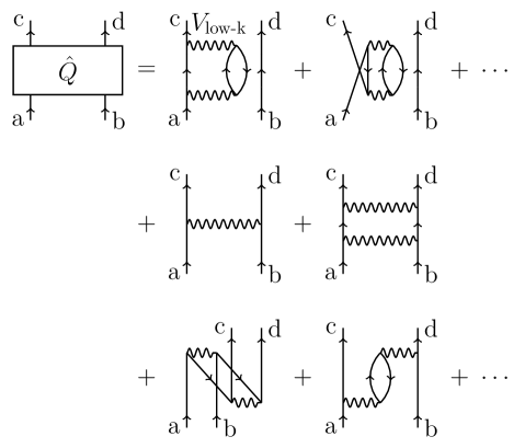
Figure 1: The $\hat{Q}$-box to second order in $V_{{\rm low}\,k}$ (ellipses indicate higher-order terms). The first line contains one-body contributions and the others two-body contributions. Exchange diagrams, though not shown, are included in our calculations.

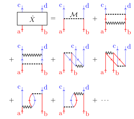
Figure 2: (Color online) The $\hat{X}$-box to first order in $V_{{\rm low}\,k}$. Solid (red) up- or down-going lines indicate neutrons and dotted (blue) lines protons. The wavy horizontal lines, as in Fig. 1, represent $V_{{\rm low}\,k}$, and the dashed horizontal lines represent the $0\nu\beta\beta$-decay operator in Eq. (1).

Figure 3: Diagrams in the expansion of the effective interaction defining the two-body part of the second- and third-order $\hat{Q}$-box. The wavy lines represent $V_{{\rm low}\,k}$. We obtain the first- and second-order $\hat{X}$-box — the set of all unfolded first- and second-order diagrams for the two-body effective operator (not including norm diagrams) — by replacing one interaction in each of these diagrams by a $\beta\beta$-decay operator (in all possible ways) and restricting the sums over nucleons in the intermediate states to either neutrons or protons, as in the first-order $\hat{X}$-box diagrams in Fig. 2.

Folding is significantly more complicated for a two-body transition operator, which combines $\hat{X}$- and $\hat{Q}$-boxes, than for the Hamiltonian, where only $\hat{Q}$-boxes are needed. Effective model-space operators in the basis of energy eigenstates are always defined (for a bare operator $\mathcal{M}$) via

$$\frac{\bra{f_{\text{eff}}}\mathcal{M}_{\text{eff}}\ket{i_{\text{eff}}}}{\braket{f_{\text{eff}}}{f_{\text{eff}}}^{\frac{1}{2}}\braket{i_{\text{eff}}}{i_{\text{eff}}}^{\frac{1}{2}}}=\bra{f}\mathcal{M}\ket{i}\,,$$ (6)

where the states that lie in the model space, $\ket{i_{\text{eff}}}\equiv\hat{P}\ket{i}$ and $\ket{f_{\text{eff}}}\equiv\hat{P}\ket{f}$, are not in general normalized. If $\mathcal{M}$ is the Hamiltonian, then only diagonal matrix elements are nonzero, and the denominator is canceled by a similar factor in the numerator. For two-body transition operators, that is not the case, and state norms must be explicitly computed. Prior authors have approached the issue of norms in several ways. References Brandow (1967) and Ellis (1975), for instance, choose to expand the denominators and fold them into the numerators, thus completely eliminating all disconnected diagrams. The resulting expressions, however, become complicated as the number of folds increases, and the approach requires the construction of a special basis as an intermediate step. For these reasons Ref. Krenciglowa and Kuo (1975) advocates keeping the denominator and numerator separate, at the price of introducing disconnected diagrams that only cancel when the sum is carried out completely. Here, though we evaluate the $\hat{Q}$-box to third order and the $\hat{X}$-box to second order in the interaction, we include only one fold in each of the three factors on the left hand side of Eq. (6), and so opt to follow Refs. Brandow (1967); Krenciglowa and Kuo (1975) in expanding the denominator and folding with the numerator. The resulting expression for the matrix elements of an operator $\mathcal{M}_{\text{eff}}$ is approximately

$$\bra{cd}\mathcal{M}_{\text{eff}}\ket{ab}=$$ (7)

$$\left(\left[1+\frac{1}{2}\frac{d\hat{Q}(\varepsilon)}{d\varepsilon}+\frac{1}{2}\frac{d^{2}\hat{Q}(\varepsilon)}{d^{2}\varepsilon}\hat{Q}(\varepsilon)+\frac{3}{8}\left(\frac{d\hat{Q}(\varepsilon)}{d\varepsilon}\right)^{2}\ldots\right]\right.$$

$$\times\left[\hat{X}(\varepsilon)+\hat{Q}(\varepsilon)\frac{\partial\hat{X}(\varepsilon_{f},\varepsilon)}{\partial\varepsilon_{f}}\bigg{|}_{\varepsilon_{f}=\varepsilon}\!\!\!\!+\frac{\partial\hat{X}(\varepsilon,\varepsilon_{i})}{\partial\varepsilon_{i}}\bigg{|}_{\varepsilon_{i}=\varepsilon}\!\!\!\hat{Q}(\varepsilon)\ldots\right]$$

$$\left.\times\left[1+\frac{1}{2}\frac{d\hat{Q}(\varepsilon)}{d\varepsilon}+\frac{1}{2}\frac{d^{2}\hat{Q}(\varepsilon)}{d^{2}\varepsilon}\hat{Q}(\varepsilon)+\frac{3}{8}\left(\frac{d\hat{Q}(\varepsilon)}{d\varepsilon}\right)^{2}\ldots\right]\right)_{cd,ab}$$

where $\varepsilon$ is the unperturbed energy of both the initial and final states (we take the energies to be the same). Both $\hat{Q}$ and $\hat{X}$ are matrices, with indices corresponding to the possible two-body states in the valence space (e.g., $a,b$ or $c,d$ in Figs. 1 and 2). In this paper we report results of just the terms explicitly given above, which contain between zero and five folds (there is a fold at every matrix multiplication). The terms indicated by ellipses are more complicated and presumably less important; they await future investigation.

II.4 Evaluation of $\hat{Q}$- and $\hat{X}$-Box Diagrams

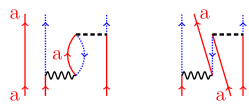
Figure 4: (Color online) A Pauli-forbidden two-body diagram with a spectator neutron and a three-body diagram, obtained by exchanging two ingoing neutron lines, that cancels it exactly.

We turn now to the $\hat{Q}$- and $\hat{X}$-boxes themselves, constructed from unfolded diagrams, that we use in Eq. (7). To construct the $\hat{Q}$-box, we take all unfolded diagrams to third order in $V_{{\rm low}\,k}$. The diagrams appear in Appendix A.2 of Ref. Hjorth-Jensen et al. (1995), and the two-body pieces are reproduced in Fig. 3. Our $\hat{X}$-box has too many diagrams to display here, so we characterize the set as follows: we take all two-body $\hat{Q}$-box diagrams in Fig. 3 and replace one interaction line in each diagram (in all possible ways) by a $\beta\beta$-decay line. We then determine whether each intermediate-state nucleon line should be a proton or neutron. The result is three times as many $\hat{X}$-box diagrams (at second order in $V_{{\rm low}\,k}$) as $\hat{Q}$-box diagrams in Fig. 3.

We make one nonstandard choice in evaluating the $\hat{X}$-box: we restrict the particle lines in the intermediate states to be essentially unoccupied. For example, in the $\beta\beta$ decay of ⁷⁶Ge, we omit all contributions from intermediate protons in the $1p_{3/2}$ orbit and neutrons in $1p_{3/2}$, $1p_{1/2}$, or $0f_{5/2}$ orbits, ad we multiply the contributions of graphs with intermediate neutrons in the $0g_{9/2}$ orbit by 0.4, its average occupancy. In the decay of ⁸²Se, we omit the same contributions as in ⁷⁶Ge and multiply the contributions of graphs with intermediate neutrons in the $0g_{9/2}$ orbit by 0.2 and those with intermediate protons in the $0f_{5/2}$ orbit by 0.5. The reason for all this is that in a nucleus with more than two valence nucleons, the diagram on the left of Fig. 4 — a two-body contribution to the $\beta\beta$-decay operator with a spectator neutron — would be canceled by the three-body diagram on the right if we were to include it. By omitting the two-body diagrams with intermediate particles in occupied orbits we are effectively adding particular three-body diagrams (like those on the right of Fig. 4) to our calculation. We are not including all three-body diagrams, just those that cancel Pauli-forbidden two-body diagrams.

We call this approach nonstandard because it is not usually followed in derivations of effective interactions. The reason is that in excluding some Pauli-forbidden diagrams, one effectively includes unlinked one- and two-body diagrams (see, e.g., Fig. 10 of Ref. Ellis and Osnes (1977)) as well as the exclusion-enforcing three-body diagrams we want. This problem, however, is more pronounced in the $\hat{Q}$-box than the $\hat{X}$-box since the latter has no one-body part and far fewer ways to unlink diagrams by exchanging lines (the horizontal $\beta\beta$-decay lines are restricted to have incoming neutrons and outgoing protons). We therefore effectively include only very few unlinked diagrams by introducing our restrictions in the $\hat{X}$-box; the compensating benefit is a much better account of Pauli exclusion, an important physical effect. Diagrams such as the one on the left of Fig. 4 result in large contributions that should not be present in a full calculation. We cancel them with the implicit assumption that the canceling contribution from the figure on the right-hand side is significantly greater than that of typical third-order diagrams, which we omit. Eventually, though, this assumption will have to be tested explicitly.

III Results

	76Ge	82Se
Bare matrix element $M_{0\nu}$	3.12	2.73
First-order $\hat{X}$-box, without 3p-1h	5.44	4.86
Full first-order $\hat{X}$-box	2.20	2.40
First order folded	3.11	2.79
Full second-order $\hat{X}$-box	4.14	3.92
Final matrix element	3.77	3.62
CD-Bonn $G$-matrix	3.62	3.45
N3LO $G$-matrix	3.48	3.33

Table 1: The $0\nu\beta\beta$-decay matrix elements $M_{0\nu}$ for ⁷⁶Ge and ⁸²Se at various approximations in our many-body framework.

To obtain our final corrected shell-model $0\nu\beta\beta$-decay matrix elements, we combine the individual two-body matrix elements of our effective operator with two-body shell-model transition densities. Since our aim is a consistent calculation without empirical adjustment, we really ought to take two-body densities from the diagonalization of a valence-space interaction that is derived directly from NN+3N forces. While work in this direction is in progress, the computation is not yet possible in nuclei this heavy. Instead we use two-body densities from existing shell-model calculations, the interactions for which have been tweaked to fit experimental data in nearby nuclei. For ⁷⁶Ge we use the calculation of Horoi Horoi (2012) and for ⁸²Se that of Ref. Menéndez et al. (2009); the authors of both have kindly supplied us with their transition densities.

Table 1 presents our matrix elements at various levels of $\hat{X}$-box and folding approximations, using $V_{{\rm low}\,k}$ and taking intermediate-state excitations to $18\hbar\omega$. Despite differences in the NN interaction and size of the basis space, contributions from first-order diagrams in both ⁷⁶Ge and ⁸²Se largely agree with those first identified in Ref. Engel and Hagen (2009): particle-particle and hole-hole ladders together enhance the matrix element, while the three-particle one-hole diagrams cause a dramatic reduction. When folding is included, however, the net correction from first-order $\hat{Q}$- and $\hat{X}$-boxes essentially disappears. Taking the complete set of second-order diagrams into account, we find a significant enhancement followed by a modest quenching from folding. The final matrix element is approximately 20% percent larger than the bare matrix element in ⁷⁶Ge and about 30% larger in ⁸²Se. The primary reason for the different effects in ⁸²Se and ⁷⁶Ge is the difference in the omitted intermediate-state orbits discussed in Section II.4. If we include those orbits, as is standard practice in the construction of effective interactions, the matrix element is reduced by about 10% in ⁷⁶Ge and 15% in ⁸²Se. In Ref. Lincoln et al. (2013), which contains a preliminary account of our calculations in ⁸²Se, we obtained 3.56 instead of 3.62. The small difference is due to the inclusion in Ref. Lincoln et al. (2013) of $\hat{Q}$-box restrictions and the addition here of a term in the expansion of the norm denominator. Though the two results are close, we believe that the one reported here is likely closer to the real matrix element.

	$8\hbar\omega$	$10\hbar\omega$	$12\hbar\omega$	$14\hbar\omega$	$16\hbar\omega$	$18\hbar\omega$
Full 1st order	$2.429$	$2.407$	$2.403$	$2.401$	$2.399$	$2.399$
Full 2nd order	$3.908$	$3.932$	$3.940$	$3.931$	$3.925$	$3.924$
Final	$3.489$	$3.553$	$3.595$	$3.611$	$3.617$	$3.618$

Table 2: Convergence of $0\nu\beta\beta$-decay matrix element in ⁸²Se with respect to allowed intermediate-state excitations. In all cases we work in a harmonic-oscillator basis of 13 major shells.

Several other aspects of the calculation are robust. As seen in Table 2, our $V_{{\rm low}\,k}$ results at $18\hbar\omega$ are well converged to 3 or 4 digits. And as Table 1 shows, changing the interaction to a $G$-matrix (in 11 major oscillator shells) in place of $V_{{\rm low}\,k}$ does not affect the results substantially. Finally, although we emphasized our procedure of requiring intermediate-particle lines in $\hat{X}$-box diagrams to be unoccupied in the nucleus in question, other prescriptions yield similar results once norms and folding are included: in ⁸²Se, for example, we obtain a final matrix element of 3.50 if we restrict particle lines in both the $\hat{Q}$ and $\hat{X}$ boxes, and 3.03 if we impose no restrictions at all. We should note, however, that at various intermediate stages of the calculation, the procedures yield quite different results. And other parts of the calculation leave room for change as more physics is included.

	Restricted	Unrestricted
Bare matrix element $M^{\rm cl}_{2\nu}$	0.57	0.57
First-order $\hat{X}$-box, without 3p-1h	0.99	0.89
Full first-order $\hat{X}$-box	0.37	-0.60
Full second-order $\hat{X}$-box	0.79	-0.37
Final matrix element	0.96	0.70

Table 3: The $2\nu\beta\beta$-decay closure matrix $M_{2\nu}^{\text{cl}}$ for ⁷⁶Ge at several levels of approximation, with and without restrictions on occupied intermediate-particle lines.

We turn now to a discussion of $2\nu\beta\beta$ decay. As noted above, we use the closure matrix element $M_{2\nu}^{\text{cl}}$ as a proxy for the full matrix element, a step that limits how much we can say. Table 3 shows the matrix element for ⁷⁶Ge with and without the intermediate-state restrictions we impose on occupied or partially occupied orbits in calculating $M_{0\nu}$. Imposing the restrictions here increases the matrix element, as in $0\nu\beta\beta$ decay; in this case, however, the result is probably undesirable, given that shell model calculations of $2\nu\beta\beta$ decay in ⁷⁶Ge overestimate $M_{2\nu}$. On the other hand, omitting the restrictions increases the negative contribution of the 3p-1h diagram to such an extent that the matrix element changes sign. The sign is eventually reversed by higher-order contributions and folding, ultimately yielding a result that is approximately unchanged from the bare matrix element. It is difficult to be comfortable, however, with a low-order correction that changes the sign of the matrix element. The sensitivity of the numbers suggest that terms with more folds, of higher order, or involving more valence orbitals could also have a significant effect.

Another reason (aside from the sign changes in the right-hand column of Table 3) for preferring to restrict intermediate-sate orbits in the $\hat{X}$-box is connected to the long-standing problem of the apparent suppression of the axial-vector coupling constant $g_{A}$ in the nuclear medium Towner (1987). While the suppression probably has many sources, configurations outside the valence space are likely to play a key role. Though the bare operator governing weak decay is one-body, we can simulate the effect of $g_{A}$ suppression in $2\nu\beta\beta$ decay by including only closure diagrams that have the form shown in Fig. 5. Such diagrams, in which only a single $2\nu\beta\beta$-decay line connects the two nucleons, incorporates only the renormalization of the one-body weak current.

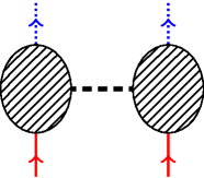
Figure 5: (Color online) Schematic representation of diagrams contributing to renormalization of $g_{A}$ in $2\nu\beta\beta$ decay.

When we base our calculation of $M_{2\nu}^{\text{cl}}$ on only these diagrams and at the same time account for occupied intermediate-state orbits, we find in ⁸²Se that the full result is smaller than the bare result by 38%, implying an effective $g_{A}$ of about 1.0, a reasonable value (in ⁷⁶Ge the value is about 0.7). On the other hand, when we take no account of occupied orbits we find (again, with only diagrams of the form in Fig. 5 included) that the closure matrix element changes sign, something that is impossible through the renormalization of $g_{A}$ alone. The sign change reflects the same strong effect of the 3p-1h diagrams observed in Table 3. Though these considerations are not conclusive, they do indicate that taking the Pauli principle into account is a beneficial. Work is currently underway to investigate $g_{A}$ quenching more directly. By focusing on the one-body operator, we can use analogous many-body techniques, based again on chiral NN and 3N physics, with the effects of two-body currents implemented consistently in the bare operator Menéndez et al. (2011) to understand the origin of $g_{A}$ quenching.

Whatever the outcome of that investigation, it is clear that the $2\nu\beta\beta$ matrix element is sensitive to many details in the wavefunctions, much more sensitive than its $0\nu\beta\beta$ counterpart. Thus, although the increase of the $2\nu\beta\beta$ closure matrix element does not bolster the case for our $0\nu\beta\beta$ calculation, neither, in our view, does it weaken it much.

IV Discussion and Outlook

We have used chiral nuclear forces and many-body perturbation theory to calculate an effective shell-model $0\nu\beta\beta$-decay operator, taking into account corrections to the bare operator from configurations outside the valence to second order in the interaction. The resulting nuclear matrix element is approximately 20% larger than the bare matrix element in ⁷⁶Ge and about 30% larger in ⁸²Se. These new results represent our current best estimates for the matrix elements but probably do not tell the whole story. We have omitted a number of effects that could further alter the results. To do better, we must first establish consistency between the Hamiltonian and our effective operator. This will require the construction of full non-empirical valence-space interactions in the $pf$ shell from NN and 3N forces; work in that direction is in progress. A related improvement will be to include the effects of chiral 3N forces in the $\hat{X}$-box, in addition to the effects of chiral two-body currents in the bare operator Menéndez et al. (2011).

At the many-body level, the importance of third- and higher-order terms in the $\hat{X}$-box and additional folding contributions must be understood. Since we have found the effects of bubble diagrams to be the most important in our perturbative expansion, it would be worthwhile to pursue a nonperturbative calculation of the effects of core polarization (which these diagrams represent), like that done for effective interactions in Ref. Holt et al. (2005). Perhaps the most significant obstacle to a truly reliable result, however, is the implementation of induced three-body operators. Recent work Shukla et al. (2011); Engel and Vogel (2004) indicates that such operators are not negligible, and even here we have shown that three-body diagrams of the form in Fig. 4 are important. Unfortunately, the number of induced three-body diagrams is so large that nobody has computed them even in the construction of effective interactions. We must find a way to at least estimate their size if we want to pursue perturbation theory to its conclusion. Controlled nonperturbative approaches Tsukiyama et al. (2012); Jansen et al. (2011) are on the horizon, but the inclusion of induced three-body terms is technically difficult there as well. In none of these approaches is the problem impossible to overcome, but doing so will require diligence and creativity.