A Spectral Analysis of Subspace Enchanced Preconditioners

Tao Zhao Department of Computer Science, University of Colorado Boulder, CO 80309, USA (tao.zhao@colorado.edu)
Abstract

It is well-known that the convergence of Krylov subspace methods to solve linear system depends on the spectrum of the coefficient matrix, moreover, it is widely accepted that for both symmetric and unsymmetric systems Krylov subspace methods will converge fast if the spectrum of the coefficient matrix is clustered. In this paper we investigate the spectrum of the system preconditioned by the deflation, coarse correction and adapted deflation preconditioners. Our analysis shows that the spectrum of the preconditioned system is highly impacted by the angle between the coarse space for the construction of the three preconditioners and the subspace spanned by the eigenvectors associated with the small eigenvalues of the coefficient matrix. Furthermore, we prove that the accuracy of the inverse of projection matrix also impacts the spectrum of the preconditioned system. Numerical experiments emphasized the theoretical analysis.

keywords:
spectrum, coarse space, deflation, preconditioner, perturbation analysis, projection matrix, iterative solvers, domain decomposition

1 Introduction

We consider the iterative solution of a linear system

Ax=b,𝐴𝑥𝑏Ax=b,

where An×n𝐴superscript𝑛𝑛A\in\mathbb{R}^{n\times n} is symmetric and positive definite (SPD). It is well-known that the convergence of Krylov subspace methods for solving linear systems depend on the eigenvalue distribution of A𝐴A. Recently, several studies [11, 8, 19, 14, 10, 13, 2, 3, 12, 5, 7] have shown that by removing the subspace spanned by the eigenvectors corresponding to several small eigenvalues from the Krylov search space makes the spectrum more clustered and consequently the convergence is improved.

In this paper, we refer to matrix of the form

E=ZTAZ,Zn×r.formulae-sequence𝐸superscript𝑍𝑇𝐴𝑍𝑍superscript𝑛𝑟\displaystyle E=Z^{T}AZ,~{}~{}Z\in\mathbb{R}^{n\times r}. (1)

as a projection matrix, and the subspace spanned by the columns of Z𝑍Z is referred to as a coarse space. In an ideal situation, the coarse space contains the vectors corresponding to the lower part of the spectrum that is responsible for the stagnation of Krylov subspace methods. As shown in this paper, the preconditioned systems will have the desired properties when the preconditioner is enchanced with the ideal coarse subspace. In contrast to the general coarse space, we refer to the coarse space spanned by the eigenvectors associated with several small eigenvalues of A𝐴A as the exact coarse space.

Next we briefly mention a few existing approaches that take the form of a standard precondition with an additive coarse space enchancement. In [3, 12], the deflation preconditioner is defined by

PD=IAZE1ZT.subscript𝑃𝐷𝐼𝐴𝑍superscript𝐸1superscript𝑍𝑇\displaystyle P_{D}=I-AZE^{-1}Z^{T}. (2)

Obviously PDAsubscript𝑃𝐷𝐴P_{D}A is singular since PDsubscript𝑃𝐷P_{D} is singular. Fortunately, Krylov subspace methods converge for singular linear systems as long as they are consistent; furthermore, zero eigenvalues do not impact the convergence since the corresponding eigenvectors never enter the Krylov subspace [12].

Instead of zero out the small eigenspace in the deflation method, the preconditioners based on coarse correction shift the small eigenvalues to the large ones. In [19], the coarse correction preconditioner in domain decomposition method is defined by

PC=I+ZE1ZT.subscript𝑃𝐶𝐼𝑍superscript𝐸1superscript𝑍𝑇\displaystyle P_{C}=I+ZE^{-1}Z^{T}. (3)

The abstract additive coarse correction is M1+ZE1ZTsuperscript𝑀1𝑍superscript𝐸1superscript𝑍𝑇M^{-1}+ZE^{-1}Z^{T}, where M𝑀M is the sum of the local solves in each subdomain. Another popular preconditioner in domain decomposition method is the abstract balancing preconditioner [3]

PBNN=(IZE1ZTA)M1(IAZE1ZT)+ZE1ZT.subscript𝑃𝐵𝑁𝑁𝐼𝑍superscript𝐸1superscript𝑍𝑇𝐴superscript𝑀1𝐼𝐴𝑍superscript𝐸1superscript𝑍𝑇𝑍superscript𝐸1superscript𝑍𝑇\displaystyle P_{BNN}=(I-ZE^{-1}Z^{T}A)M^{-1}(I-AZE^{-1}Z^{T})+ZE^{-1}Z^{T}. (4)

The adapted deflation preconditioner [19] is defined as

PADEF1=M1PD+ZE1ZT.subscript𝑃𝐴𝐷𝐸𝐹1superscript𝑀1subscript𝑃𝐷𝑍superscript𝐸1superscript𝑍𝑇\displaystyle P_{ADEF1}=M^{-1}P_{D}+ZE^{-1}Z^{T}.

It is shown in [19] that PADEF1subscript𝑃𝐴𝐷𝐸𝐹1P_{ADEF1} is cheaper than PBNNsubscript𝑃𝐵𝑁𝑁P_{BNN} but is as robust as PBNNsubscript𝑃𝐵𝑁𝑁P_{BNN}. Moreover, PBNNAsubscript𝑃𝐵𝑁𝑁𝐴P_{BNN}A and PADEF1Asubscript𝑃𝐴𝐷𝐸𝐹1𝐴P_{ADEF1}A have an identical spectrum. In both PBNNsubscript𝑃𝐵𝑁𝑁P_{BNN} and PADEF1subscript𝑃𝐴𝐷𝐸𝐹1P_{ADEF1}, the first term corresponds to the fine space and the second term is for the coarse space, therefore they are called two-level preconditioners. Throughout this paper, we restrict our analysis to one-level methods. Let M𝑀M in PADEF1subscript𝑃𝐴𝐷𝐸𝐹1P_{ADEF1} be I𝐼I. We define PAsubscript𝑃𝐴P_{A} as

PA=IAZE1ZT+ZE1ZT.subscript𝑃𝐴𝐼𝐴𝑍superscript𝐸1superscript𝑍𝑇𝑍superscript𝐸1superscript𝑍𝑇\displaystyle P_{A}=I-AZE^{-1}Z^{T}+ZE^{-1}Z^{T}. (5)

Let X𝑋X be any basis of a coarse space not Z𝑍Z. Obviously the following identity

X(XTAX)1XT=Z(ZTAZ)1ZT𝑋superscriptsuperscript𝑋𝑇𝐴𝑋1superscript𝑋𝑇𝑍superscriptsuperscript𝑍𝑇𝐴𝑍1superscript𝑍𝑇X(X^{T}AX)^{-1}X^{T}=Z(Z^{T}AZ)^{-1}Z^{T}

holds in exact arithmetic since there exists a nonsingular matrix Cr×r𝐶superscript𝑟𝑟C\in\mathbb{R}^{r\times r} such that X=ZC𝑋𝑍𝐶X=ZC. This implies that PDsubscript𝑃𝐷P_{D}, PCsubscript𝑃𝐶P_{C} and PAsubscript𝑃𝐴P_{A} are determined uniquely by the coarse space. Thus we can choose an appropriate basis to form Z𝑍Z and then to construct a preconditioner with certain desirable properties.

As we will see, if an approximate coarse space is used to construct preconditioners, then the spectrum of the preconditioned systems is related to the angle between the approximate and exact coarse spaces. We also prove that the coarse correction and adapted deflation preconditioners are more roust than the deflation preconditioner when the projection matrix is solved inexactly. In section 2, we first review the spectral properties of the preconditioned system when the preconditioners are constructed with the exact coarse space, then we estimate the spectral bounds of the preconditioned systems when the approximate coarse space is used. Section 3 presents the perturbation analysis on the spectrum of the preconditioned system in the case that the projection matrix have some perturbation. Numerical results are reported in Section 4.

2 Coarse space spanned by the approximate coarse space

In this section, we briefly review the spectrum of the system preconditioned by using the exact coarse space, then based on these properties we derive the bounds of the spectrum of the system preconditioned by using the approximate coarse space. Let (λi,vi)subscript𝜆𝑖subscript𝑣𝑖(\lambda_{i},v_{i}) be an eigenpair of A𝐴A and visubscript𝑣𝑖v_{i} be normalized. (vi,,vn)subscript𝑣𝑖subscript𝑣𝑛(v_{i},\cdots,v_{n}) is orthogonal since A𝐴A is SPD. The spectral decomposition of A𝐴A can be written as

A=(V,V)(Λ00Λ)(VTVT),𝐴𝑉subscript𝑉perpendicular-toΛ00subscriptΛperpendicular-tosuperscript𝑉𝑇subscriptsuperscript𝑉𝑇perpendicular-to\displaystyle A=(V,V_{\perp})\left(\begin{array}[]{cc}\Lambda&0\\ 0&\Lambda_{\perp}\end{array}\right)\left(\begin{array}[]{c}V^{T}\\ V^{T}_{\perp}\end{array}\right), (10)

where Λ=diag{λ1,,λr}Λ𝑑𝑖𝑎𝑔subscript𝜆1subscript𝜆𝑟\Lambda=diag\{\lambda_{1},\cdots,\lambda_{r}\}, Λ=diag{λr+1,,λn}subscriptΛperpendicular-to𝑑𝑖𝑎𝑔subscript𝜆𝑟1subscript𝜆𝑛\Lambda_{\perp}=diag\{\lambda_{r+1},\cdots,\lambda_{n}\}, V=(v1,,vr)𝑉subscript𝑣1subscript𝑣𝑟V=(v_{1},\cdots,v_{r}), and V=(vr+1,,vn)subscript𝑉perpendicular-tosubscript𝑣𝑟1subscript𝑣𝑛V_{\perp}=(v_{r+1},\cdots,v_{n}).

Assume that λ1subscript𝜆1\lambda_{1}, λ2subscript𝜆2\lambda_{2}, \cdots, λrsubscript𝜆𝑟\lambda_{r} are small eigenvalues that impacts the convergence of the Krylov subspace methods. Theorem 1 and Theorem 2 show that if we take Z=V𝑍𝑉Z=V, the small eigenvalues are removed or shifted when the preconditioners are applied on either side of A𝐴A, moreover, the rest of eigenvalues and all the eigenvectors are not changed.

Theorem 1.

Let E~=VTAV~𝐸superscript𝑉𝑇𝐴𝑉\tilde{E}=V^{T}AV. Define

P~Dsubscript~𝑃𝐷\displaystyle\tilde{P}_{D} =\displaystyle= IAVE~1VT,𝐼𝐴𝑉superscript~𝐸1superscript𝑉𝑇\displaystyle I-AV\tilde{E}^{-1}V^{T},
P~Csubscript~𝑃𝐶\displaystyle\tilde{P}_{C} =\displaystyle= I+VE~1VT,𝐼𝑉superscript~𝐸1superscript𝑉𝑇\displaystyle I+V\tilde{E}^{-1}V^{T},
P~Asubscript~𝑃𝐴\displaystyle\tilde{P}_{A} =\displaystyle= IAVE~1VT+VE~1VT.𝐼𝐴𝑉superscript~𝐸1superscript𝑉𝑇𝑉superscript~𝐸1superscript𝑉𝑇\displaystyle I-AV\tilde{E}^{-1}V^{T}+V\tilde{E}^{-1}V^{T}.

Then we have the following spectral decomposition

P~DAsubscript~𝑃𝐷𝐴\displaystyle\tilde{P}_{D}A =\displaystyle= (V,V)(000Λ)(VTVT),𝑉subscript𝑉perpendicular-to000subscriptΛperpendicular-tosuperscript𝑉𝑇subscriptsuperscript𝑉𝑇perpendicular-to\displaystyle(V,V_{\perp})\left(\begin{array}[]{cc}0&0\\ 0&\Lambda_{\perp}\end{array}\right)\left(\begin{array}[]{c}V^{T}\\ V^{T}_{\perp}\end{array}\right),
P~CAsubscript~𝑃𝐶𝐴\displaystyle\tilde{P}_{C}A =\displaystyle= (V,V)(I+Λ00Λ)(VTVT),𝑉subscript𝑉perpendicular-to𝐼Λ00subscriptΛperpendicular-tosuperscript𝑉𝑇subscriptsuperscript𝑉𝑇perpendicular-to\displaystyle(V,V_{\perp})\left(\begin{array}[]{cc}I+\Lambda&0\\ 0&\Lambda_{\perp}\end{array}\right)\left(\begin{array}[]{c}V^{T}\\ V^{T}_{\perp}\end{array}\right),
P~AAsubscript~𝑃𝐴𝐴\displaystyle\tilde{P}_{A}A =\displaystyle= (V,V)(I00Λ)(VTVT).𝑉subscript𝑉perpendicular-to𝐼00subscriptΛperpendicular-tosuperscript𝑉𝑇subscriptsuperscript𝑉𝑇perpendicular-to\displaystyle(V,V_{\perp})\left(\begin{array}[]{cc}I&0\\ 0&\Lambda_{\perp}\end{array}\right)\left(\begin{array}[]{c}V^{T}\\ V^{T}_{\perp}\end{array}\right).
Proof.

From the definition of E~~𝐸\tilde{E}, we have

E~=VTAV=VTVΛ=Λ.~𝐸superscript𝑉𝑇𝐴𝑉superscript𝑉𝑇𝑉ΛΛ\tilde{E}=V^{T}AV=V^{T}V\Lambda=\Lambda.

Next, let us consider the first result. Obviously, P~DAV=0subscript~𝑃𝐷𝐴𝑉0\tilde{P}_{D}AV=0. We then have

P~DAVsubscript~𝑃𝐷𝐴subscript𝑉perpendicular-to\displaystyle\tilde{P}_{D}AV_{\perp} =\displaystyle= AVAVΛ1VTAV𝐴subscript𝑉perpendicular-to𝐴𝑉superscriptΛ1superscript𝑉𝑇𝐴subscript𝑉perpendicular-to\displaystyle AV_{\perp}-AV\Lambda^{-1}V^{T}AV_{\perp}
=\displaystyle= VΛVVTVΛsubscript𝑉perpendicular-tosubscriptΛperpendicular-to𝑉superscript𝑉𝑇subscript𝑉perpendicular-tosubscriptΛperpendicular-to\displaystyle V_{\perp}\Lambda_{\perp}-VV^{T}V_{\perp}\Lambda_{\perp}
=\displaystyle= VΛ.subscript𝑉perpendicular-tosubscriptΛperpendicular-to\displaystyle V_{\perp}\Lambda_{\perp}.

Thus the first spectral decomposition holds. Since

P~CA=A+AVE~1VT=A+VΛΛ1VT=A+VVT,subscript~𝑃𝐶𝐴𝐴𝐴𝑉superscript~𝐸1superscript𝑉𝑇𝐴𝑉ΛsuperscriptΛ1superscript𝑉𝑇𝐴𝑉superscript𝑉𝑇\displaystyle\tilde{P}_{C}A=A+AV\tilde{E}^{-1}V^{T}=A+V\Lambda\Lambda^{-1}V^{T}=A+VV^{T},

we have

P~CAV=AV+VVTV=V(Λ+I)subscript~𝑃𝐶𝐴𝑉𝐴𝑉𝑉superscript𝑉𝑇𝑉𝑉Λ𝐼\tilde{P}_{C}AV=AV+VV^{T}V=V(\Lambda+I)

and

P~CAV=AV+VVTV=AV=Vλ.subscript~𝑃𝐶𝐴subscript𝑉perpendicular-to𝐴subscript𝑉perpendicular-to𝑉superscript𝑉𝑇subscript𝑉perpendicular-to𝐴subscript𝑉perpendicular-tosubscript𝑉perpendicular-tosubscript𝜆perpendicular-to\tilde{P}_{C}AV_{\perp}=AV_{\perp}+VV^{T}V_{\perp}=AV_{\perp}=V_{\perp}\lambda_{\perp}.

Hence, the second spectral decomposition is true. The third spectral decomposition follows from

P~AAV=AVAVE~1VTAV+VE~1VTAV=Vsubscript~𝑃𝐴𝐴𝑉𝐴𝑉𝐴𝑉superscript~𝐸1superscript𝑉𝑇𝐴𝑉𝑉superscript~𝐸1superscript𝑉𝑇𝐴𝑉𝑉\tilde{P}_{A}AV=AV-AV\tilde{E}^{-1}V^{T}AV+V\tilde{E}^{-1}V^{T}AV=V

and

P~AAVsubscript~𝑃𝐴𝐴subscript𝑉perpendicular-to\displaystyle\tilde{P}_{A}AV_{\perp} =\displaystyle= AVAVE~1VTAV+VE~1VTAV𝐴subscript𝑉perpendicular-to𝐴𝑉superscript~𝐸1superscript𝑉𝑇𝐴subscript𝑉perpendicular-to𝑉superscript~𝐸1superscript𝑉𝑇𝐴subscript𝑉perpendicular-to\displaystyle AV_{\perp}-AV\tilde{E}^{-1}V^{T}AV_{\perp}+V\tilde{E}^{-1}V^{T}AV_{\perp}
=\displaystyle= AVAVE~1VTVΛ+VE~1VTVΛ𝐴subscript𝑉perpendicular-to𝐴𝑉superscript~𝐸1superscript𝑉𝑇subscript𝑉perpendicular-tosubscriptΛperpendicular-to𝑉superscript~𝐸1superscript𝑉𝑇subscript𝑉perpendicular-tosubscriptΛperpendicular-to\displaystyle AV_{\perp}-AV\tilde{E}^{-1}V^{T}V_{\perp}\Lambda_{\perp}+V\tilde{E}^{-1}V^{T}V_{\perp}\Lambda_{\perp}
=\displaystyle= AV=VΛ𝐴subscript𝑉perpendicular-tosubscript𝑉perpendicular-tosubscriptΛperpendicular-to\displaystyle AV_{\perp}=V_{\perp}\Lambda_{\perp}

It follows immediately from these three spectral decomposition that PDAsubscript𝑃𝐷𝐴P_{D}A, PCAsubscript𝑃𝐶𝐴P_{C}A and PAAsubscript𝑃𝐴𝐴P_{A}A are symmetric. ∎

Theorem 2.

P~Dsubscript~𝑃𝐷\tilde{P}_{D}, P~Csubscript~𝑃𝐶\tilde{P}_{C} and P~Asubscript~𝑃𝐴\tilde{P}_{A} are defined in Theorem 1. Then we have AP~D=P~DA𝐴subscript~𝑃𝐷subscript~𝑃𝐷𝐴A\tilde{P}_{D}=\tilde{P}_{D}A, AP~C=P~CA𝐴subscript~𝑃𝐶subscript~𝑃𝐶𝐴A\tilde{P}_{C}=\tilde{P}_{C}A and AP~A=P~AA𝐴subscript~𝑃𝐴subscript~𝑃𝐴𝐴A\tilde{P}_{A}=\tilde{P}_{A}A.

Proof.

The first result follows from

AP~DV=AVAVΛΛ1VTV=0=P~DAV𝐴subscript~𝑃𝐷𝑉𝐴𝑉𝐴𝑉ΛsuperscriptΛ1superscript𝑉𝑇𝑉0subscript~𝑃𝐷𝐴𝑉A\tilde{P}_{D}V=AV-AV\Lambda\Lambda^{-1}V^{T}V=0=\tilde{P}_{D}AV

and

AP~DV=AV+AVΛ1VTV=VΛ=P~DAV.𝐴subscript~𝑃𝐷subscript𝑉perpendicular-to𝐴subscript𝑉perpendicular-to𝐴𝑉superscriptΛ1superscript𝑉𝑇subscript𝑉perpendicular-tosubscript𝑉perpendicular-tosubscriptΛperpendicular-tosubscript~𝑃𝐷𝐴subscript𝑉perpendicular-toA\tilde{P}_{D}V_{\perp}=AV_{\perp}+AV\Lambda^{-1}V^{T}V_{\perp}=V_{\perp}\Lambda_{\perp}=\tilde{P}_{D}AV_{\perp}.

Note that A𝐴A, P~Csubscript~𝑃𝐶\tilde{P}_{C} and P~CAsubscript~𝑃𝐶𝐴\tilde{P}_{C}A are symmetric. We then have

P~CA=(P~CA)T=ATP~CT=AP~C.subscript~𝑃𝐶𝐴superscriptsubscript~𝑃𝐶𝐴𝑇superscript𝐴𝑇subscriptsuperscript~𝑃𝑇𝐶𝐴subscript~𝑃𝐶\tilde{P}_{C}A=(\tilde{P}_{C}A)^{T}=A^{T}\tilde{P}^{T}_{C}=A\tilde{P}_{C}.

Since

AP~A𝐴subscript~𝑃𝐴\displaystyle A\tilde{P}_{A} =\displaystyle= AA2VE~1VT+AVE~1VT𝐴superscript𝐴2𝑉superscript~𝐸1superscript𝑉𝑇𝐴𝑉superscript~𝐸1superscript𝑉𝑇\displaystyle A-A^{2}V\tilde{E}^{-1}V^{T}+AV\tilde{E}^{-1}V^{T}
=\displaystyle= AAVΛΛ1VT+VΛΛ1VT𝐴𝐴𝑉ΛsuperscriptΛ1superscript𝑉𝑇𝑉ΛsuperscriptΛ1superscript𝑉𝑇\displaystyle A-AV\Lambda\Lambda^{-1}V^{T}+V\Lambda\Lambda^{-1}V^{T}
=\displaystyle= AAVVT+VVT,𝐴𝐴𝑉superscript𝑉𝑇𝑉superscript𝑉𝑇\displaystyle A-AVV^{T}+VV^{T},

we get

AP~AV=AVAVVTV+VVTV=V=P~AAV𝐴subscript~𝑃𝐴𝑉𝐴𝑉𝐴𝑉superscript𝑉𝑇𝑉𝑉superscript𝑉𝑇𝑉𝑉subscript~𝑃𝐴𝐴𝑉A\tilde{P}_{A}V=AV-AVV^{T}V+VV^{T}V=V=\tilde{P}_{A}AV

and

AP~AV=AV+AVVTV+VVTV=AV=VΛ=P~AAV.𝐴subscript~𝑃𝐴subscript𝑉perpendicular-to𝐴subscript𝑉perpendicular-to𝐴𝑉superscript𝑉𝑇subscript𝑉perpendicular-to𝑉superscript𝑉𝑇subscript𝑉perpendicular-to𝐴subscript𝑉perpendicular-tosubscript𝑉perpendicular-tosubscriptΛperpendicular-tosubscript~𝑃𝐴𝐴subscript𝑉perpendicular-toA\tilde{P}_{A}V_{\perp}=AV_{\perp}+AVV^{T}V_{\perp}+VV^{T}V_{\perp}=AV_{\perp}=V_{\perp}\Lambda_{\perp}=\tilde{P}_{A}AV_{\perp}.

The third result is therefore true. In addition, APD𝐴subscript𝑃𝐷AP_{D}, APC𝐴subscript𝑃𝐶AP_{C} and APA𝐴subscript𝑃𝐴AP_{A} are symmetric as well. ∎

For a large system, it is impractical to build the preconditioners by using the exact eigenvectors associated with the small eigenvalues, since in general computing these eigenvectors is more costly and more difficult than solving a linear system. Nevertheless, for some cases, the approximate eigenvectors are cheaply obtained and thus are used to produce the preconditioners. For example, in the Newton method for solving nonlinear problems, the information obtained during solving the first linear system is reused to build the coarse spaces for accelerating the convergence of the succeeding linear systems, see [7] and [8]. We hope that the system preconditioned by using the approximate coarse space has the similar eigenvalue distribution as described in Theorem 1. This motivates us to analyse how the perturbation in the coarse space impacts the spectrum of the system preconditioned by PDsubscript𝑃𝐷P_{D}, PCsubscript𝑃𝐶P_{C} and PAsubscript𝑃𝐴P_{A}.

In the following discussion we assume that Z𝑍Z is column orthogonal. Let 𝒵𝒵\mathcal{Z} be the subspace spanned by the columns of Z𝑍Z. Let 𝒵superscript𝒵perpendicular-to\mathcal{Z}^{\perp} be the orthogonal complement of 𝒵𝒵\mathcal{Z} and Zsubscript𝑍perpendicular-toZ_{\perp} be an orthogonal basis of 𝒵superscript𝒵perpendicular-to\mathcal{Z}^{\perp}. Likewise, let 𝒱𝒱\mathcal{V} be the subspace spanned by the columns of V𝑉V, 𝒱superscript𝒱perpendicular-to\mathcal{V}^{\perp} be the orthogonal complement of 𝒱𝒱\mathcal{V} and Vsubscript𝑉perpendicular-toV_{\perp} be an orthogonal basis of 𝒱superscript𝒱perpendicular-to\mathcal{V}^{\perp}. Let σ𝜎\sigma denote the singular value of a matrix. Let dist(𝒵,𝒱)𝑑𝑖𝑠𝑡𝒵𝒱dist(\mathcal{Z},\mathcal{V}) denote the distance between subspaces 𝒵𝒵\mathcal{Z} and 𝒱𝒱\mathcal{V}. It is shown in [6] that dist(𝒵,𝒱)𝑑𝑖𝑠𝑡𝒵𝒱dist(\mathcal{Z},\mathcal{V}) can be evaluated by either σmax(ZTV)subscript𝜎𝑚𝑎𝑥superscript𝑍𝑇subscript𝑉perpendicular-to\sigma_{max}(Z^{T}V_{\perp}) or σmax(VTZ)subscript𝜎𝑚𝑎𝑥superscript𝑉𝑇subscript𝑍perpendicular-to\sigma_{max}(V^{T}Z_{\perp}). Note that 0dist(𝒵,𝒱)10𝑑𝑖𝑠𝑡𝒵𝒱10\leq dist(\mathcal{Z},\mathcal{V})\leq 1 since 𝒵𝒵\mathcal{Z} and 𝒱𝒱\mathcal{V} have the same dimension. We define the acute angle between subspaces 𝒵𝒵\mathcal{Z} and 𝒱𝒱\mathcal{V} as θ=arcsindist(𝒵,𝒱)𝜃𝑑𝑖𝑠𝑡𝒵𝒱\theta=\arcsin dist(\mathcal{Z},\mathcal{V}). The next lemma shows that cosθ𝜃\cos\theta can be evaluated in a similar way as sinθ𝜃\sin\theta.

Lemma 3.

Let θ𝜃\theta be the acute angle between subspaces 𝒵𝒵\mathcal{Z} and 𝒱𝒱\mathcal{V} that have the same dimension. Let Z𝑍Z and V𝑉V be the orthogonal bases of 𝒵𝒵\mathcal{Z} and 𝒱𝒱\mathcal{V} respectively. Then

sinθ𝜃\displaystyle\sin\theta =\displaystyle= σmax(ZTV)=σmax(VTZ),subscript𝜎𝑚𝑎𝑥superscript𝑍𝑇subscript𝑉perpendicular-tosubscript𝜎𝑚𝑎𝑥superscript𝑉𝑇subscript𝑍perpendicular-to\displaystyle\sigma_{max}(Z^{T}V_{\perp})=\sigma_{max}(V^{T}Z_{\perp}),
cosθ𝜃\displaystyle\cos\theta =\displaystyle= σmin(ZTV)=σmin(ZTV).subscript𝜎𝑚𝑖𝑛superscript𝑍𝑇𝑉subscript𝜎𝑚𝑖𝑛subscriptsuperscript𝑍𝑇perpendicular-tosubscript𝑉perpendicular-to\displaystyle\sigma_{min}(Z^{T}V)=\sigma_{min}(Z^{T}_{\perp}V_{\perp}).
Proof.

The first identity and its proof can be found in [6, Theorem 2.6.1]. We only prove the second identity here. Since (V,V)𝑉subscript𝑉perpendicular-to(V,V_{\perp}) is orthogonal, it follows from (V,V)TZx2=1subscriptnormsuperscript𝑉subscript𝑉perpendicular-to𝑇𝑍𝑥21\|(V,V_{\perp})^{T}Zx\|_{2}=1 for all unit 2-norm xr𝑥superscript𝑟x\in\mathbb{R}^{r} that VTZx22+VTZx22=1.subscriptsuperscriptnormsuperscript𝑉𝑇𝑍𝑥22subscriptsuperscriptnormsubscriptsuperscript𝑉𝑇perpendicular-to𝑍𝑥221\|V^{T}Zx\|^{2}_{2}+\|V^{T}_{\perp}Zx\|^{2}_{2}=1. Thus

σmin(VTZ)2subscript𝜎𝑚𝑖𝑛superscriptsuperscript𝑉𝑇𝑍2\displaystyle\sigma_{min}(V^{T}Z)^{2} =\displaystyle= minx2=1VTZx22=1maxx2=1VTZx22subscriptsubscriptnorm𝑥21subscriptsuperscriptnormsuperscript𝑉𝑇𝑍𝑥221subscriptsubscriptnorm𝑥21subscriptsuperscriptnormsubscriptsuperscript𝑉𝑇perpendicular-to𝑍𝑥22\displaystyle\min_{\|x\|_{2}=1}\|V^{T}Zx\|^{2}_{2}=1-\max_{\|x\|_{2}=1}\|V^{T}_{\perp}Zx\|^{2}_{2}
=\displaystyle= 1σmax(VTZ)2=cos2θ.1subscript𝜎𝑚𝑎𝑥superscriptsubscriptsuperscript𝑉𝑇perpendicular-to𝑍2superscript2𝜃\displaystyle 1-\sigma_{max}(V^{T}_{\perp}Z)^{2}=\cos^{2}\theta.

Similarly, since (Z,Z)𝑍subscript𝑍perpendicular-to(Z,Z_{\perp}) is orthogonal, it follows from (Z,Z)TVx2=1subscriptnormsuperscript𝑍subscript𝑍perpendicular-to𝑇subscript𝑉perpendicular-to𝑥21\|(Z,Z_{\perp})^{T}V_{\perp}x\|_{2}=1 for all unit 2-norm x(nr)𝑥superscript𝑛𝑟x\in\mathbb{R}^{(n-r)} that ZTVx22+ZTVx22=1.subscriptsuperscriptnormsuperscript𝑍𝑇subscript𝑉perpendicular-to𝑥22subscriptsuperscriptnormsubscriptsuperscript𝑍𝑇perpendicular-tosubscript𝑉perpendicular-to𝑥221\|Z^{T}V_{\perp}x\|^{2}_{2}+\|Z^{T}_{\perp}V_{\perp}x\|^{2}_{2}=1. Thus

σmin(ZTV)2subscript𝜎𝑚𝑖𝑛superscriptsubscriptsuperscript𝑍𝑇perpendicular-tosubscript𝑉perpendicular-to2\displaystyle\sigma_{min}(Z^{T}_{\perp}V_{\perp})^{2} =\displaystyle= minx2=1ZTVx22=1maxx2=1ZTVx22subscriptsubscriptnorm𝑥21subscriptsuperscriptnormsubscriptsuperscript𝑍𝑇perpendicular-tosubscript𝑉perpendicular-to𝑥221subscriptsubscriptnorm𝑥21subscriptsuperscriptnormsuperscript𝑍𝑇subscript𝑉perpendicular-to𝑥22\displaystyle\min_{\|x\|_{2}=1}\|Z^{T}_{\perp}V_{\perp}x\|^{2}_{2}=1-\max_{\|x\|_{2}=1}\|Z^{T}V_{\perp}x\|^{2}_{2}
=\displaystyle= 1σmax(ZTV)2=cos2θ.1subscript𝜎𝑚𝑎𝑥superscriptsuperscript𝑍𝑇subscript𝑉perpendicular-to2superscript2𝜃\displaystyle 1-\sigma_{max}(Z^{T}V_{\perp})^{2}=\cos^{2}\theta.

The second identity is therefore valid. ∎

Let PDsubscript𝑃𝐷P_{D} be defined by (2). PDAsubscript𝑃𝐷𝐴P_{D}A is an symmetric matrix since A𝐴A is SPD. Hence, Courant-Fischer Minimax Theorem [6] can be applied to estimate the eigenvalues of PDAsubscript𝑃𝐷𝐴P_{D}A. As is known that if An×n𝐴superscript𝑛𝑛A\in\mathbb{R}^{n\times n} is symmetric, then

λk(A)=maxdim(S)=kminxS,x2=1xTAx,k=1,,n.formulae-sequencesubscript𝜆𝑘𝐴subscript𝑑𝑖𝑚𝑆𝑘subscriptformulae-sequence𝑥𝑆subscriptnorm𝑥21superscript𝑥𝑇𝐴𝑥𝑘1𝑛\lambda_{k}(A)=\max_{dim(S)=k}\min_{x\in S,\|x\|_{2}=1}x^{T}Ax,~{}~{}k=1,\dots,n.
Theorem 4.

Let PDsubscript𝑃𝐷P_{D} be defined by (2) and θ𝜃\theta be the acute angle between 𝒱𝒱\mathcal{V} and 𝒵𝒵\mathcal{Z}. Then PDAsubscript𝑃𝐷𝐴P_{D}A has r𝑟r zero eigenvalues. Moreover, if cosθ0𝜃0\cos\theta\neq 0, then the nonzero eigenvalues of PDAsubscript𝑃𝐷𝐴P_{D}A satisfy

λmin(Λ)εDλ(PDA)λmax(Λ)+ηD,subscript𝜆𝑚𝑖𝑛subscriptΛperpendicular-tosubscript𝜀𝐷𝜆subscript𝑃𝐷𝐴subscript𝜆𝑚𝑎𝑥subscriptΛperpendicular-tosubscript𝜂𝐷\displaystyle\lambda_{min}(\Lambda_{\perp})-\varepsilon_{D}\leq\lambda(P_{D}A)\leq\lambda_{max}(\Lambda_{\perp})+\eta_{D},

where ηD=λmax(Λ)(sinθ+sin2θ)subscript𝜂𝐷subscript𝜆𝑚𝑎𝑥subscriptΛperpendicular-to𝜃superscript2𝜃\eta_{D}=\lambda_{max}(\Lambda_{\perp})(\sin\theta+\sin^{2}\theta) and εD=ηD+E12(E2+λmax(Λ))2tan2θsubscript𝜀𝐷subscript𝜂𝐷subscriptnormsuperscript𝐸12superscriptsubscriptnorm𝐸2subscript𝜆𝑚𝑎𝑥subscriptΛperpendicular-to2superscript2𝜃\varepsilon_{D}=\eta_{D}+\|E^{-1}\|_{2}(\|E\|_{2}+\lambda_{max}(\Lambda_{\perp}))^{2}\tan^{2}\theta.

Proof.

It follows from PDAZ=0subscript𝑃𝐷𝐴𝑍0P_{D}AZ=0 that PDAsubscript𝑃𝐷𝐴P_{D}A has r𝑟r zero eigenvalues. From Theorem 1, we have

xTP~DAxsuperscript𝑥𝑇subscript~𝑃𝐷𝐴𝑥\displaystyle x^{T}\tilde{P}_{D}Ax =\displaystyle= xTVΛVTx.superscript𝑥𝑇subscript𝑉perpendicular-tosubscriptΛperpendicular-tosubscriptsuperscript𝑉𝑇perpendicular-to𝑥\displaystyle x^{T}V_{\perp}\Lambda_{\perp}V^{T}_{\perp}x. (14)

For all unit 2-norm xn𝑥superscript𝑛x\in\mathbb{R}^{n}, it can be written as x=x1+x2𝑥subscript𝑥1subscript𝑥2x=x_{1}+x_{2}, where x1𝒵subscript𝑥1𝒵x_{1}\in\mathcal{Z} and x2𝒵subscript𝑥2superscript𝒵perpendicular-tox_{2}\in\mathcal{Z}^{\perp}. Moreover, there exist tr𝑡superscript𝑟t\in\mathbb{R}^{r} and snr𝑠superscript𝑛𝑟s\in\mathbb{R}^{n-r} such that x1=Ztsubscript𝑥1𝑍𝑡x_{1}=Zt and x2=Zssubscript𝑥2subscript𝑍perpendicular-to𝑠x_{2}=Z_{\perp}s, and

xTAZE1ZTAxsuperscript𝑥𝑇𝐴𝑍superscript𝐸1superscript𝑍𝑇𝐴𝑥\displaystyle x^{T}AZE^{-1}Z^{T}Ax =\displaystyle= x1TAZE1ZTAx1+x1TAZE1ZTAx2subscriptsuperscript𝑥𝑇1𝐴𝑍superscript𝐸1superscript𝑍𝑇𝐴subscript𝑥1subscriptsuperscript𝑥𝑇1𝐴𝑍superscript𝐸1superscript𝑍𝑇𝐴subscript𝑥2\displaystyle x^{T}_{1}AZE^{-1}Z^{T}Ax_{1}+x^{T}_{1}AZE^{-1}Z^{T}Ax_{2}
+x2TAZE1ZTAx1+x2TAZE1ZTAx2subscriptsuperscript𝑥𝑇2𝐴𝑍superscript𝐸1superscript𝑍𝑇𝐴subscript𝑥1subscriptsuperscript𝑥𝑇2𝐴𝑍superscript𝐸1superscript𝑍𝑇𝐴subscript𝑥2\displaystyle+x^{T}_{2}AZE^{-1}Z^{T}Ax_{1}+x^{T}_{2}AZE^{-1}Z^{T}Ax_{2}
=\displaystyle= tTZTAZt+tTZTAx2+x2TAZtsuperscript𝑡𝑇superscript𝑍𝑇𝐴𝑍𝑡superscript𝑡𝑇superscript𝑍𝑇𝐴subscript𝑥2subscriptsuperscript𝑥𝑇2𝐴𝑍𝑡\displaystyle t^{T}Z^{T}AZt+t^{T}Z^{T}Ax_{2}+x^{T}_{2}AZt
+x2TAZE1ZTAx2subscriptsuperscript𝑥𝑇2𝐴𝑍superscript𝐸1superscript𝑍𝑇𝐴subscript𝑥2\displaystyle+x^{T}_{2}AZE^{-1}Z^{T}Ax_{2}
=\displaystyle= x1TAx1+x1TAx2+x2TAx1+x2TAZE1ZTAx2subscriptsuperscript𝑥𝑇1𝐴subscript𝑥1subscriptsuperscript𝑥𝑇1𝐴subscript𝑥2subscriptsuperscript𝑥𝑇2𝐴subscript𝑥1subscriptsuperscript𝑥𝑇2𝐴𝑍superscript𝐸1superscript𝑍𝑇𝐴subscript𝑥2\displaystyle x^{T}_{1}Ax_{1}+x^{T}_{1}Ax_{2}+x^{T}_{2}Ax_{1}+x^{T}_{2}AZE^{-1}Z^{T}Ax_{2}
=\displaystyle= xTAxx2TAx2+x2TAZE1ZTAx2.superscript𝑥𝑇𝐴𝑥subscriptsuperscript𝑥𝑇2𝐴subscript𝑥2subscriptsuperscript𝑥𝑇2𝐴𝑍superscript𝐸1superscript𝑍𝑇𝐴subscript𝑥2\displaystyle x^{T}Ax-x^{T}_{2}Ax_{2}+x^{T}_{2}AZE^{-1}Z^{T}Ax_{2}.

Then we obtain

xTPDAxsuperscript𝑥𝑇subscript𝑃𝐷𝐴𝑥\displaystyle x^{T}P_{D}Ax =\displaystyle= xTAxxTAZE1ZTAxsuperscript𝑥𝑇𝐴𝑥superscript𝑥𝑇𝐴𝑍superscript𝐸1superscript𝑍𝑇𝐴𝑥\displaystyle x^{T}Ax-x^{T}AZE^{-1}Z^{T}Ax
=\displaystyle= x2TAx2x2TAZE1ZTAx2.subscriptsuperscript𝑥𝑇2𝐴subscript𝑥2subscriptsuperscript𝑥𝑇2𝐴𝑍superscript𝐸1superscript𝑍𝑇𝐴subscript𝑥2\displaystyle x^{T}_{2}Ax_{2}-x^{T}_{2}AZE^{-1}Z^{T}Ax_{2}.

Subtract (14) from (2) on both sides, we get

xTPDAx=xTP~DAx+x2TAx2xTVΛVTxx2TAZE1ZTAx2.superscript𝑥𝑇subscript𝑃𝐷𝐴𝑥superscript𝑥𝑇subscript~𝑃𝐷𝐴𝑥subscriptsuperscript𝑥𝑇2𝐴subscript𝑥2superscript𝑥𝑇subscript𝑉perpendicular-tosubscriptΛperpendicular-tosubscriptsuperscript𝑉𝑇perpendicular-to𝑥subscriptsuperscript𝑥𝑇2𝐴𝑍superscript𝐸1superscript𝑍𝑇𝐴subscript𝑥2\displaystyle x^{T}P_{D}Ax=x^{T}\tilde{P}_{D}Ax+x^{T}_{2}Ax_{2}-x^{T}V_{\perp}\Lambda_{\perp}V^{T}_{\perp}x-x^{T}_{2}AZE^{-1}Z^{T}Ax_{2}. (16)

The middle terms on the right-hand side of the above expression can be replaced by

x2TAx2xTVΛVTxsubscriptsuperscript𝑥𝑇2𝐴subscript𝑥2superscript𝑥𝑇subscript𝑉perpendicular-tosubscriptΛperpendicular-tosubscriptsuperscript𝑉𝑇perpendicular-to𝑥\displaystyle x^{T}_{2}Ax_{2}-x^{T}V_{\perp}\Lambda_{\perp}V^{T}_{\perp}x =\displaystyle= x2TAx2(x1T+x2T)VΛVT(x1+x2)subscriptsuperscript𝑥𝑇2𝐴subscript𝑥2subscriptsuperscript𝑥𝑇1subscriptsuperscript𝑥𝑇2subscript𝑉perpendicular-tosubscriptΛperpendicular-tosubscriptsuperscript𝑉𝑇perpendicular-tosubscript𝑥1subscript𝑥2\displaystyle x^{T}_{2}Ax_{2}-(x^{T}_{1}+x^{T}_{2})V_{\perp}\Lambda_{\perp}V^{T}_{\perp}(x_{1}+x_{2})
=\displaystyle= x2TVΛVTx2x1TVΛVTx1subscriptsuperscript𝑥𝑇2𝑉Λsuperscript𝑉𝑇subscript𝑥2subscriptsuperscript𝑥𝑇1subscript𝑉perpendicular-tosubscriptΛperpendicular-tosubscriptsuperscript𝑉𝑇perpendicular-tosubscript𝑥1\displaystyle x^{T}_{2}V\Lambda V^{T}x_{2}-x^{T}_{1}V_{\perp}\Lambda_{\perp}V^{T}_{\perp}x_{1}
x1TVΛVTx2x2TVΛVTx1subscriptsuperscript𝑥𝑇1subscript𝑉perpendicular-tosubscriptΛperpendicular-tosubscriptsuperscript𝑉𝑇perpendicular-tosubscript𝑥2subscriptsuperscript𝑥𝑇2subscript𝑉perpendicular-tosubscriptΛperpendicular-tosubscriptsuperscript𝑉𝑇perpendicular-tosubscript𝑥1\displaystyle-x^{T}_{1}V_{\perp}\Lambda_{\perp}V^{T}_{\perp}x_{2}-x^{T}_{2}V_{\perp}\Lambda_{\perp}V^{T}_{\perp}x_{1}
=\displaystyle= sT(ZTV)Λ(VTZ)stT(ZTV)Λ(VTZ)tsuperscript𝑠𝑇subscriptsuperscript𝑍𝑇perpendicular-to𝑉Λsuperscript𝑉𝑇subscript𝑍perpendicular-to𝑠superscript𝑡𝑇superscript𝑍𝑇subscript𝑉perpendicular-tosubscriptΛperpendicular-tosubscriptsuperscript𝑉𝑇perpendicular-to𝑍𝑡\displaystyle s^{T}(Z^{T}_{\perp}V)\Lambda(V^{T}Z_{\perp})s-t^{T}(Z^{T}V_{\perp})\Lambda_{\perp}(V^{T}_{\perp}Z)t
tT(ZTV)Λ(VTZ)ssT(ZTV)Λ(VTZ)t.superscript𝑡𝑇superscript𝑍𝑇subscript𝑉perpendicular-tosubscriptΛperpendicular-tosubscriptsuperscript𝑉𝑇perpendicular-tosubscript𝑍perpendicular-to𝑠superscript𝑠𝑇subscriptsuperscript𝑍𝑇perpendicular-tosubscript𝑉perpendicular-tosubscriptΛperpendicular-tosubscriptsuperscript𝑉𝑇perpendicular-to𝑍𝑡\displaystyle-t^{T}(Z^{T}V_{\perp})\Lambda_{\perp}(V^{T}_{\perp}Z_{\perp})s-s^{T}(Z^{T}_{\perp}V_{\perp})\Lambda_{\perp}(V^{T}_{\perp}Z)t.

x12=t2subscriptnormsubscript𝑥12subscriptnorm𝑡2\|x_{1}\|_{2}=\|t\|_{2} and x22=s2subscriptnormsubscript𝑥22subscriptnorm𝑠2\|x_{2}\|_{2}=\|s\|_{2} since Z𝑍Z and Zsubscript𝑍perpendicular-toZ_{\perp} are column orthogonal. Using Lemma 3, we obtain

|x2TAx2xTVΛVTx|subscriptsuperscript𝑥𝑇2𝐴subscript𝑥2superscript𝑥𝑇subscript𝑉perpendicular-tosubscriptΛperpendicular-tosubscriptsuperscript𝑉𝑇perpendicular-to𝑥\displaystyle|x^{T}_{2}Ax_{2}-x^{T}V_{\perp}\Lambda_{\perp}V^{T}_{\perp}x| \displaystyle\leq (x222Λ2+x122Λ2)sin2θsubscriptsuperscriptnormsubscript𝑥222subscriptnormΛ2subscriptsuperscriptnormsubscript𝑥122subscriptnormsubscriptΛperpendicular-to2superscript2𝜃\displaystyle(\|x_{2}\|^{2}_{2}\|\Lambda\|_{2}+\|x_{1}\|^{2}_{2}\|\Lambda_{\perp}\|_{2})\sin^{2}\theta
+2x12x22Λ2sinθcosθ.2subscriptnormsubscript𝑥12subscriptnormsubscript𝑥22subscriptnormsubscriptΛperpendicular-to2𝜃𝜃\displaystyle+2\|x_{1}\|_{2}\|x_{2}\|_{2}\|\Lambda_{\perp}\|_{2}\sin\theta\cos\theta.

For the last item on the right-hand side of (16), we only need to estimate the bound of ZTAZsubscriptsuperscript𝑍𝑇perpendicular-to𝐴𝑍Z^{T}_{\perp}AZ because of x2TAZE1ZTAx2=sT(ZTAZ)E1(ZTAZ)Tssubscriptsuperscript𝑥𝑇2𝐴𝑍superscript𝐸1superscript𝑍𝑇𝐴subscript𝑥2superscript𝑠𝑇subscriptsuperscript𝑍𝑇perpendicular-to𝐴𝑍superscript𝐸1superscriptsubscriptsuperscript𝑍𝑇perpendicular-to𝐴𝑍𝑇𝑠x^{T}_{2}AZE^{-1}Z^{T}Ax_{2}=s^{T}(Z^{T}_{\perp}AZ)E^{-1}(Z^{T}_{\perp}AZ)^{T}s. It follows from (Z,Z)(Z,Z)T=I𝑍subscript𝑍perpendicular-tosuperscript𝑍subscript𝑍perpendicular-to𝑇𝐼(Z,Z_{\perp})(Z,Z_{\perp})^{T}=I that

AZ=Z(ZTAZ)+Z(ZTAZ).𝐴𝑍𝑍superscript𝑍𝑇𝐴𝑍subscript𝑍perpendicular-tosubscriptsuperscript𝑍𝑇perpendicular-to𝐴𝑍AZ=Z(Z^{T}AZ)+Z_{\perp}(Z^{T}_{\perp}AZ).

Multiply by VTsubscriptsuperscript𝑉𝑇perpendicular-toV^{T}_{\perp} from the left on both sides of the above equation, we have

(VTZ)(ZTAZ)subscriptsuperscript𝑉𝑇perpendicular-tosubscript𝑍perpendicular-tosubscriptsuperscript𝑍𝑇perpendicular-to𝐴𝑍\displaystyle(V^{T}_{\perp}Z_{\perp})(Z^{T}_{\perp}AZ) =\displaystyle= VTAZ(VTZ)(ZTAZ)subscriptsuperscript𝑉𝑇perpendicular-to𝐴𝑍subscriptsuperscript𝑉𝑇perpendicular-to𝑍superscript𝑍𝑇𝐴𝑍\displaystyle V^{T}_{\perp}AZ-(V^{T}_{\perp}Z)(Z^{T}AZ)
=\displaystyle= Λ(VTZ)(VTZ)(ZTAZ).subscriptΛperpendicular-tosubscriptsuperscript𝑉𝑇perpendicular-to𝑍subscriptsuperscript𝑉𝑇perpendicular-to𝑍superscript𝑍𝑇𝐴𝑍\displaystyle\Lambda_{\perp}(V^{T}_{\perp}Z)-(V^{T}_{\perp}Z)(Z^{T}AZ).

VTZsubscriptsuperscript𝑉𝑇perpendicular-tosubscript𝑍perpendicular-toV^{T}_{\perp}Z_{\perp} is invertible since cosθ0𝜃0\cos\theta\neq 0. Thus

(ZTAZ)=(VTZ)1Λ(VTZ)(VTZ)1(VTZ)E.subscriptsuperscript𝑍𝑇perpendicular-to𝐴𝑍superscriptsubscriptsuperscript𝑉𝑇perpendicular-tosubscript𝑍perpendicular-to1subscriptΛperpendicular-tosubscriptsuperscript𝑉𝑇perpendicular-to𝑍superscriptsubscriptsuperscript𝑉𝑇perpendicular-tosubscript𝑍perpendicular-to1subscriptsuperscript𝑉𝑇perpendicular-to𝑍𝐸\displaystyle(Z^{T}_{\perp}AZ)=(V^{T}_{\perp}Z_{\perp})^{-1}\Lambda_{\perp}(V^{T}_{\perp}Z)-(V^{T}_{\perp}Z_{\perp})^{-1}(V^{T}_{\perp}Z)E. (18)

Using Lemma 3, we have ZTAZ2(E2+Λ2)tanθ.subscriptnormsubscriptsuperscript𝑍𝑇perpendicular-to𝐴𝑍2subscriptnorm𝐸2subscriptnormsubscriptΛperpendicular-to2𝜃\|Z^{T}_{\perp}AZ\|_{2}\leq(\|E\|_{2}+\|\Lambda_{\perp}\|_{2})\tan\theta. Hence

x2TAZE1ZTAx2x222E12(E2+Λ2)2tan2θ.subscriptsuperscript𝑥𝑇2𝐴𝑍superscript𝐸1superscript𝑍𝑇𝐴subscript𝑥2subscriptsuperscriptnormsubscript𝑥222subscriptnormsuperscript𝐸12superscriptsubscriptnorm𝐸2subscriptnormsubscriptΛperpendicular-to22superscript2𝜃\displaystyle x^{T}_{2}AZE^{-1}Z^{T}Ax_{2}\leq\|x_{2}\|^{2}_{2}\|E^{-1}\|_{2}(\|E\|_{2}+\|\Lambda_{\perp}\|_{2})^{2}\tan^{2}\theta. (19)

E1superscript𝐸1E^{-1} is SPD since A𝐴A is SPD. Consequently,

x2TAZE1ZTAx2=(ZTAx2)TE1(ZTAx2)0.subscriptsuperscript𝑥𝑇2𝐴𝑍superscript𝐸1superscript𝑍𝑇𝐴subscript𝑥2superscriptsuperscript𝑍𝑇𝐴subscript𝑥2𝑇superscript𝐸1superscript𝑍𝑇𝐴subscript𝑥20\displaystyle x^{T}_{2}AZE^{-1}Z^{T}Ax_{2}=(Z^{T}Ax_{2})^{T}E^{-1}(Z^{T}Ax_{2})\geq 0. (20)

PDAsubscript𝑃𝐷𝐴P_{D}A is symmetric since A𝐴A is SPD. Applying Courant-Fischer Minimax Theorem to (16) with (2) and (20), we have

λ(PDA)𝜆subscript𝑃𝐷𝐴\displaystyle\lambda(P_{D}A) \displaystyle\leq λ(P~DA)+|x2TAx2xTVΛVTx|𝜆subscript~𝑃𝐷𝐴subscriptsuperscript𝑥𝑇2𝐴subscript𝑥2superscript𝑥𝑇subscript𝑉perpendicular-tosubscriptΛperpendicular-tosubscriptsuperscript𝑉𝑇perpendicular-to𝑥\displaystyle\lambda(\tilde{P}_{D}A)+|x^{T}_{2}Ax_{2}-x^{T}V_{\perp}\Lambda_{\perp}V^{T}_{\perp}x|
\displaystyle\leq λmax(Λ)+λmax(Λ)(sinθ+sin2θ).subscript𝜆𝑚𝑎𝑥subscriptΛperpendicular-tosubscript𝜆𝑚𝑎𝑥subscriptΛperpendicular-to𝜃superscript2𝜃\displaystyle\lambda_{max}(\Lambda_{\perp})+\lambda_{max}(\Lambda_{\perp})(\sin\theta+\sin^{2}\theta).

Note that PDAsubscript𝑃𝐷𝐴P_{D}A has r𝑟r zero eigenvalues. Again, applying Courant-Fischer Minimax Theorem to (16) with (2) and (19), the lower bound of the nonzero eigenvalues of PDAsubscript𝑃𝐷𝐴P_{D}A is given by

λ(PDA)𝜆subscript𝑃𝐷𝐴\displaystyle\lambda(P_{D}A) \displaystyle\geq λ(P~DA)|x2TAx2xTVΛVTx|x2TAZE1ZTAx2𝜆subscript~𝑃𝐷𝐴subscriptsuperscript𝑥𝑇2𝐴subscript𝑥2superscript𝑥𝑇subscript𝑉perpendicular-tosubscriptΛperpendicular-tosubscriptsuperscript𝑉𝑇perpendicular-to𝑥subscriptsuperscript𝑥𝑇2𝐴𝑍superscript𝐸1superscript𝑍𝑇𝐴subscript𝑥2\displaystyle\lambda(\tilde{P}_{D}A)-|x^{T}_{2}Ax_{2}-x^{T}V_{\perp}\Lambda_{\perp}V^{T}_{\perp}x|-x^{T}_{2}AZE^{-1}Z^{T}Ax_{2}
\displaystyle\geq λmin(Λ)λmax(Λ)(sinθ+sin2θ)subscript𝜆𝑚𝑖𝑛subscriptΛperpendicular-tosubscript𝜆𝑚𝑎𝑥subscriptΛperpendicular-to𝜃superscript2𝜃\displaystyle\lambda_{min}(\Lambda_{\perp})-\lambda_{max}(\Lambda_{\perp})(\sin\theta+\sin^{2}\theta)
E12(E2+λmax(Λ))2tan2θ.subscriptnormsuperscript𝐸12superscriptsubscriptnorm𝐸2subscript𝜆𝑚𝑎𝑥subscriptΛperpendicular-to2superscript2𝜃\displaystyle-\|E^{-1}\|_{2}(\|E\|_{2}+\lambda_{max}(\Lambda_{\perp}))^{2}\tan^{2}\theta.

As a result the theorem is true. ∎

The above theorem shows that in exact arithmetic, as θ𝜃\theta approaches zero, the maximal and minimal nonzero eigenvalues of PDAsubscript𝑃𝐷𝐴P_{D}A converge to λmax(Λ)subscript𝜆𝑚𝑎𝑥subscriptΛperpendicular-to\lambda_{max}(\Lambda_{\perp}) and λmin(Λ)subscript𝜆𝑚𝑖𝑛subscriptΛperpendicular-to\lambda_{min}(\Lambda_{\perp}), respectively. Hence with an appropriate coarse space the spectrum of PDAsubscript𝑃𝐷𝐴P_{D}A is similar to that of P~DAsubscript~𝑃𝐷𝐴\tilde{P}_{D}A. When there exists rounding error, however, PDAZsubscript𝑃𝐷𝐴𝑍P_{D}AZ may not be equal to a zero matrix. In this case, PDAsubscript𝑃𝐷𝐴P_{D}A possibly has some eigenvalues around zero that should be equal to zero in exact arithmetic. So there is a potential risk for PDsubscript𝑃𝐷P_{D} to yield a poor spectrum of the preconditioned system.

The authors in [19] investigated the properties of PDsubscript𝑃𝐷P_{D}, PBNNsubscript𝑃𝐵𝑁𝑁P_{BNN} and PADEF1subscript𝑃𝐴𝐷𝐸𝐹1P_{ADEF1}. They established the relations between these preconditioners in terms of the spectrum. Suppose that M𝑀M is an SPD matrix. Let the spectrum of PDM1Asubscript𝑃𝐷superscript𝑀1𝐴P_{D}M^{-1}A be given by {0,,0,γr+1,,γn}00subscript𝛾𝑟1subscript𝛾𝑛\{0,\dots,0,\gamma_{r+1},\dots,\gamma_{n}\} with γr+1γr+2γnsubscript𝛾𝑟1subscript𝛾𝑟2subscript𝛾𝑛\gamma_{r+1}\leq\gamma_{r+2}\leq\cdots\leq\gamma_{n}. Let the spectrum of PBNNAsubscript𝑃𝐵𝑁𝑁𝐴P_{BNN}A and PADEF1Asubscript𝑃𝐴𝐷𝐸𝐹1𝐴P_{ADEF1}A be {1,,1,μr+1,,μn}11subscript𝜇𝑟1subscript𝜇𝑛\{1,\dots,1,\mu_{r+1},\dots,\mu_{n}\} with μr+1μr+2μnsubscript𝜇𝑟1subscript𝜇𝑟2subscript𝜇𝑛\mu_{r+1}\leq\mu_{r+2}\leq\cdots\leq\mu_{n}. Then, γi=μisubscript𝛾𝑖subscript𝜇𝑖\gamma_{i}=\mu_{i} for all i=r+1,,n𝑖𝑟1𝑛i=r+1,\dots,n. The proof of this result can be found in [19, Theorem 3.3]. From the relation of PDsubscript𝑃𝐷P_{D} and PADEF1subscript𝑃𝐴𝐷𝐸𝐹1P_{ADEF1}, we immediately obtain the next corollary if we take M=I𝑀𝐼M=I.

Corollary 5.

Let the spectrum of PDAsubscript𝑃𝐷𝐴P_{D}A be given by {0,,0,λ~r+1,,λ~n}00subscript~𝜆𝑟1subscript~𝜆𝑛\{0,\dots,0,\tilde{\lambda}_{r+1},\dots,\tilde{\lambda}_{n}\}. Then the spectrum of PAAsubscript𝑃𝐴𝐴P_{A}A is {1,,1,λ~r+1,,λ~n}11subscript~𝜆𝑟1subscript~𝜆𝑛\{1,\dots,1,\tilde{\lambda}_{r+1},\dots,\tilde{\lambda}_{n}\}.

Corollary 5 implies that if the spectrum of PDAsubscript𝑃𝐷𝐴P_{D}A is known, the one of PAAsubscript𝑃𝐴𝐴P_{A}A would be known. The spectral bounds of PDAsubscript𝑃𝐷𝐴P_{D}A are described in Theorem 4, so we can easily bound the spectrum of PAAsubscript𝑃𝐴𝐴P_{A}A.

Theorem 6.

Let PAsubscript𝑃𝐴P_{A} be defined by (5). Let θ𝜃\theta the acute angle between subspaces 𝒵𝒵\mathcal{Z} and 𝒱𝒱\mathcal{V}. If cosθ0𝜃0\cos\theta\neq 0, then the eigenvalues of PAAsubscript𝑃𝐴𝐴P_{A}A satisfy

min{1,λmin(Λ)εD}λ(PAA)max{1,λmax(Λ)+ηD},1subscript𝜆𝑚𝑖𝑛subscriptΛperpendicular-tosubscript𝜀𝐷𝜆subscript𝑃𝐴𝐴1subscript𝜆𝑚𝑎𝑥subscriptΛperpendicular-tosubscript𝜂𝐷\min\{1,\lambda_{min}(\Lambda_{\perp})-\varepsilon_{D}\}\leq\lambda(P_{A}A)\leq\max\{1,\lambda_{max}(\Lambda_{\perp})+\eta_{D}\},

where ηDsubscript𝜂𝐷\eta_{D} and εDsubscript𝜀𝐷\varepsilon_{D} are defined in Theorem 4.

Proof.

It follows directly from Theorem 4 and Corollary 5. ∎

Next, we consider the spectrum of PCAsubscript𝑃𝐶𝐴P_{C}A. Note that PCAsubscript𝑃𝐶𝐴P_{C}A is not necessarily symmetric although both A𝐴A and PCsubscript𝑃𝐶P_{C} are symmetric. So we can not apply Courant-Fischer Minimax theorem to estimate the eigenvalues of PCAsubscript𝑃𝐶𝐴P_{C}A, which are positive since PCAsubscript𝑃𝐶𝐴P_{C}A is similar to a SPD matrix, and are a subset of xTPCAxsuperscript𝑥𝑇subscript𝑃𝐶𝐴𝑥x^{T}P_{C}Ax for all unit 2-norm xn𝑥superscript𝑛x\in\mathbb{R}^{n}. Hence the eigenvalues of PCAsubscript𝑃𝐶𝐴P_{C}A can be bounded by estimating xTPCAxsuperscript𝑥𝑇subscript𝑃𝐶𝐴𝑥x^{T}P_{C}Ax.

Theorem 7.

Let PCsubscript𝑃𝐶P_{C} be defined by (3), and θ𝜃\theta the acute angle between 𝒱𝒱\mathcal{V} and 𝒵𝒵\mathcal{Z}. If cosθ0𝜃0\cos\theta\neq 0, then

λmax(PCA)subscript𝜆𝑚𝑎𝑥subscript𝑃𝐶𝐴\displaystyle\lambda_{max}(P_{C}A) \displaystyle\leq max{1+λmax(Λ),λmax(Λ)}+εC,1subscript𝜆𝑚𝑎𝑥Λsubscript𝜆𝑚𝑎𝑥subscriptΛperpendicular-tosubscript𝜀𝐶\displaystyle\max\left\{1+\lambda_{max}(\Lambda),\lambda_{max}(\Lambda_{\perp})\right\}+\varepsilon_{C},
λmin(PCA)subscript𝜆𝑚𝑖𝑛subscript𝑃𝐶𝐴\displaystyle\lambda_{min}(P_{C}A) \displaystyle\geq min{1+λmin(Λ),λmin(Λ)}εC,1subscript𝜆𝑚𝑖𝑛Λsubscript𝜆𝑚𝑖𝑛subscriptΛperpendicular-tosubscript𝜀𝐶\displaystyle\min\left\{1+\lambda_{min}(\Lambda),\lambda_{min}(\Lambda_{\perp})\right\}-\varepsilon_{C},

where εC=12(λmax(Λ)E12+1)tanθ+sinθ+sin2θ.subscript𝜀𝐶12subscript𝜆𝑚𝑎𝑥subscriptΛperpendicular-tosubscriptnormsuperscript𝐸121𝜃𝜃superscript2𝜃\varepsilon_{C}=\frac{1}{2}(\lambda_{max}(\Lambda_{\perp})\|E^{-1}\|_{2}+1)\tan\theta+\sin\theta+\sin^{2}\theta.

Proof.

PCAsubscript𝑃𝐶𝐴P_{C}A is similar to A+A1/2ZE1ZTA1/2𝐴superscript𝐴12𝑍superscript𝐸1superscript𝑍𝑇superscript𝐴12A+A^{1/2}ZE^{-1}Z^{T}A^{1/2} since A𝐴A is SPD. Moreover A+A1/2ZE1ZTA1/2𝐴superscript𝐴12𝑍superscript𝐸1superscript𝑍𝑇superscript𝐴12A+A^{1/2}ZE^{-1}Z^{T}A^{1/2} is SPD as well since A𝐴A and E𝐸E are SPD. Thus the eigenvalues of PCAsubscript𝑃𝐶𝐴P_{C}A are positive.

For all unit 2-norm xn𝑥superscript𝑛x\in\mathbb{R}^{n}, we write x=x1+x2𝑥subscript𝑥1subscript𝑥2x=x_{1}+x_{2}, where x1𝒵subscript𝑥1𝒵x_{1}\in\mathcal{Z} and x2𝒵subscript𝑥2subscript𝒵perpendicular-tox_{2}\in\mathcal{Z_{\perp}}. There exists tr𝑡superscript𝑟t\in\mathbb{R}^{r} such that x1=Ztsubscript𝑥1𝑍𝑡x_{1}=Zt, likewise, there is snr𝑠superscript𝑛𝑟s\in\mathbb{R}^{n-r} such that x2=Zssubscript𝑥2subscript𝑍perpendicular-to𝑠x_{2}=Z_{\perp}s.

Then xTPCAxsuperscript𝑥𝑇subscript𝑃𝐶𝐴𝑥x^{T}P_{C}Ax can be expressed as follows

xTPCAxsuperscript𝑥𝑇subscript𝑃𝐶𝐴𝑥\displaystyle x^{T}P_{C}Ax =\displaystyle= xTAx+(x1+x2)TZE1ZTA(x1+x2)superscript𝑥𝑇𝐴𝑥superscriptsubscript𝑥1subscript𝑥2𝑇𝑍superscript𝐸1superscript𝑍𝑇𝐴subscript𝑥1subscript𝑥2\displaystyle x^{T}Ax+(x_{1}+x_{2})^{T}ZE^{-1}Z^{T}A(x_{1}+x_{2})
=\displaystyle= xTAx+x1TZE1ZTAx1+x1TZE1ZTAx2superscript𝑥𝑇𝐴𝑥subscriptsuperscript𝑥𝑇1𝑍superscript𝐸1superscript𝑍𝑇𝐴subscript𝑥1subscriptsuperscript𝑥𝑇1𝑍superscript𝐸1superscript𝑍𝑇𝐴subscript𝑥2\displaystyle x^{T}Ax+x^{T}_{1}ZE^{-1}Z^{T}Ax_{1}+x^{T}_{1}ZE^{-1}Z^{T}Ax_{2}
=\displaystyle= xTAx+x1Tx1+x1TZE1ZTAx2.superscript𝑥𝑇𝐴𝑥subscriptsuperscript𝑥𝑇1subscript𝑥1subscriptsuperscript𝑥𝑇1𝑍superscript𝐸1superscript𝑍𝑇𝐴subscript𝑥2\displaystyle x^{T}Ax+x^{T}_{1}x_{1}+x^{T}_{1}ZE^{-1}Z^{T}Ax_{2}.

From the definition of P~Csubscript~𝑃𝐶\tilde{P}_{C} in (1), we obtain

xTP~CAxsuperscript𝑥𝑇subscript~𝑃𝐶𝐴𝑥\displaystyle x^{T}\tilde{P}_{C}Ax =\displaystyle= xTAx+xTVE~1VTAxsuperscript𝑥𝑇𝐴𝑥superscript𝑥𝑇𝑉superscript~𝐸1superscript𝑉𝑇𝐴𝑥\displaystyle x^{T}Ax+x^{T}V\tilde{E}^{-1}V^{T}Ax
=\displaystyle= xTAx+xTVVTx.superscript𝑥𝑇𝐴𝑥superscript𝑥𝑇𝑉superscript𝑉𝑇𝑥\displaystyle x^{T}Ax+x^{T}VV^{T}x.

Subtract (2) from (2), we have

xTPCAxxTP~CAxsuperscript𝑥𝑇subscript𝑃𝐶𝐴𝑥superscript𝑥𝑇subscript~𝑃𝐶𝐴𝑥\displaystyle x^{T}P_{C}Ax-x^{T}\tilde{P}_{C}Ax =\displaystyle= x1TZE1ZTAx2+x1Tx1xTVVTxsubscriptsuperscript𝑥𝑇1𝑍superscript𝐸1superscript𝑍𝑇𝐴subscript𝑥2subscriptsuperscript𝑥𝑇1subscript𝑥1superscript𝑥𝑇𝑉superscript𝑉𝑇𝑥\displaystyle x^{T}_{1}ZE^{-1}Z^{T}Ax_{2}+x^{T}_{1}x_{1}-x^{T}VV^{T}x
=\displaystyle= x1TZE1ZTAx2+x1TVVTx1subscriptsuperscript𝑥𝑇1𝑍superscript𝐸1superscript𝑍𝑇𝐴subscript𝑥2subscriptsuperscript𝑥𝑇1subscript𝑉perpendicular-tosubscriptsuperscript𝑉𝑇perpendicular-tosubscript𝑥1\displaystyle x^{T}_{1}ZE^{-1}Z^{T}Ax_{2}+x^{T}_{1}V_{\perp}V^{T}_{\perp}x_{1}
x2TVVTx22x1TVVTx2.subscriptsuperscript𝑥𝑇2𝑉superscript𝑉𝑇subscript𝑥22subscriptsuperscript𝑥𝑇1𝑉superscript𝑉𝑇subscript𝑥2\displaystyle-x^{T}_{2}VV^{T}x_{2}-2x^{T}_{1}VV^{T}x_{2}.

Since both A𝐴A and E1superscript𝐸1E^{-1} are symmetric,

x1TZE1ZTAx2=x2TAZE1ZTx1=s2TZTAZE1t.subscriptsuperscript𝑥𝑇1𝑍superscript𝐸1superscript𝑍𝑇𝐴subscript𝑥2subscriptsuperscript𝑥𝑇2𝐴𝑍superscript𝐸1superscript𝑍𝑇subscript𝑥1subscriptsuperscript𝑠𝑇2subscriptsuperscript𝑍𝑇perpendicular-to𝐴𝑍superscript𝐸1𝑡x^{T}_{1}ZE^{-1}Z^{T}Ax_{2}=x^{T}_{2}AZE^{-1}Z^{T}x_{1}=s^{T}_{2}Z^{T}_{\perp}AZE^{-1}t.

Using (18), we have

(ZTAZ)E1=(VTZ)1Λ(VTZ)E1(VTZ)1(VTZ).subscriptsuperscript𝑍𝑇perpendicular-to𝐴𝑍superscript𝐸1superscriptsubscriptsuperscript𝑉𝑇perpendicular-tosubscript𝑍perpendicular-to1subscriptΛperpendicular-tosubscriptsuperscript𝑉𝑇perpendicular-to𝑍superscript𝐸1superscriptsubscriptsuperscript𝑉𝑇perpendicular-tosubscript𝑍perpendicular-to1subscriptsuperscript𝑉𝑇perpendicular-to𝑍\displaystyle(Z^{T}_{\perp}AZ)E^{-1}=(V^{T}_{\perp}Z_{\perp})^{-1}\Lambda_{\perp}(V^{T}_{\perp}Z)E^{-1}-(V^{T}_{\perp}Z_{\perp})^{-1}(V^{T}_{\perp}Z).

Note that x12=t2subscriptnormsubscript𝑥12subscriptnorm𝑡2\|x_{1}\|_{2}=\|t\|_{2} and x22=s2subscriptnormsubscript𝑥22subscriptnorm𝑠2\|x_{2}\|_{2}=\|s\|_{2}. Using Lemma 3, we obtain

|x1TZE1ZTAx2|x12x22(Λ2E12+1)tanθ.subscriptsuperscript𝑥𝑇1𝑍superscript𝐸1superscript𝑍𝑇𝐴subscript𝑥2subscriptnormsubscript𝑥12subscriptnormsubscript𝑥22subscriptnormsubscriptΛperpendicular-to2subscriptnormsuperscript𝐸121𝜃\displaystyle|x^{T}_{1}ZE^{-1}Z^{T}Ax_{2}|\leq\|x_{1}\|_{2}\|x_{2}\|_{2}(\|\Lambda_{\perp}\|_{2}\|E^{-1}\|_{2}+1)\tan\theta. (24)

Since x2=1subscriptnorm𝑥21\|x\|_{2}=1, we have the following bounds with Lemma 3

0x1TVVTx1x122sin2θ,0subscriptsuperscript𝑥𝑇1subscript𝑉perpendicular-tosubscriptsuperscript𝑉𝑇perpendicular-tosubscript𝑥1subscriptsuperscriptnormsubscript𝑥122superscript2𝜃\displaystyle 0\leq x^{T}_{1}V_{\perp}V^{T}_{\perp}x_{1}\leq\|x_{1}\|^{2}_{2}\sin^{2}\theta,
0x2TVVTx2x222sin2θ,0subscriptsuperscript𝑥𝑇2𝑉superscript𝑉𝑇subscript𝑥2subscriptsuperscriptnormsubscript𝑥222superscript2𝜃\displaystyle 0\leq x^{T}_{2}VV^{T}x_{2}\leq\|x_{2}\|^{2}_{2}\sin^{2}\theta, (25)
|x1TVVTx2|x12x22sinθ.subscriptsuperscript𝑥𝑇1𝑉superscript𝑉𝑇subscript𝑥2subscriptnormsubscript𝑥12subscriptnormsubscript𝑥22𝜃\displaystyle|x^{T}_{1}VV^{T}x_{2}|\leq\|x_{1}\|_{2}\|x_{2}\|_{2}\sin\theta.

With (2), (24) and (2), we obtain

λmin(P~CA)εCxTPCAxλmax(P~CA)+εC,subscript𝜆𝑚𝑖𝑛subscript~𝑃𝐶𝐴subscript𝜀𝐶superscript𝑥𝑇subscript𝑃𝐶𝐴𝑥subscript𝜆𝑚𝑎𝑥subscript~𝑃𝐶𝐴subscript𝜀𝐶\displaystyle\lambda_{min}(\tilde{P}_{C}A)-\varepsilon_{C}\leq x^{T}P_{C}Ax\leq\lambda_{max}(\tilde{P}_{C}A)+\varepsilon_{C},

where εC=12(λmax(Λ)E12+1)tanθ+sinθ+sin2θ.subscript𝜀𝐶12subscript𝜆𝑚𝑎𝑥subscriptΛperpendicular-tosubscriptnormsuperscript𝐸121𝜃𝜃superscript2𝜃\varepsilon_{C}=\frac{1}{2}(\lambda_{max}(\Lambda_{\perp})\|E^{-1}\|_{2}+1)\tan\theta+\sin\theta+\sin^{2}\theta. Thus the theorem follows from min{xTPCAx}λ(PCA)max{xTPCAx}superscript𝑥𝑇subscript𝑃𝐶𝐴𝑥𝜆subscript𝑃𝐶𝐴superscript𝑥𝑇subscript𝑃𝐶𝐴𝑥\min\{x^{T}P_{C}Ax\}\leq\lambda(P_{C}A)\leq\max\{x^{T}P_{C}Ax\} for all unit 2-norm xn𝑥superscript𝑛x\in\mathbb{R}^{n}. ∎

From Theorem 7, we conclude that the maximal and minimal eigenvalues of PCAsubscript𝑃𝐶𝐴P_{C}A converge to max{λmax(Λ),1+λmax(Λ)}subscript𝜆𝑚𝑎𝑥subscriptΛperpendicular-to1subscript𝜆𝑚𝑎𝑥Λ\max\{\lambda_{max}(\Lambda_{\perp}),1+\lambda_{max}(\Lambda)\} and min{λmin(Λ),1+λmin(Λ)}subscript𝜆𝑚𝑖𝑛subscriptΛperpendicular-to1subscript𝜆𝑚𝑖𝑛Λ\min\{\lambda_{min}(\Lambda_{\perp}),1+\lambda_{min}(\Lambda)\} respectively as θ𝜃\theta approaches zero. With an appropriate coarse space, the spectral distribution of PCAsubscript𝑃𝐶𝐴P_{C}A would be close to that of P~CAsubscript~𝑃𝐶𝐴\tilde{P}_{C}A. Analogously, it can be proved that the maximal and minimal eigenvalues of APC𝐴subscript𝑃𝐶AP_{C} have the same bounds as that of PCAsubscript𝑃𝐶𝐴P_{C}A.

3 Inexact inverse of projection matrix

In practice, we do not form E1superscript𝐸1E^{-1} explicitly to compute y=E1x𝑦superscript𝐸1𝑥y=E^{-1}x. Here y𝑦y and x𝑥x are vectors with the suitable size. Instead, we compute the LU factorization of E𝐸E once, then solve the two triangular linear systems to obtain y𝑦y. But it is expensive to compute the LU factorization when the matrix E𝐸E is large. We therefore replace E𝐸E by a perturbed one that is cheaper to compute. In this seciton, we analyse how the perturbation in the projection matrix impacts the spectrum of the preconditioned matrix. Assume H~~𝐻\tilde{H} is an invertible matrix as an approximation to E~~𝐸\tilde{E} in (1).

Theorem 8.

Let P¯D=IAVH~1VTsubscript¯𝑃𝐷𝐼𝐴𝑉superscript~𝐻1superscript𝑉𝑇\bar{P}_{D}=I-AV\tilde{H}^{-1}V^{T} and ρ=E~H~1I𝜌~𝐸superscript~𝐻1𝐼\rho=\tilde{E}\tilde{H}^{-1}-I. If the eigenvalues of P¯DAsubscript¯𝑃𝐷𝐴\bar{P}_{D}A are real, then

ξDλ(P¯DA)λmax(Λ)+ξD,subscript𝜉𝐷𝜆subscript¯𝑃𝐷𝐴subscript𝜆𝑚𝑎𝑥subscriptΛperpendicular-tosubscript𝜉𝐷\displaystyle-\xi_{D}\leq\lambda(\bar{P}_{D}A)\leq\lambda_{max}(\Lambda_{\perp})+\xi_{D},

where ξD=ρ2Λ2.subscript𝜉𝐷subscriptnorm𝜌2subscriptnormΛ2\xi_{D}=\|\rho\|_{2}\|\Lambda\|_{2}.

Proof.

ρ2subscriptnorm𝜌2\|\rho\|_{2} measures how much H~~𝐻\tilde{H} is approximate to E~~𝐸\tilde{E} when H~1superscript~𝐻1\tilde{H}^{-1} is used as the right inverse of E~~𝐸\tilde{E}. Obviously ρ2=0subscriptnorm𝜌20\|\rho\|_{2}=0 if and only if E~=H~~𝐸~𝐻\tilde{E}=\tilde{H}. Assume x2=1subscriptnorm𝑥21\|x\|_{2}=1 and use the definition of P~Dsubscript~𝑃𝐷\tilde{P}_{D} in Theorem 1, we obtain

xTP¯DAxsuperscript𝑥𝑇subscript¯𝑃𝐷𝐴𝑥\displaystyle x^{T}\bar{P}_{D}Ax =\displaystyle= xTAxxTAVH~1VTAxsuperscript𝑥𝑇𝐴𝑥superscript𝑥𝑇𝐴𝑉superscript~𝐻1superscript𝑉𝑇𝐴𝑥\displaystyle x^{T}Ax-x^{T}AV\tilde{H}^{-1}V^{T}Ax
=\displaystyle= xTAxxTVVTAxxTVρVTAxsuperscript𝑥𝑇𝐴𝑥superscript𝑥𝑇𝑉superscript𝑉𝑇𝐴𝑥superscript𝑥𝑇𝑉𝜌superscript𝑉𝑇𝐴𝑥\displaystyle x^{T}Ax-x^{T}VV^{T}Ax-x^{T}V\rho V^{T}Ax
=\displaystyle= xTP~DAxxTVρΛVTx.superscript𝑥𝑇subscript~𝑃𝐷𝐴𝑥superscript𝑥𝑇𝑉𝜌Λsuperscript𝑉𝑇𝑥\displaystyle x^{T}\tilde{P}_{D}Ax-x^{T}V\rho\Lambda V^{T}x.

Since |xTVρΛVTx|ρ2Λ2superscript𝑥𝑇𝑉𝜌Λsuperscript𝑉𝑇𝑥subscriptnorm𝜌2subscriptnormΛ2|x^{T}V\rho\Lambda V^{T}x|\leq\|\rho\|_{2}\|\Lambda\|_{2},

ρ2Λ2xTP¯DAxλmax(P~DA)+ρ2Λ2.subscriptnorm𝜌2subscriptnormΛ2superscript𝑥𝑇subscript¯𝑃𝐷𝐴𝑥subscript𝜆𝑚𝑎𝑥subscript~𝑃𝐷𝐴subscriptnorm𝜌2subscriptnormΛ2-\|\rho\|_{2}\|\Lambda\|_{2}\leq x^{T}\bar{P}_{D}Ax\leq\lambda_{max}(\tilde{P}_{D}A)+\|\rho\|_{2}\|\Lambda\|_{2}.

Since the eigenvalues of P¯DAsubscript¯𝑃𝐷𝐴\bar{P}_{D}A are real, the theorem follows from min{xTP¯DAx}λ(P¯DA)max{xTP¯DAx}superscript𝑥𝑇subscript¯𝑃𝐷𝐴𝑥𝜆subscript¯𝑃𝐷𝐴superscript𝑥𝑇subscript¯𝑃𝐷𝐴𝑥\min\{x^{T}\bar{P}_{D}Ax\}\leq\lambda(\bar{P}_{D}A)\leq\max\{x^{T}\bar{P}_{D}Ax\}. ∎

Theorem 8 states that P¯DAsubscript¯𝑃𝐷𝐴\bar{P}_{D}A might have small eigenvalues around zero if ρ20subscriptnorm𝜌20\|\rho\|_{2}\neq 0, which leads to the worse spectral distribution than that of P~DAsubscript~𝑃𝐷𝐴\tilde{P}_{D}A.

Theorem 9.

Let P¯C=I+VH~1VTsubscript¯𝑃𝐶𝐼𝑉superscript~𝐻1superscript𝑉𝑇\bar{P}_{C}=I+V\tilde{H}^{-1}V^{T} and ρ=H~1E~I𝜌superscript~𝐻1~𝐸𝐼\rho=\tilde{H}^{-1}\tilde{E}-I. If the eigenvalues of P¯CAsubscript¯𝑃𝐶𝐴\bar{P}_{C}A are real, then

λmax(P¯CA)subscript𝜆𝑚𝑎𝑥subscript¯𝑃𝐶𝐴\displaystyle\lambda_{max}(\bar{P}_{C}A) \displaystyle\leq max{1+λmax(Λ),λmax(Λ)}+ξC,1subscript𝜆𝑚𝑎𝑥Λsubscript𝜆𝑚𝑎𝑥subscriptΛperpendicular-tosubscript𝜉𝐶\displaystyle\max\left\{1+\lambda_{max}(\Lambda),\lambda_{max}(\Lambda_{\perp})\right\}+\xi_{C},
λmin(P¯CA)subscript𝜆𝑚𝑖𝑛subscript¯𝑃𝐶𝐴\displaystyle\lambda_{min}(\bar{P}_{C}A) \displaystyle\geq min{1+λmin(Λ),λmin(Λ)}ξC,1subscript𝜆𝑚𝑖𝑛Λsubscript𝜆𝑚𝑖𝑛subscriptΛperpendicular-tosubscript𝜉𝐶\displaystyle\min\left\{1+\lambda_{min}(\Lambda),\lambda_{min}(\Lambda_{\perp})\right\}-\xi_{C},

where ξC=ρ2subscript𝜉𝐶subscriptnorm𝜌2\xi_{C}=\|\rho\|_{2}.

Proof.

In this theorem, we use H~1superscript~𝐻1\tilde{H}^{-1} as the left inverse of E~~𝐸\tilde{E}. Assume x2=1subscriptnorm𝑥21\|x\|_{2}=1 and use the definition of P~Csubscript~𝑃𝐶\tilde{P}_{C} in Theorem 1, then we have

xTP¯CAxsuperscript𝑥𝑇subscript¯𝑃𝐶𝐴𝑥\displaystyle x^{T}\bar{P}_{C}Ax =\displaystyle= xTAx+xTVH~1VTAxsuperscript𝑥𝑇𝐴𝑥superscript𝑥𝑇𝑉superscript~𝐻1superscript𝑉𝑇𝐴𝑥\displaystyle x^{T}Ax+x^{T}V\tilde{H}^{-1}V^{T}Ax
=\displaystyle= xTAx+xTVE~1VTAx+xTVρVTxsuperscript𝑥𝑇𝐴𝑥superscript𝑥𝑇𝑉superscript~𝐸1superscript𝑉𝑇𝐴𝑥superscript𝑥𝑇𝑉𝜌superscript𝑉𝑇𝑥\displaystyle x^{T}Ax+x^{T}V\tilde{E}^{-1}V^{T}Ax+x^{T}V\rho V^{T}x
=\displaystyle= xTP~CAx+xTVρVTx.superscript𝑥𝑇subscript~𝑃𝐶𝐴𝑥superscript𝑥𝑇𝑉𝜌superscript𝑉𝑇𝑥\displaystyle x^{T}\tilde{P}_{C}Ax+x^{T}V\rho V^{T}x.

Since |xTVρVTx|ρ2superscript𝑥𝑇𝑉𝜌superscript𝑉𝑇𝑥subscriptnorm𝜌2|x^{T}V\rho V^{T}x|\leq\|\rho\|_{2},

λmin(P~CA)ρ2xTP¯CAxλmax(P~CA)+ρ2.subscript𝜆𝑚𝑖𝑛subscript~𝑃𝐶𝐴subscriptnorm𝜌2superscript𝑥𝑇subscript¯𝑃𝐶𝐴𝑥subscript𝜆𝑚𝑎𝑥subscript~𝑃𝐶𝐴subscriptnorm𝜌2\lambda_{min}(\tilde{P}_{C}A)-\|\rho\|_{2}\leq x^{T}\bar{P}_{C}Ax\leq\lambda_{max}(\tilde{P}_{C}A)+\|\rho\|_{2}.

Since the eigenvalues of P¯CAsubscript¯𝑃𝐶𝐴\bar{P}_{C}A are real, the theorem follows from min{xTP¯CAx}λ(P¯CA)max{xTP¯CAx}superscript𝑥𝑇subscript¯𝑃𝐶𝐴𝑥𝜆subscript¯𝑃𝐶𝐴superscript𝑥𝑇subscript¯𝑃𝐶𝐴𝑥\min\{x^{T}\bar{P}_{C}Ax\}\leq\lambda(\bar{P}_{C}A)\leq\max\{x^{T}\bar{P}_{C}Ax\}. ∎

Theorem 9 implies that if the eigenvalues of P¯CAsubscript¯𝑃𝐶𝐴\bar{P}_{C}A are real, the spectral distribution of P¯CAsubscript¯𝑃𝐶𝐴\bar{P}_{C}A is a little influenced with small ρ2subscriptnorm𝜌2\|\rho\|_{2}, because the maximal and minimal eigenvalues of P¯CAsubscript¯𝑃𝐶𝐴\bar{P}_{C}A converge to max{λmax(Λ),1+λmax(Λ)}subscript𝜆𝑚𝑎𝑥subscriptΛperpendicular-to1subscript𝜆𝑚𝑎𝑥Λ\max\{\lambda_{max}(\Lambda_{\perp}),1+\lambda_{max}(\Lambda)\} and min{λmin(Λ),1+λmin(Λ)}subscript𝜆𝑚𝑖𝑛subscriptΛperpendicular-to1subscript𝜆𝑚𝑖𝑛Λ\min\{\lambda_{min}(\Lambda_{\perp}),1+\lambda_{min}(\Lambda)\} respectively as ρ𝜌\rho approaches zero.

In next theorem, we need to estimate the difference of H~~𝐻\tilde{H} and E~~𝐸\tilde{E} when H~1superscript~𝐻1\tilde{H}^{-1} is used as both the left and the right inverse of E~~𝐸\tilde{E}.

Theorem 10.

Let P¯A=IAVH~1VT+VH~1VTsubscript¯𝑃𝐴𝐼𝐴𝑉superscript~𝐻1superscript𝑉𝑇𝑉superscript~𝐻1superscript𝑉𝑇\bar{P}_{A}=I-AV\tilde{H}^{-1}V^{T}+V\tilde{H}^{-1}V^{T}. Let ρ1=E~H~1Isubscript𝜌1~𝐸superscript~𝐻1𝐼\rho_{1}=\tilde{E}\tilde{H}^{-1}-I and ρ2=H~1E~Isubscript𝜌2superscript~𝐻1~𝐸𝐼\rho_{2}=\tilde{H}^{-1}\tilde{E}-I. If the eigenvalues of P¯AAsubscript¯𝑃𝐴𝐴\bar{P}_{A}A are real, then

λmax(P¯AA)subscript𝜆𝑚𝑎𝑥subscript¯𝑃𝐴𝐴\displaystyle\lambda_{max}(\bar{P}_{A}A) \displaystyle\leq max{1,λmax(Λ)}+ξA,1subscript𝜆𝑚𝑎𝑥subscriptΛperpendicular-tosubscript𝜉𝐴\displaystyle\max\left\{1,\lambda_{max}(\Lambda_{\perp})\right\}+\xi_{A},
λmin(P¯AA)subscript𝜆𝑚𝑖𝑛subscript¯𝑃𝐴𝐴\displaystyle\lambda_{min}(\bar{P}_{A}A) \displaystyle\geq min{1,λmin(Λ)}ξA,1subscript𝜆𝑚𝑖𝑛subscriptΛperpendicular-tosubscript𝜉𝐴\displaystyle\min\left\{1,\lambda_{min}(\Lambda_{\perp})\right\}-\xi_{A},

where ξA=ρ12Λ2+ρ22subscript𝜉𝐴subscriptnormsubscript𝜌12subscriptnormΛ2subscriptnormsubscript𝜌22\xi_{A}=\|\rho_{1}\|_{2}\|\Lambda\|_{2}+\|\rho_{2}\|_{2}.

Proof.

Assume x2=1subscriptnorm𝑥21\|x\|_{2}=1 and use the definition of P~Asubscript~𝑃𝐴\tilde{P}_{A} in (1), we have

xTP¯AAxsuperscript𝑥𝑇subscript¯𝑃𝐴𝐴𝑥\displaystyle x^{T}\bar{P}_{A}Ax =\displaystyle= xTAxxTAVH~1VTAx+xTVH~1VTAxsuperscript𝑥𝑇𝐴𝑥superscript𝑥𝑇𝐴𝑉superscript~𝐻1superscript𝑉𝑇𝐴𝑥superscript𝑥𝑇𝑉superscript~𝐻1superscript𝑉𝑇𝐴𝑥\displaystyle x^{T}Ax-x^{T}AV\tilde{H}^{-1}V^{T}Ax+x^{T}V\tilde{H}^{-1}V^{T}Ax
=\displaystyle= xTAxxTVρ1ΛVTx+xTVρ2VTxsuperscript𝑥𝑇𝐴𝑥superscript𝑥𝑇𝑉subscript𝜌1Λsuperscript𝑉𝑇𝑥superscript𝑥𝑇𝑉subscript𝜌2superscript𝑉𝑇𝑥\displaystyle x^{T}Ax-x^{T}V\rho_{1}\Lambda V^{T}x+x^{T}V\rho_{2}V^{T}x
xTAVE~1VTAx+xTVE~1VTAxsuperscript𝑥𝑇𝐴𝑉superscript~𝐸1superscript𝑉𝑇𝐴𝑥superscript𝑥𝑇𝑉superscript~𝐸1superscript𝑉𝑇𝐴𝑥\displaystyle-x^{T}AV\tilde{E}^{-1}V^{T}Ax+x^{T}V\tilde{E}^{-1}V^{T}Ax
=\displaystyle= xTP~AAxxTVρ1ΛVTx+xTVρ2VTx.superscript𝑥𝑇subscript~𝑃𝐴𝐴𝑥superscript𝑥𝑇𝑉subscript𝜌1Λsuperscript𝑉𝑇𝑥superscript𝑥𝑇𝑉subscript𝜌2superscript𝑉𝑇𝑥\displaystyle x^{T}\tilde{P}_{A}Ax-x^{T}V\rho_{1}\Lambda V^{T}x+x^{T}V\rho_{2}V^{T}x.

Since |xTVρ1ΛVTxxTVρ2VTx|ρ12Λ2+ρ22superscript𝑥𝑇𝑉subscript𝜌1Λsuperscript𝑉𝑇𝑥superscript𝑥𝑇𝑉subscript𝜌2superscript𝑉𝑇𝑥subscriptnormsubscript𝜌12subscriptnormΛ2subscriptnormsubscript𝜌22|x^{T}V\rho_{1}\Lambda V^{T}x-x^{T}V\rho_{2}V^{T}x|\leq\|\rho_{1}\|_{2}\|\Lambda\|_{2}+\|\rho_{2}\|_{2},

λmin(P~AA)ρ12Λ2ρ22xTP¯AAxλmax(P~AA)+ρ12Λ2+ρ22.subscript𝜆𝑚𝑖𝑛subscript~𝑃𝐴𝐴subscriptnormsubscript𝜌12subscriptnormΛ2subscriptnormsubscript𝜌22superscript𝑥𝑇subscript¯𝑃𝐴𝐴𝑥subscript𝜆𝑚𝑎𝑥subscript~𝑃𝐴𝐴subscriptnormsubscript𝜌12subscriptnormΛ2subscriptnormsubscript𝜌22\lambda_{min}(\tilde{P}_{A}A)-\|\rho_{1}\|_{2}\|\Lambda\|_{2}-\|\rho_{2}\|_{2}\leq x^{T}\bar{P}_{A}Ax\leq\lambda_{max}(\tilde{P}_{A}A)+\|\rho_{1}\|_{2}\|\Lambda\|_{2}+\|\rho_{2}\|_{2}.

We assumed that the eigenvalues of P¯AAsubscript¯𝑃𝐴𝐴\bar{P}_{A}A are real. Thus the theorem follows from min{xTP¯AAx}λ(P¯AA)max{xTP¯AAx}superscript𝑥𝑇subscript¯𝑃𝐴𝐴𝑥𝜆subscript¯𝑃𝐴𝐴superscript𝑥𝑇subscript¯𝑃𝐴𝐴𝑥\min\{x^{T}\bar{P}_{A}Ax\}\leq\lambda(\bar{P}_{A}A)\leq\max\{x^{T}\bar{P}_{A}Ax\}. ∎

4 Numerical experiments

In this section, a numerical comparison of various preconditioners is reported. All tests are performed with Matlab (R2010b) on an Intel Core2 Duo E7500, 2.93GHz processor with 4Gb memory. Except for the deflation preconditioner, the system preconditioned by the coarse correction and adapted deflation preconditioners are not necessarily symmetric although A𝐴A is SPD. Therefore we apply GMRES [16] to solve the preconditioned system iteratively. In addition, we apply Gram-Schmidt method with reorthogonalization to maintain the orthogonality of basis of the Krylov subspace [6, 16].

4.1 Diagonal matrix

The first test case is a diagonal matrix with entries 107superscript10710^{-7}, 106superscript10610^{-6}, \cdots, 101superscript10110^{-1}, 1, 10, 10.1, 10.2, \cdots, 209, 209.1. The matrix has 7 small eigenvalues less than 1 to be removed. The eigenvectors associated with these eigenvalues are the unit vectors, i.e., V=(e1,e2,,e7)𝑉subscript𝑒1subscript𝑒2subscript𝑒7V=(e_{1},e_{2},\dots,e_{7}), where eisubscript𝑒𝑖e_{i} is the i𝑖ith column of the identity matrix. The right-hand side is a vector of all ones. The initial guess vector is a zero vector. All tests are required to reduce the relative residual below 1012superscript101210^{-12}. GMRES method without preconditioning converges at 273th iteration. The perturbations in the coarse space and the projection matrix are generated by the Matlab function rand.

Table 1 shows the distance between the exact coarse space and the coarse space with various perturbations. It should be noted that it is expensive and unnecessary in practice to compute sinθ𝜃\sin\theta by Lemma 3 for a general linear system. Assume that (λ~i,v~i)subscript~𝜆𝑖subscript~𝑣𝑖(\tilde{\lambda}_{i},\tilde{v}_{i}) (i=1,,r)𝑖1𝑟(i=1,\cdots,r) are Ritz pairs that are extracted from the perturbed coarse space by the Rayleigh-Ritz procedure [18]. In general, maxi=1,,r{Av~iλ~iv~i2}subscript𝑖1𝑟subscriptnorm𝐴subscript~𝑣𝑖subscript~𝜆𝑖subscript~𝑣𝑖2\max_{i=1,\cdots,r}\{\|A\tilde{v}_{i}-\tilde{\lambda}_{i}\tilde{v}_{i}\|_{2}\} denoted by resmax𝑟𝑒subscript𝑠𝑚𝑎𝑥res_{max} in Table 1 decreases as the two subspaces approach each other. So we can use resmax𝑟𝑒subscript𝑠𝑚𝑎𝑥res_{max} to measure the distance between the two subspaces since it is more convenient to compute.

Table 1: The distance between span{V𝑉V} and span{V+rand/ε𝑉𝑟𝑎𝑛𝑑𝜀V+rand/\varepsilon}.
ε=1e+01𝜀1𝑒01\varepsilon=1e+01 ε=1e+02𝜀1𝑒02\varepsilon=1e+02 ε=1e+03𝜀1𝑒03\varepsilon=1e+03 ε=1e+04𝜀1𝑒04\varepsilon=1e+04 ε=1e+05𝜀1𝑒05\varepsilon=1e+05
sinθ𝜃\sin\theta 9.77e-01 5.06e-01 6.03e-02 6.05e-03 6.02e-04
resmax𝑟𝑒subscript𝑠𝑚𝑎𝑥res_{max} 7.08e+01 5.54e+01 7.33 5.78e-01 4.43e-02

In Table 2, the second column shows the number of GMRES iterations with the three preconditioners in the case that there is no perturbation in the coarse space and the projection matrix. The columns 3-7 show the number of GMRES iterations when only the coarse space has some perturbation. As is shown, all preconditioners suffer from the perturbation if it is large (see the third column). As the perturbation decreases, PCsubscript𝑃𝐶P_{C} and PAsubscript𝑃𝐴P_{A} become better, whereas PDsubscript𝑃𝐷P_{D} becomes better only when the perturbation is very small. On the other hand, if the perturbed coarse space is close enough to the exact one (see the last two columns), PDsubscript𝑃𝐷P_{D} is slightly more efficient than PAsubscript𝑃𝐴P_{A}, and both of them are more efficient than PDsubscript𝑃𝐷P_{D}.

Table 2: The number of GMRES iterations with various preconditioners that are constructed with Z=V+rand/ε𝑍𝑉𝑟𝑎𝑛𝑑𝜀Z=V+rand/\varepsilon and E1superscript𝐸1E^{-1}.
V𝑉V, E~1superscript~𝐸1\tilde{E}^{-1} ε=1e+01𝜀1𝑒01\varepsilon=1e+01 ε=1e+02𝜀1𝑒02\varepsilon=1e+02 ε=1e+03𝜀1𝑒03\varepsilon=1e+03 ε=1e+04𝜀1𝑒04\varepsilon=1e+04 ε=1e+05𝜀1𝑒05\varepsilon=1e+05
PDsubscript𝑃𝐷P_{D} 71 >>300 >>300 >>300 109 88
PCsubscript𝑃𝐶P_{C} 104 273 267 222 173 144
PAsubscript𝑃𝐴P_{A} 72 290 231 167 117 96

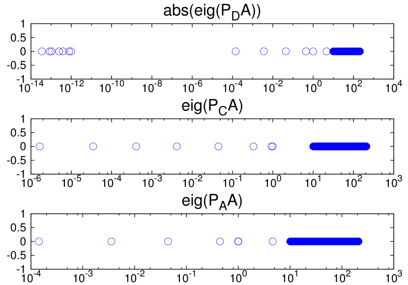
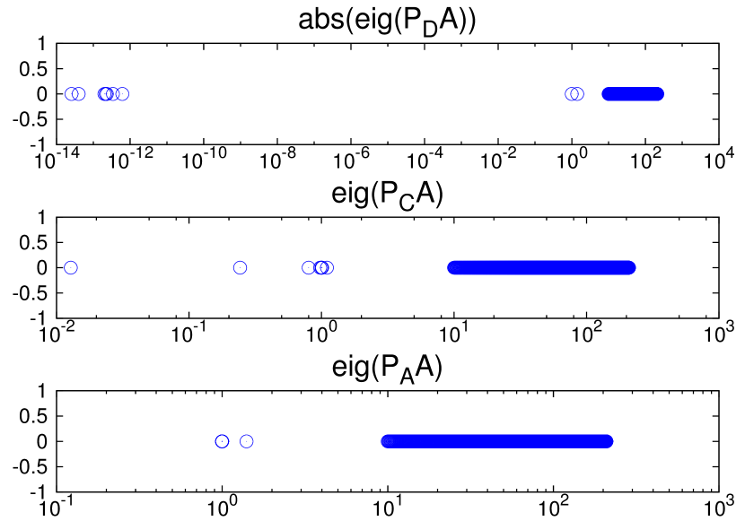
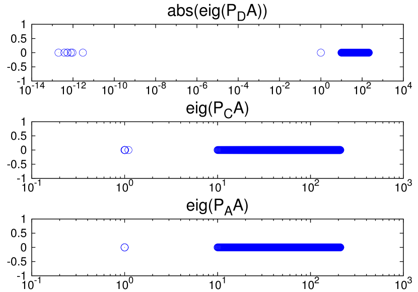
Figure 2 and Figure 2 show the eigenvalue distribution of the system preconditioned by the three preconditioners. As discussed in Section 2, because of rounding error, PDAsubscript𝑃𝐷𝐴P_{D}A has some tiny eigenvalues around zero. In general, it is difficult to figure out the condition under which these tiny eigenvalues cause the stagnation in the convergence. For the test case of diagonal matrix, rounding error does not impact the convergence of PDAsubscript𝑃𝐷𝐴P_{D}A when the perturbation in the coarse space is significantly small. We also see that the spectrum of PAAsubscript𝑃𝐴𝐴P_{A}A is more clustered than that of PCAsubscript𝑃𝐶𝐴P_{C}A, which is consistent with the estimated bounds of their spectrum described in Theorem 6 and Theorem 7.
Refer to caption
Fig. 1: The eigenvalue distribution of the preconditioned system. The preconditioners PDsubscript𝑃𝐷P_{D}, PCsubscript𝑃𝐶P_{C} and PAsubscript𝑃𝐴P_{A} are built with Z=V+rand/1e+03𝑍𝑉𝑟𝑎𝑛𝑑1𝑒03Z=V+rand/1e+03 and E1superscript𝐸1E^{-1}.
Refer to caption
Fig. 2: The eigenvalue distribution of the preconditioned system. The preconditioners PDsubscript𝑃𝐷P_{D}, PCsubscript𝑃𝐶P_{C} and PAsubscript𝑃𝐴P_{A} are built with Z=V+rand/1e+05𝑍𝑉𝑟𝑎𝑛𝑑1𝑒05Z=V+rand/1e+05 and E1superscript𝐸1E^{-1}.

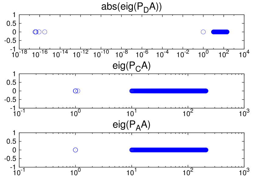
In Table 3, the first three rows show the number of GMRES iterations when only the projection matrix has perturbation. The difference of H~1superscript~𝐻1\tilde{H}^{-1} and E~1superscript~𝐸1\tilde{E}^{-1} is reported in the last two rows. In comparison with the second column in Table 2, we conclude the perturbation in the projection matrix has a little impact on PCsubscript𝑃𝐶P_{C} and PAsubscript𝑃𝐴P_{A}, but has a severe impact on PDsubscript𝑃𝐷P_{D} even when H~1superscript~𝐻1\tilde{H}^{-1} is very close to E~1superscript~𝐸1\tilde{E}^{-1} (see the last column).

Table 3: The number of GMRES iterations with different preconditioners, where only the projection matrix is perturbed and the perturbation of E~~𝐸\tilde{E} is H~=E~+rand/ε~𝐻~𝐸𝑟𝑎𝑛𝑑𝜀\tilde{H}=\tilde{E}+rand/\varepsilon.
ε=1e+10𝜀1𝑒10\varepsilon=1e+10 ε=1e+12𝜀1𝑒12\varepsilon=1e+12 ε=1e+14𝜀1𝑒14\varepsilon=1e+14 ε=1e+16𝜀1𝑒16\varepsilon=1e+16
PDsubscript𝑃𝐷P_{D} >>300 >>300 >>300 >>300
PCsubscript𝑃𝐶P_{C} 111 104 104 104
PAsubscript𝑃𝐴P_{A} 88 88 80 80
H~1E~I2subscriptnormsuperscript~𝐻1~𝐸𝐼2\|\tilde{H}^{-1}\tilde{E}-I\|_{2} 1.68e-03 1.08e-05 1.77e-07 1.23e-09
E~H~1I2subscriptnorm~𝐸superscript~𝐻1𝐼2\|\tilde{E}\tilde{H}^{-1}-I\|_{2} 1.68e-03 1.08e-05 1.77e-07 1.23e-09

Figure 4 and Figure 4 report the spectral distribution of PDsubscript𝑃𝐷P_{D}, PCsubscript𝑃𝐶P_{C} and PAsubscript𝑃𝐴P_{A}. We see that PCsubscript𝑃𝐶P_{C} and PAsubscript𝑃𝐴P_{A} successfully shift the small eigenvalues of A𝐴A to around one. Due to the perturbation in the projection matrix, PDsubscript𝑃𝐷P_{D} fails to deflate the small eigenvalues and thus yields some tiny eigenvalues around zero, which leads to a worse convergence (see the first row in Table 3).
Refer to caption
Fig. 3: The eigenvalue distribution of the preconditioned system, where the preconditioners PDsubscript𝑃𝐷P_{D}, PCsubscript𝑃𝐶P_{C} and PAsubscript𝑃𝐴P_{A} are built with V𝑉V and H~=E~+rand/1e+12~𝐻~𝐸𝑟𝑎𝑛𝑑1𝑒12\tilde{H}=\tilde{E}+rand/1e+12.
Refer to caption
Fig. 4: The eigenvalue distribution of the preconditioned system, where the preconditioners PDsubscript𝑃𝐷P_{D}, PCsubscript𝑃𝐶P_{C} and PAsubscript𝑃𝐴P_{A} are built with V𝑉V and H~=E~+rand/1e+16~𝐻~𝐸𝑟𝑎𝑛𝑑1𝑒16\tilde{H}=\tilde{E}+rand/1e+16.

4.2 Boundary value problem

We solve the following model problem

(κu)𝜅𝑢\displaystyle-\nabla\cdot(\kappa\nabla u) =\displaystyle= finΩ=[0,1]2,𝑓inΩsuperscript012\displaystyle f~{}~{}\mbox{in}~{}~{}\Omega=[0,1]^{2},
u𝑢\displaystyle u =\displaystyle= 0onΩ,0onΩ\displaystyle 0~{}~{}\mbox{on}~{}~{}\partial\Omega,

by the two-level multiplicative Schwarz method [8]. Here, κ𝜅\kappa is the diffusion function of x𝑥x and y𝑦y. The model problem is discretized by FreeFem++ [15] and the resulting coefficient matrix is of size 10201. Tests are performed on irregular overlapping decompositions with the overlap of 2 elements. These overlapping decompositions are built by adding the immediate neighboring vertices to non-overlapping subdomain obtained by Metis [9].

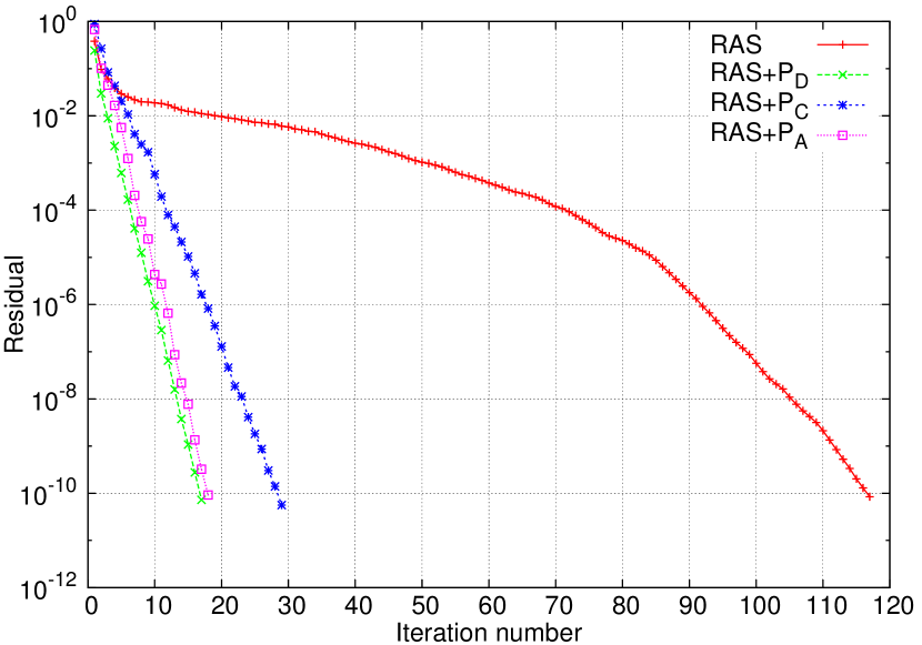
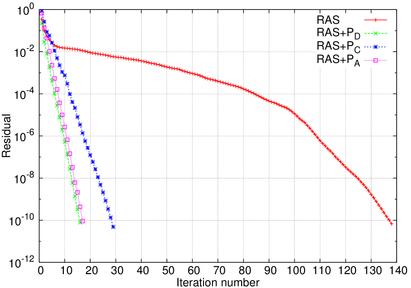
In the two-level multiplicative Schwarz method, the first level preconditioner is the restricted additive Schwarz preconditioner (RAS) [1] that is responsible to remove high frequency modes of the original system, and the deflation, coarse correction and adapted deflation preconditioners are applied as the second level preconditioners that remove lower frequency ones of the system preconditioned by one-level preconditioner [11, 8].

We choose Ritz vectors to span the coarse space, which are extracted from the Krylov subspace during the solve of the system preconditioned by RAS. These vectors are the approximate eigenvectors corresponding to the lower part of the spectrum of the preconditioned system. To enrich the information on lower part of the spectrum, we construct the coarse space by splitting Ritz-vectors, see [11, 8, 19] and references therein. More precisely, let

V=[v11v12v1,rv21v22v2,rvnparts,1vnparts,2vnparts,r]𝑉delimited-[]subscript𝑣11subscript𝑣12subscript𝑣1𝑟subscript𝑣21subscript𝑣22subscript𝑣2𝑟missing-subexpressionmissing-subexpressionmissing-subexpressionsubscript𝑣𝑛𝑝𝑎𝑟𝑡𝑠1subscript𝑣𝑛𝑝𝑎𝑟𝑡𝑠2subscript𝑣𝑛𝑝𝑎𝑟𝑡𝑠𝑟\displaystyle V=\left[\begin{array}[]{llll}v_{11}&v_{12}&\cdots&v_{1,r}\\ v_{21}&v_{22}&\cdots&v_{2,r}\\ \cdots&&&\\ v_{nparts,1}&v_{nparts,2}&\cdots&v_{nparts,r}\end{array}\right]

store Ritz vectors columnwise, where nparts𝑛𝑝𝑎𝑟𝑡𝑠nparts is the number of subdomains and r𝑟r the number of Ritz vectors; let Zisubscript𝑍𝑖Z_{i} store the orthogonal vectors obtained by orthogonalizing (vi1,vi2,,vi,r)subscript𝑣𝑖1subscript𝑣𝑖2subscript𝑣𝑖𝑟(v_{i1},v_{i2},\cdots,v_{i,r}). Then Z𝑍Z is formed as follows

Z=[Z1000Z2000Znparts].𝑍delimited-[]subscript𝑍1000subscript𝑍2000subscript𝑍𝑛𝑝𝑎𝑟𝑡𝑠\displaystyle Z=\left[\begin{array}[]{cccc}Z_{1}&0&\cdots&0\\ 0&Z_{2}&\cdots&0\\ \vdots&\vdots&\cdots&\vdots\\ 0&0&\cdots&Z_{nparts}\end{array}\right].

Obviously, span{V𝑉V} is a subspace of span{Z𝑍Z}; span{Z𝑍Z} is nparts𝑛𝑝𝑎𝑟𝑡𝑠nparts times as large as span{V𝑉V}. So span{Z𝑍Z} might have richer information corresponding to small eigenvalues.

Some comparisons of the three preconditioners are performed on two different configurations with highly heterogeneous coefficient κ𝜅\kappa. See [11] for details. Two cases are described as following:

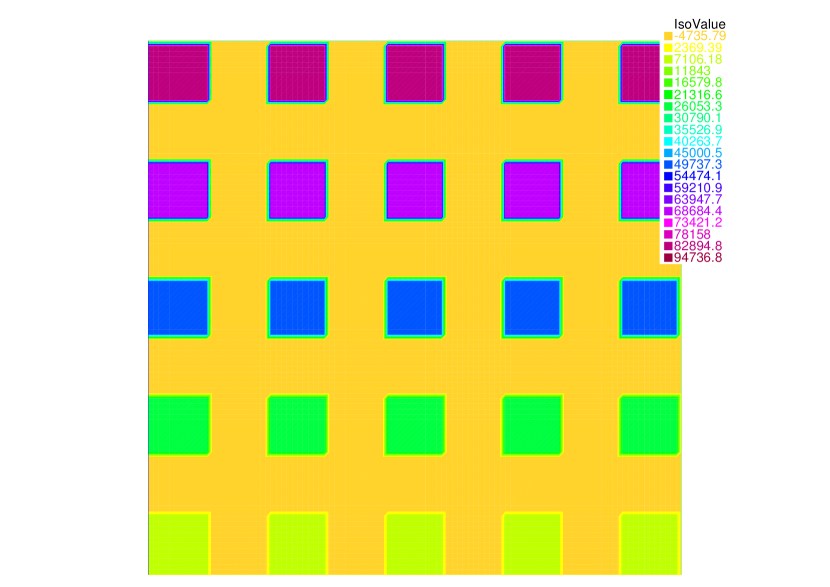
  • skyscraper κ𝜅\kappa: for x𝑥x and y𝑦y such that for [9x]\equiv0(mod 2) and [9y]\equiv0(mod 2), κ=104([9y]+1)𝜅superscript104delimited-[]9𝑦1\kappa=10^{4}([9y]+1); and κ=1𝜅1\kappa=1 elsewhere. See Figure 6.

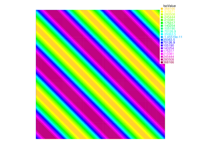
  • continuous κ𝜅\kappa: κ(x,y)=106/3sin(4π(x+y)+0.1)𝜅𝑥𝑦superscript10634𝜋𝑥𝑦0.1\kappa(x,y)=10^{6}/3\sin(4\pi(x+y)+0.1). See Figure 6.

For both cases, we use the zero vector as the initial guess vector. The iteration will stop when the relative residual is less than 1010superscript101010^{-10}. Moreover, we construct the coarse space with all the eigenvectors associated with the eigenvalues less than 0.5 against the various domain decompositions.
Refer to caption
Fig. 5: Skyscraper case
Refer to caption
Fig. 6: Continuous case

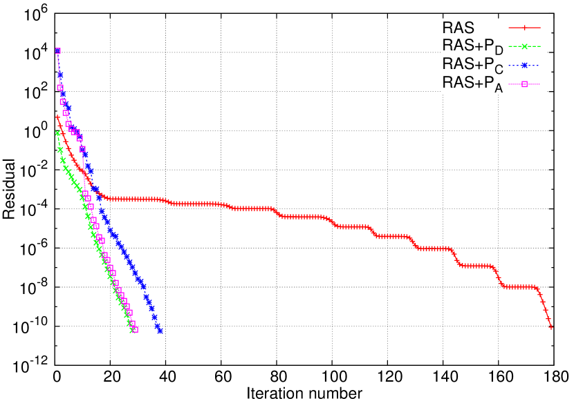
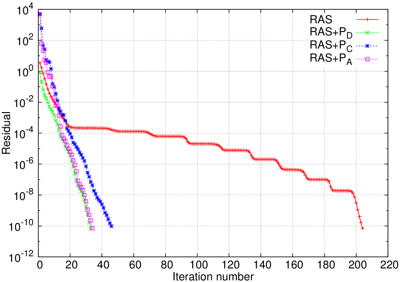
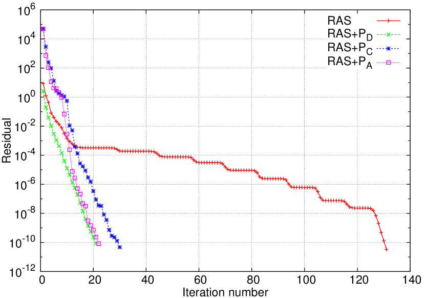
In Figures 8-10, we report the convergence curves for the skycraper case against the various number of subdomains. Compared to one-level method, all three two-level methods improve convergence sufficiently. PDsubscript𝑃𝐷P_{D} and PAsubscript𝑃𝐴P_{A} have almost the same number of iterations although the initial residual of PDsubscript𝑃𝐷P_{D} is much less than that of PAsubscript𝑃𝐴P_{A}. PDsubscript𝑃𝐷P_{D} and PAsubscript𝑃𝐴P_{A} are more efficient than PCsubscript𝑃𝐶P_{C}. Two-level method varies slightly on the number of iterations as the number of subdomains increases, while one-level method does.
Refer to caption
Fig. 7: Skyscraper case with 16 subdomains. 16 Ritz vectors spanning the coarse space.
Refer to caption
Fig. 8: Skyscraper case with 32 subdomains. 16 Ritz vectors spanning the coarse space.
Refer to caption
Fig. 9: Skyscraper case with 64 subdomains. 16 Ritz vectors spanning the coarse space.
Refer to caption
Fig. 10: Skyscraper case with 128 subdomains. 16 Ritz vectors spanning the coarse space.

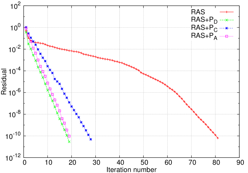
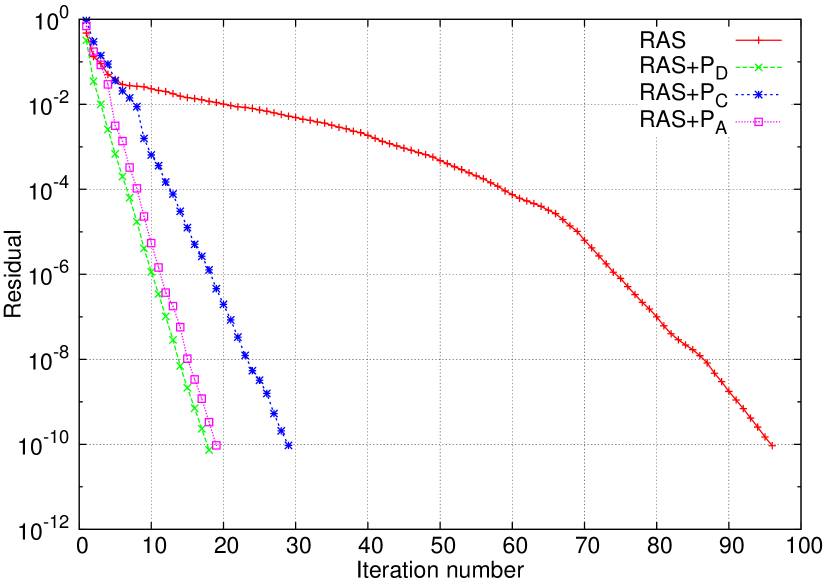
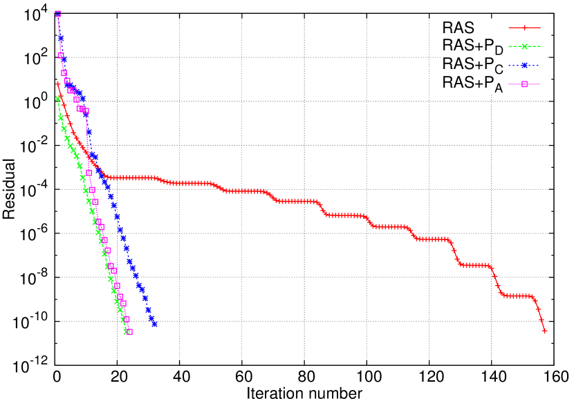
Figures 12-14 plot the convergence curves for the continuous case against the various number of subdomains. Once again, we see that two-level method with RAS and the three preconditioners all outperform one-level method with only RAS. Like the skycraper case, PDsubscript𝑃𝐷P_{D} and PAsubscript𝑃𝐴P_{A} have almost the same number of iterations for all four decompositions and outperform PCsubscript𝑃𝐶P_{C}.

Refer to caption
Fig. 11: Continuous case with 16 subdomains. 15 Ritz vectors spanning the coarse space.
Refer to caption
Fig. 12: Continuous case with 32 subdomains. 15 Ritz vectors spanning the coarse space.
Refer to caption
Fig. 13: Continuous case with 64 subdomains. 16 Ritz vectors spanning the coarse space.
Refer to caption
Fig. 14: Continuous case with 128 subdomains. 15 Ritz vectors spanning the coarse space.

In Table 4, we report the maximal residual of Ritz pairs for both cases that are extracted from the Krylov subspace when solving the system preconditioned only by RAS.

Table 4: Maximal residual of Ritz pairs for the skyscraper and continuous cases.
Nparts 16 32 64 128
skyscraper 2.564719e-09 9.162259e-08 1.577898e-08 4.747077e-09
continuous 4.439121e-03 5.242112e-03 4.749042e-03 1.326165e-03

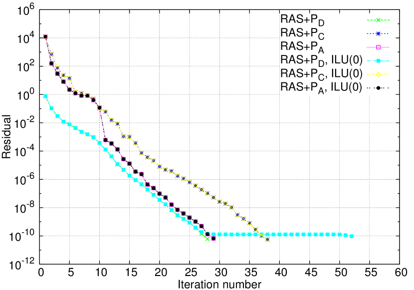
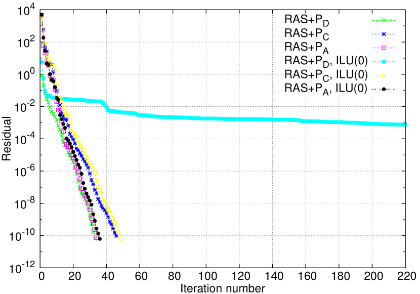
Note that the projection matrix E𝐸E is large in the case that the decomposition has 64 or 128 subdomains. As a consequence, computing LU factorization of E1superscript𝐸1E^{-1} is costly and impairs the gains in the number of iterations. Hence, we attempt to compute the incomplete LU factorization of E𝐸E, which is cheaper to compute than the LU factorization. Assume L𝐿L and U𝑈U are factors of an incomplete LU factorization with no fill-in (ILU(0)) of E𝐸E. Note that E𝐸E has a sparse structure because of the sparse structure of Z𝑍Z. So L𝐿L and U𝑈U are sparse as well. This means that it is very cheap to solve (LU)x=y𝐿𝑈𝑥𝑦(LU)x=y. In this way, E𝐸E is actually replaced by LU𝐿𝑈LU.

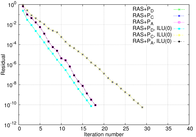
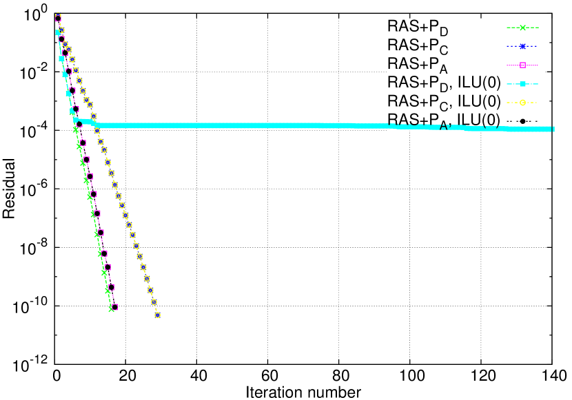
From Figure 16 and Figure 16, it appears that the perturbation in E𝐸E has almost no impact on PAsubscript𝑃𝐴P_{A} and PCsubscript𝑃𝐶P_{C} for the skycraper case, but has severe impact on PDsubscript𝑃𝐷P_{D} that leads to a stagnation in the convergence. Figure 18 and Figure 18 show that PAsubscript𝑃𝐴P_{A} and PCsubscript𝑃𝐶P_{C} are also stable for the continuous case. As is shown in Figure 18, PDsubscript𝑃𝐷P_{D} is still unstable when the perturbation in E𝐸E is not small enough (see the second column in Table 6). However, Figure 18 shows that PDsubscript𝑃𝐷P_{D} is stable, since the perturbation is small enough such that LU𝐿𝑈LU is almost same as E𝐸E (see the first column in Table 6).

Table 5 and Table 6 present the distance between LU𝐿𝑈LU and E𝐸E for both cases, respectively.

Refer to caption
Fig. 15: Skyscraper case with 64 subdomains. E𝐸E is replaced by LU𝐿𝑈LU.
Refer to caption
Fig. 16: Skyscraper case with 128 subdomains. E𝐸E is replaced by LU𝐿𝑈LU.
Table 5: The distance between LU𝐿𝑈LU and E𝐸E for the skyscraper case.
Nparts 64 128
E(LU)1I2subscriptnorm𝐸superscript𝐿𝑈1𝐼2\|E(LU)^{-1}-I\|_{2} 3.8588e-08 8.9712e+02
(LU)1EI2subscriptnormsuperscript𝐿𝑈1𝐸𝐼2\|(LU)^{-1}E-I\|_{2} 4.1433e-10 8.6292
Refer to caption
Fig. 17: Continuous case with 64 subdomains. E𝐸E is replaced by LU𝐿𝑈LU.
Refer to caption
Fig. 18: Continuous case with 128 subdomains. E𝐸E is replaced by LU𝐿𝑈LU.
Table 6: The distance between LU𝐿𝑈LU and E𝐸E for the continuous case.
Nparts 64 128
E(LU)1I2subscriptnorm𝐸superscript𝐿𝑈1𝐼2\|E(LU)^{-1}-I\|_{2} 4.1008e-14 5.4090e-01
(LU)1EI2subscriptnormsuperscript𝐿𝑈1𝐸𝐼2\|(LU)^{-1}E-I\|_{2} 1.3890e-15 1.0215e-01

5 Conclusion

We presented a perturbation analysis on the deflation, coarse correction and adapted deflation preconditioners when the inexact coarse space and inverse of projection matrix are applied for the construction of the preconditioners. Our analysis shows that in exact arithmetic the spectrum of the system preconditioned by the three preconditioners is impacted by the angle between the exact coarse space and the perturbed one. Moreover, we prove that the coarse correction and adapted deflation preconditioners are insensitive to the perturbation of the projection matrix, whereas the deflation preconditioner is sensitive. Numerical results of the different test cases confirm the perturbation analysis.

Acknowledgements. The author would like to appreciate Professor Xiao-Chuan Cai for his valuable comments that are very helpful to improve the presentation of this paper.

References

  • [1] X.-C. Cai and M. Sarkis, A restricted additive Schwarz preconditioner for general sparse linear systems, SIAM J. Sci. Comput., 21 (1999), pp. 792-797.
  • [2] Y. A. Erlangga and R. Nabben, Multilevel projection-based nested Krylov iteration for boundary value problems, SIAM J. Sci. Comput., 30 (2008), pp. 1572-1595.
  • [3] Y. A. Erlangga and R. Nabben, Deflation and balancing preconditioners for Krylov subspace methods applied to nonsymmetric matrices, SIAM J. Matrix Anal. Appl., 30 (2008), pp. 684-699.
  • [4] E. Efstathiou and M. J. Gander, Why restricted additive Schwarz converges faster than additive Schwarz, BIT Numerical Mathematics, 43 (2003), pp. 945-959.
  • [5] L. Giraud and S. Gratton, On the sensitivity of some spectral preconditioners, SIAM J. Matrix Anal. Appl., 27 (2006), pp. 1089-1105.
  • [6] G. H. Golub and C. F. Van Loan, Matrix Computations, 3rd Edition, John Hopkins University Press, Baltimore, MD, 1996.
  • [7] P. Gosselet and C. Rey, On a selective reuse of Krylov subspaces in Newton-Krylov approaches for nonlinear elasticity, In Domain decomposition methods in science and engineering, pages 419-426(electronic). Natl. Auton. Univ. Mex., México, 2003.
  • [8] P. Havé, R. Masson, F. Nataf, M. Szydlarski, H. Xiang, and T. Zhao, Algebraic domain decomposition methods for highly heterogeneous problems, to appear in SIAM J. Sci. Comput., 2013.
  • [9] G. Karypis and V. Kumar, A fast and highly qualty multilevel scheme for partitioning irregular graphs, SIAM J. Sci. Comput., 20 (1998), pp. 359-392.
  • [10] R. B. Morgan, GMRES with deflated restarting, SIAM J. Sci. Comput., 24 (2002), pp. 20-37.
  • [11] F. Nataf, H. Xiang, V. Dolean, and N. Spillane, A coarse grid space construction based on local Dirichlet to Neumann maps, SIAM J. Sci. Comput., 33 (2011), pp. 1623-1642.
  • [12] R. Nabben and C. Vuik, A comparison of deflation and the balancing preconditioner, SIAM J. Sci. Comput., 27 (2006), pp. 1742-1759.
  • [13] A. Padiy, O. Axelsson, and B. Polman, Generalized augmented matrix preconditioning approach and its application to iterative solution of ill-conditioned algebraic systems, SIAM J. Matrix Anal. Appl., 22 (2000), pp. 793-818.
  • [14] M. L. Parks, E. de Sturler, G. Mackey, D. D. Johnson, and S. Maiti, Recycling Krylov subspaces for sequences of linear systems, SIAM J. Sci. Comput., 28 (2006), pp. 1651-1674.
  • [15] O. Pironneau, F. Hecht, A. Le Hyric, and J. Morice, FreeFem++, Laboratoire J.-L. Lions, Université Pierre et Marie Curie, available online at http://www.freefem.org/ff++/, 3.7 edition, 2010.
  • [16] Y. Saad, Iterative Methods for Sparse Linear Systems, SIAM, 2003.
  • [17] A. ST-CYR, M. J. Gander, and S. J. Thomas, Optimized multiplicative, additive, and restricted additive Schwarz preconditioning, SIAM J. Sci. Comput., 29 (2007), pp. 2402-2425.
  • [18] G. W. Stewart, Matrix Algorithms Volume II: Eigensystems, SIAM, 2001.
  • [19] J. M. Tang, R. Nabben, C. Vuik, and Y. A. Erlangga, Comparison of two-level preconditioners derived from deflation, domain decomposition and multigrid methods, J.Sci.Comput., 39 (2009), pp. 340-370.