Thermal entanglement in an orthogonal dimer-plaquette chain with alternating Ising-Heisenberg coupling

Abstract

In this paper we explore the entanglement in orthogonal dimer-plaquette Ising-Heisenberg chain, assembled between plaquette edges, also known as orthogonal dimer plaquettes. The quantum entanglement properties involving an infinite chain structure are quite important, not only because the mathematical calculation is cumbersome but also because real materials are well represented by infinite chain. Using the local gauge symmetry of this model, we are able to map onto a simple spin-1 like Ising and spin-1/2 Heisenberg dimer model with single effective ion anisotropy. Thereafter this model can be solved using the decoration transformation and transfer matrix approach. First, we discuss the phase diagram at zero temperature of this model, where we find five ground states, one ferromagnetic, one antiferromagnetic, one triplet-triplet disordered and one triplet-singlet disordered phase, beside a dimer ferromagnetic-antiferromagnetic phase. In addition, we discuss the thermodynamic properties such as entropy, where we display the residual entropy. Furthermore, using the nearest site correlation function it is possible also to analyze the pairwise thermal entanglement for both orthogonal dimers, additionally we discuss the threshold temperature of the entangled region as a function of Hamiltonian parameters. We find quite interesting thin reentrance threshold temperature for one of the dimers, and we also discuss the differences and similarities for both dimers.

I Introduction

Recently, several theoretical investigation are dedicated to quantum entanglement, which is one of the most fascinating types of correlations that can be shared only among quantum systemsAmicoHorod . In recent years, many efforts have been devoted to characterizing qualitatively and quantitatively the entanglement properties of condensed matter systems, which are the natural candidate for application in quantum communication and quantum information. In this sense, it is quite relevant to study the entanglement of solid state systems such as spin chainsqubit-Heisnb . The Heisenberg chain is one of the simplest quantum systems, which exhibits the entanglement, due to the Heisenberg interaction is non localized in the spin system. Several studies have been done on the threshold temperature for the pairwise thermal entanglement in the Heisenberg model with a finite number of qubits. Thermal entanglement of the isotropic Heisenberg chain has been studied in the absence wang and in the presence of external magnetic field arnesen .

On the other hand, quasi two-dimensional magnets have been attracted since 90 decades, such as the quasi-two-dimensional magnet $\mathrm{CaV}_{4}\mathrm{O}_{9}$tanigushi , that has a layered structure where the magnetic $\mathrm{V}^{4+}$ ions have spin 1/2 and form a 1/5-depleted square lattice. As well as the polycrystalline $\text{SrCu}_{2}\text{(BO}_{3})_{2}$ having a two dimensional (2D) orthogonal network of Cu dimers, this cuprate, provides a 2D spin-gap system in which the ground state can be solved exactlymiyahara ; kageyama . These quasi-two-dimensional systems are topologically equivalent to the theoretical model proposed by Shastry and Sutherlandshastry .

Motivated by the above real materials Ivanov and Richterivanov proposed the class of one-dimensional Heisenberg spin models (plaquette chains) related to the real materialstanigushi ; miyahara ; kageyama , were analyzed the zero temperature magnetic properties through numerical and analytical results ivanov ; richter . While in reference schu was discussed the sequence of first-order quantum phase transitions in a frustrated spin half dimer-plaquette chain. A detailed investigation about the first-order quantum phase transition of the orthogonal-dimer spin chain also was considered by Koga et al.koga , as well as the frustration-induced phase transitions in the spin-$S$ orthogonal-dimer chainkoga02 .

A more recent investigation was developed by Ohanyan and Honeckervadim12 , where they have been discussed the magnetothermal properties of the Ising-Heisenberg orthogonal-dimer chain with triangular XXZ clusters. Furthermore, in the last decade several quasi-one-dimensional Ising-Heisenberg model such as diamond chain were intensively investigated, mainly the thermodynamic properties and geometric frustrationstrecka06 ; strecka09 ; valverde ; vadim , magneto-caloric effectpereira2 , as well as thermal entanglementspra ; entg-ananik , among other physical quantities. Some other variant of the Ising-Heisenberg model also were considered, such as Ising-Hubbard modellisnii and Hubbard model in the quasi-atomic limithubbard besides spinless electronsspinless in diamond chain.

The outline of this work is as follows. In sec. 2 we present the dimer-plaquette Ising-Heisenberg chain; it is also discussed the zero temperature phase diagram. In sec. 3 we present the exact thermodynamic solution of the model, thus we discuss the entropy, specific heat and correlation function. In sec. 4 we discuss the thermal entanglement and its threshold temperature. Finally in sec. 5, we summarize our results and draw our conclusions.

II Orthogonal dimer-plaquette Ising-Heisenberg chain

Figure 1: (Color online) Schematic representation of dimer-plaquette Ising-Heisenberg chain. (Above) Thick line correspond to Heisenberg coupling, while the thin line corresponds to Ising coupling. (Below) Dimer plaquette mapping through local gauge symmetry.

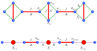
The theoretical investigation of the orthogonal dimer-plaquette models are motivated not only from the theoretical point of view, but also from the experimental viewpoint. It is worth to remark that the Heisenberg orthogonal dimer-plaquette model cannot be solved exactly at finite temperature. Driven by the comments given in the introduction, we consider the orthogonal-dimer plaquette chain with Ising-Heisenberg coupling as schematically described in figure 1. Therefore, the Hamiltonian for an orthogonal dimer-plaquette chain could be expressed by

$$H= -\sum_{i=1}^{N}\left\{J^{\prime}(\boldsymbol{\sigma}_{a,i},\boldsymbol{\sigma}_{b,i})_{\Delta^{\prime}}+J(\boldsymbol{\sigma}_{c,i},\boldsymbol{\sigma}_{d,i})_{\Delta}\right.$$

$$\left.+J_{0}[(\sigma_{a,i}^{z}+\sigma_{b,i}^{z})\sigma_{c,i}^{z}+(\sigma_{a,i+1}^{z}+\sigma_{b,i+1}^{z})\sigma_{d,i}^{z}]\right\},$$ (1)

with

$$J^{\prime}(\boldsymbol{\sigma}_{a,i},\boldsymbol{\sigma}_{b,i})_{\Delta^{\prime}}=J^{\prime}(\sigma_{a,i}^{x}\sigma_{b,i}^{x}+\sigma_{a,i}^{y}\sigma_{b,i}^{y})+\Delta^{\prime}\sigma_{a,i}^{z}\sigma_{b,i}^{z}$$ (2)

where $\sigma_{\gamma,i}^{\alpha}$ are the spin operators also known as Pauli matrices (with $\alpha=\{x,y,z\}$) at plaquette $i$ for particles $\gamma=\{a,b,c,d\}$, for detail see figure 1. The thick line correspond to Heisenberg coupling, while the thin line corresponds to Ising coupling. The Ising coupling parameter is denoted by $J_{0}$, whereas $J$ ($J^{\prime}$) represents the $x$ and $y$ components of Heisenberg coupling and with $\Delta$ ($\Delta^{\prime}$) we mean the anisotropic ($z$-component) coupling in the Heisenberg term for $ab$-dimer and $cd$-dimer respectively.

To transform this model onto the well known mixed spin "Ising"–Heisenberg model, we use the following definition $S_{i}^{\alpha}=\sigma_{a,i}^{\alpha}+\sigma_{b,i}^{\alpha}$. By the use of $S_{i}^{\alpha}$ definition we obtain the identity: $(S_{i}^{\alpha})^{2}=2+2\sigma_{a,i}^{\alpha}\sigma_{b,i}^{\alpha}$. Thereafter, we can easily establish the following transformation

$$J^{\prime}(\boldsymbol{\sigma}_{a,i},\boldsymbol{\sigma}_{b,i})_{\Delta^{\prime}}=\frac{J^{\prime}}{2}\boldsymbol{S}_{i}^{2}+\frac{\Delta^{\prime}-J^{\prime}}{2}\left(S_{i}^{z}\right)^{2}-(2J^{\prime}+\Delta^{\prime}),$$ (3)

and by $\boldsymbol{S}_{i}^{2}$ we just denote $\boldsymbol{S}_{i}^{2}=\boldsymbol{S}_{i}.\boldsymbol{S}_{i}$, so, this matrix is given by

$$\boldsymbol{S}_{i}^{2}=4\left[\begin{array}[]{cccc}2&0&0&0\\ 0&1&1&0\\ 0&1&1&0\\ 0&0&0&2\end{array}\right],$$ (4)

rewritten the Hamiltonian in terms of operators $S_{i}^{z}$ and $\boldsymbol{S}_{i}^{2}$ we have an Ising-Heisenberg chain model whose Hamiltonian is given by $H=H_{0}+H^{\prime}$, with $H_{0}=(2J^{\prime}+\Delta^{\prime})N$. Therefore, the transformed Hamiltonian reduce to

$$H^{\prime}= -\sum_{i=1}^{N}\left\{\tfrac{J^{\prime}}{4}(\boldsymbol{S}_{i}^{2}+\boldsymbol{S}_{i+1}^{2})+\tfrac{\Delta^{\prime}-J^{\prime}}{4}\left[\left(S_{i}^{z}\right)^{2}+\left(S_{i+1}^{z}\right)^{2}\right]\right.$$

$$\left.+J(\boldsymbol{\sigma}_{c,i},\boldsymbol{\sigma}_{d,i})_{\Delta}+J_{0}\left(S_{i}^{z}\sigma_{c,i}^{z}+\sigma_{d,i}^{z}S_{i+1}^{z}\right)\right\}.$$ (5)

We can observe from eq.(4) the matrix has a $2\times 2$ block matrix; hence, we can diagonalize this block matrix. It is interesting to note that the matrix $S_{i}^{z}$ is still diagonal in the new basis, due to corresponding $2\times 2$ block matrix be null. Then, this means we can simultaneously diagonalize both matrices $S_{i}^{z}$ and $\boldsymbol{S}_{i}^{2}$. Recall those $S_{i}^{z}$ and $\boldsymbol{S}_{i}^{2}$ are commutative operators. So, the diagonal matrices are expressed by

$$\boldsymbol{S}_{i}^{2}=\left[\begin{array}[]{cccc}8&0&0&0\\ 0&8&0&0\\ 0&0&0&0\\ 0&0&0&8\end{array}\right]\quad\text{and}\quad S_{i}^{z}=\left[\begin{array}[]{cccc}2&0&0&0\\ 0&0&0&0\\ 0&0&0&0\\ 0&0&0&-2\end{array}\right],$$ (6)

and whose corresponding eigenvector states are expressed as

$$|\tau_{+1}\rangle= |\begin{smallmatrix}+\\ +\end{smallmatrix}\rangle,$$ (7)

$$|\tau_{0}\rangle= \frac{1}{\sqrt{2}}\left(|\begin{smallmatrix}+\\ -\end{smallmatrix}\rangle+|\begin{smallmatrix}-\\ +\end{smallmatrix}\rangle\right),$$ (8)

$$|s_{0}\rangle= \frac{1}{\sqrt{2}}\left(|\begin{smallmatrix}+\\ -\end{smallmatrix}\rangle-|\begin{smallmatrix}-\\ +\end{smallmatrix}\rangle\right),$$ (9)

$$|\tau_{-1}\rangle= |\begin{smallmatrix}-\\ -\end{smallmatrix}\rangle.$$ (10)

The effective Ising "spin" in Hamiltonian (5) can be understood as a composition of one triplet state and one singlet state.

This transformation is possible because, the local gauge symmetry is only satisfied by Hamiltonian (1) when the Ising couplings $ac$ ($ad$) and $bc$($bd$) are identical.

II.1 The zero temperature phase diagram

In order to analyze the phase diagram of the orthogonal-dimer plaquette, we assume the particular case $J^{\prime}=J$ and $\Delta^{\prime}=\Delta$, following the parameter used in the literaturekoga ; koga02 ; schu .

The dimer-plaquette Ising-Heisenberg chain described by the Hamiltonian (1) exhibit five ground states. These states are expressed as

$$|FM\rangle= \prod_{i=1}^{N}|\begin{smallmatrix}+\\ +\end{smallmatrix}\rangle_{i}\otimes|++\rangle_{i},$$ (11)

$$|AFM\rangle= \prod_{i=1}^{N}|\begin{smallmatrix}+\\ +\end{smallmatrix}\rangle_{i}\otimes|--\rangle_{i},$$ (12)

For the ferromagnetic (FM) phase and antiferromagnetic (AFM) phase the corresponding eigenvalues are given by

$$E_{FM}= -2J^{\prime}-2\Delta^{\prime}-\Delta-4J_{0},$$

$$E_{AFM}= -2J^{\prime}-2\Delta^{\prime}-\Delta+4J_{0}.$$

The other phase are composed by dimers in triplet-triplet (TT) phase and triplet-singlet (TS) phase,

$$|TT\rangle= \prod_{i=1}^{N}|\tau_{0}\rangle_{i}\otimes\frac{1}{\sqrt{2}}\left(|+-\rangle_{i}+|-+\rangle_{i}\right),$$ (13)

$$|TS\rangle= \prod_{i=1}^{N}|\tau_{0}\rangle_{i}\otimes\frac{1}{\sqrt{2}}\left(|+-\rangle_{i}-|-+\rangle_{i}\right),$$ (14)

where the corresponding eigenvalues become

$$E_{TT}= \Delta-2J-4J^{\prime},$$

$$E_{TS}= \Delta+2{\it J}.$$

It is worthy to mention that the state given by eqs.(13) and (14) becomes frustrated state only when $J=0$ (Ising limit).

Finally, the dimer-antiferromagnetic (DFA) state can be expressed by

$$|DFA\rangle= \prod_{i=1}^{N/2}|\begin{smallmatrix}+\\ +\end{smallmatrix}\rangle_{i}\otimes|\eta_{2,-2}\rangle_{i}\otimes|\begin{smallmatrix}-\\ -\end{smallmatrix}\rangle_{i}\otimes|\eta_{2,-2}\rangle,$$ (15)

with

$$|\eta_{2,-2}\rangle=\frac{\left(|+-\rangle_{i}+\vartheta|-+\rangle_{i}\right)}{\sqrt{1+\vartheta^{2}}},$$ (16)

and

$$\vartheta=\frac{\sqrt{4J_{0}^{2}+J^{2}}+2J_{0}}{J}.$$ (17)

Hereafter the corresponding dimer-antiferromagnetic eigenvalue becomes

$$E_{DFA}= -2J^{\prime}-2\Delta^{\prime}+\Delta-2\sqrt{4J_{0}^{2}+J^{2}}.$$

Figure 2: (a) Phase diagram at zero temperature as a dependency of $J$ and $\Delta$ for a fixed value of $J_{0}=1$. (b) Phase diagram at zero temperature as a dependency of $J_{0}$ and $\Delta$ for a fixed value of $J=1$.

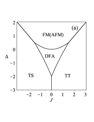
In order to display the phase diagram at zero temperature, we plot $J$ versus $\Delta$, assuming fixed value for $J_{0}=1(-1)$ FM(AFM) respectively. As shown in figure 2(a). For $\Delta<-2$, there is a boundary between TS and TT state at $J=0$, whereas for $-2\leqslant\Delta\leqslant 0.5$ the state TS (TT) is limited by DFA region whose boundary is given by $\Delta=2|J|-\sqrt{4+J^{2}}$, when $J>0$ ($J<0$) respectively. While for $\Delta\geqslant 0.5$ the state TS (TT) is limited by FM(AFM) region $\Delta=|J|-1$. Furthermore, the boundary between DFA and FM(AFM) region is represented by the curve $\Delta=\sqrt{4+J^{2}}-2$.

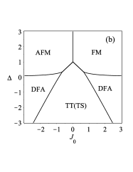
While in figure 2(b), we observe the phase diagram from another viewpoint, $\Delta$ against $J_{0}$, assuming fixed $J=1$. In this picture the TS and TT phase is displayed in same region, while AFM and FM states are illustrated for $J_{0}>0$ ($J_{0}<0$) respectively. The boundary between FM(AFM) and TT(TS) is given by $\Delta=1-|J_{0}|$ when $|J_{0}|<2/3$. Whereas the DFA region appears when $|J_{0}|>2/3$, which is limited by TT(TS) region and this boundary curve becomes $\Delta=2-\sqrt{4J_{0}^{2}+1}$, and finally the boundary between FM and AFM regions is described by the curve $\Delta=\sqrt{4J_{0}^{2}+1}-2|J_{0}|$.

III The thermodynamics of the model

The method to be used will be the decoration transformation proposed in early 50 decade by Syozi Syozi and Fisher Fisher . Afterward this approach was the subject of study in reference phys-A-09 , for the case of multi-spins. Similar generalization was developed by Strečka strecka pla for the hybrid system (e.g. Ising-Heisenberg). Another interesting variant of this approach also was discussed previously in reference JPA-11 , where a direct transformation was proposed instead of several step by step transformation. Consequently, the decoration transformation approach is widely used to solve spins models, besides, the decoration transformation approach can also be applied to electron coupling system such has been applied for the case of spinless fermion on diamond structurespinless , and as well as for Hubbard model in the quasi-atomic limithubbard .

In order to study the thermodynamics of the dimer-plaquette Ising-Heisenberg chain, we will use the decoration transformation proposed in reference JPA-11 together with the usual transfer matrix technique baxter-book . So, let us start considering the partition function as follow

$$\mathcal{Z}_{N}=\mathrm{e}^{-\beta H_{0}}\mathrm{tr}\left(\prod_{i=1}^{N}\mathrm{e}^{-\beta H^{\prime}}\right),$$ (18)

where $\beta=1/kT$, with $k$ being the Boltzmann constant and $T$ is the absolute temperature, and assuming $H^{\prime}$ is given by eq.(5).

The effective model can be solved by the usual transfer matrix approachbaxter-book . Inasmuch as the transfer matrix of the Hamiltonian (5) is reduced to

$$\boldsymbol{T}=\left[\begin{array}[]{cccc}w_{1,1}&w_{1,0}{x^{\prime}}^{2}&w_{1,0}&w_{1,-1}\\ w_{1,0}{x^{\prime}}^{2}&w_{0,0}{x^{\prime}}^{4}&w_{0,0}{x^{\prime}}^{2}&w_{1,0}{x^{\prime}}^{2}\\ w_{1,0}&w_{0,0}{x^{\prime}}^{2}&w_{0,0}&w_{1,0}\\ w_{1,-1}&w_{1,0}{x^{\prime}}^{2}&w_{1,0}&w_{1,1}\end{array}\right],$$ (19)

with

$$w_{1,1}= {x^{\prime}}^{2}{z^{\prime}}^{2}\left[z\left(y^{4}+y^{-4}\right)+z^{-1}(x^{2}+x^{-2})\right],$$ (20)

$$w_{1,0}= {x^{\prime}}{z^{\prime}}\left[z\left(y^{2}+y^{-2}\right)+z^{-1}(x_{1}^{2}+x_{1}^{-2})\right],$$ (21)

$$w_{1,-1}= {x^{\prime}}^{2}{z^{\prime}}^{2}\left[2z+z^{-1}\left(x_{2}^{2}+x_{2}^{-2}\right)\right],$$ (22)

$$w_{0,0}= 2z+z^{-1}\left(x^{2}+x^{-2}\right),$$ (23)

where we have introduced the following notations $x=\mathrm{e}^{\beta J}$ , $z=\mathrm{e}^{\beta\Delta}$, ${x^{\prime}}=\mathrm{e}^{\beta J^{\prime}}$ , ${z^{\prime}}=\mathrm{e}^{\beta\Delta^{\prime}}$ and $y=\mathrm{e}^{\beta J_{0}}$. Furthermore, we define also the following exponentials $x_{1}=\mathrm{e}^{\beta\sqrt{J^{2}+J_{0}^{2}}}$ and $x_{2}=\mathrm{e}^{\beta\sqrt{J^{2}+4J_{0}^{2}}}$.

In order to diagonalize the transfer matrix $\boldsymbol{T}$, we perform the determinant of the transfer matrix, which is expressed as follow

$$\lambda(\lambda^{2}-a_{1}\lambda+a_{0})(\lambda-w_{1,1}+w_{1,-1})=0,$$ (24)

here, the coefficients of the quadratic term eq.(24) is given by

$$a_{1}= w_{1,1}+w_{0,0}(1+{x^{\prime}}^{4})+w_{1,-1},$$ (25)

$$a_{0}= \left(1+{x^{\prime}}^{4}\right)\left[w_{0,0}\left(w_{1,1}+w_{1,-1}\right)-2w_{1,0}^{2}\right],$$

Therefore, the eigenvalues can be expressed as

$$\lambda_{0}= \tfrac{1}{2}\left(a_{1}+\sqrt{a_{1}^{2}-4a_{0}}\right),$$ (26)

$$\lambda_{1}= \tfrac{1}{2}\left(a_{1}-\sqrt{a_{1}^{2}-4a_{0}}\right),$$ (27)

$$\lambda_{2}= {x^{\prime}}^{2}{z^{\prime}}^{2}\left[z\left(y^{2}-y^{-2}\right)^{2}+\frac{\left(x^{2}+x^{-2}-x_{2}^{2}-x_{2}^{-2}\right)}{z}\right],$$ (28)

$$\lambda_{3}= 0.$$ (29)

In the thermodynamic limit, the free energy per unit cell is given only by the largest eigenvalue of transfer matrix, and for our case, we can easily verify the first eigenvalues $\lambda_{0}$ become always the largest one. Thus, the free energy can be expressed by the relation below

$$f=2J^{\prime}+\Delta^{\prime}-\frac{1}{\beta}\ln\left(\lambda_{0}\right).$$ (30)

The first term of the free energy is a trivial constant energy, obtained during the local gauge transformation, which is irrelevant for thermodynamis quantities. Note that the free energy is valid for arbitrary value of $J^{\prime}$ and $\Delta^{\prime}$, although here we consider only a particular case $J^{\prime}=J$ and $\Delta^{\prime}=\Delta$, following the parameter used in the literaturekoga ; koga02 ; schu . Therefore, any additional properties can be obtained straightforwardly from eq.(30).

III.1 Entropy and specific heat

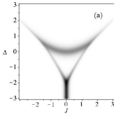
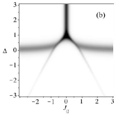
In order to accomplish with our discussion concerning to the thermodynamics properties. Let us illustrate the entropy ($\mathcal{S}=-\partial f/\partial T$) in fig. 3(a) for the low temperature limit as a function of $\Delta$ and $J$, whereas, in fig.3(b) the entropy is illustrated as a function of $\Delta$ and $J_{0}$. Dark region corresponds to higher entropy, while the white region corresponds to zero entropy. However, as soon as the temperature decreases the entropy leads to zero, unless, for $J=0$ and $\Delta\leqslant-2$ (pure Ising chain) the dark line will remain when temperature decreases, leading to a residual entropy $\mathcal{S}_{0}=2\ln(2)$, which illustrates the geometric frustration region of orthogonal plaquette Ising chain.

Figure 3: Density plot of entropy, darkest region corresponds to higher entropy. (a) Entropy as a dependency of $J$ and $\Delta$ for a fixed value of $J_{0}=1$. (b) Entropy as a dependency of $J_{0}$ and $\Delta$ for a fixed value of $J=1$.

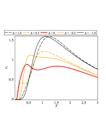
Finally, we discuss also another interesting thermodynamic quantity called the specific heat ($C=-T\partial^{2}f/\partial T^{2}$). In figure 4, we plot the specific heat as a function of the temperature $T$ for a fixed coupling parameter $J_{0}=1.0$ and a fixed value of $J=1.0$. By a solid line is represented the specific heat curve when $\Delta=0$, $0.5$ and $1.0$, while, for dashed line we illustrate the specific heat for $\Delta=-0.5$, and $-1.0$. For anisotropic parameter $\Delta=\pm 0.5$ and $0$, the plot illustrates a small anomalous peak due to the zero temperature phase transition influence, although for $\Delta=\pm 1.0$ this anomalous peak disappear, because there is no zero temperature phase transition in the neighborhood.

Figure 4: (Color online) Specific heat as a temperature dependency, for several values of anisotropic parameter assuming fixed values $J=1.0$ and $J_{0}=01.0$.

III.2 Pair correlation function

The nearest site correlation function between dimers can be obtained using a derivative of the free energy given by eq.(30). Then, in order to perform the derivative of free energy, we need to assume the parameter $J^{\prime}$ and $J$ as independent parameter, similarly $\Delta^{\prime}$ and $\Delta$ also are considered as independent parameters. Despite for physical quantities, the term $2J^{\prime}+\Delta^{\prime}$ in the free energy be irrelevant, this term cannot be neglected when we calculate the correlation function as expressed below:

$$\langle\sigma_{a}^{x}\sigma_{b}^{x}\rangle= -\frac{1}{2}\frac{\partial f}{\partial J^{\prime}}=-1+\frac{x^{\prime}}{2\lambda_{0}}\frac{\partial\lambda_{0}}{\partial x^{\prime}},$$ (31)

$$\langle\sigma_{a}^{z}\sigma_{b}^{z}\rangle= -\frac{\partial f}{\partial\Delta^{\prime}}=-1+\frac{z^{\prime}}{\lambda_{0}}\frac{\partial\lambda_{0}}{\partial z^{\prime}},$$ (32)

$$\langle\sigma_{c}^{x}\sigma_{d}^{x}\rangle= -\frac{1}{2}\frac{\partial f}{\partial J}=\frac{x}{2\lambda_{0}}\frac{\partial\lambda_{0}}{\partial x},$$ (33)

$$\langle\sigma_{c}^{z}\sigma_{d}^{z}\rangle= -\frac{\partial f}{\partial\Delta}=\frac{z}{\lambda_{0}}\frac{\partial\lambda_{0}}{\partial z}.$$ (34)

Here, we present the relation of the correlation function in terms of the largest eigenvalue of the transfer matrix $\lambda_{0}$.

Figure 5: Correlation functions for $ab$-dimer and $cd$-dimer defined by eqs. (31-34), assuming fixed parameter $J=1.0$ and $J_{0}=1.0$. (a) For the case of anisotropic parameter $\Delta=-0.3$. (b) And for the case of anisotropic parameter $\Delta=0.3$.

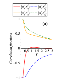
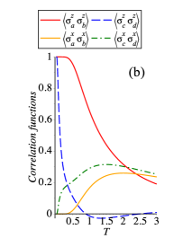
In order to accomplish our analysis concerning to the correlation function we display in fig.5 the correlation function given by eqs. (31-34), as a function of temperature, assuming convenientely fixed parameters $J_{0}=1.0$ and $J=1.0$ close to the phase transition illustrated in fig.2. Thus, in fig.5(a) we display for the case of anisotropic parameter $\Delta=-0.3$, and we observe how the correlation function at low temperature behaves quite similarly for both the $ab$-dimer and the $cd$-dimer; for example the $z$-component of pair correlation are negative because the ground state energy is TT(TS), while the $xy$-component are positive. However as soon the temperature increases the difference becomes relevant. It is worth to emphasize that the correlation function $\langle\sigma_{a}^{z}\sigma_{b}^{z}\rangle$ turn positive at finite temperature $T\approx 0.7$ and for higher temperature once again the correlation function is negative at a temperature of around $T\approx 2.5$ becoming a small negative amount. Similarly we also plot in fig.5(b) for anisotropic parameter $\Delta=0.3$, the $ab$-dimer and $cd$-dimer behaves quite similarly in the low temperature limit, the $z$-componet of pair correlation are positive because it corresponds to FM(AFM) region in agreement with eq.(11) and (12), while the $xy$-componet correlation function is zero. Nevertheless, for higher temperature this difference is significant, the $\langle\sigma_{a}^{x}\sigma_{b}^{x}\rangle$ and $\langle\sigma_{c}^{x}\sigma_{d}^{x}\rangle$ have a maximum at finite temperature, while the $\langle\sigma_{a}^{z}\sigma_{b}^{z}\rangle$ is a monotonic decreasing function and $\langle\sigma_{c}^{z}\sigma_{d}^{z}\rangle$ decreases faster becoming negative at $T\approx 0.9$ and for higher temperature at around $T\approx 2.4$ the $\langle\sigma_{c}^{z}\sigma_{d}^{z}\rangle$ correlation function becomes a positive quantity.

IV Thermal entanglement

Another interesting property we consider in this work, will be the quantum entanglement of the Ising-Heisenberg orthogonal dimer plaquette model. As a measure of entanglement for two arbitrary mixed states of dimers, we use the quantity called concurrencewooters , which is defined in terms of reduced density matrix $\rho$ of two mixed states

$$\mathcal{C}(\rho)=\max\{{0,2\Lambda_{max}-\text{{tr}}\sqrt{R}}\},$$ (35)

assuming

$$R=\rho\sigma^{y}\otimes\sigma^{y}\rho^{*}\sigma^{y}\otimes\sigma^{y},$$ (36)

where $\Lambda_{max}$ is the largest eigenvalue of the matrix $\sqrt{R}$ and $\rho^{*}$ represent the complex conjugate of matrix $\rho$, with $\sigma^{y}$ being the Pauli matrix.

For the case of infinite chain, the reduced density operator elementsbukman could be expressed in terms of the correlation function between two entangled particlesamico , consequently the concurrence between $ab$-dimer becomes

$$\mathcal{C}_{ab}=\max\{0,|\langle\sigma_{a}^{x}\sigma_{b}^{x}\rangle|-\frac{1}{2}|1+\langle\sigma_{a}^{z}\sigma_{b}^{z}\rangle|\},$$ (37)

similarly the concurrence between $cd$-dimer reads

$$\mathcal{C}_{cd}=\max\{0,|\langle\sigma_{c}^{x}\sigma_{d}^{x}\rangle|-\frac{1}{2}|1+\langle\sigma_{c}^{z}\sigma_{d}^{z}\rangle|\}.$$ (38)

Surely, we can obtain also equivalent result using the approach described in reference spra .

It is worthy to mention that the zero temperature entanglement for $ab$-dimer is maximally entangled in TS and TT region $\mathcal{C}_{ab}=1$, while, in all other region the $ab$-dimer becomes untangled ($\mathcal{C}_{ab}=0$). Whereas the $cd$-dimer also is maximally entangled in same (TS and TT) region $\mathcal{C}_{cd}=1$; additionally the DFA region now also becomes an entangled region whose concurrence is given by $\mathcal{C}_{cd}=\frac{|J|}{\sqrt{4J_{0}^{2}+J^{2}}}$ and it depends of $J$ and $J_{0}$. It is worth to notice, when $J=0$ this region becomes untangled, which is perfectly coherent since the model reduces to orthogonal plaquette Ising chain. Another special possibility is when $J_{0}=0$, the orthogonal dimer plaquette reduces simply to independent entangled dimers. While the FM and AFM region are untangled $\mathcal{C}_{cd}=0$.

Figure 6: (Color online) Concurrence for several values of anisotropic parameter as a function of $T$, assuming fixed $J_{0}=1$ and $J=1$. Dashed line corresponds for $ab$-dimer while the solid line represents $cd$-dimer.

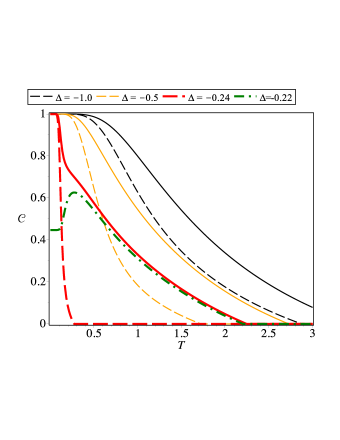
In figure 6 is plotted the concurrence $\mathcal{C}$ as a function of the temperature: for $\Delta=-1$ the dashed and solid line corresponds to $ab$-dimer and $cd$-dimer respectively. However, the $ab$-dimer entanglement vanishes for $T\approx 2.9$ while, for $cd$-dimer the entanglement vanishes at $T\approx 4$.0. For weaker anisotropic coupling ($\Delta$) this difference becomes more significantly, say i.e. for $\Delta=-0.24$, the $cd$-dimer (solid line) entanglement vanishes for $T\approx 2.25$, whilst for $ab$-dimer the entanglement vanishes at $T\approx 0.28$ (dashed line). For a bit weaker anisotropic parameter $\Delta=-0.22$, the $ab$-dimer becomes untangled region for any temperature, while $cd$-dimer entanglement vanishes at $T\approx 2.24$.

IV.1 Threshold temperature

The threshold temperature can be obtain when $ab$-dimer concurrence becomes null ($|\langle\sigma_{a}^{x}\sigma_{b}^{x}\rangle|=\frac{1}{2}|1+\langle\sigma_{a}^{z}\sigma_{b}^{z}\rangle|$), and similarly for $cd$-dimer, the concurrence will become null when ($|\langle\sigma_{c}^{x}\sigma_{d}^{x}\rangle|=\frac{1}{2}|1+\langle\sigma_{c}^{z}\sigma_{d}^{z}\rangle|$).

Figure 7: Threshold temperature $T_{th}$ as a function of $\Delta$, for fixed $J_{0}=1$ and $J=1$. Dashed line corresponds for $ab$-dimer, while the solid line represents $cd$-dimer.

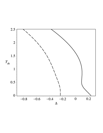
The threshold temperature is illustrated in figure 7 as a function of anisotropic parameter for fixed values of $J_{0}=1$ and $J=1$. The dashed line correspond for the $ab$-dimer threshold temperature, and in the low temperature limit, the threshold temperature leads to $T_{th}=2-\sqrt{5}$. Whereas the solid line represents the $cd$-dimer threshold temperature; in the low temperature limit it leads to $T_{th}=\sqrt{5}-2$. It is worthy to highlight that the threshold temperature for $cd$-dimer exhibits a thin reentrance around to $\Delta=0.1$.

Another way to display the entanglement phase diagram is in units of threshold temperature as displayed in figure 8, the boundary between entangled region and untangled region is given by a solid (red) line. The black region correspond to maximally entangled region, and white region corresponds to untangled region, while light gray region corresponds to weak concurrence, similarly dark gray corresponds to strong concurrence. The entangled phase diagram $J$ against $\Delta$ in units of $T_{th}$, behaves quite similar for both $ab$-dimer and $cd$-dimer, although, for $ab$-dimer the untangled region appears already significantly for $\Delta\geqslant-3$ and small values of $J$, while for $cd$-dimer the untangled region becomes relevant only for $\Delta\geqslant-1$ and small values of $J$. Certainly this is in agreement with the zero temperature phase diagram displayed in figure 2(a).

Figure 8: (Color online) Density plot of concurrence in units of $T_{th}$, darkest region corresponds to higher entanglement. (a) Concurrence for $ab$-dimer as a dependency of $J$ and $\Delta$ for a fixed value of $J_{0}=1$. (b) Concurrence for $cd$-dimer as a dependency of $J$ and $\Delta$ for a fixed value of $J_{0}=1$.

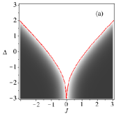
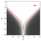
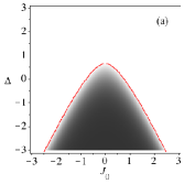
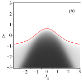
Additional density plot of entangled phase diagram is displayed in figure 9 in terms of $\Delta$ and $J_{0}$, once again in units of $T_{th}$, the phase diagrams for $ab$-dimer is given in fig.2(a), and the phase diagram for $cd$-dimer is illustrated in fig.2(b). Here, we observe the phase diagram between $ab$-dimer and $cd$-dimer are quite different, but still are closely related to the zero temperature phase diagram illustrated in figure 2(b). Although the darkest (strongly entangled) region are very similar for both dimers.

Figure 9: Density plot of Concurrence in units of $T_{th}$, darkest rebaxter-book region corresponds to higher entanglement. (a) Concurrence for $ab$-dimer as a dependency of $J_{0}$ and $\Delta$ for a fixed value of $J=1$. (b) Concurrence for $cd$-dimer as a dependency of $J_{0}$ and $\Delta$ for a fixed value of $J=1$.

V Conclusion

In this work, we studied the dimer-plaquette Ising-Heisenberg chain, assembled between plaquette edge also known as orthogonal dimer plaquetteivanov ; richter ; schu ; koga ; koga02 ; vadim12 . Using the local gauge symmetry of this model, we are able to map onto a simple spin-1 like Ising and spin-1/2 Heisenberg dimer model with single effective ion anisotropy. Thereafter, this model can be solved using the decoration transformationSyozi ; Fisher ; phys-A-09 ; JPA-11 and transfer matrix approach. First we discuss the phase diagram at zero temperature of this model, where we found five ground states as illustrated in figure 2, one ferromagnetic, one antiferromagnetic, one triplet-triplet disordered and triplet-singlet disordered phase, beside a dimer ferromagnetic-antiferromagnetic phase. It is interesting to remark that, in the limit of pure Ising model this exhibits a frustrated region. Furthermore, the thermodynamic properties are discussed such as entropy, specific heat as well as the correlation function. Additionally, using the nearest site correlation function it is possible to analyze the pairwise thermal entanglement for both $ab$-dimer and $cd$-dimer, as well as the threshold temperature of the entangled region are discussed as a function of the Hamiltonian parameters. There is some significant difference between both dimers ($ab$-dimers and $cd$-dimers) which is in agreement in the low temperature limit. However, for strong entanglement, both dimers are quite similar. As a consequence of this difference, we can illustrate one interesting result, regarding to the reentrance type of threshold temperature for $cd$-dimer, despite for $ab$-dimer there is no reentrance temperature.