The moduli space of striped black branes
Benjamin Withers
Centre for Particle Theory and Department of Mathematical Sciences
Durham University, South Road, Durham, DH1 3LE, U.K.
Abstract
At finite charge density certain holographic models exhibit the spontaneous breaking of translational invariance resulting in an inhomogeneous phase. We follow up on recent numerical work, reporting results for a larger class of cohomogeneity two black branes in AdS, dual to a holographic striped phase. We construct the continuous moduli space of inhomogeneous black branes as a function of the temperature. Minimising the free energy we determine the dominant striped solutions, revealing a growth in the stripe size as the system is cooled. We discuss the thermodynamic properties of this line of solutions.
1 Introduction
There is great interest in applying the holographic framework to systems which may be of relevance to real-world condensed matter phenomena, with one focus placed on equilibrium phases at finite charge density and temperature. An early example is provided by the holographic description of a superfluid, which can be built with the minimal addition of a charged scalar field to the bulk gravitational theory. The scalar may be added in a phenomenological fashion [1, 2, 3] or by seeking appropriate consistent truncations of supergravity reductions [4, 5]. The superfluid phase transition in the CFT is described in the bulk by a branch of thermodynamically preferred black branes with scalar condensate connecting with the normal phase.
There is growing evidence that symmetry breaking phases may be generic in holography at finite charge density. In particular, linear analyses indicate the spontaneous breaking of the Euclidean group of symmetries [6, 7, 8, 9] in a variety of gravitational settings [10, 11, 12, 13] as well as probe brane constructions [14, 15, 16, 17]. To establish whether a phase transition exists, construction of the broken solutions beyond linear order is necessary, which typically requires the solution of PDEs. In cases where the broken phase retains homogeneity, fully backreacted solutions have been constructed by solving ODEs [18, 19, 20] exhibiting the emergence of a thermodynamically preferred spatial scale, associated with helical order. Such solutions provide an important set of examples for comparison with inhomogeneous solutions.
Recently the first examples showing continuous phase transitions to an inhomogeneous phase in this context were presented in [21, 22] (see also [23]), in the Einstein-Maxwell-pseudoscalar bulk models studied perturbatively in [8]. There, a branch of solutions at fixed periodicity was considered, connecting with a single striped zero-mode of the RN background with wavenumber . In this paper we relax the condition of fixed , finding a continuous moduli space of striped solutions at each temperature. In particular, we consider the natural generalisation of the solutions constructed in [21, 22], by seeking the nonlinear one-parameter families which emerge from a given striped zero-mode, , for all . In this way we construct a two-parameter family of solutions labelled by the dimensionless temperature, , and periodicity scale, .
For an infinite translationally invariant system at temperature , the physically relevant solutions in this space are those which minimise the free energy. These can be labelled by their periodicity, giving rise to the curve . Considering this line of solutions we find a second order phase transition from the homogeneous phase. In the helical case [19, 20] it was found that the dominant scale at any given temperature was characterised by the vanishing of a particular piece of boundary data. We will uncover an analogous result for inhomogeneous solutions constructed here, in one lower dimension.
2 The setup of [22]
In this section we briefly recap the model and numerical setup of [22]. We adopt a bulk model studied in [8] containing a neutral pseudo-scalar, , a single gauge field, with field strength , and crucially in this context, a parity-violating coupling, ,
| (2.1) |
where we have set . In this paper we study a single case, taking , and . When this phenomenological model becomes a consistent truncation of a reduction from 11D on SE7 [25, 26, 27]. Here we adopt the slightly higher value of which raises the critical temperature for the striped instability. We seek regular stationary solutions within the bulk metric ansatz
| (2.2) |
and gauge field , where and are functions both of the AdS radial coordinate, , and a single spatial boundary direction with translational invariance in . The function conveniently factors out the normal phase solution, an electrically charged Reissner-Nordstrom (RN) black brane branch at and and . The coordinate runs from at the boundary to at the (non-degenerate) horizon. To render the system elliptic we adopt the Harmonic Einstein equation approach of [29, 30, 31] and we employ a spectral method with grid points in the bulk. Further details can be found in [22]. For the data presented in this paper we have taken for , for , for , for and finally for .
The non-vanishing components of the expectation value of the CFT stress tensor and current are given by,
| (2.3) | |||||
| (2.4) | |||||
| (2.5) | |||||
| (2.6) |
| (2.7) | |||||
| (2.8) |
where denotes the coefficient of in the small- boundary expansion of the field . Note that the stress tensor is traceless and is constant in , following from conservation of the stress tensor. Spatial averages of these quantities will be denoted with a bar.
3 Striped zero-modes
We begin with a summary of the striped zero-modes on the RN normal phase solution, following [8]. These modes indicate the boundary of stability for the RN solution, providing a starting point for the construction of an emergent family of nonlinear striped black branes. Moreover, in this model at any temperature the boundary of stability will coincide with the boundary of existence for the striped solutions (labelled by their periodicity), as we shall show in the following section.
Consider a single Fourier mode with wavenumber for the following perturbations,
| (3.1) |
with the others set at their RN values. The resulting equations at are three second order k-dependent linear ODEs. With the conditions of horizon regularity and normalisability in the UV, counting the number of pieces of boundary data reveals that there can be at most discrete striped zero-modes at a given . In particular for there are two zero-modes at fixed , giving rise to the characteristic critical temperature ‘bell curve’ presented in figure 1.
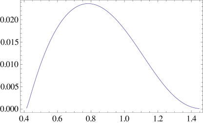
As the system is cooled we first encounter a single zero-mode at at the scale . Thus the natural strategy for constructing nonlinear solutions is to consider those solutions which are continuously connected to this mode. In particular, in the next section we consider those solutions which emerge from starting with a single zero-mode of wavenumber and lowering the temperature. This gives rise to a two parameter family of solutions labelled by and .
As a side remark, as there are two zero-modes at temperatures , a second possibility is that there are additional branches of nonlinear solutions which connect with a superposition of them. In the numerical method used we must fix the periodicity of the solution and so this scenario is largely excluded, except at a discrete set of temperatures for which the higher zero-mode wavenumber is an integer multiple of the lower. We have not constructed any solutions of this type, though we anticipate that if they do exist they will be thermodynamically subdominant.
4 Nonlinear solutions
If we fix the periodicity of the solution and lower the temperature then [22] (see also [21] for similar models) showed the existence of a second order phase transition. More generally though, as discussed in section 3, there is a two parameter family of solutions connecting with the RN branch along the line of striped zero-modes shown in figure 1. Here we construct these solutions and investigate the thermodynamically preferred stripe as a function of the temperature, .
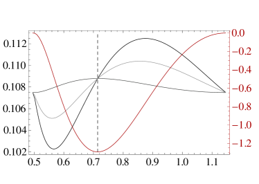
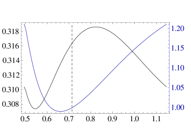
We begin by considering the space of such solutions which exist at a fixed temperature , for which various averaged thermodynamic quantities are shown in figure 2. First we note that the striped solutions exist within the interval defined by the locations of the two zero-modes at this temperature. Additionally we see that the free energy and the entropy of the striped phase is always lower than the RN value. Note that the thermodynamically preferred striped solution at this temperature appears to have the property , and we will discuss this shortly. The relationship between and follows from conformality.
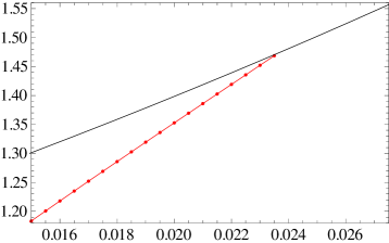
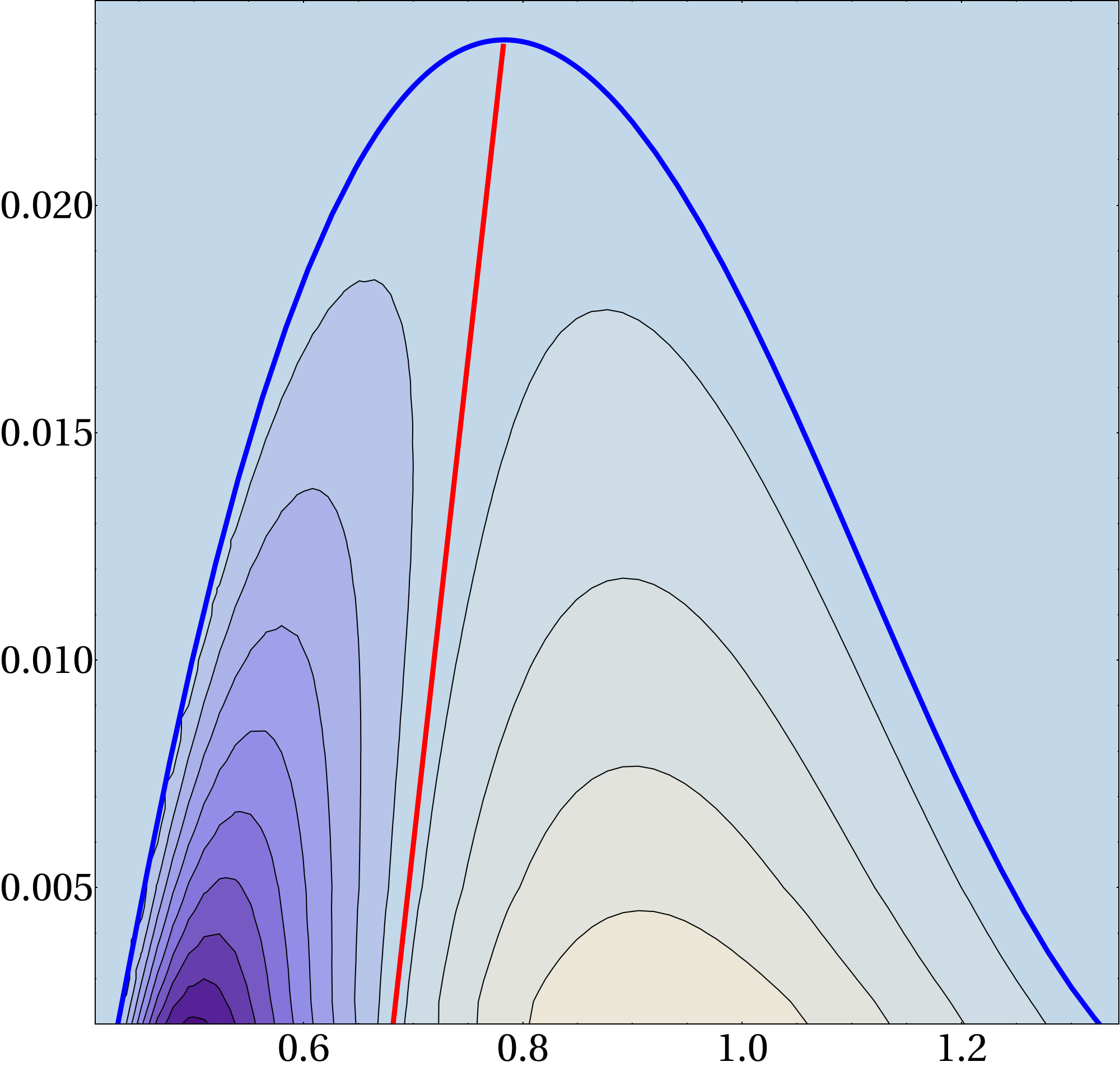
Extending this analysis to the two parameter family, in figure 3 we show the averaged free energy where the RN value has been subtracted. We have only found striped solutions below the threshold temperature, indicated in blue, where they dominate.111See however, an example of a different model in [22] where solutions at higher temperatures were found. Outside this region we have simply plotted the RN values. Considering the system at any fixed we see that there is a continuous phase transition to the broken phase, as seen for a specific value in [22]. However, as emphasised we should determine the preferred as a function of the temperature. This locus of solutions is given by the red line in figure 3. For clarity we also plot the dominant in figure 4, showing a monotonic growth in the stripe size as the temperature is reduced. Furthermore it approaches a non-zero value at low temperatures.
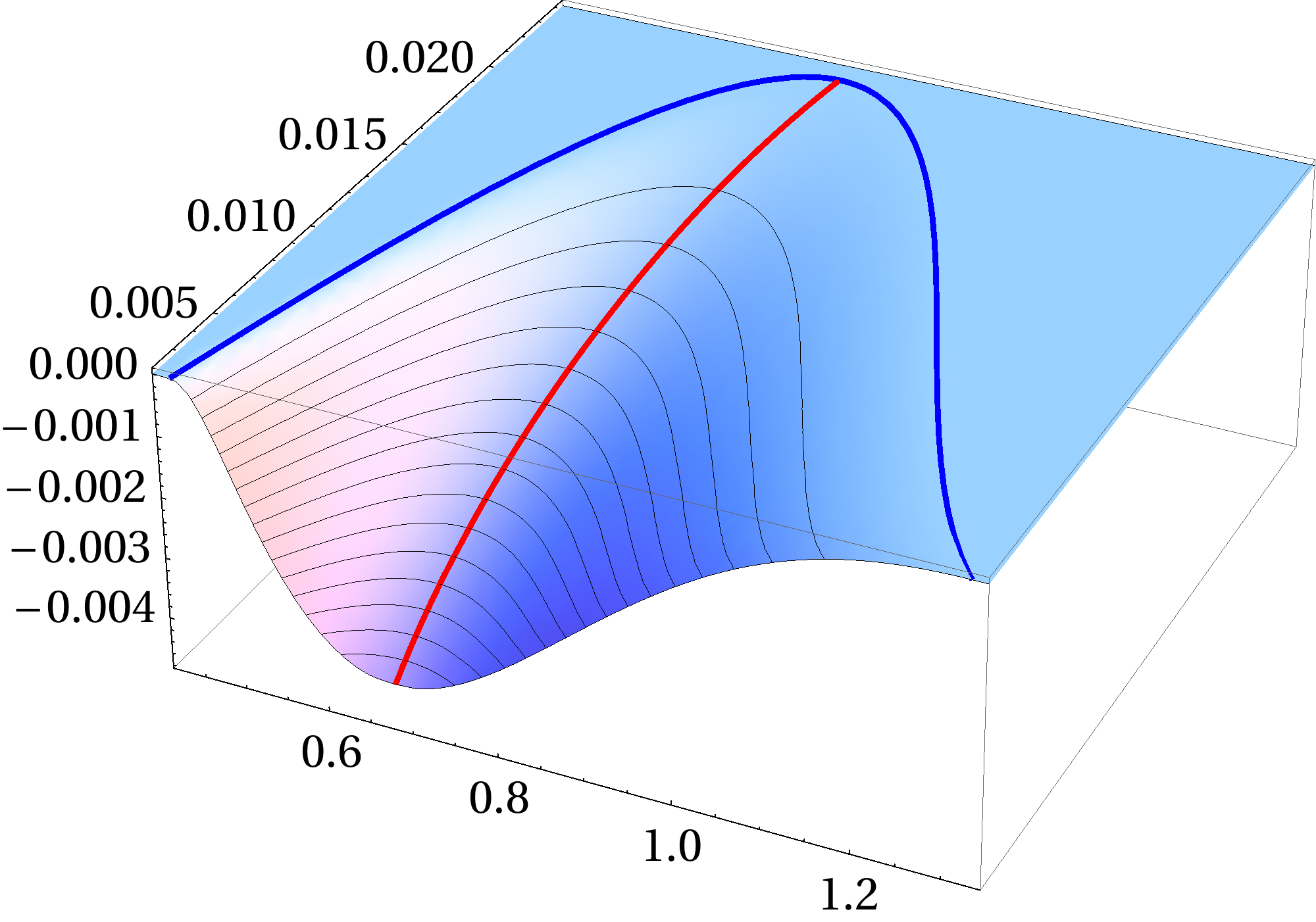
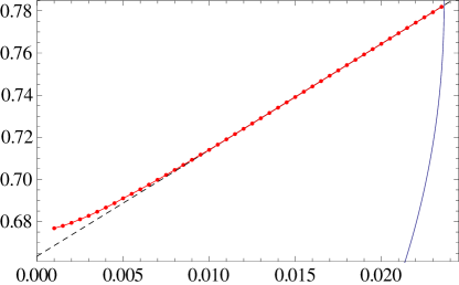
We now restrict our attention to this preferred line of solutions. Again, we see that there is a continuous phase transition, illustrated by the free energy shown in figure 5. Figure 6 shows the entropy density, which via the first law indicates a that the transition is second order. Following the system to lower temperatures, , we see evidence of a zero entropy state emerging at zero temperature.
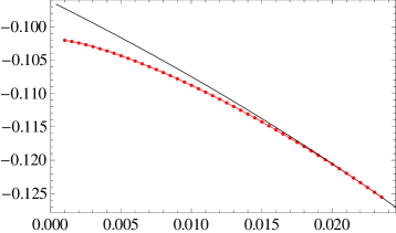
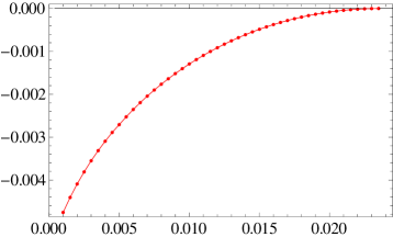
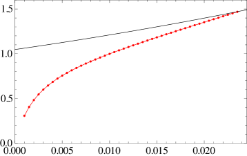
For the five-dimensional helical black branes constructed in [19, 20], it was found that the thermodynamically preferred solutions at fixed temperature were characterised by the vanishing of a particular quantity in the boundary stress tensor. Here we work in four dimensions, and we seek a analogous statement. One way of characterising the vanishing quantity of [19, 20] is through the relation in the case where the stress tensor depends on the coordinate and is the spatial dimension of the boundary.222In the notation of [19, 20], whilst the relation amounts to the vanishing of the boundary data . Indeed, we find that along the preferred line of inhomogeneous solutions studied in this paper, this relation holds within numerical accuracy, and is not satisfied away from this locus. This is clearly demonstrated for the space of solutions at the fixed shown in figure 2. This is equivalent to the relation amongst averaged boundary data, . For all solutions presented in this paper we find that the spatial average of and vanishes, consistent with the perturbative structure [8]. Consequently if the relation is satisfied, then conformality implies that both the spatially averaged stress tensor and spatially averaged current are isotropic. In order to numerically test this relation more comprehensively, it is convenient to define the dimensionless ratio,
| (4.1) |
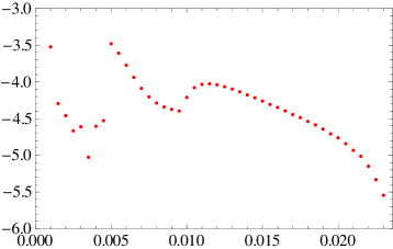
In figure 7 we plot this quantity for the two parameter family of black branes. In general, , but we find that it vanishes along the line of thermodynamically preferred solutions.
5 Final comments
We have constructed a two-parameter family of cohomogeneity-two black brane solutions with AdS4 asymptotics, dual to a phase at finite charge density with spontaneously broken translational invariance in one direction. The family may be described as a space of solutions labelled by their periodicity in one of the spatial boundary directions, , at each temperature . This work builds on the results [22] (see also [21]) where second order phase transitions were found for one parameter families at fixed in this model.
In section 4, for the two parameter family, we find continuous phase transitions at the threshold of the linear striped instabilities. In other words, if we were to fix the periodicity of the system somehow, then the phase boundary would be given by the zero-mode analysis, illustrated by the characteristic ‘bell curve’ in figure 1. However, in the absence of such a restriction we are interested in those solutions which minimise the free energy at a given temperature, . Constructing this set of solutions, we have found the preferred scale as a function of temperature , with the stripe size monotonically growing as the temperature is reduced, approaching a non-zero value at low temperatures.
We also examined the properties of this preferred set of solutions. As in the fixed case, we have shown that the system exhibits a second order phase transition to the inhomogeneous phase, with the entropy appearing to vanish as the inhomogeneous zero temperature state is approached. Constructing these states directly at zero temperature would be profitable. Motivated by an analogous feature in the helical black brane setting [19, 20] we have examined a particular combination of stress-tensor components, . We find that whilst is non-zero in general for the two parameter family, it vanishes along the line of solutions which dominate the ensemble at fixed . In this case, vanishing implies isotropy of the spatially-averaged stress tensor. It would be interesting to investigate the origin of this feature.
Finally, we stress that we have focussed on cohomogeneity-two solutions. More generally we anticipate that there is a cohomogeneity-three family of solutions emerging from the bell-curve (figure 1), which may turn out to dominate the ensemble.
Acknowledgements
We thank Aristomenis Donos, Jerome Gauntlett, Julian Sonner and Toby Wiseman for useful discussions. We thank the Perimeter Institute and Nordita for hospitality. This work is supported by a Royal Commission for the Exhibition of 1851 Science Research Fellowship.
References
- [1] S. S. Gubser, “Breaking an Abelian Gauge Symmetry Near a Black Hole Horizon,” Phys. Rev. D78 (2008) 065034, arXiv:0801.2977 [hep-th].
- [2] S. A. Hartnoll, C. P. Herzog, and G. T. Horowitz, “Building a Holographic Superconductor,” Phys. Rev. Lett. 101 (2008) 031601, arXiv:0803.3295 [hep-th].
- [3] S. A. Hartnoll, C. P. Herzog, and G. T. Horowitz, “Holographic Superconductors,” JHEP 12 (2008) 015, arXiv:0810.1563 [hep-th].
- [4] J. P. Gauntlett, J. Sonner, and T. Wiseman, “Holographic superconductivity in M-Theory,” Phys. Rev. Lett. 103 (2009) 151601, arXiv:0907.3796 [hep-th].
- [5] S. S. Gubser, C. P. Herzog, S. S. Pufu, and T. Tesileanu, “Superconductors from Superstrings,” Phys. Rev. Lett. 103 (2009) 141601, arXiv:0907.3510 [hep-th].
- [6] S. Nakamura, H. Ooguri, and C.-S. Park, “Gravity Dual of Spatially Modulated Phase,” Phys. Rev. D81 (2010) 044018, arXiv:0911.0679 [hep-th].
- [7] H. Ooguri and C.-S. Park, “Holographic End-Point of Spatially Modulated Phase Transition,” Phys. Rev. D82 (2010) 126001, arXiv:1007.3737 [hep-th].
- [8] A. Donos and J. P. Gauntlett, “Holographic striped phases,” JHEP 1108 (2011) 140, arXiv:1106.2004 [hep-th].
- [9] A. Donos and J. P. Gauntlett, “Holographic helical superconductors,” JHEP 12 (2011) 091, arXiv:1109.3866 [hep-th].
- [10] D. Vegh, “Holography without translational symmetry,” arXiv:1301.0537 [hep-th].
- [11] A. Donos and J. P. Gauntlett, “Holographic charge density waves,” arXiv:1303.4398 [hep-th].
- [12] S. Cremonini and A. Sinkovics, “Spatially Modulated Instabilities of Geometries with Hyperscaling Violation,” arXiv:1212.4172 [hep-th].
- [13] N. Iizuka and K. Maeda, “Stripe Instabilities of Geometries with Hyperscaling Violation,” arXiv:1301.5677 [hep-th].
- [14] S. K. Domokos and J. A. Harvey, “Baryon number-induced Chern-Simons couplings of vector and axial-vector mesons in holographic QCD,” Phys. Rev. Lett. 99 (2007) 141602, arXiv:0704.1604 [hep-ph].
- [15] H. Ooguri and C.-S. Park, “Spatially Modulated Phase in Holographic Quark-Gluon Plasma,” Phys. Rev. Lett. 106 (2011) 061601, arXiv:1011.4144 [hep-th].
- [16] C. A. B. Bayona, K. Peeters, and M. Zamaklar, “A non-homogeneous ground state of the low-temperature Sakai-Sugimoto model,” JHEP 06 (2011) 092, arXiv:1104.2291 [hep-th].
- [17] O. Bergman, N. Jokela, G. Lifschytz, and M. Lippert, “Striped instability of a holographic Fermi-like liquid,” JHEP 10 (2011) 034, arXiv:1106.3883 [hep-th].
- [18] N. Iizuka, S. Kachru, N. Kundu, P. Narayan, N. Sircar, et al., “Bianchi Attractors: A Classification of Extremal Black Brane Geometries,” arXiv:1201.4861 [hep-th].
- [19] A. Donos and J. P. Gauntlett, “Helical superconducting black holes,” Phys.Rev.Lett. 108 (2012) 211601, arXiv:1203.0533 [hep-th].
- [20] A. Donos and J. P. Gauntlett, “Black holes dual to helical current phases,” arXiv:1204.1734 [hep-th].
- [21] A. Donos, “Striped phases from holography,” arXiv:1303.7211 [hep-th].
- [22] B. Withers, “Black branes dual to striped phases,” arXiv:1304.0129 [hep-th].
- [23] M. Rozali, D. Smyth, E. Sorkin, and J. B. Stang, “Holographic Stripes,” arXiv:1211.5600v1 [hep-th].
- [24] M. Rozali, D. Smyth, E. Sorkin, and J. B. Stang, “Holographic Stripes,” arXiv:1211.5600v2 [hep-th].
- [25] J. P. Gauntlett, J. Sonner, and T. Wiseman, “Quantum Criticality and Holographic Superconductors in M- theory,” JHEP 02 (2010) 060, arXiv:0912.0512 [hep-th].
- [26] J. P. Gauntlett, S. Kim, O. Varela, and D. Waldram, “Consistent Supersymmetric Kaluza–Klein Truncations with Massive Modes,” JHEP 04 (2009) 102, arXiv:0901.0676 [hep-th].
- [27] A. Donos, J. P. Gauntlett, J. Sonner, and B. Withers, “Competing orders in M-theory: superfluids, stripes and metamagnetism,” JHEP 1303 (2013) 108, arXiv:1212.0871 [hep-th].
- [28] V. Balasubramanian and P. Kraus, “A stress tensor for anti-de Sitter gravity,” Commun. Math. Phys. 208 (1999) 413–428, arXiv:hep-th/9902121.
- [29] M. Headrick, S. Kitchen, and T. Wiseman, “A New approach to static numerical relativity, and its application to Kaluza-Klein black holes,” Class.Quant.Grav. 27 (2010) 035002, arXiv:0905.1822 [gr-qc].
- [30] A. Adam, S. Kitchen, and T. Wiseman, “A numerical approach to finding general stationary vacuum black holes,” Class.Quant.Grav. 29 (2012) 165002, arXiv:1105.6347 [gr-qc].
- [31] T. Wiseman, “Numerical construction of static and stationary black holes,” arXiv:1107.5513 [gr-qc].
- [32] G. T. Horowitz, J. E. Santos, and D. Tong, “Optical Conductivity with Holographic Lattices,” JHEP 1207 (2012) 168, arXiv:1204.0519 [hep-th].
- [33] G. T. Horowitz, J. E. Santos, and D. Tong, “Further Evidence for Lattice-Induced Scaling,” JHEP 1211 (2012) 102, arXiv:1209.1098 [hep-th].
- [34] G. T. Horowitz and J. E. Santos, “General Relativity and the Cuprates,” arXiv:1302.6586 [hep-th].