Fluctuation dynamo amplified by intermittent shear bursts in convectively driven magnetohydrodynamic turbulence

Intermittent large-scale high-shear flows are found to occur frequently and spontaneously in direct numerical simulations of statistically stationary turbulent Boussinesq magnetohydrodynamic (MHD) convection. The energetic steady state of the system is sustained by convective driving of the velocity field and small-scale dynamo action. The intermittent emergence of flow structures with strong velocity and magnetic shearing generates magnetic energy at an elevated rate over time scales longer than the characteristic time of the large-scale convective motion. The resilience of magnetic energy amplification suggests that intermittent shear bursts are a significant driver of dynamo action in turbulent magnetoconvection.

1 Introduction

X-ray observations reveal that turbulent convection agitates the outer convection layer of stars (Güdel et al., 1997; Reiners & Basri, 2007; Böhm-Vitense, 2008; Simon et al., 2008). Measurements also show that planetary magnetic fields can change in magnitude and orientation (McFadden & Merrill, 1995; Christensen et al., 2009; Stevenson, 2010; Olson et al., 2011). Dynamo action driven by turbulent convection is accepted as the origin of solar and planetary magnetic fields. Key physical processes involved in turbulent convection and implicated in the amplification of magnetic fields remain to be identified and practically understood (Zeldovich et al., 1983; Biskamp, 2003). Helicity, shear, and buoyancy remain intensely interesting to the dynamo problem (Tobias, 2009; Wicht & Tilgner, 2010; Weiss & Thompson, 2009).

Because of the inherent nonlinearity of turbulent plasma flows, theoretical explanation of dynamo action is often approached by mean-field theory. Comparison with three-dimensional numerical simulations verifies and inspires theoretical models (Moll et al., 2011; Schrinner et al., 2005, 2007; Wilkin et al., 2007; Harder & Hansen, 2005; Stanley & Glatzmaier, 2010; Tobias et al., 2011). This work reports on a resilient and newly identified feature of characteristic dynamo action in three-dimensional, convectively driven, homogeneously turbulent, Boussinesq magnetoconvection based on pseudospectral direct numerical simulations using the magnetohydrodynamic (MHD) fluid approximation (Chandrasekhar, 1961).

2 Simulation

Formulation of optimal boundary conditions for simulations of turbulent flows is delicate because boundaries strongly influence the structure and dynamics of the flow. The commonly used Rayleigh Bénard boundary conditions impose a temperature gradient to drive turbulent convection by fixing the temperature on impermeable top and bottom boundaries. For the Reynolds and Rayleigh numbers achievable with current numerical capabilities, the convection-cell pattern imposed on the flow by Rayleigh Bénard boundary conditions constrains the development of buoyantly driven turbulence.

The simulation volume considered in this work is confined by quasi-periodic rather than Rayleigh Bénard boundary conditions. The only deviation from full periodicity in the quasi-periodic boundary conditions is the explicit suppression of mean flows parallel to gravity, which are removed at each time step. Because our simulations are pseudospectral, the mean flow is straightforwardly isolated as the $k=0$ mode in Fourier space, which corresponds to the volume-averaged velocity. The aim is to combine the conceptual simplicity of statistical homogeneity with a physically natural convective driving of the turbulent flow. In the flow allowed by the quasi-periodic boundary conditions we identify a process, the shear burst, in our simulation that efficiently amplifies magnetic energy at all spatial scales in convective turbulence. This process can be relatively subtle, but arises in all cases considered in this work. The simulation model we employ is idealized, but can be viewed as a volume in an astrophysical or geophysical convective turbulent flow that is small in comparison to the pressure scale height.

Our system allows the study of a turbulent fluctuation dynamo (also known as a small-scale dynamo) in detail since the applied boundary conditions permit shear bursts on large spatial and temporal scales without enforcing a large-scale structuring of the turbulent flow. Hundreds of convective time scales prove necessary for the study of the shear bursts that arise spontaneously in simulations of steady-state convective MHD turbulence. Shear bursts are intermittent and spatially localized around high-shear flows. They are driven primarily at multiple large length scales that do not necessarily form a continuous band in wavenumber space, and that vary between bursts. A single isolated burst is not sufficient to maintain elevated magnetic energy; however, shear bursts can sometimes recur frequently, as shown in Fig. 1, providing an elevated growth of magnetic energy over significant periods of time. We address the properties of shear bursts and their importance for the understanding of the fluctuation-dynamo mechanism based on observations from high-resolution direct numerical simulations that span extended periods of time.

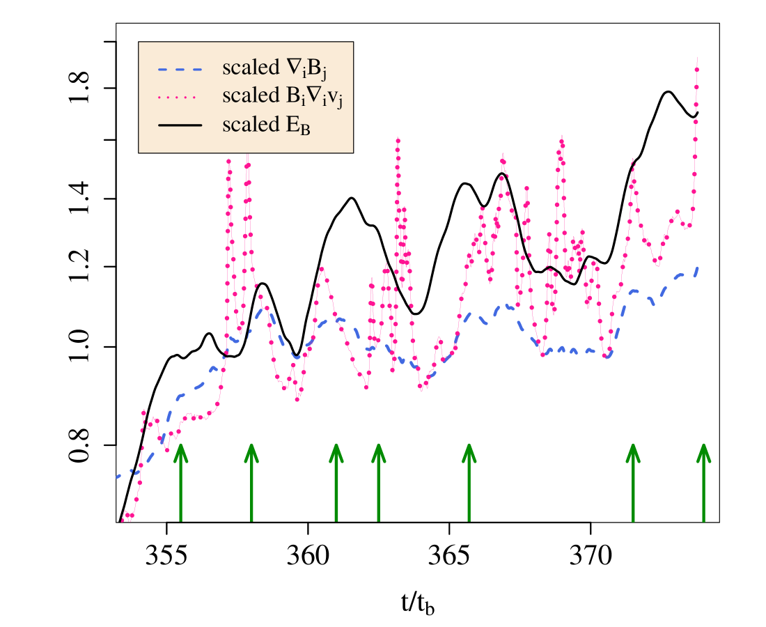
Figure 1: Magnetic energy, $E_{\mathrm{B}}$, is significantly amplified over long times due to repeated shear bursts in (above) simulation g1 and (below) simulation g11 (parameters described in Table 1). The signature of the shear burst, identified here with arrows, is clearly visible in the simultaneous peaks of the magnitude of the magnetic shear tensor $\nabla_{i}B_{j}$, and magnetic stretching tensor $B_{i}\nabla_{i}u_{j}$, which have been normalized to their initial-time values for easy comparison. The magnitude of the velocity shear tensor $\nabla_{i}v_{j}$ closely follows the magnetic shear. The magnitude of these tensors is calculated as a sum of the squares of the elements. Shear, and therefore magnetic stretching, drive the intermittent growth of magnetic energy.

The non-dimensional Boussinesq equations for MHD convection are

$$\frac{\partial\mbox{\boldmath$\omega$}}{\partial t} - \nabla\times(\mbox{\boldmath$v$}\times\mbox{\boldmath$\omega$}+\mbox{\boldmath$j$}\times\mbox{\boldmath$B$})=\hat{\nu}\nabla^{2}\mbox{\boldmath$\omega$}-\nabla\theta\times\mbox{\boldmath$g$}_{0}$$ (1)

$$\frac{\partial\mbox{\boldmath$B$}}{\partial t} - \nabla\times(\mbox{\boldmath$v$}\times\mbox{\boldmath$B$})=\hat{\eta}\nabla^{2}\mbox{\boldmath$B$}$$ (2)

$$\frac{\partial\theta}{\partial t} + (\mbox{\boldmath$v$}\cdot\nabla)\theta=\hat{\kappa}\nabla^{2}\theta-(\mbox{\boldmath$v$}\cdot\nabla)T_{0}$$ (4)

$$\nabla\cdot\mbox{\boldmath$v$}=\nabla\cdot\mbox{\boldmath$B$}=0\leavevmode\nobreak\ \leavevmode\nobreak\ .$$

The equations include the solenoidal velocity field $v$, vorticity $\mbox{\boldmath$\omega$}=\nabla\times\mbox{\boldmath$v$}$, magnetic field $B$, and current $\mbox{\boldmath$j$}=\nabla\times\mbox{\boldmath$B$}$. The quantity $\theta$ denotes the temperature fluctuation about a linear mean temperature profile $T_{0}(z)$ where $z$ is the direction of gravity. In equation 4 this mean temperature provides the convective drive of the system. In eq. 1, the term including the temperature fluctuation $\theta$ is the buoyancy force. The vector $\mbox{\boldmath$g$}_{0}$ is a unit vector in the direction of gravity. These equations are solved using a pseudospectral method with an adaptive time integration accomplished by a low-storage third-order Runge Kutta scheme (Williamson, 1980).

Turbulent convective motion defines the characteristic time and length scales of the system: the large-scale buoyancy time, $t_{\mathrm{b}}=(\alpha g|\nabla T_{0}|)^{-1/2}$ and temperature gradient length scale $\mathsf{L}=T_{*}/\nabla T_{0}$ where $T_{*}$ is defined as the root-mean-square of temperature fluctuations $\theta$. The volume thermal expansion coefficient at constant pressure is $\alpha$, and the gravitational acceleration is $g$ (Gibert et al., 2006; Škandera & Müller, 2009). The magnetic field is given in Alfvénic units, with Alfvén Mach number $v_{0}/v_{\mathrm{A}}=1$, $v_{0}=\mathsf{L}/t_{\mathrm{b}}$. Three dimensionless parameters appear in the equations: $\hat{\nu}$, $\hat{\eta}$, and $\hat{\kappa}$. They derive from the kinematic viscosity $\nu$, the magnetic diffusivity $\eta$, and thermal diffusivity $\kappa$ and can formally be identified as the reciprocal value of classical Reynolds number, magnetic Reynolds number, and Péclet numbers, respectively (see Table 1 for definitions).

To investigate the influence of diffusivities on the shear burst phenomena, parameters $\hat{\nu}$, $\hat{\eta}$, and $\hat{\kappa}$ are varied; consequently the simulations probe values of the Prandtl $\mathsf{Pr}=\hat{\nu}/\hat{\kappa}$ and the magnetic Prandtl number $\mathsf{Pr_{m}}=\hat{\nu}/\hat{\eta}$ spread between 0.5 and 2. The magnetic Prandtl number has been shown to exhibit a significant effect on small-scale dynamo action (Boldyrev & Cattaneo, 2004; Schekochihin et al., 2005); the dependence of the dynamo mechanism on Prandtl number has been the subject of several wide-ranging investigations (Schmalzl et al., 2002; Maron et al., 2004; Simitev & Busse, 2005). Realistically small Prandtl numbers cannot be reached with contemporary computer capabilities; in the solar convection zone expected values are $\mathsf{Pr_{m}}\sim 10^{-4}$ – $10^{-7}$ and in the earth’s core $\mathsf{Pr_{m}}\sim 10^{-6}$. Simultaneously, Reynolds numbers are generally expected to be larger than can be computationally reached: $\mathsf{Re}\sim 10^{13}$ in the solar convection zone and $\mathsf{Re}\sim 10^{8}$ in the earth’s core (summarized in Busse, 2009). Because of this discrepancy, the dynamical ranges of fluctuations in modern simulations are smaller than those expected in real systems. Our simulations thus present a first impression of the role of shear bursts for astrophysical dynamos.

Figure 2: Total kinetic, magnetic and thermal energies during the initial growth phase of the dynamo in simulation g2.

3 Results

The numerical turbulence data in this work results from a set of simulations conducted with grid size $512^{3}$, which constitutes high resolution for the extremely long times treated here. These simulations are performed in a quasi-periodic slab or cube; the cube has a side of $2\pi$, and the slab has slightly larger $x$- and $y$-directions of $(2\pi)^{3/2}$ to allow for the well-defined initial onset of the convective instability driving the turbulence (Chandrasekhar, 1961). Our boundary conditions inhibit the formation of viscous boundary layers, which appear when impermeable boundary conditions are employed. The dissipative coefficients $\hat{\nu}$, $\hat{\eta}$, and $\hat{\kappa}$ parametrize the extent of the turbulent inertial range of scales, and in each simulation are chosen to be as small as possible so that the resolution constraint of $k_{\mathrm{max}}\eta_{\mathsf{kol}}>1.5$ is still satisfied (Pope, 2000). Here, $k_{\mathrm{max}}$ is the largest resolvable wavenumber allowed by numerical resolution and $\eta_{\mathsf{kol}}$ is the Kolmogorov length scale. We performed simulations for the wide range of parameters summarized in Table 1 in order to test for a possible dependence of the shear burst phenomenon on the Reynolds numbers and Prandtl numbers. Shear bursts occurred in all of the simulations listed. The Rayleigh number, characterizing the dynamical importance of buoyancy in Rayleigh-Bènard configurations, is of limited informative value for the present quasi-periodic system.

Table 1: Dimensionless simulation parameters

Simulation	g1	g2	g3	g4	g5	g6	g7	g8	g9	g10	g11
$\mathsf{Re}$ ($\times 10^{3}$)	3.2	5.4	5.2	5.6	2.3	5.1	4.0	2.4	1.3	6.1	2.4
$\mathsf{Re_{m}}=\mathsf{Pr_{m}Re}$ ($\times 10^{3}$)	6.4	5.4	5.2	2.8	4.0	7.7	8.0	4.2	3.9	9.8	4.8
$\mathsf{Pe}=\mathsf{PrRe}$ ($\times 10^{3}$)	3.2	2.7	5.2	5.6	4.0	10.2	6.0	4.2	1.3	9.8	3.1
$\mathsf{Pr=\hat{\nu}/\hat{\kappa}}$	1	0.5	1	1	1.73	2	1.5	1.76	1	1.6	1.3
$\mathsf{Pr_{m}=\hat{\nu}/\hat{\eta}}$	2	1	1	0.5	1.73	1.5	2	1.76	3	1.6	2
$\mathsf{Ra}=(\hat{\nu}\hat{\kappa})^{-1}$ ($\times 10^{5}$)	2.5	2.2	2.5	4.4	1.4	2.2	1.7	0.9	0.3	3.8	1.7
$k_{\mathsf{max}}\eta_{\mathsf{kol}}$	2.0	1.6	1.8	1.7	2.1	2.5	2.4	3.2	4.1	1.7	2.0

The initial state of the simulations contains fluctuations in a number of small $k$ modes for the velocity, magnetic field, and temperature. The initial ratio of kinetic to magnetic energy of turbulent fluctuations is $10^{6}$ with the kinetic energy of order unity. Fig. 2 shows a typical example of the initial time-evolution of kinetic energy $E_{\mathsf{v}}=V^{-1}\int_{V}\mathrm{d}V\mathsf{v}^{2}/2$, magnetic energy $E_{B}=V^{-1}\int_{V}\mathrm{d}VB^{2}$, and thermal energy $E_{T}=V^{-1}\int_{V}\mathrm{d}V\theta^{2}$ taken from simulation g2. The thermal energy should be understood as the variance of temperature fluctuations. Magnetic energy rises quickly due to small-scale dynamo action and saturates at $E_{\mathsf{v}}/E_{B}\approx O(1)$, characteristic of the quasi-stationary turbulent state of the MHD flow.

In Fig. 2 the global energies of the steady-state system evolve with fluctuations due to the convective motion. After a simulation reaches steady state, energies fluctuate on the order of 10%, with a period of a 1-2 buoyancy times (see also Figure 5 of Cattaneo, 1999a). During steady-state turbulent convection, we begin to observe a pattern of spontaneous longer periods (5-20 $t_{\mathrm{b}}$) of significant growth in the global magnetic, thermal and kinetic energies. During the kinematic stage of the dynamo, before steady-state convection is reached, we find no evidence of these physically interesting periods of energy growth. The net energy variation during one such period can differ greatly, but we observe the energy to reach 10 times the steady-state energy level during particularly strong instances. For example, these periods of unusually elevated energy growth occur 15 times, unevenly spaced over a time span of 225 $t_{\mathrm{b}}$, in the simulation g1. We associate the growth of energy during these periods with the shear burst phenomena. Shear bursts can occur in close sequence, but do not universally do so. The system can be regarded as statistically steady over periods of time significantly longer than the duration of a shear burst.

Figure 3: A hot (black) flow moves vigorously along a path upward from the bottom left corner, bending through the middle of the volume, and eventually turning downward again, shearing against a cold (light blue) flow. The shear along these opposing flow structures drives energy production during a shear burst.

A shear burst centers around a period of increased growth of magnetic energy that is accompanied by growth of both magnetic shear and magnetic stretching. The growth rate of magnetic energy during a shear burst is uneven, and can vary wildly between shear bursts in the same simulation. Preceding the growth of magnetic energy, a coherent flow structure forms that has the appearance of high-velocity, hot or cold coherent streams, in contrast to the typical situation with many smoothly convecting plumes of hot and cold fluid. These high-energy streams become strongly aligned in space, producing regions of high and increasing velocity and magnetic shear. The nonlinear shape and orientation of the high-energy streams differ for each shear burst, displaying no preferred direction. The coherent flows that form in one instance of a shear burst are depicted in Fig. 3.

Figure 4: The global kinetic energy $E_{\mathrm{v}}$, magnetic energy $E_{\mathrm{B}}$, and thermal energy $E_{\mathrm{T}}$ scaled to run between 0 and 1, for the span of a typical shear burst in simulation g8.

Shear causes magnetic field-line stretching, and thus amplification of magnetic energy (Childress & Gilbert, 1995; Cattaneo, 1999b). In Fig. 1 each shear burst can be defined by a peak in magnetic shear that correlates with an increase in magnetic energy. Fig. 4 allows for closer inspection of the increase of magnetic, kinetic, and thermal energies for a typical isolated shear burst in simulation g8; between $t=225$ and $t=235$ the energies increase by a factor of three. Individual shear bursts can last from a couple buoyancy times to a couple tens of buoyancy times. At the peak of magnetic and kinetic energies, high energy hot and cold shearing is at its most vigorous. The flow structures lose their alignment, slow down, and ultimately break-up. The peak of global energy in Fig. 4 represents the beginning of the break-up of flow structures. The break-up of the fast streams spurs a slow decline in global energies. After the shear burst has dissipated, the energies dissipate until the steady-state level maintained by the fluctuation dynamo has been reached. Shear bursts can overlap in time, and also can occur closely in sequence, as shown in Fig. 1.

The lifetime and magnitude of the energy growth, in particular the peak in thermal energy, can vary greatly between simulations and even between shear bursts in the same simulation. This shows no apparent dependence on the Prandtl numbers. That the Prandtl numbers do not directly impact the shear burst phenomena is surprising because the Prandtl numbers express the ratio of turbulent intensities and dynamic ranges of the respective turbulent fields. This relationship between Prandtl numbers and the turbulence can be understood by relating the Prandtl numbers to the ratios of Reynolds numbers, $\mathsf{Pr}=\mathsf{Pe}/\mathsf{Re}$ and $\mathsf{Pr_{m}}=\mathsf{Re_{m}}/\mathsf{Re}$, where the Péclet number can be regarded as the same structure as a Reynolds number for thermal fluctuations.

The characteristic length-scale of Boussinesq convection is the Bolgiano-Obukhov length, $\ell_{\mathrm{bo}}=\mathsf{\epsilon_{\mathrm{v}}^{5/4}/\epsilon_{\mathrm{T}}^{3/4}}$ that separates convectively-driven scales of the flow $\ell>\ell_{\mathrm{bo}}$ from the range of scales where the temperature fluctuations behave as a passive scalar $\ell<\ell_{\mathrm{bo}}$. In this definition $\mathsf{\epsilon_{\mathrm{v}}}$ and $\mathsf{\epsilon_{\mathrm{T}}}$ are the kinetic and thermal energy dissipations respectively. Typically in our convection simulations $\ell_{\mathrm{bo}}$ is comparable to the system size so only the largest scales in the flow are convectively driven. The shear bursts are large-scale phenomena by this classification, but are not dominated by the convective motion. This suggests an explanation for the apparent insensitivity to changes in the Prandtl numbers.

Although insensitive to the Prandtl numbers, the shear bursts interact nonlinearly with the turbulent environment, mainly via large-scale magnetic structures. This is reflected in the behavior of magnetic helicity, $H_{M}=V^{-1}\int_{V}\mathrm{d}V\mbox{\boldmath$A$}\cdot\mbox{\boldmath$B$}$, which measures the linkage and knottiness of the magnetic field-lines (Biskamp, 2000; Moffatt, 1978). A signature of the shear burst is the growth of global magnetic helicity as the shear flows strengthen. Magnetic helicity is not conserved in the dissipative system we study, and this growth of magnetic helicity typically exceeds more than a standard deviation from the average magnetic helicity over the time-span of the simulation. A peak of global magnetic helicity frequently shortly precedes or coincides with a shear burst. Fig. 5 shows the typical time-evolution of the magnetic stretching against the growth of global magnetic helicity and magnetic helicity at the largest scales. In the time pictured, two shear-busts occur within 5 $t_{\mathrm{b}}$, and a clear double-peak structure is also visible in the magnetic helicity.

The magnetic helicity grows particularly in low wavenumbers $k$, associated with the growth of an isolated structure with a strong helicity polarity; this low-$k$ growth is a signature of an ongoing inverse spectral transfer of magnetic helicity common for 3D MHD systems (Müller et al., 2012; Biskamp, 2003; Alexakis et al., 2008). The dramatic change in the bias of magnetic helicity in the system during one shear burst is shown in Fig. 6; in Fig. 5 the large-scale magnetic helicity of the structures spawned also has negative polarity for the two shear bursts pictured. Large-scale magnetic helicity structures persist longer than the high-energy shear streams, and longer than it takes for the global energies to taper off. Because the magnetic helicity experiences an inverse cascade and our system has small dissipation this is theoretically expected.

Figure 5: The characteristic double peak from two closely spaced shear bursts in simulation g11 is visible in magnetic helicity. The magnetic helicity $H_{\mathrm{M}}$ at low-wavenumbers $k$ is shown scaled to its initial time-value with sign preserved. Magnetic helicity quantities are shown scaled to their initial time values in a way that preserves sign. The magnitude of the magnetic stretching tensor is shown shifted and scaled to fit the scale of the magnetic helicity, to provide a time-reference for the shear bursts.

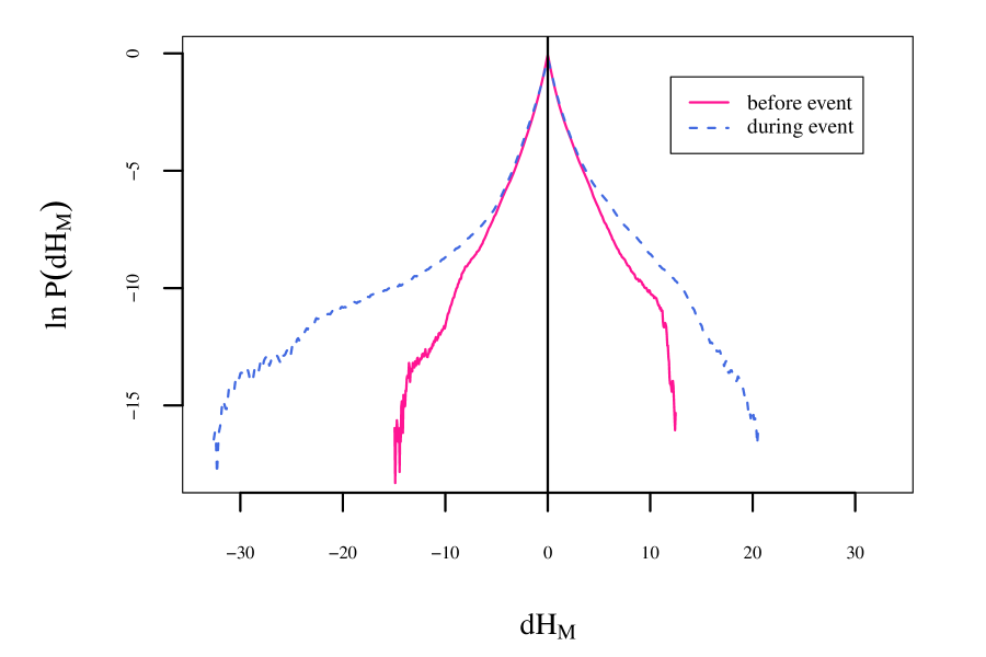
Figure 6: (Above) probability distribution and (below) cumulative distribution of local magnetic helicity, i.e. $dH_{\mathrm{M}}=\mbox{\boldmath$A$}\cdot\mbox{\boldmath$B$}$ in the simulation volume before and during a shear burst event in simulation g1. During this shear burst, as the global magnetic helicity grows, the tail of negative magnetic helicity grows, and grows much higher than the positive tail.

Shear bursts generate significant currents through magnetic shear, which change the global magnetic helicity. When no shear burst is present in the system small filaments of high current are common and likely indicate slow reconnection on small scales. However when a shear burst grows, large-scale high-current structures grow at the same time. A typical growth in current around a shear burst is shown in Fig. 7.

Figure 7: Current-squared in the lowest wavenumbers $k=1,2,3,4$ scaled to its initial time-value during a shear burst in simulation g2. Global current-squared and magnetic shear are shown scaled and shifted to fit on the same scale for reference.

In simulations similar to those discussed in this work, but performed with fully-periodic boundary conditions (sometimes called homogenous Rayleigh Bénard boundary conditions), the macroscopic elevator instability as it is presented by Calzavarini et al. (2006, 2005); Škandera (2007) can be readily identified. The elevator instability is an exact solution to the equations of motion in the homogeneous system. It is an extreme realization of the fact that the homogeneous, incompressible flow can gain vast amounts of energy by coherent large-scale vertical motions. The elevator instability creates parallel, vertical jets ($k_{z}=0$) of alternating direction throughout the volume that significantly degrade the quality of turbulence statistics. The flow pattern created by this elevator instability fully destroys the original, natural flow field. The instability can be eliminated in homogeneous Boussinesq systems by considering a horizontal mean temperature gradient (Škandera & Müller, 2009).

In the quasi-periodic simulations presented in this work, we find no evidence of this instability although we follow the simulations for extremely long times. Mean flows parallel to gravity are manually suppressed in our quasi-periodic set-up. In contrast to the elevator instability, shear bursts are embedded into the turbulence and have limited coherence and lifetime with regard to the full flow-field. Shear bursts do not exhibit exponential growth of energy nor is their growth rate dependent on clear system parameters like the Prandtl number. The shear burst is superficially similar to the elevator instability because both involve coherent flows. However, the coherent flows associated with a shear burst do not display a preference for any fixed spatial direction, but follow a sometimes complicated, curved path in a localized section of the simulation volume. This flow path can change during the evolution of the shear burst, and is different for each shear burst. When the violent elevator instability is present, it is likely to mask finer-scale processes like the shear burst.

4 Conclusions

We have isolated a basic mechanism of dynamo action in MHD convection that operates through spontaneously developing, intermittent bursts of high shear during steady-state dynamo action. Because this process occurs in all simulations considered here, it is of potential importance for astrophysical small-scale dynamo action in turbulent convection scenarios. Shear bursts consist of the formation of coherent, highly-sheared flows along-side magnetic structures with a strong magnetic-helicity polarity bias. The slow growth and eventual decay of the magnetic helicity structure is key to the shear burst phenomenon. The increasing shear causes a gradual rise in energy on all spatial scales due to magnetic stretching in the system over several buoyancy times. After some time, the shear flows lose their alignment and decay. Once the shear flows are destroyed, the elevated energy dissipates over several buoyancy times. Closely spaced shear bursts can occur in a series, creating long periods of time where magnetic energy is elevated significantly above the steady state.