Fractional Non-Linear, Linear and Sublinear Death Processes

Abstract

This paper is devoted to the study of a fractional version of non-linear $\mathpzc{M}^{\nu}(t)$, $t>0$, linear $M^{\nu}(t)$, $t>0$ and sublinear $\mathfrak{M}^{\nu}(t)$, $t>0$ death processes. Fractionality is introduced by replacing the usual integer-order derivative in the difference-differential equations governing the state probabilities, with the fractional derivative understood in the sense of Dzhrbashyan–Caputo. We derive explicitly the state probabilities of the three death processes and examine the related probability generating functions and mean values. A useful subordination relation is also proved, allowing us to express the death processes as compositions of their classical counterparts with the random time process $T_{2\nu}(t)$, $t>0$. This random time has one-dimensional distribution which is the folded solution to a Cauchy problem of the fractional diffusion equation.

1 Introduction

We assume that we have a population of $n_{0}$ individuals or objects. The components of this population might be the set of healthy people during an epidemic or the set of items being sold in a store, or even, say, melting ice pack blocks. However even a coalescence of particles can be treated in this same manner, leading to a large ensemble of physical analogues suited to the method. The main interest is to model the fading process of these objects and, in particular, to analyse how the size of the population decreases.

The classical death process is a model describing this type of phenomena and, its linear version is analysed in bailey, page 90. The most interesting feature of the extinguishing population is the probability distribution

$$p_{k}(t)=\text{Pr}\left\{M(t)=k\mid M(0)=n_{0}\right\},\qquad t>0,\>0\leq k\leq n_{0},$$ (1.1)

where $M(t)$, $t>0$ is the point process representing the size of the population at time $t$. If the death rates are proportional to the population size, the process is called linear and the probabilities (1.1) are solutions to the initial-value problem

$$\begin{cases}\frac{d}{dt}p_{k}(t)=\mu(k+1)p_{k+1}(t)-\mu kp_{k}(t),&0\leq k\leq n_{0},\\ p_{k}(0)=\begin{cases}1,&k=n_{0},\\ 0,&0\leq k<n_{0},\end{cases}\end{cases}$$ (1.2)

with $p_{n_{0}+1}(t)=0$.

The distribution satisfying (1.2) is

$$p_{k}(t)=\binom{n_{0}}{k}e^{-\mu kt}\left(1-e^{-\mu t}\right)^{n_{0}-k},\qquad 0\leq k\leq n_{0}.$$ (1.3)

The equations (1.2) are based on the fact that the death rate of each component of the population is proportional to the number of existing individuals.

In the non-linear case, where the death rates are $\mu_{k}$, $0\leq k\leq n_{0}$, equations (1.2) must be replaced by

$$\begin{cases}\frac{d}{dt}\mathpzc{p}_{k}(t)=\mu_{k+1}\mathpzc{p}_{k+1}(t)-\mu_{k}\mathpzc{p}_{k}(t),&0\leq k\leq n_{0},\\ \mathpzc{p}_{k}(0)=\begin{cases}1,&k=n_{0},\\ 0,&0\leq k<n_{0}.\end{cases}\end{cases}$$ (1.4)

In this paper we consider fractional versions of the processes described above, where fractionality is obtained by substitution of the integer-order derivatives appearing in (1.2) and (1.4), with the fractional derivative called Caputo or Dzhrbashyan–Caputo derivative, defined as follows

$$\begin{cases}\frac{d^{\nu}f\left(t\right)}{dt^{\nu}}=\frac{1}{\Gamma\left(1-\nu\right)}\displaystyle\int_{0}^{t}\frac{f^{\prime}\left(s\right)}{\left(t-s\right)^{\nu}}\,ds,&0<\nu<1,\\ f^{\prime}\left(t\right),&\nu=1.\end{cases}$$ (1.5)

The main advantage of the Dzhrbashyan–Caputo fractional derivative over the usual Riemann–Liouville fractional derivatives is that the former requires only integer-order derivatives in the initial conditions.

The fractional derivative operator is vastly present in the physical and mathematical literature. It appears for example in generalisations of diffusion-type differential equations (see wyss, wyss2, nigmatullin and mainardi), hyperbolic equations such as telegraph equation (see orsbeg), reaction-diffusion equations (see saxena1), or in the study of continuous time random walks (CTRW) scaling limits (see kol1, meer). Fractional calculus has also been considered by some authors to describe cahotic Hamiltonian dynamics in low dimensional systems (see e.g. zas, zas2, saxena2, saxena3 and saxena4). For a complete review of fractional kinetics the reader can consult zas3 or the book by Zaslavsky zas4. In the literature are also present fractional generalisations of point processes, such as the Poisson process (see repin, laskin, scalas, cahoy, sibatov and orsbeg2) and the birth and birth-death processes (see cahoy2, pol, pol2). Fractional models are also used in other fields, for example finance (scalas2, scalas3).

The population size is governed by

$$\begin{cases}\frac{d^{\nu}}{dt^{\nu}}\mathpzc{p}_{k}(t)=\mu_{k+1}\mathpzc{p}_{k+1}(t)-\mu_{k}\mathpzc{p}_{k}(t),&0\leq k\leq n_{0},\\ \mathpzc{p}_{k}^{\nu}(0)=\begin{cases}1,&k=n_{0},\\ 0,&0\leq k<n_{0},\end{cases}\end{cases}$$ (1.6)

and is denoted by $\mathpzc{M}^{\nu}(t)$, $t>0$.

Let us assume that a crack has the form of a process $T_{2\nu}(t)$, $t>0$. For $\nu=1/2$, this coincides with a reflecting Brownian motion and has been described and derived in kunin. For $\nu\neq 1/2$, the process $T_{2\nu}(t)$, $t>0$, can be identified with a stable process (see for details on this point orsbeg3). The ensemble of $n_{0}$ particles moves on the fracture and, at the same time, undergoes a decaying process which respects the same probabilistic rules of the usual death process. For the number of existing particles, we have therefore

$$\mathpzc{p}^{\nu}_{k}(t)=\int_{0}^{\infty}\mathpzc{p}_{k}(s)\text{Pr}\left\{T_{2\nu}(t)\in ds\right\}.$$ (1.7)

We observe that

$$\text{Pr}\left\{T_{2\nu}(t)\in ds\right\}=q(s,t)ds,$$ (1.8)

is a solution to

$$\frac{\partial^{2\nu}}{\partial t^{2\nu}}q(s,t)=\frac{\partial^{2}}{\partial s^{2}}q(s,t),\qquad s>0,\>t>0,$$ (1.9)

with the necessary initial conditions. Furthermore we recall that

$$\int_{0}^{\infty}e^{-zt}q(s,t)dt=z^{\nu-1}e^{-z^{\nu}s},\qquad z>0,\>s>0.$$ (1.10)

The distribution $q(s,t)$ is also a solution to

$$\frac{\partial^{\nu}}{\partial t^{\nu}}q(s,t)=-\frac{\partial}{\partial s}q(s,t),\qquad s>0,$$ (1.11)

as can be ascertained directly. If we take the fractional derivative in (1.7) we get

$$\frac{d^{\nu}}{dt^{\nu}}\mathpzc{p}^{\nu}_{k}(t) =\int_{0}^{\infty}\mathpzc{p}_{k}(s)\frac{\partial^{\nu}}{\partial t^{\nu}}\text{Pr}\left\{T_{2\nu}(t)\in ds\right\}$$ (1.12)

$$=-\int_{0}^{\infty}\mathpzc{p}_{k}(s)\frac{\partial}{\partial s}q(s,t)ds$$

$$=-q(s,t)\mathpzc{p}_{k}(s)\big{|}_{0}^{\infty}+\int_{0}^{\infty}\frac{d\mathpzc{p}_{k}(s)}{ds}q(s,t)ds$$

$$=\int_{0}^{\infty}\left[-\mu_{k}\mathpzc{p}_{k}(s)+\mu_{k+1}\mathpzc{p}_{k+1}(s)\right]q(s,t)ds$$

$$=-\mu_{k}\mathpzc{p}_{k}^{\nu}(t)+\mu_{k+1}\mathpzc{p}^{\nu}_{k+1}(t).$$

This shows that replacing the time derivative with the fractional derivative corresponds to considering a death process (annihilating process) on particles displacing on a crack.

We now give some details about (1.11). By taking the Laplace transform of both members of (1.11) we have that

$$\int_{0}^{\infty}e^{-zt}\frac{\partial^{\nu}}{\partial t^{\nu}}q(s,t)dt =-\frac{\partial}{\partial s}\left(\int_{0}^{\infty}e^{-zt}q(s,t)dt\right)$$ (1.13)

$$=-\frac{\partial}{\partial s}\left(z^{\nu-1}e^{-sz^{\nu}}\right)=z^{2\nu-1}e^{-sz^{\nu}}.$$

Furthermore,

$$\int_{0}^{\infty}e^{-zt}\frac{\partial^{\nu}}{\partial t^{\nu}}q(s,t)dt =z^{\nu}\int_{0}^{\infty}e^{-zt}q(s,t)dt-z^{\nu-1}q(s,0)$$ (1.14)

$$=z^{\nu}\left(z^{\nu-1}e^{-sz^{\nu}}\right)-z^{\nu-1}\delta(s),$$

and therefore for $s>0$ this establishes that $q(s,t)$ solves equation (1.11). We note that a gas particle moving on a fracture has inspired to different authors the iterated Brownian motion (see deblassie).

The distribution

$$\mathpzc{p}_{k}^{\nu}(t)=\text{Pr}\left\{\mathpzc{M}^{\nu}(t)=k\mid\mathpzc{M}^{\nu}(0)=n_{0}\right\},\qquad 0\leq k\leq n_{0},$$ (1.15)

is obtained explicitly and reads

$$\mathpzc{p}_{k}^{\nu}(t)=\begin{cases}E_{\nu,1}(-\mu_{n_{0}}t^{\nu}),&k=n_{0},\\ \textstyle\prod\limits_{j=k+1}^{n_{0}}\mu_{j}\displaystyle\sum_{m=k}^{n_{0}}\frac{E_{\nu,1}(-\mu_{m}t^{\nu})}{\textstyle\prod\limits_{\begin{subarray}{c}h=k\\ h\neq m\end{subarray}}^{n_{0}}\left(\mu_{h}-\mu_{m}\right)},&0<k<n_{0},\\ 1-\displaystyle\sum_{m=1}^{n_{0}}\displaystyle\prod_{\begin{subarray}{c}h=1\\ h\neq m\end{subarray}}^{n_{0}}\left(\frac{\mu_{h}}{\mu_{h}-\mu_{m}}\right)E_{\nu,1}(-\mu_{m}t^{\nu}),&k=0,\>n_{0}>1.\end{cases}$$ (1.16)

Obviously, for $k=0$, $n_{0}=1$,

$$\mathpzc{p}_{0}^{\nu}(t)=1-E_{\nu,1}(-\mu_{1}t^{\nu}).$$ (1.17)

The Mittag-Leffler functions appearing in (1.16) are defined as

$$E_{\nu,\gamma}\left(x\right)=\sum_{h=0}^{\infty}\frac{x^{h}}{\Gamma\left(\nu h+\gamma\right)},\qquad x\in\mathbb{R},\quad\nu,\gamma>0.$$ (1.18)

For $\nu=\gamma=1$, $E_{1,1}(x)=e^{x}$ and formulae (1.16) provide the explicit distribution of the classical non-linear death process.

For $\mu_{k}=k\mu$ the distribution of the fractional linear death process can be obtained either directly by solving the Cauchy problem (1.6) with $\mu_{k}=k\cdot\mu$ and $p_{n_{0}+1}(t)=0$, or by specialising (1.16) resulting in the following form

$$p_{k}^{\nu}(t)=\binom{n_{0}}{k}\sum_{r=0}^{n_{0}-k}\binom{n_{0}-k}{r}(-1)^{r}E_{\nu,1}(-(k+r)\mu t^{\nu}).$$ (1.19)

A technical tool necessary for our manipulations is the Laplace transform of Mittag-Leffler functions which we write here for the sake of completeness:

$$\int_{0}^{\infty}e^{-zt}t^{\gamma-1}E_{\nu,\gamma}(\pm\vartheta t^{\nu})dt=\frac{z^{\nu-\gamma}}{z^{\nu}\mp\vartheta},\qquad\mathfrak{R}(z)>|\vartheta|^{\frac{1}{\nu}}.$$ (1.20)

Another special case is the so-called fractional sublinear death process (for sublinear birth processes consult donnelly) where the death rates have the form $\mu_{k}=\mu(n_{0}+1-k)$. In the sublinear process, the annihilation of particles or individuals accelerates with decreasing population size.

The distribution $\mathfrak{p}_{k}^{\nu}(t)$, $0\leq k\leq n_{0}$ of the fractional sublinear death process $\mathfrak{M}^{\nu}(t)$, $t>0$, is strictly related to that of the fractional linear birth process $N^{\nu}(t)$, $t>0$ (see, for details on this point, pol):

$$\text{Pr}\left\{\mathfrak{M}^{\nu}(t)=0\mid\mathfrak{M}^{\nu}(0)=n_{0}\right\}=\text{Pr}\left\{N^{\nu}(t)>n_{0}\mid N^{\nu}(0)=1\right\}.$$ (1.21)

In general, the connection between the fractional sublinear death process and the fractional linear birth process is expressed by the relation

$$\text{Pr}\left\{\mathfrak{M}^{\nu}(t)=n_{0}-(k-1)\mid\mathfrak{M}^{\nu}(0)=n_{0}\right\}$$ (1.22)

$$=\text{Pr}\left\{N^{\nu}(t)=k\mid N^{\nu}(0)=1\right\},\qquad 1\leq k\leq n_{0}.$$

This shows a sort of symmetry in the evolution of fractional linear birth and fractional sublinear death processes.

For all fractional processes considered in this paper, a subordination relationship holds. In particular, for the fractional linear death process we can write that

$$M^{\nu}(t)=M(T_{2\nu}(t)),\qquad 0<\nu<1,\>t>0,$$ (1.23)

where $T_{2\nu}(t)$ is a process for which

$$\text{Pr}\left\{T_{2\nu}(t)\in ds\right\}=q(s,t)ds,$$ (1.24)

is a solution to the following Cauchy problem (see ob)

$$\begin{cases}\frac{\partial^{2\nu}}{\partial t^{2\nu}}q(s,t)=\frac{\partial^{2}}{\partial s^{2}}q(s,t),&t>0,\>s>0,\\ \left.\frac{\partial}{\partial t}q(s,t)\right|_{s=0}=0,\\ q(s,0)=\delta(s),&0<\nu\leq 1,\end{cases}$$ (1.25)

with the additional initial condition

$$q_{t}(s,0)=0,\qquad 1/2<\nu\leq 1.$$ (1.26)

In equation (1.23), $M(t)$, $t>0$, represents the classical linear death process. Subordination relations of this type are extensively treated in orsbeg3 and koloko.

We also show that all the fractional death processes considered below can be viewed as classical death processes with rate $\mu\cdot\Xi$, where $\Xi$ is a Wright-distributed random variable.

2 The fractional linear death process and its properties

In this section we derive the distribution of the fractional linear death process as well as some interesting related properties and interpretations.

Theorem 1.

The distribution of the fractional linear death process $M^{\nu}(t)$, $t>0$ with $n_{0}$ initial individuals and death rates $\mu_{k}=\mu\cdot k$, is given by

$$p_{k}^{\nu}(t) =\text{Pr}\left\{M^{\nu}(t)=k\mid M^{\nu}(0)=n_{0}\right\}$$ (2.1)

$$=\binom{n_{0}}{k}\sum_{r=0}^{n_{0}-k}\binom{n_{0}-k}{r}(-1)^{r}E_{\nu,1}(-(k+r)\mu t^{\nu}),$$

where $0\leq k\leq n_{0}$, $t>0$ and $\nu\in(0,1]$. The function $E_{\nu,1}(x)$ is the Mittag-Leffler function previously defined in (1.18).

Proof.

The state probability $p_{n_{0}}^{\nu}(t)$, $t>0$ is readily obtained by applying the Laplace transform to equation (1.6), with $\mu_{k}=\mu\cdot k$, and then transforming back the result, thus yielding

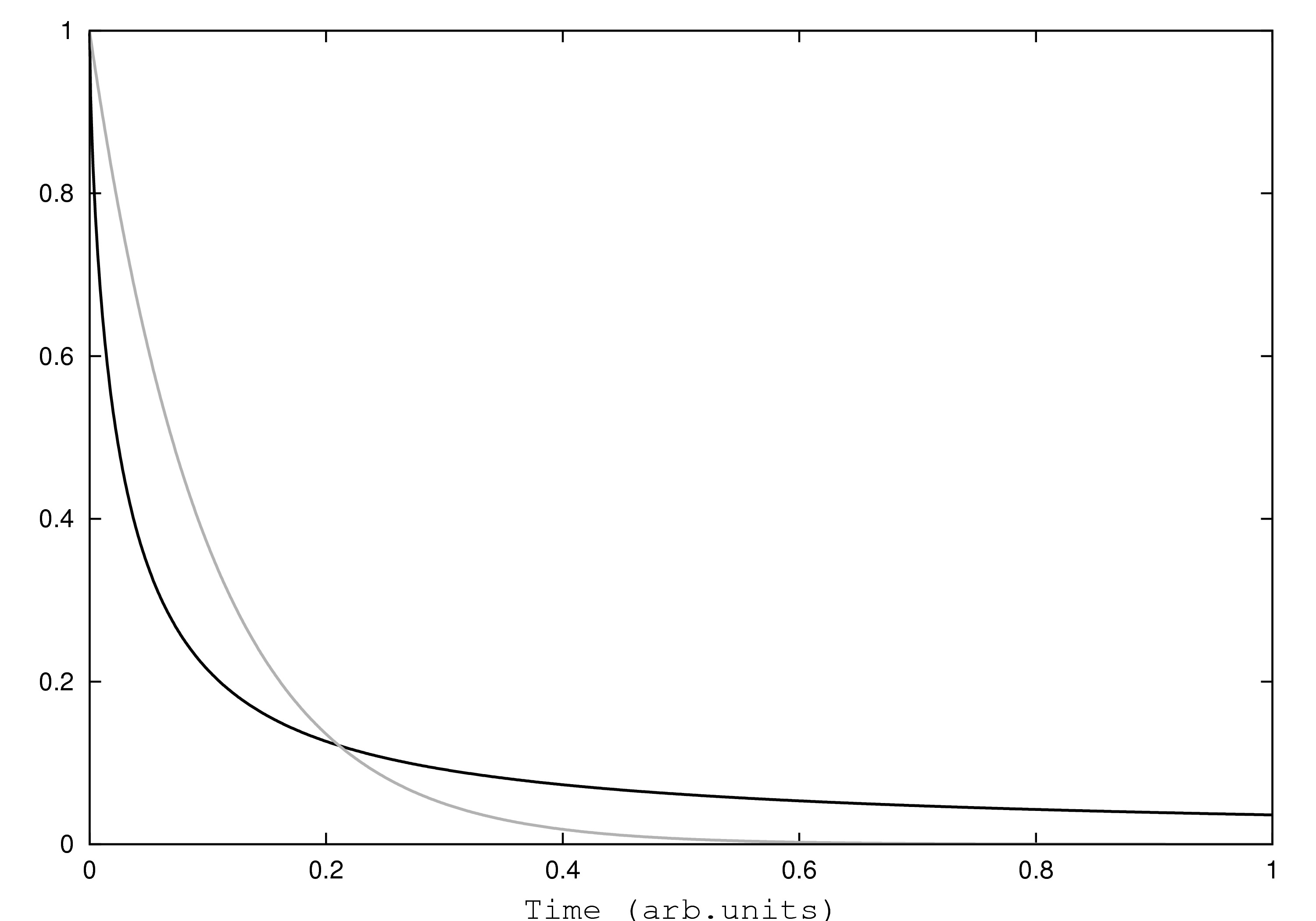
Figure 1: Plot of $p_{n_{0}}^{0.7}(t)$ (in black) and $p_{n_{0}}^{1}(t)$ (in grey), both with $n_{0}=10$.

$$p_{n_{0}}^{\nu}(t)=E_{\nu,1}(-n_{0}\mu t^{\nu}),\qquad t>0,\>\nu\in(0,1].$$ (2.2)

When $k=n_{0}-1$, in order to solve the related differential equation, we can write

$$z^{\nu}\mathcal{L}\left\{p_{n_{0}-1}\right\}(z)=\mu n_{0}\frac{z^{\nu-1}}{z^{\nu}+n_{0}\mu}-\mu(n_{0}-1)\mathcal{L}\left\{p_{n_{0}-1}\right\}(z)$$ (2.3)

$$\Leftrightarrow\quad\mathcal{L}\left\{p_{n_{0}-1}\right\}(z)=\mu n_{0}z^{\nu-1}\frac{1}{z^{\nu}+n_{0}\mu}\cdot\frac{1}{z^{\nu}+(n_{0}-1)\mu}$$

$$\Leftrightarrow\quad\mathcal{L}\left\{p_{n_{0}-1}\right\}(z)=n_{0}z^{\nu-1}\left(\frac{1}{z^{\nu}+(n_{0}+1)\mu}-\frac{1}{z^{\nu}+n_{0}\mu}\right).$$

By inverting equation (2.3), we readily obtain that

$$p_{n_{0}-1}^{\nu}(t)=n_{0}\left(E_{\nu,1}(-(n_{0}-1)\mu t^{\nu})-E_{\nu,1}(-n_{0}\mu t^{\nu})\right).$$ (2.4)

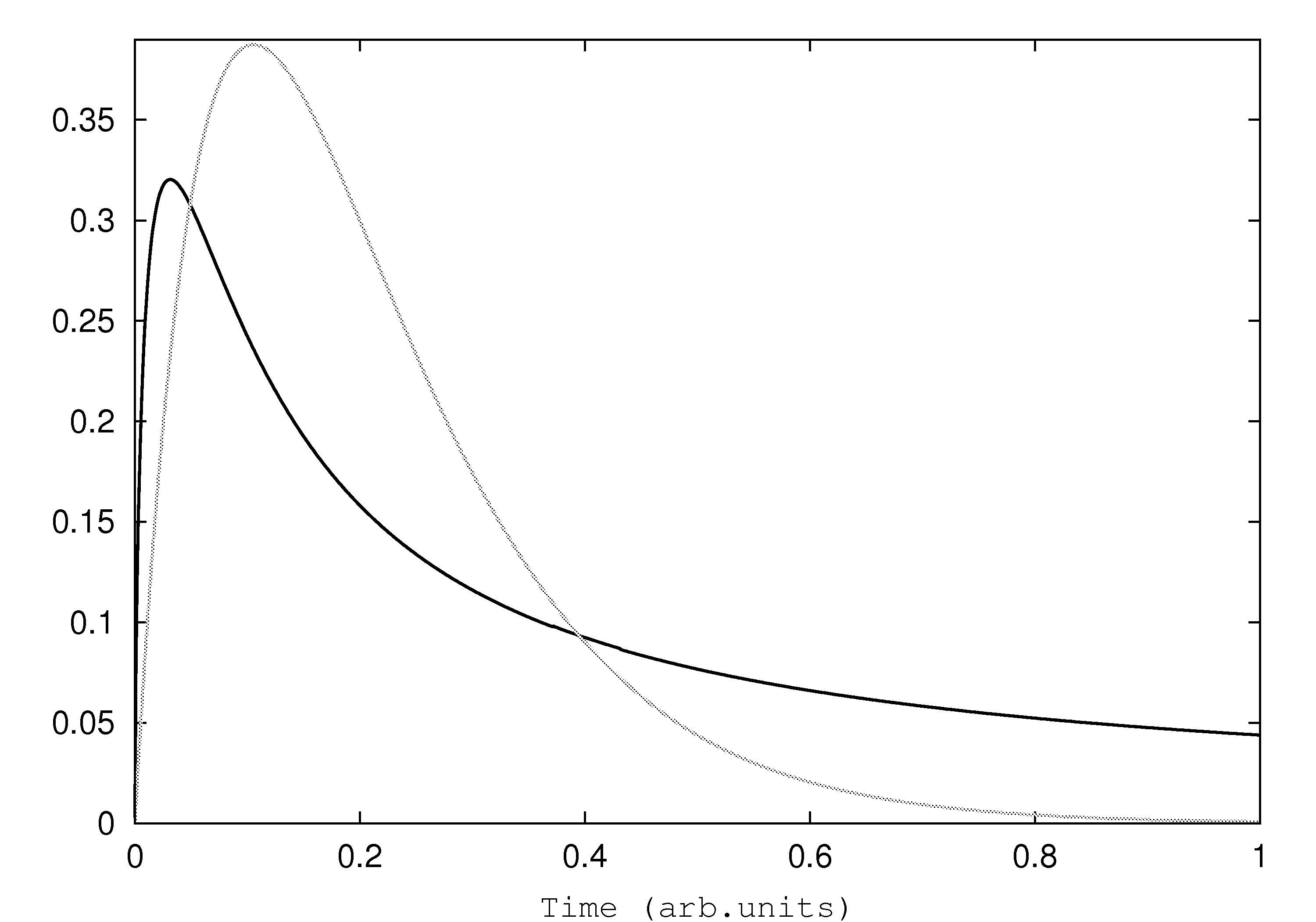
Figure 2: Plot of $p_{n_{0}-1}^{0.7}(t)$ (in black) and $p_{n_{0}-1}^{1}(t)$ (in grey). Here $n_{0}=10$.

For general values of $k$, with $0\leq k<n_{0}$, we must solve the following Cauchy problem:

$$\frac{d^{\nu}}{dt^{\nu}}p_{k}(t) =\mu(k+1)\binom{n_{0}}{k+1}$$ (2.5)

$$\times\sum_{r=0}^{n_{0}-k-1}\binom{n_{0}-k-1}{r}(-1)^{r}E_{\nu,1}(-(k+1+r)\mu t^{\nu})-\mu kp_{k}(t),$$

subject to the initial condition $p_{k}(0)=0$ and with $\nu\in(0,1]$. The solution can be found by resorting to the Laplace transform, as we see in the following.

$$z^{\nu}\mathcal{L}\left\{p_{k}\right\}(z) =\mu(k+1)\binom{n_{0}}{k+1}$$ (2.6)

$$\times\sum_{r=0}^{n_{0}-k-1}\binom{n_{0}-k-1}{r}(-1)^{r}\frac{z^{\nu-1}}{z^{\nu}+(k+1+r)\mu}-\mu k\mathcal{L}\left\{p_{k}\right\}(z).$$

The Laplace transform $\mathcal{L}\left\{p_{k}\right\}(z)$ can thus be written as

$$\mathcal{L}\left\{p_{k}\right\}(z)$$ (2.7)

$$=\mu(k+1)\binom{n_{0}}{k+1}\sum_{r=0}^{n_{0}-k-1}\binom{n_{0}-k-1}{r}(-1)^{r}\frac{z^{\nu-1}}{z^{\nu}+(k+1+r)\mu}\cdot\frac{1}{z^{\nu}+k\mu}$$

$$=\binom{n_{0}}{k}\sum_{r=0}^{n_{0}-k-1}\binom{n_{0}-k}{r+1}(-1)^{r}z^{\nu-1}\left(\frac{1}{z^{\nu}+k\mu}-\frac{1}{z^{\nu}+(k+1+r)\mu}\right)$$

$$=\binom{n_{0}}{k}\sum_{j=1}^{n_{0}-k}\binom{n_{0}-k}{j}(-1)^{j-1}z^{\nu-1}\left(\frac{1}{z^{\nu}+k\mu}-\frac{1}{z^{\nu}+(k+j)\mu}\right)$$

$$=\binom{n_{0}}{k}\sum_{j=1}^{n_{0}-k}\binom{n_{0}-k}{j}(-1)^{j}\frac{z^{\nu-1}}{z^{\nu}+(k+j)\mu}$$

$$\qquad-\binom{n_{0}}{k}\frac{z^{\nu-1}}{z^{\nu}+k\mu}\sum_{j=1}^{n_{0}-k}\binom{n_{0}-k}{j}(-1)^{j}$$

$$=\binom{n_{0}}{k}\sum_{j=1}^{n_{0}-k}\binom{n_{0}-k}{j}(-1)^{j}\frac{z^{\nu-1}}{z^{\nu}+(k+j)\mu}+\binom{n_{0}}{k}\frac{z^{\nu-1}}{z^{\nu}+k\mu}$$

$$=\binom{n_{0}}{k}\sum_{j=0}^{n_{0}-k}\binom{n_{0}-k}{j}(-1)^{j}\frac{z^{\nu-1}}{z^{\nu}+(k+j)\mu}.$$

∎

By taking now the inverse Laplace transform of (2.7), we obtain the claimed result (1.19).

Remark 1.

When $\nu=1$, equation (1.19) easily reduces to the distribution of the classical linear death process, i.e.

$$p_{k}(t)=\binom{n_{0}}{k}e^{-k\mu t}\left(1-e^{-\mu t}\right)^{n_{0}-k},\qquad t>0,\>0\leq k\leq n_{0}.$$ (2.8)

In the following theorem we give a proof of an interesting subordination relation.

Theorem 2.

The fractional linear death process $M^{\nu}(t)$, $t>0$ can be represented as

$$M^{\nu}(t)\overset{i.d.}{=}M(T_{2\nu}(t)),\qquad t>0,\>\nu\in(0,1],$$ (2.9)

where $M(t)$, $t>0$ is the classical linear death process (see e.g. bailey, page 90) and $T_{2\nu}(t)$, $t>0$, is a random time process whose one-dimensional distribution coincides with the folded solution to the following fractional diffusion equation

$$\begin{cases}\frac{\partial^{2\nu}}{\partial t^{2\nu}}q(s,t)=\frac{\partial^{2}}{\partial s^{2}}q(s,t),&t>0,\>\nu\in(0,1],\\ q(s,0)=\delta(s),\end{cases}$$ (2.10)

with the additional condition $q_{t}(s,0)=0$ if $\nu\in(1/2,1]$ (see ob).

Proof.

By evaluating the Laplace transform of the generating function of the fractional linear death process $M^{\nu}(t)$, $t>0$, we obtain that

$$\int_{0}^{\infty}e^{-zt}G^{\nu}(u,t)dt$$ (2.11)

$$=\int_{0}^{\infty}e^{-zt}\sum_{k=0}^{n_{0}}u^{k}\binom{n_{0}}{k}\sum_{r=0}^{n_{0}-k}\binom{n_{0}-k}{r}(-1)^{r}E_{\nu,1}(-(k+r)\mu t^{\nu})dt$$

$$=\sum_{0}^{n_{0}}u^{k}\binom{n_{0}}{k}\sum_{r=0}^{n_{0}-k}\binom{n_{0}-k}{r}(-1)^{r}\frac{z^{\nu-1}}{z^{\nu}+(k+r)\mu}$$

$$=\int_{0}^{\infty}\sum_{k=0}^{n_{0}}u^{k}\binom{n_{0}}{k}\sum_{r=0}^{n_{0}-k}\binom{n_{0}-k}{r}(-1)^{r}z^{\nu-1}e^{-s(z^{\nu}+(k+r)\mu)}ds$$

$$=\int_{0}^{\infty}e^{-sz^{\nu}}z^{\nu-1}\left\{\sum_{k=0}^{n_{0}}u^{k}\binom{n_{0}}{k}\sum_{r=0}^{n_{0}-k}\binom{n_{0}-k}{r}(-1)^{r}e^{-s(k+r)\mu}\right\}ds$$

$$=\int_{0}^{\infty}e^{-sz^{\nu}}z^{\nu-1}\left\{\sum_{k=0}^{n_{0}}u^{k}\binom{n_{0}}{k}e^{-\mu sk}\sum_{r=0}^{n_{0}-k}\binom{n_{0}-k}{r}(-1)^{r}e^{-sr\mu}\right\}ds$$

$$=\int_{0}^{\infty}e^{-sz^{\nu}}z^{\nu-1}\left\{\sum_{k=0}^{n_{0}}u^{k}\binom{n_{0}}{k}e^{-\mu sk}(1-e^{-\mu s})^{n_{0}-k}\right\}ds$$

$$=\int_{0}^{\infty}e^{-sz^{\nu}}z^{\nu-1}G(u,s)ds$$

$$=\int_{0}^{\infty}e^{-zt}\int_{0}^{\infty}\sum_{k=0}^{n_{0}}u^{k}\text{Pr}\left\{M(s)=k\right\}f_{T_{2\nu}}(s,t)ds\,dt$$

$$=\int_{0}^{\infty}e^{-zt}\left\{\sum_{k=0}^{\infty}u^{k}\text{Pr}\left\{M(T_{2\nu}(t))=k\right\}\right\}dt,$$

and this is sufficient to prove that (2.9) holds. Note that we used two facts. The first one is that

$$\int_{0}^{\infty}e^{-zt}f_{T_{2\nu}}(s,t)dt=z^{\nu-1}e^{-sz^{\nu}},\qquad s>0,\>z>0,$$ (2.12)

is the Laplace transform of the solution to (2.10). The second fact is that the Laplace transform of the Mittag-Leffler function is

$$\int_{0}^{\infty}e^{-zt}E_{\nu,1}(-\vartheta t^{\nu})dt=\frac{z^{\nu-1}}{z^{\nu}+\vartheta}.$$ (2.13)

∎

In figures 1 and 2, we compare the behaviour of the fractional probabilities $p_{n_{0}}^{0.7}(t)$ and $p_{n_{0}-1}^{0.7}(t)$ with their classical counterparts $p_{n_{0}}^{1}(t)$ and $p_{n_{0}-1}^{1}(t)$, $t>0$. What emerges from the inspection of both figures is that, for large values of $t$, the probabilities, in the fractional case, decrease more slowly than $p_{n_{0}}^{1}(t)$ and $p_{n_{0}-1}^{1}(t)$. The probability $p_{n_{0}-1}^{0.7}(t)$, increases initially faster than $p_{n_{0}-1}^{1}(t)$, but after a certain time lapse, $p_{n_{0}-1}^{1}(t)$ dominates $p_{n_{0}-1}^{0.7}(t)$.

Remark 2.

For $\nu=1/2$, in view of the integral representation

$$E_{\frac{1}{2},1}(x)=\frac{2}{\sqrt{\pi}}\int_{0}^{\infty}e^{-w^{2}+2xw}dw,\qquad x\in\mathbb{R},$$ (2.14)

we extract from (1.19) that

$$p_{k}^{\frac{1}{2}}(t) =\frac{2}{\sqrt{\pi}}\int_{0}^{\infty}e^{-w^{2}}\binom{n_{0}}{k}\sum_{r=0}^{n_{0}-k}\binom{n_{0}-k}{r}(-1)^{r}e^{-2w(k+r)\mu t^{\frac{1}{2}}}$$ (2.15)

$$=\int_{0}^{\infty}\frac{e^{-\frac{y^{2}}{4t}}}{\sqrt{\pi t}}p_{k}^{1}(y)dy=\text{Pr}\left\{M(\left|B(t)\right|)=k\right\},$$

where $B(t)$, $t>0$ is a Brownian motion with volatility equal to 2.

Remark 3.

We can interpret formula (1.19) in an alternative way, as follows. For each integer $k\in[0,n_{0}]$ we have that

$$p_{k}^{\nu}(t) =\text{Pr}\left\{M^{\nu}(t)=k\mid M^{\nu}(0)=n_{0}\right\}$$ (2.16)

$$=\int_{0}^{\infty}p_{k}(s)\text{Pr}\left\{T_{2\nu}(t)\in ds\right\}$$

$$=\binom{n_{0}}{k}\sum_{r=0}^{n_{0}-k}\binom{n_{0}-k}{r}(-1)^{r}\int_{0}^{\infty}e^{-\mu(k+r)s}\text{Pr}\left\{T_{2\nu}(t)\in ds\right\}$$

$$=\binom{n_{0}}{k}\sum_{r=0}^{n_{0}-k}\binom{n_{0}-k}{r}(-1)^{r}\int_{0}^{\infty}e^{-\mu(k+r)s}t^{-\nu}W_{-\nu,1-\nu}(-st^{-\nu})ds$$

$$=\binom{n_{0}}{k}\sum_{r=0}^{n_{0}-k}\binom{n_{0}-k}{r}(-1)^{r}\int_{0}^{\infty}e^{-\xi\mu(k+r)t^{\nu}}W_{-\nu,1-\nu}(-\xi)d\xi$$

$$=\int_{0}^{\infty}W_{-\nu,1-\nu}(-\xi)\text{Pr}\left\{M_{\xi}(t^{\nu})=k\mid M_{\xi}(0)=n_{0}\right\}d\xi,$$

where $W_{-\nu,1-\nu}(-\xi)$ is the Wright function defined as

$$W_{-\nu,1-\nu}(-\xi)=\sum_{r=0}^{\infty}\frac{(-\xi)^{r}}{r!\Gamma\left(1-\nu(r+1)\right)},\qquad 0<\nu\leq 1.$$ (2.17)

We therefore obtain an interpretation in terms of a classical linear death process $M_{\Xi}(t)$, $t>0$ evaluated on a new time scale and with random rate $\mu\cdot\Xi$, where $\Xi$ is a random variable, $\xi\in\mathbb{R}^{+}$, with Wright density

$$f_{\Xi}(\xi)=W_{-\nu,1-\nu}(-\xi),\qquad\xi\in\mathbb{R}^{+}.$$ (2.18)

From equation (1.6) with $\mu_{k}=k\cdot\mu$, the related fractional differential equation governing the probability generating function, can be easily obtained, leading to

$$\begin{cases}\frac{\partial^{\nu}}{\partial t^{\nu}}G^{\nu}(u,t)=-\mu u(u-1)\frac{\partial}{\partial u}G^{\nu}(u,t),&\nu\in(0,1],\\ G^{\nu}(u,0)=u^{n_{0}}.\end{cases}$$ (2.19)

From this, and by considering that $\mathbb{E}M^{\nu}(t)=\left.\frac{\partial}{\partial u}G^{\nu}(u,t)\right|_{u=1}$, we obtain that

$$\begin{cases}\frac{d^{\nu}}{dt^{\nu}}\mathbb{E}M^{\nu}(t)=-\mu\mathbb{E}M^{\nu}(t),&\nu\in(0,1],\\ \mathbb{E}M^{\nu}(t)=n_{0}.\end{cases}$$ (2.20)

Equation (2.20) is easily solved by means of the Laplace transforms, yielding

$$\mathbb{E}M^{\nu}(t)=n_{0}E_{\nu,1}(-\mu t^{\nu}),\qquad t>0,\>\nu\in(0,1].$$ (2.21)

Remark 4.

The mean value $\mathbb{E}M^{\nu}(t)$ can also be directly calculated.

$$\mathbb{E}M^{\nu}(t) =\sum_{k=0}^{n_{0}}kp_{k}^{\nu}(t)$$ (2.22)

$$=\sum_{k=0}^{n_{0}}k\binom{n_{0}}{k}\sum_{r=k}^{n_{0}}\binom{n_{0}-k}{r-k}(-1)^{r-k}E_{\nu,1}(-r\mu t^{\nu})$$

$$=\sum_{r=0}^{n_{0}}E_{\nu,1}(-r\mu t^{\nu})(-1)^{r}\sum_{k=1}^{r}k\binom{n_{0}}{k}\binom{n_{0}-k}{r-k}(-1)^{k}$$

$$=\sum_{r=1}^{n_{0}}E_{\nu,1}(-r\mu t^{\nu})(-1)^{r}n_{0}\binom{n_{0}-1}{r-1}\sum_{k=1}^{r}\binom{r-1}{k-1}(-1)^{k}$$

$$=n_{0}E_{\nu,1}(-\mu t^{\nu}).$$

This last step in (2.22) holds because

$$\sum_{k=1}^{r}\binom{r-1}{k-1}(-1)^{k}=\sum_{k=0}^{r-1}\binom{r-1}{k}(-1)^{k+1}=\begin{cases}-1,&r=1,\\ 0,&r>1.\end{cases}$$ (2.23)

3 Related models

In this section we present two models which are related to the fractional linear death process. The first one is its natural generalisation to the non-linear case i.e. we consider death rates in the form $\mu_{k}>0$, $0\leq k\leq n_{0}$. The second one is a sublinear process (see donnelly), namely with death rates in the form $\mu_{k}=\mu(n_{0}+1-k)$; the death rates are thus an increasing sequence as the number of individuals in the population decreases towards zero.

3.1 Generalisation to the non-linear case

Let us denote by $\mathpzc{M}^{\nu}(t)$, $t>0$ the random number of components of a non-linear fractional death process with death rates $\mu_{k}>0$, $0\leq k\leq n_{0}$.

The state probabilities $\mathpzc{p}_{k}^{\nu}(t)=\text{Pr}\left\{\mathpzc{M}^{\nu}(t)=k\mid\mathpzc{M}^{\nu}(0)=n_{0}\right\}$, $t>0$, $0\leq k\leq n_{0}$, $\nu\in(0,1]$ are governed by the following difference-differential equations

$$\begin{cases}\frac{d^{\nu}}{dt^{\nu}}\mathpzc{p}_{k}(t)=\mu_{k+1}\mathpzc{p}_{k+1}(t)-\mu_{k}\mathpzc{p}_{k}(t),&0<k<n_{0},\\ \frac{d^{\nu}}{dt^{\nu}}\mathpzc{p}_{0}(t)=\mu_{1}\mathpzc{p}_{1}(t),&k=0,\\ \frac{d^{\nu}}{dt^{\nu}}\mathpzc{p}_{n_{0}}(t)=-\mu_{n_{0}}\mathpzc{p}_{n_{0}}(t),&k=n_{0},\\ \mathpzc{p}_{k}(0)=\begin{cases}0,&0\leq k<n_{0},\\ 1,&k=n_{0}.\end{cases}\end{cases}$$ (3.1)

The fractional derivatives appearing in (3.1) provide the system with a global memory; i.e. the evolution of the state probabilities $\mathpzc{p}_{k}^{\nu}(t)$, $t>0$, is influenced by the past, as definition (1.5) shows. This is a major difference with the classical non-linear (and, of course, linear and sublinear) death processes, and reverberates in the slowly decaying structure of probabilities extracted from (3.1).

In the non-linear process, the dependence of death rates from the size of the population is arbitrary, and this explains the complicated structure of the probabilities obtained. Further generalisation can be considered by assuming that the death rates depend on $t$ (non-homogeneous, non-linear death process).

We outline here the evaluation of the probabilities $\mathpzc{p}_{k}^{\nu}(t)$, $t>0$, $0\leq k\leq n_{0}$, which can be obtained, as in the linear case, by means of a recursive procedure (similar to that implemented in pol for the fractional linear birth process).

Let $k=n_{0}$. By means of the Laplace transform applied to equation (3.1) we immediately obtain that

$$\mathpzc{p}_{n_{0}}^{\nu}(t)=E_{\nu,1}(-\mu_{n_{0}}t^{\nu}).$$ (3.2)

When $k=n_{0}-1$ we get

$$z^{\nu}\mathcal{L}\left\{\mathpzc{p}_{n_{0}-1}^{\nu}\right\}(z)=-\mu_{n_{0}-1}\mathcal{L}\left\{\mathpzc{p}_{n_{0}-1}^{\nu}\right\}(z)+\mu_{n_{0}}\frac{z^{\nu-1}}{z^{\nu}+\mu_{n_{0}}}$$ (3.3)

$$\Leftrightarrow\mathcal{L}\left\{\mathpzc{p}_{n_{0}-1}^{\nu}\right\}(z)=\mu_{n_{0}}\frac{z^{\nu-1}}{z^{\nu}+\mu_{n_{0}}}\cdot\frac{1}{z^{\nu}+\mu_{n_{0}-1}}$$

$$\Leftrightarrow\mathcal{L}\left\{\mathpzc{p}_{n_{0}-1}^{\nu}\right\}(z)=\mu_{n_{0}}z^{\nu-1}\left[\frac{1}{z^{\nu}+\mu_{n_{0}}}-\frac{1}{z^{\nu}+\mu_{n_{0}-1}}\right]\frac{1}{\mu_{n_{0}-1}-\mu_{n_{0}}}$$

$$\Leftrightarrow\mathpzc{p}_{n_{0}-1}^{\nu}(t)=\frac{\mu_{n_{0}}}{\mu_{n_{0}-1}-\mu_{n_{0}}}\bigg{\{}E_{\nu,1}(-\mu_{n_{0}}t^{\nu})-E_{\nu,1}(-\mu_{n_{0}-1}t^{\nu})\bigg{\}}.$$

For $k=n_{0}-2$ we obtain in the same way that

$$z^{\nu}\mathcal{L}\left\{\mathpzc{p}_{n_{0}-2}^{\nu}\right\}(z)$$ (3.4)

$$=-\mu_{n_{0}-2}\mathcal{L}\left\{\mathpzc{p}_{n_{0}-2}^{\nu}\right\}(z)+\frac{\mu_{n_{0}}\mu_{n_{0}-1}}{\mu_{n_{0}-1}-\mu_{n_{0}}}\left[\frac{z^{\nu-1}}{z^{\nu}+\mu_{n_{0}}}-\frac{z^{\nu-1}}{z^{\nu}+\mu_{n_{0}-1}}\right],$$

so that

$$\mathcal{L}\left\{\mathpzc{p}_{n_{0}-2}^{\nu}\right\}(z)$$ (3.5)

$$={} \frac{\mu_{n_{0}}\mu_{n_{0}-1}}{\mu_{n_{0}-1}-\mu_{n_{0}}}z^{\nu-1}\left[\frac{1}{z^{\nu}+\mu_{n_{0}}}-\frac{1}{z^{\nu}+\mu_{n_{0}-1}}\right]\frac{1}{z^{\nu}+\mu_{n_{0}-2}}$$

$$={} \frac{\mu_{n_{0}}\mu_{n_{0}-1}}{\mu_{n_{0}-1}-\mu_{n_{0}}}z^{\nu-1}\left[\left(\frac{1}{z^{\nu}+\mu_{n_{0}}}-\frac{1}{z^{\nu}+\mu_{n_{0}-2}}\right)\frac{1}{\mu_{n_{0}-2}-\mu_{n_{0}}}\right.$$

$$\left.-\left(\frac{1}{z^{\nu}+\mu_{n_{0}-1}}-\frac{1}{z^{\nu}+\mu_{n_{0}-2}}\right)\frac{1}{\mu_{n_{0}-2}-\mu_{n_{0}-1}}\right].$$

By inverting the Laplace transform we readily arrive at the following result

$$\mathpzc{p}_{n_{0}-2}^{\nu}{} (t)=\mu_{n_{0}}\mu_{n_{0}-1}\left[\frac{E_{\nu,1}(-\mu_{n_{0}}t^{\nu})}{(\mu_{n_{0}-1}-\mu_{n_{0}})(\mu_{n_{0}-2}-\mu_{n_{0}})}\right.$$ (3.6)

$$-\frac{E_{\nu,1}(-\mu_{n_{0}-2}t^{\nu})}{(\mu_{n_{0}-1}-\mu_{n_{0}})(\mu_{n_{0}-2}-\mu_{n_{0}})}-\frac{E_{\nu,1}(-\mu_{n_{0}-1}t^{\nu})}{(\mu_{n_{0}-1}-\mu_{n_{0}})(\mu_{n_{0}-2}-\mu_{n_{0}-1})}$$

$$\left.+\frac{E_{\nu,1}(-\mu_{n_{0}-2}t^{\nu})}{(\mu_{n_{0}-1}-\mu_{n_{0}})(\mu_{n_{0}-2}-\mu_{n_{0}-1})}\right]$$

$$={} \mu_{n_{0}}\mu_{n_{0}-1}\left[\frac{E_{\nu,1}(-\mu_{n_{0}}t^{\nu})}{(\mu_{n_{0}-1}-\mu_{n_{0}})(\mu_{n_{0}-2}-\mu_{n_{0}})}\right.$$

$$+\frac{E_{\nu,1}(-\mu_{n_{0}-2}t^{\nu})}{(\mu_{n_{0}-1}-\mu_{n_{0}})}\left(\frac{1}{\mu_{n_{0}-2}-\mu_{n_{0}-1}}-\frac{1}{\mu_{n_{0}-2}-\mu_{n_{0}}}\right)$$

$$\left.-\frac{E_{\nu,1}(-\mu_{n_{0}-1}t^{\nu})}{(\mu_{n_{0}-1}-\mu_{n_{0}})(\mu_{n_{0}-2}-\mu_{n_{0}-1})}\right]$$

$$={} \mu_{n_{0}}\mu_{n_{0}-1}\left[\frac{E_{\nu,1}(-\mu_{n_{0}}t^{\nu})}{(\mu_{n_{0}-1}-\mu_{n_{0}})(\mu_{n_{0}-2}-\mu_{n_{0}})}\right.$$

$$\left.+\frac{E_{\nu,1}(-\mu_{n_{0}-2}t^{\nu})}{(\mu_{n_{0}-2}-\mu_{n_{0}-1})(\mu_{n_{0}-2}-\mu_{n_{0}})}-\frac{E_{\nu,1}(-\mu_{n_{0}-1}t^{\nu})}{(\mu_{n_{0}-1}-\mu_{n_{0}})(\mu_{n_{0}-2}-\mu_{n_{0}-1})}\right].$$

The structure of the state probabilities for arbitrary values of $k=n_{0}-l$, $0\leq l<n_{0}$, can now be easily obtained. The proof follows the lines of the derivation of the state probabilities for the fractional non-linear pure birth process adopted in Theorem 2.1 in pol. We have that

$$\mathpzc{p}_{n_{0}-l}^{\nu}(t)=\begin{cases}\textstyle\prod\limits_{j=0}^{l-1}\mu_{n_{0}-j}\displaystyle\sum_{m=0}^{l}\frac{E_{\nu,1}(-\mu_{n_{0}-m}t^{\nu})}{\textstyle\prod\limits_{\begin{subarray}{c}h=0\\ h\neq m\end{subarray}}^{l}\left(\mu_{n_{0}-h}-\mu_{n_{0}-m}\right)},&1\leq l<n_{0},\\ E_{\nu,1}(-\mu_{n_{0}}t^{\nu}),&l=0.\end{cases}$$ (3.7)

By means of some changes of indices, formula (3.7) can also be written as

$$\mathpzc{p}_{k}^{\nu}(t)=\begin{cases}\textstyle\prod\limits_{j=k+1}^{n_{0}}\mu_{j}\displaystyle\sum_{m=k}^{n_{0}}\frac{E_{\nu,1}(-\mu_{m}t^{\nu})}{\textstyle\prod\limits_{\begin{subarray}{c}h=k\\ h\neq m\end{subarray}}^{n_{0}}\left(\mu_{h}-\mu_{m}\right)},&0<k<n_{0},\\ E_{\nu,1}(-\mu_{n_{0}}t^{\nu}),&k=n_{0}.\end{cases}$$ (3.8)

For the extinction probability, we have to solve the following initial value problem:

$$\begin{cases}\frac{d^{\nu}}{dt^{\nu}}\mathpzc{p}_{0}(t)=\mu_{1}\textstyle\prod\limits_{j=2}^{n_{0}}\mu_{j}\displaystyle\sum_{m=1}^{n_{0}}\frac{E_{\nu,1}(-\mu_{m}t^{\nu})}{\textstyle\prod\limits_{\begin{subarray}{c}h=1\\ h\neq m\end{subarray}}^{n_{0}}\left(\mu_{h}-\mu_{m}\right)},&n_{0}>1,\\ \frac{d^{\nu}}{dt^{\nu}}\mathpzc{p}_{0}(t)=\mu_{1}E_{\nu,1}(-\mu_{1}t^{\nu}),&n_{0}=1,\\ \mathpzc{p}_{0}(0)=0,&n_{0}\geq 1.\end{cases}$$ (3.9)

When $n_{0}>1$, starting from (3.9) and by resorting to the Laplace transform once again, we have that

$$\mathcal{L}\left\{\mathpzc{p}_{0}^{\nu}\right\}(z)=\textstyle\prod\limits_{j=1}^{n_{0}}\mu_{j}\displaystyle\sum_{m=1}^{n_{0}}\frac{1}{\textstyle\prod\limits_{\begin{subarray}{c}h=1\\ h\neq m\end{subarray}}^{n_{0}}\left(\mu_{h}-\mu_{m}\right)}\cdot\frac{z^{-1}}{z^{\nu}+\mu_{m}}.$$ (3.10)

The inverse Laplace transform of (3.10) leads to

$$\mathpzc{p}_{0}^{\nu}(t) =\textstyle\prod\limits_{j=1}^{n_{0}}\mu_{j}\displaystyle\sum_{m=1}^{n_{0}}\frac{1}{\textstyle\prod\limits_{\begin{subarray}{c}h=1\\ h\neq m\end{subarray}}^{n_{0}}\left(\mu_{h}-\mu_{m}\right)}t^{\nu}E_{\nu,\nu+1}(-\mu_{m}t^{\nu})$$ (3.11)

$$=\textstyle\prod\limits_{j=1}^{n_{0}}\mu_{j}\displaystyle\sum_{m=1}^{n_{0}}\frac{1}{\textstyle\prod\limits_{\begin{subarray}{c}h=1\\ h\neq m\end{subarray}}^{n_{0}}\left(\mu_{h}-\mu_{m}\right)}\cdot\frac{1}{\mu_{m}}\left[1-E_{\nu,1}(-\mu_{m}t^{\nu})\right]$$

$$=\sum_{m=1}^{n_{0}}\prod_{\begin{subarray}{c}h=1\\ h\neq m\end{subarray}}^{n_{0}}\left(\frac{\mu_{h}}{\mu_{h}-\mu_{m}}\right)-\sum_{m=1}^{n_{0}}\prod_{\begin{subarray}{c}h=1\\ h\neq m\end{subarray}}^{n_{0}}\left(\frac{\mu_{h}}{\mu_{h}-\mu_{m}}\right)E_{\nu,1}(-\mu_{m}t^{\nu})$$

$$=1-\sum_{m=1}^{n_{0}}\prod_{\begin{subarray}{c}h=1\\ h\neq m\end{subarray}}^{n_{0}}\left(\frac{\mu_{h}}{\mu_{h}-\mu_{m}}\right)E_{\nu,1}(-\mu_{m}t^{\nu}).$$

Note that, in the last step, we used the following fact:

$$\sum_{m=1}^{n_{0}}\prod_{\begin{subarray}{c}h=1\\ h\neq m\end{subarray}}^{n_{0}}\left(\frac{\mu_{h}}{\mu_{h}-\mu_{m}}\right)=1.$$ (3.12)

This can be ascertained by observing that

$$\prod_{1\leq h<l\leq n_{0}}(\mu_{h}-\mu_{l})=\det\bm{A}=\sum_{j=1}^{n_{0}}a_{1,j}(-1)^{j+1}\text{Min}_{1,j}$$ (3.13)

where

$$\bm{A}=\left|\begin{array}[]{cccc}1&1&\dots&1\\ \mu_{1}&\mu_{2}&\dots&\mu_{n_{0}}\\ \mu_{1}^{2}&\mu_{2}^{2}&\dots&\mu_{n_{0}}^{2}\\ \vdots&\vdots&\ddots&\vdots\\ \mu_{1}^{n_{0}-1}&\mu_{2}^{n_{0}-1}&\dots&\mu_{n_{0}}^{n_{0}-1}\end{array}\right|,$$ (3.14)

is a Vandermonde matrix and $\text{Min}_{1,j}$ is the determinant of the matrix resulting from $\bm{A}$ by removing the first row and the $j$-th column.

When $n_{0}=1$ we obtain

$$\mathcal{L}\left\{\mathpzc{p}_{0}^{\nu}\right\}(z)=\mu_{1}\frac{z^{-1}}{z^{\nu}+\mu_{1}},$$ (3.15)

so that the inverse Laplace transform can be written as

$$\mathpzc{p}_{0}^{\nu}(t) =\mu_{1}t^{\nu}E_{\nu,\nu+1}(-\mu_{1}t^{\nu})$$ (3.16)

$$=1-E_{\nu,1}(-\mu_{1}t^{\nu}).$$

We can therefore summarise the results obtained as follows:

$$\mathpzc{p}_{k}^{\nu}(t)=\begin{cases}{}\textstyle\prod\limits_{j=k+1}^{n_{0}}\mu_{j}\displaystyle\sum_{m=k}^{n_{0}}\frac{E_{\nu,1}(-\mu_{m}t^{\nu})}{\textstyle\prod\limits_{\begin{subarray}{c}h=k\\ h\neq m\end{subarray}}^{n_{0}}\left(\mu_{h}-\mu_{m}\right)},&0<k<n_{0},\>n_{0}>1,\\ E_{\nu,1}(-\mu_{n_{0}}t^{\nu}),&k=n_{0},\>n_{0}\geq 1,\end{cases}$$ (3.17)

and

$$\mathpzc{p}_{0}^{\nu}(t)=\begin{cases}1-\displaystyle\sum_{m=1}^{n_{0}}\displaystyle\prod_{\begin{subarray}{c}h=1\\ h\neq m\end{subarray}}^{n_{0}}\left(\frac{\mu_{h}}{\mu_{h}-\mu_{m}}\right)E_{\nu,1}(-\mu_{m}t^{\nu}),&n_{0}>1,\\ 1-E_{\nu,1}(-\mu_{1}t^{\nu}),&n_{0}=1.\end{cases}$$ (3.18)

3.2 A fractional sublinear death process

We consider in this section the process where the infinitesimal death probabilities have the form

$$\text{Pr}\left\{\mathfrak{M}(t,t+dt]=-1\mid\mathfrak{M}(t)=k\right\}=\mu(n_{0}+1-k)dt+o(dt),$$ (3.19)

where $n_{0}$ is the initial number of individuals in the population. The state probabilities

$$\mathfrak{p}_{k}(t)=\text{Pr}\left\{\mathfrak{M}(t)=k\mid\mathfrak{M}(0)=n_{0}\right\},\qquad 0\leq k\leq n_{0},$$ (3.20)

satisfy the equations

$$\begin{cases}\frac{d}{dt}\mathfrak{p}_{k}(t)=-\mu(n_{0}+1-k)\mathfrak{p}_{k}(t)+\mu(n_{0}-k)\mathfrak{p}_{k+1}(t),&1\leq k\leq n_{0},\\ \frac{d}{dt}\mathfrak{p}_{0}(t)=\mu n_{0}\mathfrak{p}_{1}(t),&k=0,\\ \mathfrak{p}_{k}(0)=\begin{cases}1,&k=n_{0},\\ 0,&0\leq k<n_{0}.\end{cases}\end{cases}$$ (3.21)

In this model the death rate increases with decreasing population size.

The probabilities $\mathfrak{p}_{k}^{\nu}(t)=\text{Pr}\left\{\mathfrak{M}^{\nu}(t)=k\mid\mathfrak{M}^{\nu}(0)=n_{0}\right\}$ of the fractional version of this process are governed by the equations

$$\begin{cases}\frac{d^{\nu}}{dt^{\nu}}\mathfrak{p}_{k}(t)=-\mu(n_{0}+1-k)\mathfrak{p}_{k}(t)+\mu(n_{0}-k)\mathfrak{p}_{k+1}(t),&1\leq k\leq n_{0},\\ \frac{d^{\nu}}{dt^{\nu}}\mathfrak{p}_{0}(t)=\mu n_{0}\mathfrak{p}_{1}(t),&k=0,\\ \mathfrak{p}_{k}(0)=\begin{cases}1,&k=n_{0},\\ 0,&0\leq k<n_{0}.\end{cases}\end{cases}$$ (3.22)

We first observe that the solution to the Cauchy problem

$$\begin{cases}\frac{d^{\nu}}{dt^{\nu}}\mathfrak{p}_{n_{0}}(t)=-\mu\mathfrak{p}_{n_{0}}(t),\\ \mathfrak{p}_{n_{0}}(0)=1,\end{cases}$$ (3.23)

is $\mathfrak{p}_{n_{0}}^{\nu}(t)=E_{\nu,1}(-\mu t^{\nu})$, $t>0$.

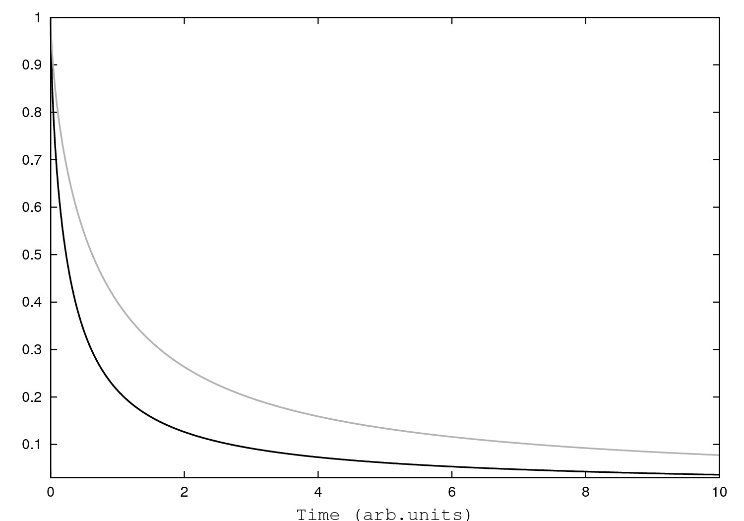
Figure 3: Plot of $p_{n_{0}}^{0.7}(t)$ (in black) and $\mathfrak{p}_{n_{0}}^{0.7}(t)$ (in grey), with $n_{0}=2$.

In order to solve the equation

$$\begin{cases}\frac{d^{\nu}}{dt^{\nu}}\mathfrak{p}_{n_{0}-1}(t)=-2\mu\mathfrak{p}_{n_{0}-1}(t)+\mu E_{\nu,1}(-\mu t^{\nu}),\\ \mathfrak{p}_{n_{0}-1}(0)=0,\end{cases}$$ (3.24)

we resort to the Laplace transform and obtain that

$$\mathcal{L}\left\{\mathfrak{p}_{n_{0}-1}^{\nu}\right\}(z) =\mu z^{\nu-1}\frac{1}{z^{\nu}+\mu}\cdot\frac{1}{z^{\nu}+2\mu}$$ (3.25)

$$=z^{\nu-1}\left(\frac{1}{z^{\nu}+\mu}-\frac{1}{z^{\nu}+2\mu}\right).$$

By inverting (3.25) we extract the following result

$$\mathfrak{p}_{n_{0}-1}^{\nu}(t)=E_{\nu,1}(-\mu t^{\nu})-E_{\nu,1}(-2\mu t^{\nu}).$$ (3.26)

By the same technique we solve

$$\begin{cases}\frac{d^{\nu}}{dt^{\nu}}\mathfrak{p}_{n_{0}-2}(t)=-3\mu\mathfrak{p}_{n_{0}-2}(t)+2\mu\left[E_{\nu,1}(-\mu t^{\nu})-E_{\nu,1}(-2\mu t^{\nu})\right],\\ \mathfrak{p}_{n_{0}-2}(0)=0,\end{cases}$$ (3.27)

thus obtaining

$$\mathcal{L} \left\{\mathfrak{p}_{n_{0}-2}^{\nu}\right\}(z)=2\mu z^{\nu-1}\left[\frac{1}{z^{\nu}+\mu}-\frac{1}{z^{\nu}+2\mu}\right]\frac{1}{z^{\nu}+3\mu}$$ (3.28)

$$=2\mu z^{\nu-1}\left[\left(\frac{1}{z^{\nu}+\mu}-\frac{1}{z^{\nu}+3\mu}\right)\frac{1}{2\mu}-\left(\frac{1}{z^{\nu}+2\mu}-\frac{1}{z^{\nu}+3\mu}\right)\frac{1}{\mu}\right]$$

$$=\frac{z^{\nu-1}}{z^{\nu}+\mu}-2\frac{z^{\nu-1}}{z^{\nu}+2\mu}+\frac{z^{\nu-1}}{z^{\nu}+3\mu}.$$

In light of (3.28), we infer that

$$\mathfrak{p}_{n_{0}-2}^{\nu}(t)=E_{\nu,1}(-\mu t^{\nu})-2E_{\nu,1}(-2\mu t^{\nu})+E_{\nu,1}(-3\mu t^{\nu}).$$ (3.29)

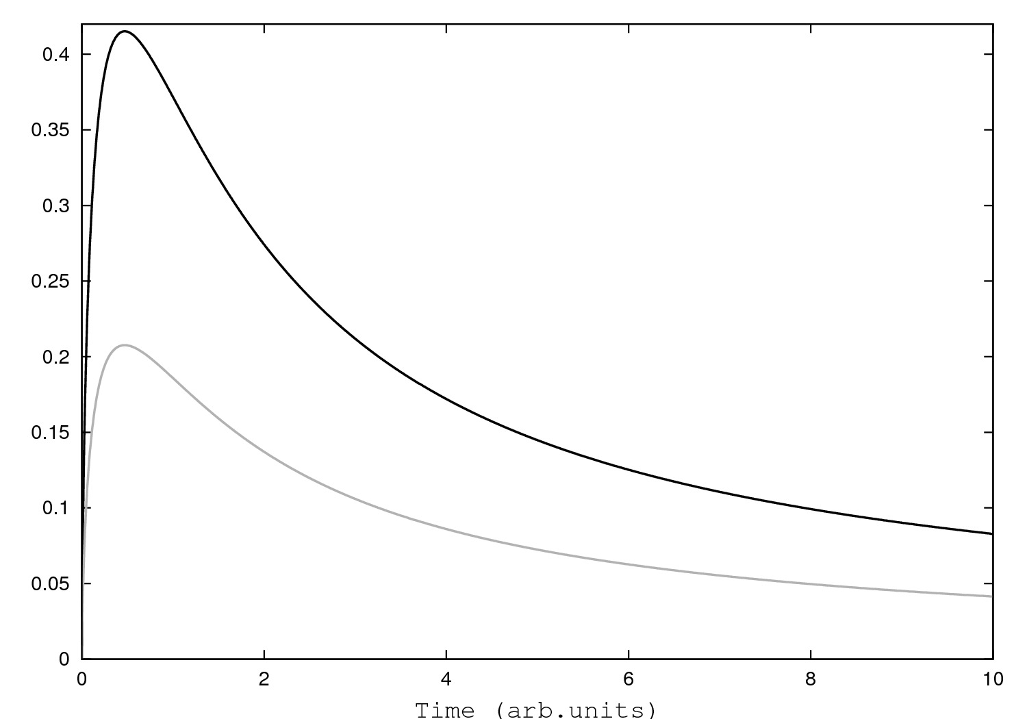
Figure 4: Plot of $p_{n_{0}-1}^{0.7}(t)$ (in black) and $\mathfrak{p}_{n_{0}-1}^{0.7}(t)$ (in grey), with $n_{0}=2$.

For all $1\leq n_{0}-m\leq n_{0}$, by similar calculations, we arrive at the general result

$$\mathfrak{p}_{n_{0}-m}^{\nu}(t)=\sum_{l=0}^{m}\binom{m}{l}(-1)^{l}E_{\nu,1}\left(-\left(l+1\right)\mu t^{\nu}\right),\qquad 1\leq n_{0}-m\leq n_{0}.$$ (3.30)

Introducing the notation $n_{0}-m=k$, we rewrite the state probabilities (3.30) in the following manner

$$\mathfrak{p}_{k}^{\nu}(t)=\sum_{l=0}^{n_{0}-k}\binom{n_{0}-k}{l}(-1)^{l}E_{\nu,1}\left(-\left(l+1\right)\mu t^{\nu}\right),\qquad 1\leq k\leq n_{0}.$$ (3.31)

For the extinction probability we must solve the following Cauchy problem

$$\begin{cases}\frac{d^{\nu}}{dt^{\nu}}\mathfrak{p}_{0}(t)=\mu n_{0}\sum_{l=0}^{n_{0}-1}\binom{n_{0}-1}{l}(-1)^{l}E_{\nu,1}\left(-\left(l+1\right)\mu t^{\nu}\right),\\ \mathfrak{p}_{0}(0)=0.\end{cases}$$ (3.32)

The Laplace transform of (3.32) yields

$$z^{\nu}\mathcal{L}\left\{\mathfrak{p}_{0}^{\nu}\right\}(z)=\mu n_{0}\sum_{l=0}^{n_{0}-1}\binom{n_{0}-1}{l}(-1)^{l}\frac{z^{\nu-1}}{z^{\nu}+\mu(l+1)}.$$ (3.33)

The inverse Laplace transform can be written down as

$$\mathfrak{p}_{0}^{\nu}(t)=\mu n_{0}\sum_{l=0}^{n_{0}-1}\binom{n_{0}-1}{l}(-1)^{l}\frac{1}{\Gamma(\nu)}\int_{0}^{t}E_{\nu,1}\left(-(l+1)\mu s^{\nu}\right)(t-s)^{\nu-1}ds.$$ (3.34)

The integral appearing in (3.34) can be suitably evaluated as follows

$$\int_{0}^{t}E_{\nu,1}\left(-(l+1)\mu s^{\nu}\right)(t-s)^{\nu-1}$$ (3.35)

$$=\sum_{m=0}^{\infty}\frac{(-(l+1)\mu)^{m}}{\Gamma(\nu m+1)}\int_{0}^{t}s^{\nu m}(t-s)^{\nu-1}ds$$

$$=\sum_{m=0}^{\infty}\frac{(-(l+1)\mu)^{m}}{\Gamma(\nu m+1)}\frac{t^{\nu\left(m+1\right)}\Gamma(\nu)\Gamma(\nu m+1)}{\Gamma(\nu m+\nu+1)}$$

$$=\frac{\Gamma(\nu)}{(-\mu(l+1))}\sum_{m=0}^{\infty}\frac{(-(l+1)\mu t^{\nu})^{m+1}}{\Gamma(\nu(m+1)+1)}$$

$$=\frac{\Gamma(\nu)}{(-\mu(l+1))}\left[E_{\nu,1}(-(l+1)\mu t^{\nu})-1\right].$$

By inserting result (3.35) into (3.34), we obtain

$$\mathfrak{p}_{0}^{\nu}(t) =n_{0}\sum_{l=0}^{n_{0}-1}\binom{n_{0}-1}{l}\frac{(-1)^{l+1}}{l+1}\left[E_{\nu,1}(-(l+1)\mu t^{\nu})-1\right]$$ (3.36)

$$=\sum_{l=0}^{n_{0}-1}\binom{n_{0}}{l+1}(-1)^{l+1}\left[E_{\nu,1}(-(l+1)\mu t^{\nu})-1\right]$$

$$=\sum_{l=1}^{n_{0}}\binom{n_{0}}{l}(-1)^{l}E_{\nu,1}(-l\mu t^{\nu})-\sum_{l=1}^{n_{0}}\binom{n_{0}}{l}(-1)^{l}$$

$$=1+\sum_{l=1}^{n_{0}}\binom{n_{0}}{l}(-1)^{l}E_{\nu,1}(-l\mu t^{\nu})$$

$$=\sum_{l=0}^{n_{0}}\binom{n_{0}}{l}(-1)^{l}E_{\nu,1}(-l\mu t^{\nu}).$$

Remark 5.

We check that the probabilities (3.31) and (3.36) sum up to unity. We start by analysing the following sum:

$$\sum_{k=1}^{n_{0}}\mathfrak{p}_{k}^{\nu}(t)=\sum_{k=1}^{n_{0}}\sum_{l=0}^{n_{0}-k}\binom{n_{0}-k}{l}(-1)^{l}E_{\nu,1}(-(l+1)\mu t^{\nu}).$$ (3.37)

In order to evaluate (3.37), we resort to the Laplace transform

$$\sum_{k=1}^{n_{0}}\mathcal{L}\left\{\mathfrak{p}_{k}^{\nu}\right\}(z)=\frac{z^{\nu-1}}{\mu}\sum_{k=1}^{n_{0}}\sum_{l=0}^{n_{0}-k}\binom{n_{0}-k}{l}(-1)^{l}\frac{1}{\frac{z^{\nu}}{\mu}+1+l}.$$ (3.38)

By using formula (6) of kirsch (see also knuth, formula (5.41), page 188), we obtain that

$$\sum_{k=1}^{n_{0}}\mathcal{L}\left\{\mathfrak{p}_{k}^{\nu}\right\}(z) =\frac{z^{\nu-1}}{\mu}\sum_{k=1}^{n_{0}}\frac{\Gamma(n_{0}-k+1)}{\left(\frac{z^{\nu}}{\mu}+1\right)\left(\frac{z^{\nu}}{\mu}+2\right)\dots\left(\frac{z^{\nu}}{\mu}+1+n_{0}-k\right)}$$ (3.39)

$$=\frac{z^{\nu-1}}{\mu}\sum_{k=1}^{n_{0}}\frac{\Gamma\left(\frac{z^{\nu}}{\mu}+1\right)\Gamma\left(n_{0}-k+1\right)}{\Gamma\left(\frac{z^{\nu}}{\mu}+1+n_{0}-k\right)}$$

$$=\frac{z^{\nu-1}}{\mu}\sum_{k=1}^{n_{0}}\int_{0}^{1}x^{\frac{z^{\nu}}{\mu}}(1-x)^{n_{0}-k}dx$$

$$=\frac{z^{\nu-1}}{\mu}\int_{0}^{1}x^{\frac{z^{\nu}}{\mu}-1}\left[1-(1-x)^{n_{0}}\right]dx$$

$$=\frac{1}{z}-\frac{z^{\nu-1}}{\mu}\int_{0}^{1}x^{\frac{z^{\nu}}{\mu}-1}(1-x)^{n_{0}}dx$$

$$\overset{\left(-\ln x=y\right)}{=}\frac{1}{z}-\frac{z^{\nu-1}}{\mu}\int_{0}^{\infty}e^{-y\frac{z^{\nu}}{\mu}}\left(1-e^{-y}\right)^{n_{0}}dy$$

$$\overset{\left(y/\mu=w\right)}{=}\frac{1}{z}z^{\nu-1}\int_{0}^{\infty}e^{-wz^{\nu}}\left(1-e^{-\mu w}\right)^{n_{0}}dw$$

$$=\frac{1}{z}-z^{\nu-1}\sum_{k=0}^{n_{0}}\binom{n_{0}}{k}(-1)^{k}\int_{0}^{\infty}e^{-z^{\nu}w-\mu wk}dw$$

$$=\frac{1}{z}-z^{\nu-1}\sum_{k=0}^{n_{0}}\binom{n_{0}}{k}(-1)^{k}\frac{1}{z^{\nu}+\mu k}.$$

The inverse Laplace transform of (3.39) is therefore

$$\sum_{k=1}^{n_{0}}\mathfrak{p}_{k}^{\nu}(t) =1-\sum_{k=0}^{n_{0}}\binom{n_{0}}{k}(-1)^{k}E_{\nu,1}(-\mu kt^{\nu})$$ (3.40)

$$=-\sum_{k=1}^{n_{0}}\binom{n_{0}}{k}(-1)^{k}E_{\nu,1}(-\mu kt^{\nu}).$$

By putting (3.36) and (3.40) together, we conclude that

$$\sum_{k=0}^{n_{0}}\mathfrak{p}_{k}^{\nu}(t)=1,$$ (3.41)

as it should be.

Remark 6.

We observe that, in the linear and sublinear death processes, the extinction probabilities coincide. This implies that although the state probabilities $p_{k}^{\nu}(t)$ and $\mathfrak{p}_{k}^{\nu}(t)$ differ (see figures 3 and 4) for all $1\leq k\leq n_{0}$, we have that

$$\sum_{k=1}^{n_{0}}p_{k}^{\nu}(t)=\sum_{k=1}^{n_{0}}\mathfrak{p}_{k}^{\nu}(t).$$ (3.42)

This can be checked by performing the following sum

$$\sum_{k=1}^{n_{0}}\mathcal{L}\left\{p_{k}^{\nu}(t)\right\}(z)$$ (3.43)

$$=\sum_{k=1}^{n_{0}}\binom{n_{0}}{k}\sum_{r=0}^{n_{0}-k}\binom{n_{0}-k}{r}(-1)^{r}\frac{z^{\nu-1}}{z^{\nu}+\mu(k+r)}$$

$$=\frac{z^{\nu-1}}{\mu}\sum_{k=1}^{n_{0}}\binom{n_{0}}{k}\sum_{r=0}^{n_{0}-k}\binom{n_{0}-k}{r}(-1)^{r}\frac{1}{\frac{z^{\nu}}{\mu}+k+r}$$

$$=\frac{z^{\nu-1}}{\mu}\sum_{k=1}^{n_{0}}\binom{n_{0}}{k}\frac{\left(n_{0}-k\right)!}{\left(\frac{z^{\nu}}{\mu}+k\right)\left(\frac{z^{\nu}}{\mu}+k+1\right)\dots\left(\frac{z^{\nu}}{\mu}+n_{0}\right)}$$

$$=\frac{z^{\nu-1}}{\mu}\sum_{k=1}^{n_{0}}\binom{n_{0}}{k}\frac{\Gamma\left(n_{0}-k+1\right)\Gamma\left(\frac{z^{\nu}}{\mu}+k\right)}{\Gamma\left(\frac{z^{\nu}}{\mu}+n_{0}+1\right)}$$

$$=\frac{z^{\nu-1}}{\mu}\int_{0}^{1}(1-x)^{\frac{z^{\nu}}{\mu}-1}\sum_{k=1}^{n_{0}}\binom{n_{0}}{k}x^{n_{0}-k}(1-x)^{k}dx$$

$$=\frac{z^{\nu-1}}{\mu}\int_{0}^{1}(1-x)^{\frac{z^{\nu}}{\mu}-1}\left(1-x^{n_{0}}\right)dx$$

$$=\frac{1}{z}-\frac{z^{\nu-1}}{\mu}\int_{0}^{1}x^{n_{0}}(1-x)^{\frac{z^{\nu}}{\mu}-1}dx.$$

This coincides with the fourth-to-last step of (3.39) and therefore we can conclude that

$$\sum_{k=1}^{n_{0}}p_{k}^{\nu}(t)=-\sum_{k=1}^{n_{0}}\binom{n_{0}}{k}(-1)^{k}E_{\nu,1}(-\mu kt^{\nu})=\sum_{k=1}^{n_{0}}\mathfrak{p}_{k}^{\nu}(t).$$ (3.44)

3.2.1 Mean value

Theorem 3.

Consider the fractional sublinear death process $\mathfrak{M}^{\nu}(t)$, $t>0$ defined above. The probability generating function $\mathfrak{G}^{\nu}(u,t)=\sum_{k=0}^{n_{0}}u^{k}\mathfrak{p}_{k}^{\nu}(t)$, $t>0$, $|u|\leq 1$, satisfies the following partial differential equation:

$$\frac{\partial^{\nu}}{\partial t^{\nu}}\mathfrak{G}^{\nu}(u,t)=\mu(n_{0}+1)\left(\frac{1}{u}-1\right)\left[\mathfrak{G}^{\nu}(u,t)-\mathfrak{p}_{0}^{\nu}(t)\right]+\mu(u-1)\frac{\partial}{\partial u}\mathfrak{G}^{\nu}(u,t).$$ (3.45)

subject to the initial condition $\mathfrak{G}^{\nu}(u,0)=u^{n_{0}}$, for $|u|\leq 1$, $t>0$.

Proof.

Starting from (3.22), we obtain that

$$\frac{d^{\nu}}{dt^{\nu}}\sum_{k=0}^{n_{0}}u^{k}\mathfrak{p}_{k}^{\nu}(t)$$ (3.46)

$$=-\mu\sum_{k=1}^{n_{0}}u^{k}(n_{0}+1-k)\mathfrak{p}_{k}^{\nu}(t)+\mu\sum_{k=0}^{n_{0}-1}u^{k}(n_{0}-k)\mathfrak{p}_{k+1}^{\nu}(t),$$

so that

$$\frac{\partial^{\nu}}{\partial t^{\nu}}\mathfrak{G}^{\nu}(u,t)={} -\mu(n_{0}+1)\left[\mathfrak{G}^{\nu}(u,t)-\mathfrak{p}_{0}^{\nu}(t)\right]+\mu u\frac{\partial}{\partial u}\mathfrak{G}^{\nu}(u,t)$$ (3.47)

$$+\frac{\mu(n_{0}+1)}{u}\left[\mathfrak{G}^{\nu}(u,t)-\mathfrak{p}_{0}^{\nu}(t)\right]-\mu\frac{\partial}{\partial u}\mathfrak{G}^{\nu}(u,t)$$

$$={} \mu(n_{0}+1)\left(\frac{1}{u}-1\right)\left[\mathfrak{G}^{\nu}(u,t)-\mathfrak{p}_{0}^{\nu}(t)\right]+\mu(u-1)\frac{\partial}{\partial u}\mathfrak{G}^{\nu}(u,t).$$

∎

Theorem 4.

The mean number of individuals $\mathbb{E}\mathfrak{M}^{\nu}(t)$, $t>0$ in the fractional sublinear death process, reads

$$\mathbb{E}\mathfrak{M}^{\nu}(t)=\sum_{k=1}^{n_{0}}\binom{n_{0}+1}{k+1}(-1)^{k+1}E_{\nu,1}(-\mu kt^{\nu}),\qquad t>0,\>\nu\in(0,1].$$ (3.48)

Proof.

From (3.45) and by considering that $\mathbb{E}\mathfrak{M}^{\nu}(t)=\left.\frac{\partial}{\partial u}\mathfrak{G}^{\nu}(u,t)\right|_{u=1}$, we directly arrive at the following initial value problem:

$$\begin{cases}\frac{d^{\nu}}{dt^{\nu}}\mathbb{E}\mathfrak{M}^{\nu}(t)=-\mu(n_{0}+1)\left[1-\mathfrak{p}_{0}^{\nu}(t)\right]+\mu\mathbb{E}\mathfrak{M}^{\nu}(t),\\ \mathbb{E}\mathfrak{M}^{\nu}(0)=n_{0},\end{cases}$$ (3.49)

which can be solved by resorting to the Laplace transform, as follows:

$$\mathcal{L}\left\{\mathbb{E}\mathfrak{M}^{\nu}(t)\right\}(z) =n_{0}\frac{z^{\nu-1}}{z^{\nu}-\mu}+\mu(n_{0}+1)\sum_{k=1}^{n_{0}}\binom{n_{0}}{k}(-1)^{k}\frac{z^{\nu-1}}{z^{\nu}+\mu k}\cdot\frac{1}{z^{\nu}-\mu}$$ (3.50)

$$=n_{0}\frac{z^{\nu-1}}{z^{\nu}-\mu}+\sum_{k=1}^{n_{0}}\binom{n_{0}+1}{k+1}(-1)^{k}\left[\frac{z^{\nu-1}}{z^{\nu}-\mu}-\frac{z^{\nu-1}}{z^{\nu}+\mu k}\right].$$

In (3.50), formula (3.36) must be considered. By inverting the Laplace transform we obtain that

$$\mathbb{E}\mathfrak{M}^{\nu} (t)$$ (3.51)

$$={} n_{0}E_{\nu,1}(\mu t^{\nu})+\sum_{k=1}^{n_{0}}\binom{n_{0}+1}{k+1}(-1)^{k}\left[E_{\nu,1}(\mu t^{\nu})-E_{\nu,1}(-\mu kt^{\nu})\right]$$

$$={} n_{0}E_{\nu,1}(\mu t^{\nu})+E_{\nu,1}(\mu t^{\nu})\sum_{k=1}^{n_{0}}\binom{n_{0}+1}{k+1}(-1)^{k}$$

$$-\sum_{k=1}^{n_{0}}\binom{n_{0}+1}{k+1}(-1)^{k}E_{\nu,1}(-\mu kt^{\nu})$$

$${}= \sum_{k=1}^{n_{0}}\binom{n_{0}+1}{k+1}(-1)^{k+1}E_{\nu,1}(-\mu kt^{\nu}),$$

as desired. ∎

Remark 7.

The mean value (3.48) can also be directly derived as follows.

$$\mathbb{E}\mathfrak{M}^{\nu}(t) =\sum_{k=0}^{n_{0}}k\mathfrak{p}_{k}^{\nu}(t)$$ (3.52)

$$=\sum_{k=1}^{n_{0}}k\sum_{l=0}^{n_{0}-k}\binom{n_{0}-k}{l}(-1)^{l}E_{\nu,1}(-(l+1)\mu t^{\nu})$$

$$=\sum_{k=1}^{n_{0}}k\sum_{l=1}^{n_{0}+1-k}\binom{n_{0}-k}{l-1}(-1)^{l-1}E_{\nu,1}(-\mu lt^{\nu})$$

$$=\sum_{l=1}^{n_{0}}(-1)^{l-1}E_{\nu,1}(-\mu lt^{\nu})\sum_{k=1}^{n_{0}+1-l}k\binom{n_{0}-k}{l-1}.$$

It is now sufficient to show that

$$\sum_{k=1}^{n_{0}+1-l}k\binom{n_{0}-k}{l-1}=\binom{n_{0}+1}{l+1}.$$ (3.53)

Indeed,

$$\sum_{k=1}^{n_{0}+1-l}k\binom{n_{0}-k}{l-1} =\sum_{k=l-1}^{n_{0}-1}(n_{0}-k)\binom{k}{l-1}$$ (3.54)

$$=\sum_{k=l-1}^{n_{0}-1}(n_{0}+1-k-1)\binom{k}{l-1}$$

$$=(n_{0}+1)\sum_{k=l-1}^{n_{0}-1}\binom{k}{l-1}-l\sum_{k=l-1}^{n_{0}-1}\binom{k+1}{l}$$

$$=(n_{0}+1)\sum_{k=l}^{n_{0}}\binom{k-1}{l-1}-l\sum_{k=l+1}^{n_{0}+1}\binom{k-1}{l}$$

$$=(n_{0}+1)\binom{n_{0}}{l}-l\binom{n_{0}+1}{l+1}$$

$$=\binom{n_{0}+1}{l+1}.$$

The crucial step of (3.54) is justified by the following formula

$$\sum_{k=j}^{n_{0}}\binom{k-1}{j-1}=1+\binom{j}{j-1}+\dots+\binom{n_{0}-1}{j-1}=\binom{n_{0}}{j}.$$ (3.55)

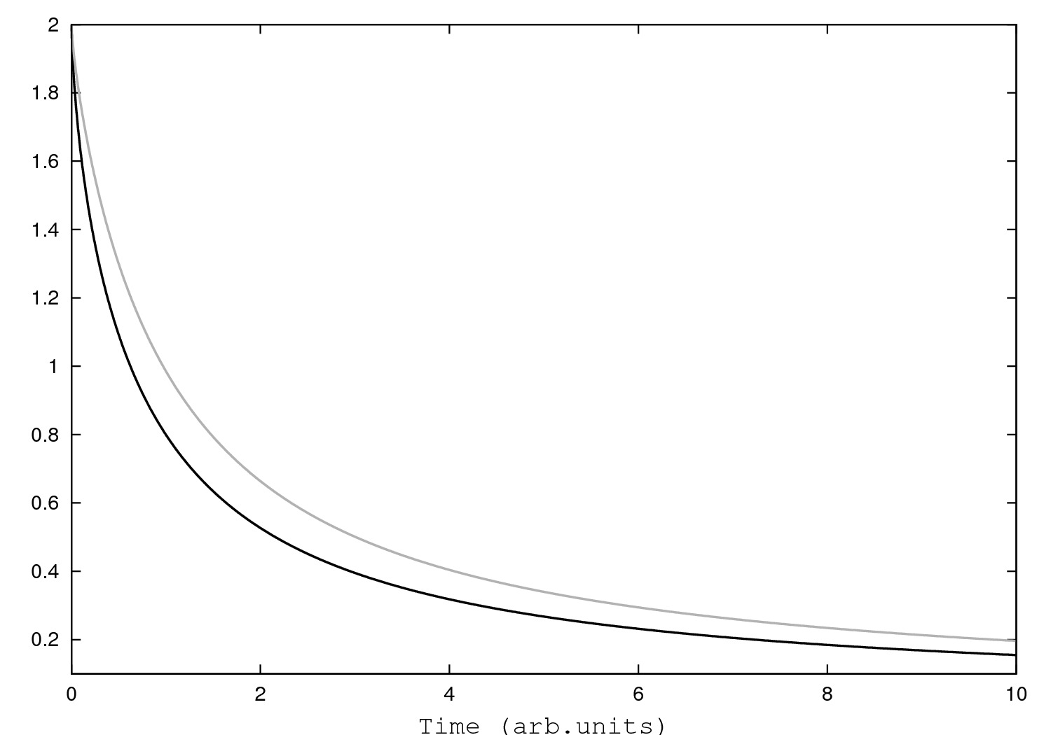
Figure 5: Plot of $\mathbb{E}M^{0.7}(t)$ (in black) and $\mathbb{E}\mathfrak{M}^{0.7}(t)$ (in grey), $n_{0}=2$.

Figure 5 shows that in the sublinear case, the mean number of individuals in the population, decays more slowly than in the linear case, as expected.

Note that (3.48) satisfies the initial condition $\mathbb{E}\mathfrak{M}^{\nu}(0)=n_{0}$. In order to check this, it is sufficient to show that

$$\sum_{k=1}^{n_{0}}\binom{n_{0}+1}{k+1}(-1)^{k+1}=\sum_{r=2}^{n_{0}+1}\binom{n_{0}+1}{r}(-1)^{r}$$ (3.56)

$$=\left[\sum_{r=0}^{n_{0}+1}\binom{n_{0}+1}{r}(-1)^{r}\right]-1+\binom{n_{0}+1}{1}=n_{0}.$$

The details in (3.56) explain also the last step of (3.51).

3.2.2 Comparison of $\mathfrak{M}^{\nu}(t)$ with the fractional linear death process $M^{\nu}(t)$ and the fractional linear birth process $N^{\nu}(t)$

The distributions of the fractional linear and sublinear processes examined above display a behaviour which is illustrated in Table 1 (see also Table 2 for the mean values).

Table 1: State probabilities $p_{k}^{\nu}(t)$ for the fractional linear death process $M^{\nu}(t)$, $t>0$, and $\mathfrak{p}_{k}^{\nu}(t)$ for the fractional sublinear death process $\mathfrak{M}^{\nu}(t)$.

State Probabilities

$p_{n_{0}}^{\nu}(t)=E_{\nu,1}(-\mu n_{0}t^{\nu})$

$\mathfrak{p}_{n_{0}}^{\nu}(t)=E_{\nu,1}(-\mu t^{\nu})$

$p_{n_{0}-1}^{\nu}(t)=n_{0}\left[E_{\nu,1}(-(n_{0}-1)\mu t^{\nu})-E_{\nu,1}(-n_{0}\mu t^{\nu})\right]$

$\mathfrak{p}_{n_{0}-1}^{\nu}(t)=E_{\nu,1}(-\mu t^{\nu})-E_{\nu,1}(-2\mu t^{\nu})$

⋮

$p_{k}^{\nu}(t)=\binom{n_{0}}{k}\sum_{l=0}^{n_{0}-k}\binom{n_{0}-k}{l}(-1)^{l}E_{\nu,1}(-(k+l)\mu t^{\nu})$

$\mathfrak{p}_{k}^{\nu}(t)=\sum_{l=0}^{n_{0}-k}\binom{n_{0}-k}{l}(-1)^{l}E_{\nu,1}\left(-\left(l+1\right)\mu t^{\nu}\right)$

⋮

$p_{1}^{\nu}(t)=n_{0}\sum_{l=0}^{n_{0}-1}\binom{n_{0}-1}{l}(-1)^{l}E_{\nu,1}(-(1+l)\mu t^{\nu})$

$\mathfrak{p}_{1}^{\nu}(t)=\sum_{l=0}^{n_{0}-1}\binom{n_{0}-1}{l}(-1)^{l}E_{\nu,1}\left(-\left(l+1\right)\mu t^{\nu}\right)$

$p_{0}^{\nu}(t)=\sum_{l=0}^{n_{0}}\binom{n_{0}}{l}(-1)^{l}E_{\nu,1}(-l\mu t^{\nu})$

$\mathfrak{p}_{0}^{\nu}(t)=\sum_{l=0}^{n_{0}}\binom{n_{0}}{l}(-1)^{l}E_{\nu,1}(-l\mu t^{\nu})$

The most striking fact about the models dealt with above, is that the linear probabilities decay faster than the corresponding sublinear ones, for small values of $k$; whereas, for large values of $k$, the sublinear probabilities take over and the extinction probabilities in both cases coincide. The reader should also compare the state probabilities of the death models examined here with those of the fractional linear pure birth process (with birth rate $\lambda$ and one progenitor). These read

$$\hat{p}^{\nu}_{k}(t)=\sum_{j=1}^{k}\binom{k-1}{j-1}(-1)^{j-1}E_{\nu,1}(-\lambda jt^{\nu}),\qquad k\geq 1.$$ (3.57)

Note that $\hat{p}_{1}^{\nu}(t)=E_{\nu,1}(-\lambda t^{\nu})$ is of the same form as $\mathfrak{p}_{n_{0}}^{\nu}(t)=E_{\nu,1}(-\mu t^{\nu})$. We now show that

$$\sum_{k=n_{0}+1}^{\infty}\hat{p}_{k}^{\nu}(t) =1-\sum_{k=1}^{n_{0}}\hat{p}_{k}^{\nu}(t)$$ (3.58)

$$=1-\sum_{k=1}^{n_{0}}\sum_{j=1}^{k}\binom{k-1}{j-1}(-1)^{j-1}E_{\nu,1}(-\lambda jt^{\nu})$$

$$=1-\sum_{j=1}^{n_{0}}(-1)^{j-1}E_{\nu,1}(-\lambda jt^{\nu})\sum_{k=j}^{n_{0}}\binom{k-1}{j-1}$$

$$=1-\sum_{j=1}^{n_{0}}(-1)^{j-1}\binom{n_{0}}{j}E_{\nu,1}(-\lambda jt^{\nu})$$

$$=\text{\eqref{extinction} with $\lambda$ replacing $\mu$}.$$

Note that in the above step we used formula (3.55).

Table 2: Mean values for the fractional linear birth $N^{\nu}(t)$, fractional linear death $M^{\nu}(t)$ and fractional sublinear death $\mathfrak{M}^{\nu}(t)$ processes.

$\mathbb{E}N^{\nu}(t)=E_{\nu,1}(\lambda t^{\nu})$

$\mathbb{E}M^{\nu}(t)=n_{0}E_{\nu,1}(-\mu t^{\nu})$

$\mathbb{E}\mathfrak{M}^{\nu}(t)=\sum_{k=1}^{n_{0}}\binom{n_{0}+1}{k+1}(-1)^{k+1}E_{\nu,1}(-\mu kt^{\nu})$

By comparing formulae (3.4) of pol and (3.31) above, we arrive at the conclusion that (for $\lambda=\mu$)

$$\text{Pr}\left\{N^{\nu}(t)=k\mid N^{\nu}(0)=1\right\}$$ (3.59)

$$=\sum_{j=1}^{k}\binom{k-1}{j-1}(-1)^{j-1}E_{\nu,1}(-\lambda_{j}t^{\nu})$$

$$=\text{Pr}\left\{\mathfrak{M}^{\nu}(t)=n_{0}+1-k\mid\mathfrak{M}(0)=n_{0}\right\},\qquad 1\leq k\leq n_{0}.$$

The probability of extinction $\mathfrak{p}_{0}^{\nu}(t)$ corresponds to the probability of the event $\left\{N^{\nu}(t)>n_{0}\right\}$ for the fractional linear birth process.

Acknowledgement: The authors wish to thank Francis Farrelly for having checked and corrected the manuscript. The authors are grateful to the referees for drawing our attention to some relevant references and for useful remarks which improved the presentation of the paper.