The metallicity – redshift relations for emission-line SDSS galaxies: examination of the dependence on the star formation rate

Abstract

We analyse the oxygen abundance and specific star formation rates ($sSFR$) variations with redshift in star-forming SDSS galaxies of different masses. We find that the maximum value of the $sSFR$, $sSFR_{max}$, decreases when the stellar mass, $M_{S}$, of a galaxy increases, and decreases with decreasing of redshift. The $sSFR_{max}$ can exceed the time-averaged $sSFR$ by about an order of magnitude for massive galaxies. The metallicity – redshift relations for subsamples of galaxies with $sSFR$ = $sSFR_{max}$ and with $sSFR$ = 0.1$\times$$sSFR_{max}$ coincide for massive (log($M_{S}$/$M_{\odot}$) $\ga$ 10.5, with stellar mass $M_{S}$ in solar units) galaxies and differ for low-mass galaxies. This suggests that there is no correlation between oxygen abundance and $sSFR$ in massive galaxies and that the oxygen abundance correlates with the $sSFR$ in low-mass galaxies. We find evidence in favour of that the irregular galaxies show, on average, higher $sSFR$ and lower oxygen abundances than the spiral galaxies of similar masses and that the mass – metallicity relation for spiral galaxies differs slightly from that for irregular galaxies. The fact that our sample of low-mass galaxies is the mixture of spiral and irregular galaxies can be responsible for the dependence of the metallicity – redshift relation on the $sSFR$ observed for the low-mass SDSS galaxies. The mass – metallicity and luminosity – metallicity relations obtained for irregular SDSS galaxies agree with corresponding relations for nearby irregular galaxies with direct abundance determinations. We find that the aperture effect does not make a significant contribution to the redshift variation of oxygen abundances in SDSS galaxies.

1 Introduction

It is well established that the oxygen abundance correlates with galaxy mass (or luminosity), O/H = $f$($M_{S}$), in the sense that the higher the galaxy mass (luminosity), the higher the heavy element content (Lequeux et al., 1979; Garnett & Shields, 1987; Skillman et al., 1989; Vila-Costas & Edmunds, 1992; Zaritsky et al., 1994; Pilyugin, 2001b; Guseva et al., 2009; López-Sánchez & Esteban, 2010, among others). In recent years, the number of available spectra of emission-line galaxies has increased dramatically due to the completion of several large spectral surveys, in particular the Sloan Digital Sky Survey (SDSS) (York et al., 2000) . Measurements of emission lines in SDSS spectra have been carried out for abundance determinations and investigation of the luminosity – metallicity relation (e.g. Tremonti et al., 2004). It is discussed whether the mass – metallicity relation can be caused by the galaxy-downsizing effect, where star formation ceases in high-mass galaxies at earlier times and shifts to lower-mass galaxies at later epochs (Cowie et al., 1996). The study of oxygen abundance evolution with redshift in emission-line SDSS galaxies provides strong evidence in favour of the galaxy-downsizing effect (Thuan et al., 2010; Lara-López et al., 2010a; Pilyugin & Thuan, 2011).

It is important to note there are different absolute O/H scales. The empirical metallicity scale is defined by the direct method ($T_{e}$ method) and the empirical calibrations based on it (e.g. Pilyugin, 2001a; Pettini & Pagel, 2004; Pilyugin & Thuan, 2005; Pilyugin et al., 2010). Metallicities derived using calibrations based on photoionisation models (e.g. McGaugh, 1991; Kewley & Dopita, 2002; Kobulnicky & Kewley, 2004) tend to be, systematically higher ($\sim$0.4 dex or even more) than those derived using the direct method (see reviews by López-Sánchez & Esteban, 2010; López-Sánchez et al., 2012). Therefore, there are large discrepancies between oxygen abundances in the SDSS galaxies obtained in different works using different calibrations.

It has been argued that the mass – metallicity relation is due to a more general relation in the 3-dimensional space formed by the stellar mass, gas-phase oxygen abundance and the star formation rate. This 3-dimensional structure is referred to as a Fundamental Plane (FP) by Lara-López et al. (2010b), suggesting that the stellar mass can be expressed as a function of the $SFR$ and O/H, i.e. $M_{S}$ = $f(SFR,$O/H). On the other hand, Mannucci et al. (2010) describes this 3-dimensional space as a surface, the Fundamental Metallicity Relation (FMR) in which the O/H = $f(M_{s},SFR)$. For a further discussion of the 3-dimensional structure of this space see Yates et al. (2012); Lara-López et al. (2013).

It is also known that the mass – metallicity relation changes with redshift $z$. Thus, one can expect that in general the oxygen abundance in a galaxy correlates with three parameters, i.e., O/H = $f$($M_{S}$, $SFR$, $z$). Study of the redshift evolution of oxygen abundances in galaxies of different masses may tell us something about the evolution of galaxies and provide important constrains on the models for the chemical evolution of galaxies. In this paper, we will examine whether the metallicity – redshift relations for SDSS galaxies of different masses are dependent on the star formation rate.

The paper is structured as follows. Selection criteria for the sample of the SDSS galaxies with reliable abundance determinations are reported in Section 2. In Section 3 we establish the redshift evolution of the maximum star formation rates in galaxies of different masses as well the redshift evolutions of oxygen abundances in galaxies of different masses and $sSFR$. The properties of irregular and low-mass spiral galaxies are compared in Section 4. In section 5 we discuss whether the aperture effect makes a significant contribution to the redshift variation of oxygen abundances in the SDSS galaxies. We also estimate the time-averaged values of the $sSFR$ in massive galaxies. The conclusions are given in Section 6.

Throughout the paper, we will be using the following notations for the line fluxes,

$$R_{2}=I_{\rm\rm[OII]\lambda 3727+\lambda 3729}/I_{\rm{\rm H}\beta},$$ (1)

$$N_{2}=I_{\rm\rm[NII]\lambda 6548+\lambda 6584}/I_{\rm{\rm H}\beta},$$ (2)

$$S_{2}=I_{\rm\rm[SII]\lambda 6717+\lambda 6731}/I_{\rm{\rm H}\beta},$$ (3)

$$R_{3}=I_{\rm{\rm[OIII]}\lambda 4959+\lambda 5007}/I_{\rm{\rm H}\beta}.$$ (4)

The stellar masses of galaxies $M_{S}$ are expressed in the solar mass units.

2 Data base

2.1 A sample of SDSS galaxies

Figure 1: Comparison of differences between oxygen (nitrogen) abundances determined in different ways for the sample of reference H ii regions ($E$ sample).

Our study is based on SDSS data. Line flux measurements in SDSS spectra have been carried out by several groups. We use here the data made publicly available by the MPA/JHU group. These data catalogs give line flux measurements, redshifts and various other derived physical properties such as stellar masses for a large sample of SDSS galaxies. The techniques used to construct the catalogues are described in Brinchmann et al. (2004); Tremonti et al. (2004) and various other publications by the same authors.

In a first step, we extract all emission-line objects with measured fluxes in the H$\beta$, H$\alpha$, [O ii]$\lambda\lambda$3727,3729, [O iii]$\lambda$5007, [N ii]$\lambda$6584, [S ii]$\lambda$6717 and [S ii]$\lambda$6731 emission lines. The hydrogen, oxygen, nitrogen and sulfur lines will serve to estimate oxygen and nitrogen abundances relative to hydrogen. The wavelength range of the SDSS spectra is 3800 – 9300 Å so that for nearby galaxies with redshift z $\la$ 0.023, the [O ii]$\lambda$3727+$\lambda$3729 emission line is out of that range. Therefore all SDSS galaxies with z $\la$ 0.023 were excluded. In the other end, distant galaxies with redshift z $\ga$ 0.33, the [S ii]$\lambda$6717+$\lambda$6731 emission line is out of that range. In general, reliable estimates of the oxygen abundance in a SDSS galaxy can be found even if the [O ii]$\lambda$3727+$\lambda$3729 emission line is not available (Pilyugin & Thuan, 2007; Pilyugin & Mattsson, 2011) or if the [S ii]$\lambda$6717+$\lambda$6731 emission line is not measured (Pilyugin et al., 2010). However, our strategy to construct a sample of the SDSS galaxies with rather reliable oxygen abundances requires both these lines. Thus, all galaxies in our total sample have redshifts greater than $\sim$ 0.023 and lower than $\sim$ 0.33. The redshift $z$ and stellar mass M_S of each galaxy were also taken from the MPA/JHU catalogs.

The emission-line fluxes are then corrected for interstellar reddening using the theoretical H$\alpha$/H$\beta$ ratio and the Whitford (1958) interstellar reddening law due to Izotov et al. (1994). We adopt case $B$ recombination with a density of 100 cm^-3, and an electronic temperature of 10⁴ K, which yields a theoretical ratio of H$\alpha$/H$\beta$=2.86 (Osterbrock & Ferland, 2006). In several cases, the derived value of the extinction $C$(H$\beta$) is negative and has then been set to zero.

The [O iii]$\lambda$4959 line is required to obtain the $R_{3}$ value. However, this line is measured with much less accuracy than [O iii]$\lambda$5007 line. Since the [O iii]$\lambda$5007 and $\lambda$4959 lines originate from transitions from the same energy level, their flux ratio is due only to the transition probability ratio, which is very close to 3 (Storey & Zeippen, 2000). Therefore, the value of $R_{3}$ can be estimated as

$$R_{3}=1.33\times\mbox{\rm[O\,{\sc iii}]$\lambda$5007/H$\beta$}$$ (5)

Similarly, the value of $N_{2}$ is estimated without the line [N ii]$\lambda$6548. The [N ii]$\lambda$6584 and $\lambda$6548 lines also originate from transitions from the same energy level and the transition probability ratio for those lines is again close to 3 (Storey & Zeippen, 2000). The value of $N_{2}$ can therefore be estimated as

$$N_{2}=1.33\times\mbox{\rm[N\,{\sc ii}]$\lambda$6584/H$\beta$}$$ (6)

The spectroscopic data so assembled form the basis of the present study.

The intensities of strong, easily measured lines can be used to separate different types of emission-line objects according to their main excitation mechanism. Baldwin et al. (1981) proposed a diagram (the so called BPT classification diagram) where the excitation properties of H ii regions are characterised by plotting the low-excitation [N ii]$\lambda$6584/H$\alpha$ line ratio against the high-excitation [O iii]$\lambda$5007/H$\beta$ line ratio. The exact location of the dividing line between H ii regions and AGNs is still controversial, however (see, e.g., Kewley et al., 2001; Kauffmann et al., 2003; Stasińska et al., 2006). Here we adopt the dividing line suggested by Kauffmann et al. (2003)

$$\log(\mbox{\rm[O\,{\sc iii}]$\lambda$5007/H$\beta$})=\frac{0.61}{\log(\mbox{\rm[N\,{\sc ii}]$\lambda$6584/H$\alpha$})-0.05}+1.3,$$ (7)

which separates objects with H ii spectra from those containing an AGN. By this formula, the suspected AGNs have been excluded from further consideration.

2.2 Abundances

A new method (labelled ”the $C$ method”) for oxygen and nitrogen abundance determination has recently been suggested (Pilyugin et al., 2012c). It is based on the standard assumption that H ii regions with similar strong-line intensities have similar physical properties and abundances. From a sample of reference H ii regions with well-measured ($T_{\rm e}$-based) abundances we choose a counterpart for the considered H ii region by comparison of four combinations of strong-line intensities: $P$ = $R_{3}$/($R_{2}$ + $R_{3}$) (excitation parameter), log$R_{3}$, log($N_{2}$/$R_{2}$), and log($S_{2}$/$R_{2}$) The oxygen and nitrogen abundances, as well as the electron temperature in the studied H ii region may then be assumed to be the same as in its counterpart. To get more reliable abundances, we select a number of reference H ii regions with abundances near those in the counterpart H ii region and then derive the abundance in the studied H ii region through extra-/interpolation.

It has been suggested that reliable oxygen and nitrogen abundances in H ii region can be derived even if the [S ii]$\lambda$6717+$\lambda$6731 emission line is not measured (Pilyugin et al., 2010) or if the [O ii]$\lambda$3727+$\lambda$3729 emission line is not available (Pilyugin & Mattsson, 2011). Hence, the $C$ method can be modified in the following way. To find the counterpart for the H ii region under study, we will compare not the four values that are expressed in terms of the strong line intensities but two sets of three values: 1) log$R_{3}$, $P$ and log($N_{2}$/$R_{2}$) and 2) log$R_{3}$, log$N_{2}$ and log($N_{2}$/$S_{2}$). The oxygen and nitrogen abundances determined with the help of the counterparts selected with the former set of values will be referred to as (O/H)${}_{C_{\rm ON}}$ and (N/H)${}_{C_{\rm ON}}$, while the oxygen and nitrogen abundances determined with the help of the counterparts selected with the latter set of values will be referred to as (O/H)${}_{C_{\rm NS}}$ and (N/H)${}_{C_{\rm NS}}$. Using the collected data with $T_{e}$-based abundances from Pilyugin et al. (2012c) we select a sample of reference H ii regions for which all the absolute differences for oxygen abundances (O/H)${}_{C_{\rm ON}}$ – (O/H)${}_{T_{e}}$ and (O/H)${}_{C_{\rm NS}}$ – (O/H)${}_{T_{e}}$ and for nitrogen abundances (N/H)${}_{C_{\rm ON}}$ – (N/H)${}_{T_{e}}$ and (N/H)${}_{C_{\rm NS}}$ – (N/H)${}_{T_{e}}$ are less 0.1 dex. This sample of reference H ii regions contains 233 objects and will be used for abundance determinations in the following. This sample will be referred to as $E$ sample (etalon sample) below. Hence, here we use the empirical metallicity scale defined by the H ii regions with abundances derived through the direct method ($T_{e}$ method). Comparison between the oxygen abundances (O/H)${}_{C_{NS}}$ and (O/H)${}_{C_{ON}}$ and nitrogen abundances (N/H)${}_{C_{NS}}$ and (N/H)${}_{C_{ON}}$) provides a selection criterion for star-forming galaxies with accurate line fluxes measurements (see below).

The SDSS spectra of distant galaxies are closer to global spectra of galaxies than spectra of single H ii regions. Pilyugin et al. (2012b) have Monte Carlo simulated global spectra of composite nebulae as a mix of spectra of individual components, based on spectra of well-studied H ii regions in nearby galaxies. Abundance analysis of the artificial composite nebulae yielded the conclusion that oxygen and nitrogen abundances determined using the ON and NS calibrations are in good agreement with each other and near (within $\sim$0.2 dex) the mean H$\beta$ luminosity-weighted value of oxygen and nitrogen abundances of individual components of the composite nebula.

2.3 Selection criteria

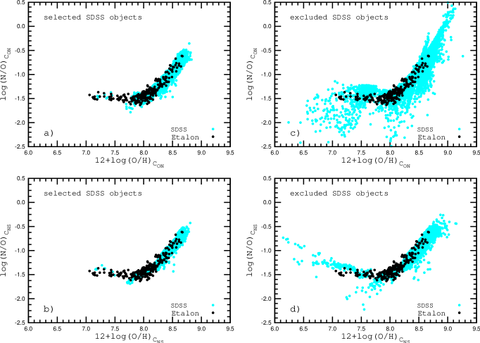
Figure 2: The N/O – O/H diagram. The gray (blue) points in panel $a)$ show the (X/H)${}_{C_{ON}}$ abundances for the selected sample of the SDSS galaxies, the gray (blue) points in panel $b)$ show the (X/H)${}_{C_{NS}}$ abundances. The gray (blue) points in panels $c)$ and $d)$ show the same for the rejected SDSS objects. The dark (black) points in the all panels show the $T_{e}$-based abundances for the sample of reference H ii regions ($E$ sample). (A colour version of this figure is available in the online version.)

Our study is based on SDSS spectra. To study the redshift evolution of oxygen and nitrogen abundances, accurate oxygen and nitrogen abundance determinations are of course a prerequisite. Abundances in H ii regions determined from SDSS spectra suffer from the following problem, however. Line fluxes in SDSS spectra are measured by an automatic procedure, which inevitably introduces large flux errors for some objects. We therefore wish to exclude them from further consideration. A method to recognise such objects relies on the fact that there exist a fundamental H ii region sequence. The emission line properties of photoionised H ii regions are governed by their heavy element content and by the electron temperature distribution within each photoionised nebula. The latter is controlled by the ionising star cluster’s spectral energy distribution and by the chemical composition of the H ii region. The evolution of a giant extragalactic H ii region associated with a star cluster is thus caused by a gradual change over time (due to stellar evolution) of the integrated stellar energy distribution. This phenomenon has been studied in numerous investigations (Stasińska, 1978, 1980; McCall et al., 1985; Dopita & Evans, 1986; Moy et al., 2001; Stasińska & Izotov, 2003; Dopita et al., 2006, among others). The general conclusion from those studies is that H ii regions ionised by star clusters form a well-defined fundamental sequence in different emission-line diagnostic diagrams. The existence of such a fundamental sequence forms the basis for studying various properties of extragalactic H ii regions. First, Baldwin et al. (1981) have suggested the position of an object in some well-chosen emission-line diagrams can be used to separate H ii regions ionised by star clusters from other types of emission-line objects. Second, Pagel et al. (1979) and Alloin et al. (1979) have suggested that the positions of H ii regions in some emission-line diagrams can be calibrated in terms of their oxygen abundances.

Following Thuan et al. (2010) and Mannucci et al. (2010) we adopt here a simple method to recognise star-forming galaxies with accurate line fluxes measurements. It is based on the idea that if i) an object belongs to the fundamental H ii region sequence, and ii) its line fluxes are measured accurately, then the different relations between the line fluxes and the physical characteristic of H ii regions, based on different emission lines, should yield similar physical characteristics (such as electron temperatures and abundances) of that object.

Fig. 1 show comparisons of differences between values of oxygen (nitrogen) abundances determined in various ways for the $E$ sample of reference H ii regions. Fig. 1 also shows that the correlation between differences in oxygen abundances determined in different ways is weak. A correlation between differences in nitrogen abundances determined in different ways is more evident. Although these correlations are not very tight one can expect that the conditions $|$log(O/H)${}_{C_{NS}}$ – log(O/H)${}_{C_{ON}}$$|$ $\leq$ 0.05 and $|$log(N/H)${}_{C_{NS}}$ – log(N/H)${}_{C_{ON}}$$|$ $\leq$ 0.10 allow to select the SDSS objects with more or less reliable abundances. Thus, to select star-forming galaxies with accurate line fluxes measurements, we require that, for each galaxy, the oxygen (O/H)${}_{C_{NS}}$ and (O/H)${}_{C_{ON}}$ and nitrogen (N/H)${}_{C_{NS}}$ and (N/H)${}_{C_{ON}}$ abundances agree.

It should be noted that the $C$ method was developed for H ii regions in the low-density regime. Therefore we include only objects with reliable electron densities $n_{e}$. The electron density is estimated from the sulfur line ratio [S ii]$\lambda$6717/[S ii]$\lambda$6731. According to the five-level atom solution for the S⁺ ion, the [S ii]$\lambda$6717/[S ii]$\lambda$6731 is a reliable indicator of the electron density in the interval from $n_{e}$ $\sim$ 10² cm^-3 to $n_{e}$ $\sim$ 10⁴ cm^-3

$$\log\,n_{e}=8.448-15.101x+14.419x^{2}-5.115x^{3}$$ (8)

where $x$ = [S ii]$\lambda$6717/[S ii]$\lambda$6731. We exclude objects with [S ii]$\lambda$6717/[S ii]$\lambda$6731 $<$ 1.2, i.e., those with $n_{e}$ $\ga$ 170 cm^-3. At densities $n_{e}$ $\la$ 10² cm^-3 the ratio [S ii]$\lambda$6717/[S ii]$\lambda$6731 is almost independent on the electron density and reaches the limit value 1.43. The measured ratio [S ii]$\lambda$6717/[S ii]$\lambda$6731 in some objects is in excess of this limit value, that can be considered as evidence in favour of that the line measurements in the SDSS spectra of this object are not accurate. Therefore the objects with [S ii]$\lambda$6717/[S ii]$\lambda$6731 $>$ 1.55 (expected error in the line measurements is larger $\sim$10%) were also excluded.

Another subset of galaxies were excluded from consideration using the following conditions. In some cases, H ii regions in giant spiral galaxies seem to be catalogued as dwarf galaxies of small dimensions. Thus, if a ”galaxy” has a Petrosian radius less than 3 kpc, this galaxy is then excluded from our list. Further, the aperture correction factor (see below) for some galaxies is $<1$, i.e., the galaxy light within the fiber exceeds the total light of the galaxy. The galaxy light fraction within the fiber is less than 0.7 for the bulk of galaxies. Therefore, the objects with the galaxy light fraction within the fiber higher 0.8 were also excluded from further consideration.

Our final sample contains 98.986 SDSS objects. The O/H – N/O diagram can tell us something about the credibility of our selection criteria and about the reliability of the abundance determinations. Fig. 2 displays the N/O – O/H diagram. The gray (blue points) in the panel $a)$ show the (X/H)${}_{C_{ON}}$ abundances for the selected sample of the SDSS galaxies, the gray (blue points) in the panel $b)$ show the (X/H)${}_{C_{NS}}$ abundances. The dark (black) points (in both panels) show the $T_{e}$-based abundances for the sample of reference H ii regions ($E$ sample). A quick look at Fig. 2 immediately tells us that the selected SDSS galaxies, with very few exceptions, are located within the area outlined by the the reference H ii regions with $T_{e}$-based abundances (as in the case (X/H)${}_{C_{ON}}$ and as in the case (X/H)${}_{C_{NS}}$ abundances in the SDSS galaxies). This suggests that the strategy outlined above allows us to construct a sample of SDSS galaxies with rather reliable oxygen and nitrogen abundances.

Panels $c)$ and $d)$ in Fig. 2 show the N/O – O/H diagrams for the rejected SDSS objects. The positions of rejected objects occupy a much larger area in the (N/O)${}_{C_{ON}}$ – (O/H)${}_{C_{ON}}$ (and (N/O)${}_{C_{NS}}$ – (O/H)${}_{C_{NS}}$) diagram than that outlined by the reference H ii regions, although some rejected objects are located within that area. The weak point of our selection criterion is that we lose some fraction of objects with reliable (O/H)${}_{C_{ON}}$ abundances if only sulfur [S ii]$\lambda$6717 and [S ii]$\lambda$6731 lines measurement involve errors, and some fraction of objects with reliable (O/H)${}_{C_{NS}}$ if only oxygen [O ii]$\lambda\lambda$3727,3729 emission lines measurement involve errors.

The resultant reduced sample is the basis for our study. For clarity and simplicity, only (O/H)${}_{C_{ON}}$ abundances will be considered in the following.

3 The redshift variations of SFR and oxygen abundances in SDSS galaxies

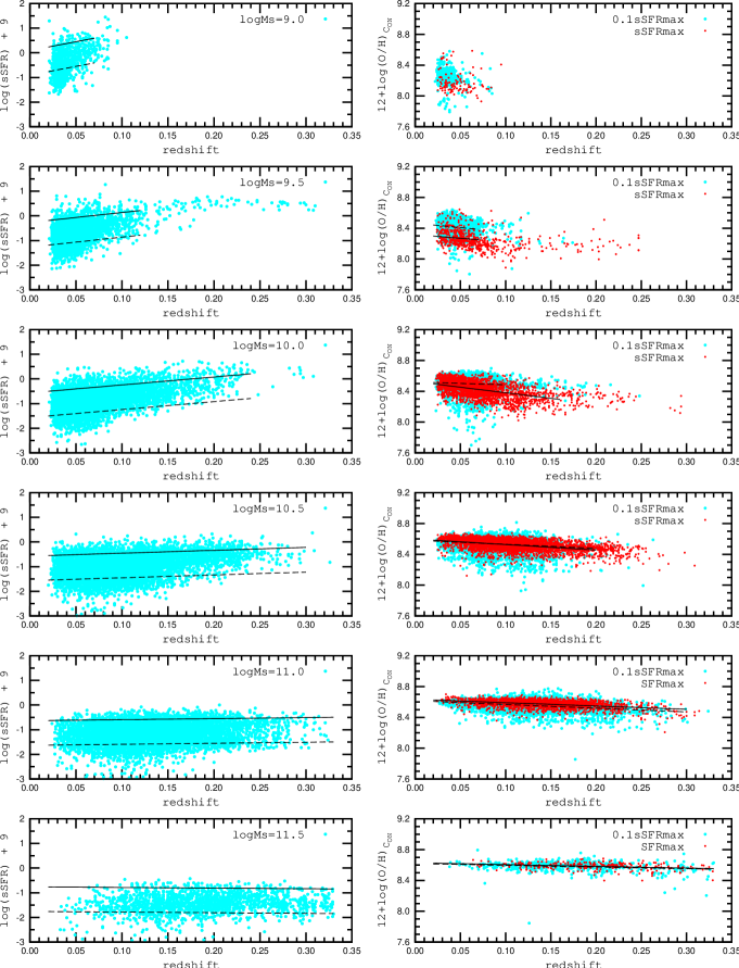
Figure 3: Left panels. Redshift dependence of the $sSFR$ in galaxies of different masses. Light-gray (blue) points are individual galaxies. The solid line is the ”$sSFR$_max – redshift” relation, while the dashed line show the ”0.1$\times$$sSFR$_max – redshift” relation. Right panels. Redshift dependence of the oxygen abundance in galaxies of different masses and different $sSFR$. Dark-gray (red) points are galaxies with log($sSFR$)=log($sSFR_{max}$)$\pm$0.2. The solid line is the best fit to those data. The light-gray (blue) pints are galaxies with log($sSFR$)=log(0.1$\times$$sSFR_{max}$)$\pm$0.2, while the dashed line is the best fit to the data. (A colour version of this figure is available in the online version.)

3.1 Specific star formation rate

The specific star formation rate $sSFR$ is defined as the $SFR$ per unit stellar mass in a galaxy, i.e., $sSFR$ = $SFR$/$M_{S}$. In estimating $SFR$s from the H$\alpha$ luminosity we adopt the calibration suggested by Kennicutt (1998)

$$SFR\;\;({\rm M_{\odot}}{\rm yr^{-1}})=\frac{L_{H{\alpha}}\;\;({\rm W})}{1.27\times 10^{34}},$$ (9)

where

$$L_{H{\alpha}}=4{\pi}d^{2}F_{H{\alpha}}^{cor},$$ (10)

is the H$\alpha$ luminosity. In equation (10) $d$ is the distance to a galaxy, and $F_{H{\alpha}}^{cor}$ is the H$\alpha$ flux corrected for extinction and aperture effect.

The reddening-corrected H$\beta$ flux $F_{\rm{\rm H}\beta}^{O}$ is obtained from the observed $F_{\rm{\rm H}\beta}^{obs}$ flux using the relation (Blagrave et al., 2007)

$$\log(F_{\rm{\rm H}\beta}^{obs}/F_{\rm{\rm H}\beta}^{O})=-C_{\rm\rm H\beta},$$ (11)

where $C$(H$\beta$) is the extinction coefficient. The generic reddening-corrected flux ratio is assumed to be $F_{\rm{\rm H}\alpha}^{O}$/$F_{\rm{\rm H}\beta}^{O}$ = 2.86.

In addition to the extinction correction, the H$\alpha$ luminosity also requires an aperture correction to account for the fact that only a limited amount of emission from a galaxy is detected through the 3” diameter fiber. We estimate the aperture correction factor $A$ using the aperture correction method from Hopkins et al. (2003)

$$A=10^{-0.4(r_{Petro}-r_{fiber})},$$ (12)

where $r_{fiber}$ and $r_{Petro}$ are $r$-band fiber and Petrosian magnitudes. This correction is based on the assumption that the emission line flux can be traced overall by the $r$-band emission. The aperture-corrected H$\alpha$ flux is $F_{\rm{\rm H}\alpha}^{cor}$ = $A$ $\times$ $F_{\rm{\rm H}\alpha}^{O}$.

Distances to galaxies were calculated from

$$d=\frac{cz}{H_{0}},$$ (13)

where $d$ is the distance in Mpc, $c$ the speed of light in km s^-1, and $z$ the redshift. $H_{0}$ is the Hubble constant, here assumed to be equal to 72 ($\pm$8) km s^-1 Mpc^-1 (Freedman et al., 2001).

3.2 The redshift variations of $sSFR$s and oxygen abundances in galaxies of different masses

Studies of the redshift evolution of the $SFR$s in the SDSS galaxies encounter selection-effect problems in the sense that the weak hydrogen emission line luminosity cannot be measured in the distant objects. The lower limit of the measured H$\beta$ luminosity at the redshift $z$=0.25 is three orders of magnitude higher than that at $z$=0.01 (see, for example, Fig.7 in Pilyugin et al. (2012a)). To avoid this selection effect we will consider primarily the redshift evolution of the maximum value of the specific star formation rate $sSFR_{max}$ in galaxies of different masses.

We consider six stellar-mass bins centered on the values log$M_{s}$ = 9.0, 9.5, 10.0, 10.5, 11.0, 11.5 with interval width +/- 0.2 dex. The left panels in Fig. 3 show the redshift variations of $sSFR$s in galaxies of different masses. Light-gray (blue) points are individual galaxies. The solid line is the linear ”$sSFR_{max}$ – redshift” relation. This relation has been obtained as follows. As a first step, the average value of the $sSFR$ has to be found. In a second step, the galaxies with $sSFR$s lower than the average value have to be rejected and a new average $sSFR$ value has to be obtained. In a third step, the galaxies with the $sSFR$s lower than the new average value is rejected and a ”$sSFR$ – redshift” relation is then obtained. The fourth step is to reject the galaxies with the $sSFR$s below this relation and thus a final ”$sSFR_{max}$ – redshift” relation has been obtained. In the deriving the final ”$sSFR_{max}$ – redshift” relation the objects with deviations exceeding the mean value of deviations by a factor three were excluded. Hence, the final ”$sSFR_{max}$ – redshift” is determined using around 5-10% of galaxies in a fixed mass interval. In the first and second steps we use the average $sSFR$ value rather than ”$sSFR$ – redshift” relation in order to exclude the objects with low $sSFR$s in an attempt to overcome the selection effect. The dashed lines in the left panels in Fig. 3 show the ”0.1$\times$$sSFR_{max}$ – redshift” relations.

The left panels in Fig. 3 shows that the maximum specific star formation rate correlates with the stellar mass of a galaxy: the value of the $sSFR_{max}$ decreases with increasing of the $M_{S}$. This nicely confirms the galaxy downsizing effect, where star formation ceases in high-mass galaxies at earlier times and shifts to lower-mass galaxies at later epochs (Cowie et al., 1996).

The right panels in Fig. 3 show the redshift variations of the oxygen abundance in galaxies of different masses and different $sSFR$s. Dark-gray (red) points are galaxies with $sSFR$s close to $sSFR_{max}$, i.e., galaxies which are located within +/-0.2 dex along the solid line in the corresponding left panel in Fig. 3. The solid line is the linear best fit to those data. The light-gray (blue) pints are galaxies with $sSFR$s close to 0.1$\times$$sSFR_{max}$, i.e., galaxies which are located within the band of width +/-0.2 dex along the dashed line in the corresponding left panel in Fig. 3. The dashed line is the best fit to those data.

A closer look at Fig. 3 reveals that the metallicity – redshift relations for massive galaxies (log$M_{s}$ $\ga$ 10.5) do not depend on the $sSFR$. While the $sSFR$ changes by an order of magnitude (from $sSFR_{max}$ to 0.1$\times$$sSFR_{max}$), the metallicity – redshift relations for those galaxies are similar. This, we interpret as evidence that there is no correlation between oxygen abundance and $sSFR$ in massive galaxies. The metallicity – redshift relation for low-mass galaxies (log$M_{s}$ $\la$ 10.5) on the other hand, depends on the $sSFR$: the galaxies with highest $sSFR$ show lowest oxygen abundances.

3.3 Comparison to a previous analysis of SFR-dependence of the O/H – $M_{s}$ relation

The mass – metallicity relation of galaxies as a function of (specific) star formation rate has previously been considered in several different studies (Ellison et al., 2008; Lara-López et al., 2010b; Mannucci et al., 2010; Yates et al., 2012; Andrews & Martini, 2013; Lara-López et al., 2013). It is difficult to directly compare those results with ours for two reasons. First, our method for abundance determination differs from that used in other studies. Second, a single mass – metallicity relation for galaxies from a rather large redshift range were constructed in the papers cited above, i.e., the redshift evolution of galaxies is not taken into account. Therefore, we will limit ourselves to comparison of the general picture of the $SFR$-dependence of the mass – metallicity relation. But first we review the results obtained by previous investigators.

Ellison et al. (2008) considered a mass – metallicity relation for SDSS galaxies, binned in specific star formation rate. Metallicities were obtained using the calibration from Kewley & Dopita (2002). They found that at high stellar masses (log$M_{s}$ $\ga$ 10) the mass – metallicity relation exhibits no dependence on the $sSFR$. At lower stellar masses, there is a tendency for galaxies with higher $sSFR$ to have lower metallicities for a given stellar mass. The offset in metallicity from highest to lowest $sSFR$ bins is $\sim$ 0.10-0.15 dex in the stellar mass range 9 $\la$ log$M_{s}$ $\la$ 10.

Mannucci et al. (2010) studied the relation between stellar mass, metallicity and star formation rate for SDSS galaxies with redshifts 0.07 $\la$ $z$ $\la$ 0.30. The oxygen abundances were derived using calibrations based either on the [N ii]$\lambda$6584/H$\alpha$ or on $R_{23}$ = ([O ii]$\lambda$3727 + [O iii]$\lambda$4959,5007)/H$\beta$ parameter. When both calibrations can be used, galaxy metallicity is defined as the average of these two values. Moreover, they selected only galaxies where the two values of metallicity differ no more than 0.25 dex. They found that galaxies with high stellar masses (log$M_{s}$ $\ga$ 10.9) show no correlation between metallicity and star formation rate, while at low stellar masses more active galaxies also show lower metallicity.

Yates et al. (2012) studied the relation between stellar mass, metallicity and star formation rate for SDSS galaxies with redshifts 0.005 $\la$ $z$ $\la$ 0.25. Two metallicity-data sets were used. The oxygen abundances were derived following Mannucci et al. (2010) in the first case and using the catalogued values in SDSS-DR7 in the second case. They found that the metallicity is dependent on star formation rate for a fixed mass, but that the trend is opposite for galaxies in the low and high stellar-mass ends. Low-mass galaxies with high $SFR$ are more metal poor than quiescent low-mass galaxies. Massive galaxies have lower metallicity if their star formation rates are small. Lara-López et al. (2013) have reached a similar conclusion.

Andrews & Martini (2013) considered SDSS galaxies with redshifts 0.027 $\la$ $z$ $\la$ 0.25. It has been assumed that galaxies at a given stellar mass, or simultaneously a given stellar mass and star formation rate, have the same metallicity. The SDSS galaxies were stacked in bins of (1) stellar mass and (2) both stellar mass and star formation rate. The auroral lines were measured in stacked spectra and the abundances were derived using the direct method. They found that the $SFR$-dependence appeared monotonic with stellar mass.

In summary, the general conclusion in previous studies, is that the mass – metallicity relation is dependent of (specific) star formation rate at low stellar masses (Ellison et al., 2008; Mannucci et al., 2010; Yates et al., 2012; Andrews & Martini, 2013; Lara-López et al., 2013). Our results for low-mass galaxies are in agreement with these results. The conclusions by various authors regarding the $SFR$-dependence of the mass – metallicity relation at high stellar masses are controversial, however. On the one hand, Ellison et al. (2008) and Mannucci et al. (2010) have found that at high stellar masses the mass – metallicity relation shows no dependence on (specific) star formation rate. Our results for massive galaxies are in agreement with the conclusions by Ellison et al. (2008) and Mannucci et al. (2010). On the other hand, Yates et al. (2012); Andrews & Martini (2013); Lara-López et al. (2013) have found that at high stellar masses the mass – metallicity relation depends on (specific) star formation rate. Our results for massive galaxies are in conflict with those results.

4 Low-mass galaxies: spirals vs irregulars

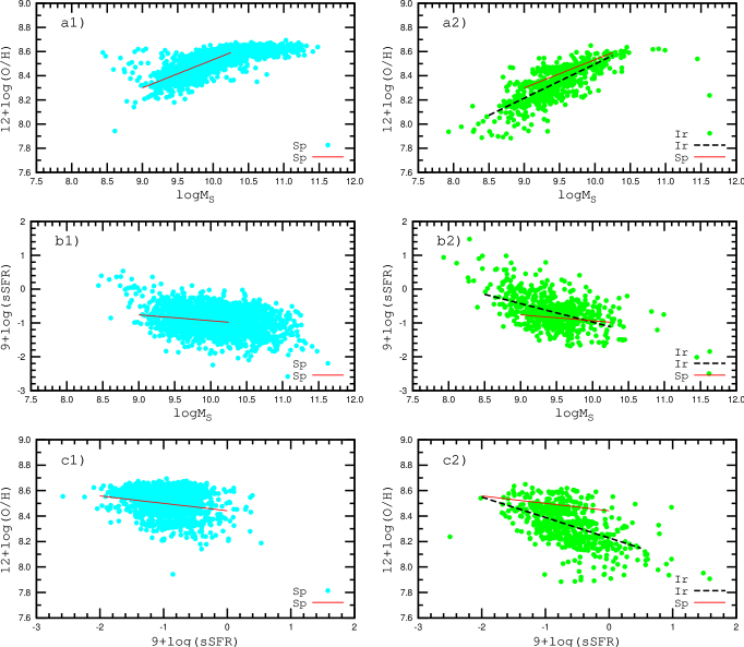
Figure 4: Panel a1). The mass – metallicity diagram for spiral galaxies. Light-gray (blue) points show individual objects, while the dark-gray (red) solid line shows the best fit to galaxies with the masses between log$M_{S}$ = 9.0 and log$M_{S}$ = 10.25. Panel a2). The mass – metallicity relation for irregular galaxies. Light-gray (green) points are individual objects, while the dark (black) dashed line is the best fit to galaxies with masses between log$M_{S}$ = 8.5 and log$M_{S}$ = 10.25. The dark-gray (red) solid line is the same as in panel $a1)$. Panels b1) and b2) show the mass – $sSFR$ diagrams for the same samples of spiral and irregular galaxies, respectively. Panels c1) and c2) show the $sSFR$ – metallicity diagrams for spiral and irregular galaxies, respectively. (A colour version of this figure is available in the online version.)

Thus, there is no correlation between oxygen abundance and $sSFR$ in massive galaxies and the oxygen abundance correlates with the $sSFR$ in low-mass galaxies. The difference in behaviour of massive and low-mass galaxies may be caused by the fact that our sample of low-mass galaxies is a mixture of spiral and irregular galaxies while massive galaxies can be expected to constitute subsamples of galaxies of a single morphological type (spiral galaxies). Below, we compare the properties of irregular and spiral galaxies of low masses.

4.1 Spirals versus irregulars

Let us firstly test whether the spiral and irregular galaxies of similar masses from our sample have different oxygen abundances. Morphological classifications of the SDSS galaxies have been performed within the framework of ”Galaxy Zoo” project. The data catalogue are available in SDSS DR9 database. The project is described in Lintott et al. (2008) and the data release is described in Lintott et al. (2011). The fraction of the votes in each of the six categories (elliptical, clockwise spiral, anticlockwise spiral, edge-on disc, don’t know, merger) is given, along with ”debiased” votes in elliptical and spiral categories and flags identifying systems as classified as spiral, elliptical or uncertain. We assume the votes of spiral galaxies is the sum of the fraction of the votes of clockwise spiral and counterclockwise spiral. Thus, each galaxy is described by five values $f_{X}$ which specify the probability that the galaxy belongs to one of those classes. We assume that the galaxy is a spiral galaxy if the value of $f_{Sp}$ $\ga$ 2/3. Since the class ”irregular galaxies” is not included, we select irregular galaxies by elimination, i.e., we assume that the galaxy is an irregular galaxy if each value $f_{Sp}$, $f_{E}$, $f_{Edge}$, $f_{Merg}$ is less than 1/3.

If there is a difference between oxygen abundances in irregular and spiral galaxies of similar masses then one may expect the mass – metallicity relation for irregular galaxies to be different from that for spiral galaxies. The panel $a1)$ of Fig. 4 shows the mass – metallicity diagram for spiral galaxies at the present epoch (for galaxies with redshifts less than 0.05). Light-gray (blue) points are individual galaxies. Oxygen abundances in massive galaxies do not show significant correlation with galaxy mass. This flattening of the mass – metallicity relation (a plateau at high masses) has previously been observed by Tremonti et al. (2004); Thuan et al. (2010). The luminosity – metallicity relation for nearby spiral galaxies also exhibits a plateau at high luminosities (Pilyugin et al., 2007). Since our goal is to compare the mass – metallicity relations for spiral and irregular galaxies we should derive the relations for a galaxy mass range well populated with both spiral and irregular galaxies, log$M_{S}$ $\la$ 10.25. The best linear least-squares fit to the data for spiral galaxies with masses 10.25 $\ga$ log$M_{S}$ $\ga$ 9.0 is

$$12+\log({\rm O/H})=6.20(\pm 0.05)+0.233(\pm 0.006)\times\log M_{S},$$ (14)

shown in the panel $a1)$ of Fig. 4 as the dark-gray (red) solid line. The small formal errors in the coefficients of Eq.(14) and the rather small mean deviation (0.057 dex) are due to the relatively large number of data points (1494).

The panel $a2)$ of Fig. 4 shows the mass – metallicity diagram for irregular galaxies at the present epoch, $z$ $\la$ 0.05. Light-gray (green) points are individual galaxies. The linear best fit to the data for irregular galaxies with masses 10.25 $\ga$ log$M_{S}$ $\ga$ 8.5

$$12+\log({\rm O/H})=5.68(\pm 0.10)-0.282(\pm 0.011)\times\log M_{S},$$ (15)

is presented in the panel $a2)$ of Fig. 4 by the dark (black) dashed line, while the dark-gray (red) solid line in the lower panel is the same as in the panel $a1)$. Comparison of these slopes, as well as comparison between Eq.(14) and Eq.(15), shows that the mass – metallicity relation for irregular galaxies differs slightly from that for spiral galaxies. Note in passing, however, that the difference is rather small, less than the scatter in abundances in both irregular and spiral galaxies.

Panel $b1)$ of Fig. 4 shows the mass – $sSFR$ diagram for spiral galaxies with redshifts less than 0.05. Light-gray (blue) points are individual galaxies. The best linear least-squares fit to the data for spiral galaxies with masses 10.25 $\ga$ log$M_{S}$ $\ga$ 9.0 is

$$9+\log(sSFR)=0.81(\pm 0.28)-0.17(\pm 0.03)\times\log M_{S},$$ (16)

shown in panel $b1)$ of Fig. 4 as the dark-gray (red) solid line. Panel $b2)$ of Fig. 4 shows the mass – $sSFR$ diagram for irregular galaxies. The linear best fit to the data for irregular galaxies with masses 10.25 $\ga$ log$M_{S}$ $\ga$ 8.5

$$9+\log(sSFR)=4.51(\pm 0.43)-0.55(\pm 0.05)\times\log M_{S},$$ (17)

is presented in panel $b2)$ of Fig. 4 as a dark (black) dashed line, while the dark-gray (red) solid line in the lower panel is the same as in panel $b1)$. Comparison of Eq.(16) and Eq.(17), shows that the mass – $sSFR$ relation for irregular galaxies is steeper than that for spiral galaxies. Spiral and irregular galaxies with masses log$M_{S}$ $\sim$ 10 have similar $sSFR$s, while irregular galaxies with masses log$M_{S}$ $\sim$ 9 have higher $sSFR$s than spiral galaxies of similar masses.

Panel $c1)$ of Fig. 4 shows the $sSFR$ – metallicity diagram for spiral galaxies with redshifts less than 0.05. Light-gray (blue) points are individual galaxies. The best linear least-squares fit to the data for spiral galaxies with masses 10.25 $\ga$ log$M_{S}$ $\ga$ 9.0 is

$$12+\log({\rm O/H})=8.44(\pm 0.01)-0.058(\pm 0.007)\times(\log(sSFR)+9),$$ (18)

shown in panel $c1)$ of Fig. 4 as a dark-gray (red) solid line. Panel $c2)$ of Fig. 4 shows the $sSFR$ – metallicity diagram for irregular galaxies. The linear best fit to the data for irregular galaxies with masses 10.25 $\ga$ log$M_{S}$ $\ga$ 8.5

$$12+\log({\rm O/H})=8.23(\pm 0.01)-0.160(\pm 0.011)\times(\log(sSFR)+9),$$ (19)

is presented in panel $c2)$ of Fig. 4 as a dark (black) dashed line, while the dark-gray (red) solid line in the lower panel is the same as in the panel $c1)$. Comparison of Eq.(18) and Eq.(19), shows that the $sSFR$ – metallicity relation for irregular galaxies is steeper than that for spiral galaxies.

The fact that our sample of low-mass galaxies is a mixture of spiral and irregular galaxies may explain the dependence of the metallicity – redshift relation on the $sSFR$ observed for low-mass SDSS galaxies. The subsample of low-mass galaxies with star formation rates close to $sSFR_{max}$ contains mainly irregular galaxies while the subsample of low-mass galaxies with star formation rates around 0.1$\times$$sSFR_{max}$ contains both irregular and spiral galaxies. Therefore these subsamples show different properties and the metallicity – redshift relations for low-mass galaxies with $sSFR$ = $sSFR_{max}$ and $sSFR$ = 0.1$\times$$sSFR_{max}$ are different.

It is expected that in general the oxygen abundance in a galaxy correlates with three parameters, i.e., O/H = $f$($M_{S}$, $sSFR$, $z$). Using the same data points as in the case of Eq.(14), we have found for spiral galaxies

$$\begin{array}[]{lll}12+\log({\rm O/H})&=&6.18\,(\pm 0.05)+0.240\,(\pm 0.006)\;\log M_{S}\\ &-&0.023\,(\pm 0.005)\;(\log sSFR+9)\\ &-&1.97\,(\pm 0.22)\;z.\\ \end{array}$$ (23)

Again, using the same data points as in the case of Eq.(15), we have found for irregular galaxies

$$\begin{array}[]{lll}12+\log({\rm O/H})&=&5.90(\pm 0.11)+0.262(\pm 0.001)\log M_{S}\\ &-&0.069(\pm 0.009)(\log sSFR+9)\\ &-&2.13(\pm 0.56)z.\\ \end{array}$$ (27)

Comparison of the coefficients in Eq.(23) and Eq.(27) shows that the largest difference (by a factor of $\sim$3) is found for the coefficients in the term with $sSFR$.

4.2 Comparison of the mass – metallicity and luminosity – metallicity relations for SDSS and nearby irregulars

4.2.1 The mass – metallicity relations

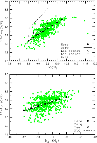
Figure 5: Upper panel. The mass – metallicity relation for irregular galaxies. The gray (green) points show SDSS galaxies (same as in Fig. 4), while dark (black) points show the best fit to data for stellar masses between log$M_{S}$ = 8.5 and log$M_{S}$ = 10.25. The dark (black) solid line is the relation for nearby irregular galaxies from Berg et al. (2012) and the crosses show the mass – metallicity relation for nearby irregulars derived by Lee et al. (2006) with constant mass-to-light ratios, while the plus signs show their relation for $M_{S}$ obtained with colour-dependent mass-to-light ratios. The dark (black) dashed line is the mass – metallicity relation for SDSS galaxies from Zahid et al. (2012). Lower panel. The luminosity – metallicity relation for irregular galaxies. The gray (green) points are the SDSS galaxies, while the dark (black) points show the best fit to data for luminosities between $M_{g}$ = -20 and $M_{g}$ = -17. The dark (black) solid line is the relation for nearby irregular galaxies from Berg et al. (2012) and the crosses show the luminosity – metallicity relation for nearby irregulars according to Lee et al. (2006). The dark (black) dashed line is the $M_{B}$ – (O/H)${}_{T_{e}}$ relation for nearby irregulars from Pilyugin et al. (2004). (A colour version of this figure is available in the online version.)

Fig. 5 shows a comparison between our mass – metallicity and luminosity – metallicity relations for SDSS galaxies and relations obtained for nearby irregular galaxies. The upper panel shows the mass – metallicity diagram, where the gray (green) points are irregular galaxies from the SDSS, the same as in Fig. 4. The dark (black) points show the best fit to the data in the mass range from log$M_{S}$ = 8.5 to log$M_{S}$ = 10.25. Lee et al. (2006) have constructed mass – metallicity and luminosity – metallicity relations for 25 nearby irregular galaxies. The oxygen abundances in 21 of these galaxies were derived through the $T_{e}$ method. They estimated the masses of galaxies from their luminosities in two ways. In the first case they adopted a constant stellar-mass-to-NIR-light ratio and obtained the following mass – metallicity relation,

$$12+\log({\rm O/H})=5.26(\pm 0.27)+0.332(\pm 0.033)\times\log M_{S}.$$ (28)

This relation is shown in the upper panel of Fig. 5 by dark (black) crosses. In the second case they adopted a colour-dependent stellar-mass-to-NIR-light ratio, which yielded the following mass – metallicity relation,

$$12+\log({\rm O/H})=5.65(\pm 0.23)+0.298(\pm 0.030)\times\log M_{S}.$$ (29)

This relation is shown in the upper panel of Fig. 5 by dark (black) plus signs. Furthermore, Berg et al. (2012) measured the temperature sensitive [O iii]$\lambda$4363 line for 31 low luminosity galaxies in the Spitzer Local Volume Legacy survey, and thus determined oxygen abundances using the direct method. They have analysed a ”Combined Select” sample composed of 38 objects (taken from their sample and as well as the literature) with direct oxygen abundances and reliable distance determinations. Stellar masses where estimated from the 4.5 $\mu$m luminosities and $K$ – [4.5] and $B$ – $K$ colours. Using these data, they derived a mass – metallicity relation,

$$12+\log({\rm O/H})=5.61(\pm 0.24)+0.29(\pm 0.03)\times\log M_{S}.$$ (30)

This relation is shown as the dark (black) solid line in the upper panel of Fig. 5.

The upper panel of Fig. 5 shows that our mass – metallicity relation, (O/H)${}_{C_{ON}}$ – $M_{S}$, for SDSS galaxies are consistent with (O/H)${}_{T_{e}}$ – $M_{S}$ relations for nearby irregular galaxies obtained by Lee et al. (2006) and Berg et al. (2012).

Zahid et al. (2012) have estimated oxygen abundances in the SDSS galaxies using the empirical $N2$ calibration after Yin et al. (2007) and have constructed a mass – metallicity relation,

$$12+\log({\rm O/H})=5.585(\pm 0.003)+0.47(\pm 0.01)\times(\log M_{S}-9)$$ (31)

which is shown in the upper panel of Fig. 5 by dark (black) dashed line. This mass – metallicity relation for SDSS galaxies differs significantly from the mass – metallicity relation for SDSS galaxies considered here and from the the mass – metallicity relations for nearby galaxies by Lee et al. (2006) and Berg et al. (2012). This may appear surprising, since Zahid et al. (2012) have estimated oxygen abundances using the purely empirical $N2$ calibration. However, Yin et al. (2007) have noted that the $N2$ index is only a useful metallicity indicator for galaxies with 12 + log(O/H) $\la$ 8.5 as they had no calibrating data points with 12 + log(O/H) $\ga$ 8.5. Hence, the high oxygen abundances (up to 12 + log(O/H) $\sim$ 9.0) obtained by Zahid et al. (2012) with this calibration may be disputed.

4.2.2 The luminosity – metallicity relations

The lower panel of Fig. 5 shows the luminosity – metallicity diagram for irregular galaxies. The gray (green) points show O/H – $M_{g}$ diagram for irregular galaxies from our SDSS sample, where $M_{g}$ is the absolute magnitude of a galaxy in the SDSS photometric band $g$. The dark (black) points show the best fit to those data,

$$12+\log({\rm O/H})=6.41(\pm 0.16)-0.103(\pm 0.009)\times M_{g},$$ (32)

obtained in the luminosity range from $M_{g}$ = -20 to $M_{g}$ = -17. The $B$ – $g$ colour index is $\sim 0.1$ mag only for the star-forming galaxies and the O/H – $M_{g}$ and O/H – $M_{B}$ relations are therefore comparable (Papaderos et al., 2008; Guseva et al., 2009). The O/H – $M_{B}$ relation obtained by Berg et al. (2012) for their ”Combined Select” sample of nearby irregular galaxies,

$$12+\log({\rm O/H})=6.27(\pm 0.21)-0.11(\pm 0.01)\times M_{B},$$ (33)

is shown by the dark (black) solid line. It should be noted that this relation seems to be valid up to $M_{B}$ $\sim$ –8 (Skillman et al., 2013). The relation for nearby irregular galaxies by Lee et al. (2006),

$$12+\log({\rm O/H})=5.94(\pm 0.27)-0.128(\pm 0.017)\times M_{B},$$ (34)

is shown by dark (black) crosses, and that by Pilyugin et al. (2004),

$$12+\log({\rm O/H})=5.80(\pm 0.17)-0.139(\pm 0.011)\times M_{B},$$ (35)

is represented by the dark (black) dashed line.

Our luminosity – metallicity relation, (O/H)${}_{C_{ON}}$ – $M_{g}$, for SDSS galaxies is in satisfactory agreement with (O/H)${}_{T_{e}}$ – $M_{B}$ relations for nearby irregular galaxies obtained in several other studies (Berg et al., 2012; Lee et al., 2006; Pilyugin et al., 2004). It should also be noted that the galaxy metallicity correlates more tightly with its stellar mass than with its luminosity.

5 Discussion

5.1 Does the aperture effect contribute to the redshift dependence of the oxygen abundances?

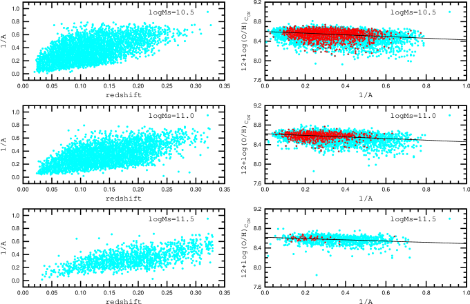
Figure 6: Left panels. Redshift dependence of the galaxy light fraction within the fiber (1/$A$) for galaxies of different masses. Right panels. The oxygen abundance in a galaxy as a function of 1/$A$. Light gray (blue) points are individual objects with redshifts from the full considered range, 0.02 $\la$ $z$ $\la$ 0.33. Dark (black) line is the best fit to those data. Dark gray (red) points are individual objects with redshifts from the range 0.08 – 0.1. (A colour version of this figure is available in the online version.)

The right panels in Fig. 3 show there is a redshift dependence of the oxygen abundance in galaxies of different masses in the sense that the oxygen abundances in distant galaxies are lower than that in nearby galaxies. Chemical evolution of galaxies is usually considered the only reason for the redshift variation of the oxygen abundance in galaxies. In the case of the SDSS galaxies there seems to be another effect that could make a contribution to this redshift dependence. The SDSS galaxy spectra span a relatively wide range of redshifts. There is thus an aperture-redshift effect present in the SDSS data (all spectra are obtained with 3-arcsec-diameter fibers). At a low redshift the projected aperture diameter is smaller than that at high redshift. This means that, at low redshifts, SDSS spectra can be seen as global spectra of the central parts of galaxies (if the fibers are centered on centers of galaxies), i.e., composite nebulae including H ii regions near the center. At large redshifts, however, SDSS spectra are closer to global spectra of whole galaxies, i.e., spectra of composite nebulae including H ii regions near the center as well as in the periphery. Since there is usually a radial abundance gradient in the discs of spiral galaxies (Vila-Costas & Edmunds, 1992; Zaritsky et al., 1994; Pilyugin et al., 2004, among others), the oxygen abundance in the composite nebulae in distant galaxies may be lower than that in nearby galaxies if the fibers are centered on centers of galaxies.

We estimate the aperture-correction factor $A$ (see Eq.12) to account for the fact that only a limited amount of emission from a galaxy is detected through the 3” diameter fiber. The quantity 1/$A$ is the galaxy light fraction within the fiber. The left panels of Fig. 6 show the redshift dependence of the 1/$A$ for galaxies of different masses. The right panels of Fig. 6 show the oxygen abundance in a galaxy as a function of 1/$A$ for subsamples of galaxies of different masses. Light gray (blue) points a show individual objects with redshifts in the full considered range, 0.02 $\la$ $z$ $\la$ 0.33 and the dark (black) line is the best fit to the data. Dark gray (red) points show individual objects with redshifts in the range 0.08 – 0.1. There is obviously a correlation between the oxygen abundance in a galaxy and the galaxy light fraction within the fiber. The correlations for the full considered redshift range and that for a restricted redshift range are similar. The galaxy light fraction within the fiber also correlates with the redshift. Therefore, the diagrams in Fig. 6 cannot tell us whether the correlation between the oxygen abundance in a galaxy and the galaxy light fraction within the fiber is caused by redshift evolution (enrichment in heavy elements) of galaxies or by the aperture effect or a combination of both.

To solve this dilemma we compare the redshift variation of the oxygen abundance in subsample of galaxies for a given value of the aperture correction factor and that for total sample of galaxies of a given mass. Gray (blue) points in the upper panel of Fig. 7 show the redshift dependence of the oxygen abundance with galaxy masses log$M_{S}$ ranging from 10.25 to 10.75, and 1/$A$ in the range 0.45 $>$ 1/$A$ $>$ 0.35. The dark (black) crosses is the linear best fit to those data

$$12+\log({\rm O/H})=a+b\times z.$$ (36)

Values for the coefficients $a$ and $b$ of Eq.(36) are listed in Table 1. The small statistical uncertainties in the coefficients $a$ and $b$ is due to the large numbers of galaxies in the subsamples. The dark (black) line is the linear best fit to all galaxies within the mass range considered, which essentially coincide with the crosses representing the subsample.

Similar diagrams for the other mass intervals are presented in the middle and lower panels of Fig. 7. Again, the relation O/H – $z$ for the subsample and the total sample of galaxies within the given mass ranges coincide. This means that the aperture effect does not make any significant contribution to the redshift dependence of the oxygen abundance in galaxies. The trend in oxygen abundance with redshift must be caused by the chemical evolution of galaxies, i.e. by the increasing level of astration at low redshifts.

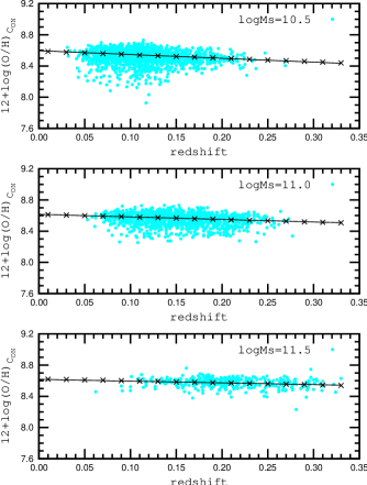
Figure 7: Redshift dependence of the oxygen abundances in galaxies of different masses and an aperture correction factor 0.45 $>$ 1/$A$ $>$ 0.35. Gray (blue) points are individual objects, while the dark (black) crosses show the best fit to the data. The dark (black) line is the best fit to all galaxies in the given mass range. (A colour version of this figure is available in the online version.)

Table 1: Coefficients in the ”oxygen abundance – redshift” relations, 12 + log(O/H) = $a$ + $b$$\times$$z$, for subsamples of galaxies of different stellar masses and different fraction of the light within fiber 1/$A$. (A colour version of this figure is available in the online version.)

mass range	range of 1/$A$	$a$	$b$
log$M_{S}$
10.25 - 10.75	0.45 $>$ 1/$A$ $>$ 0.35	8.591$\pm$0.004	-0.456$\pm$0.037
	1 $>$ 1/$A$ $>$ 0	8.596$\pm$0.001	-0.488$\pm$0.012
10.75 - 11.25	0.45 $>$ 1/$A$ $>$ 0.35	8.615$\pm$0.005	-0.326$\pm$0.034
	1 $>$ 1/$A$ $>$ 0	8.615$\pm$0.002	-0.325$\pm$0.012
11.25 - 11.75	0.45 $>$ 1/$A$ $>$ 0.35	8.623$\pm$0.012	-0.250$\pm$0.057
	1 $>$ 1/$A$ $>$ 0	8.617$\pm$0.004	-0.222$\pm$0.022

The fact that the aperture effect does not play any significant role in the redshift dependence of the oxygen abundance may be explained if the fiber positions are distributed randomly over the images of galaxies. If this is the case, even in nearby galaxies, the fibers may cover both the central and the periphery parts of the galaxies. In such case, the average oxygen abundances in a subsample of SDSS galaxies is more similar to the characteristic oxygen abundance in a galaxy rather than to its central oxygen abundance. It should be noted that many observations with the fibers centered on the galaxy nuclei are excluded from our analysis since the spectra are often classified as AGNs and not star-forming regions.

5.2 Time-averaged specific star formation rate in massive galaxies

The trend in oxygen abundance with redshift is caused by the increasing level of astration (or by the decreasing of the gas-mass fraction $\mu$ = $M_{gas}$/($M_{S}$+$M_{gas}$)) with decreasing of redshift. This provides a possibility to estimate the value of the star formation rate in galaxies of different masses averaged over a fixed time interval. We will consider here only massive galaxies, which can be expected to constitute subsamples of galaxies of a single morphological type (spiral galaxies).

The prediction of the simple (closed-box) model of galactic chemical evolution can be well approximated by a linear expression for $\mu$ values between $\sim$ 0.7 and $\sim$ 0.1. In a real situation, the oxygen abundance is also affected by the mass exchange between a galaxy and its environment (Pagel, 1997). It is commonly accepted that gas infall plays an important role in the chemical evolution of disks of spiral galaxies. Therefore, the application of the simple model to large spiral galaxies may appear unjustified. It is expected that the rate of gas infall onto the disk decreases exponentially with time (Calura et al., 2009, e.g.). It has been shown (Pilyugin & Ferrini, 1998) that the present-day location of a system in the $\mu$ – O/H diagram is governed mainly by its evolution in the recent past, but is weakly dependent of its evolution on long timescales. Therefore, the fact that the present-day location of spiral galaxies is near that predicted by the simple model is not in conflict with infall of gas onto the disk taking place over a long time (the latter is assumed necessary to satisfy the observed abundance distribution function and the age – metallicity relation in the solar neighbourhood) since these observational data reflect the evolution of the system in a distant past. A decrease of $\mu$ by 0.1 results in a increase of oxygen abundance by $\sim$ 0.13 dex (Pilyugin et al., 2006), which lead us to the approximation

$$\Delta(\log({\rm O/H}))\approx-1.3\times\Delta\mu.$$ (37)

The variation in oxygen abundance with redshift is given by the cooefficient $b$ in Eq. (36), the value of $-0.1b$ corresponds to a change in oxygen abundance $\Delta$(log(O/H)) over a redshift interval $\Delta$$z$ = 0.1. At low redshifts, a redshift interval $\Delta$$z$ = 0.1 corresponds to a time interval of about 1 Gyr. Taking Eq.(37) into account, the change of gas-mass fraction $\Delta$$\mu$ over the time interval of 1 Gyr corresponds to 0.077$b$. The gas mass fraction is expressed in terms of the total mass of a galaxy $M_{tot}$. The specific star formation rate is expressed in terms of the stellar mass of a galaxy $M_{S}$. The oxygen abundance 12 + log(O/H) = 8.6 (which is a typical value for massive galaxies, Fig. 7) corresponds to the value of gas mass fraction $\mu$ $\sim$ 0.2 (Pilyugin et al., 2006). This gives $M_{S}$ $\approx$ 0.8$\times$$M_{tot}$. Then the change of gas mass per year expressed in terms of the stellar mass of a galaxy (i.e. the average $sSFR$) is given by the value 10^-10$\times$$b$.

Using the values of $b$ from the Table 1, we estimate the time-averaged $sSFR$s for massive galaxies. We find 9+log($sSFR_{aver}$) $\sim$ -1.31 for galaxies of masses log$M_{S}$ = 10.5 +/-0.2, 9+log($sSFR_{aver}$) $\sim$ -1.49 for galaxies of masses log$M_{S}$ = 11.0 +/-0.2, and 9+log($sSFR_{aver}$) $\sim$ -1.64 for galaxies of masses log$M_{S}$ = 11.5 +/-0.2. Comparison between the $sSFR_{max}$ (Fig. 3) and $sSFR_{aver}$ shows that the $sSFR_{max}$ exceeds the $sSFR_{aver}$ by a factor of 6-7. Since the $sSFR_{max}$ we obtain is not an absolute maximum star formation rate but the mean value for only 5-10% of galaxies with highest $sSFR$s (see Fig. 3), the absolute maximum star formation rate can exceed the time-averaged star formation rate in galaxies of a given mass by about an order of magnitude.

6 Summary and conclusions

In the present study, we have used a sample of 98.986 star-forming SDSS galaxies to examine the dependence of the metallicity – redshift relations on the star formation rate for galaxies of different stellar masses. We determined two values of oxygen and nitrogen abundances for each object using a modified version of the recent counterpart method ($C$ method) (Pilyugin et al., 2012c). The (O/H)${}_{C_{\rm ON}}$ and (N/H)${}_{C_{\rm ON}}$ abundances were derived using the log$R_{3}$, $P$ and log($N_{2}$/$R_{2}$) values to find a counterpart for the studied SDSS galaxy, and, similarly, the (O/H)${}_{C_{\rm NS}}$ and (N/H)${}_{C_{\rm NS}}$ abundances were derived using the log$R_{3}$, log$N_{2}$ and log($N_{2}$/$S_{2}$) values to find a counterpart. In total, we used a sample of 233 reference H ii regions for abundance determinations. The conditions $|$log(O/H)${}_{C_{NS}}$ – log(O/H)${}_{C_{ON}}$$|$ $\leq$ 0.05 and $|$log(N/H)${}_{C_{NS}}$ – log(N/H)${}_{C_{ON}}$$|$ $\leq$ 0.10 were used to select the SDSS objects with the most reliable abundances. Only the (O/H)${}_{C_{\rm ON}}$ abundances were used in our further analyses.

We analysed the redshift dependence of the maximum specific star formation rate $sSFR_{max}$ in SDSS galaxies of different masses. Six stellar mass intervals centered on the values log$M_{s}$ = 9.0, 9.5, 10.0, 10.5, 11.0, 11.5 and width interval widths +/- 0.2 dex were considered. We find that the $sSFR_{max}$ decreases with increasing stellar mass and decreasing redshift. For each mass interval we considered the metallicity – redshift relations for subsamples of galaxies with $sSFR$ $\sim$ $sSFR_{max}$ and with $sSFR$ $\sim$ 0.1$\times$$sSFR_{max}$. These relations coincide for massive (log$M_{S}$ $\ga$ 10.5) galaxies, i.e., the metallicity – redshift relations for massive galaxies are independent of the $sSFR$. On the other hand, these relations differ for low-mass galaxies as the galaxies with $sSFR$ $\sim$ $sSFR_{max}$ have, on average, lower oxygen abundances than galaxies with $sSFR$ $\sim$ 0.1$\times$$sSFR_{max}$.

We also find evidence in favour of irregular galaxies having higher (on average) $sSFR$s and lower oxygen abundances than spiral galaxies of similar masses and that the mass – metallicity relation for spiral galaxies differs slightly from that for irregular galaxies. The mass – metallicity and luminosity – metallicity relations obtained for irregular SDSS galaxies agree with the same for nearby irregular galaxies with direct abundance determinations.

The fact that any sample of low-mass galaxies is likely a mixture of spiral and irregular galaxies can explain the dependence of the metallicity – redshift relation on the $sSFR$.

The redshift variation of the oxygen abundances in galaxies of a given mass allows us to estimate the decrease of gas-mass fractions, i.e. this provides a possibility to estimate the star formation rate in galaxies of different masses averaged over a given time interval. We estimated the time-average specific star formation rates for massive galaxies. We find that the absolute maximum star formation rate can exceed the time-averaged star formation rate in massive galaxies by about an order of magnitude.

Finally, we compared the relations O/H – $z$ for subsample of galaxies within a given range of galaxy light fractions within the spectroscopic fiber and for total sample of galaxies of a given mass. These subsamples show very similar relations, which suggests the aperture effect does not make a significant contribution to the redshift dependence of the oxygen abundances in galaxies. This may be explained by fiber positions being distributed randomly over the images of the galaxies, so in galaxies the fibers may cover both central and periphery parts of different galaxies.In such case, the average oxygen abundances in a subsample of SDSS galaxies is more similar to a characteristic oxygen abundance in a galaxy rather then to its central value.

References

- Alloin et al. (1979) Alloin D., Collin-Souffrin S., Joly M., Vigroux L., 1979, A&A, 78, 200
- Andrews & Martini (2013) Andrews B.H., Martini P., 2013, ApJ, accepted (astro-ph 1211.3418v2)
- Baldwin et al. (1981) Baldwin J.A., Phillips M.M., Terlevich R., 1981, PASP, 93, 5
- Berg et al. (2012) Berg D.A., et al., 2012, ApJ, 754, 98
- Blagrave et al. (2007) Blagrave K.P.M., Martin P.G., Rubin R.H., Dufour R.J., Baldwin J.A., Hester J.J., & Walter D.K. 2007, ApJ, 655, 299
- Brinchmann et al. (2004) Brinchmann J., Charlot S., White S.D.M., Tremonti C., Kauffmann G., Heckman T., Brinkmann J., 2004, MNRAS, 351, 1151
- Calura et al. (2009) Calura F., Pipino A., Chiappini C., Matteucci F., Maiolino R., 2009, A&A, 504, 373
- Cowie et al. (1996) Cowie L.L., Songaila A., Hu E.M., Cohen J.G. 1996, AJ, 112, 839
- Dopita & Evans (1986) Dopita M.A., Evans I.N. 1986, ApJ, 307, 431
- Dopita et al. (2006) Dopita M.A., et al., 2006, ApJS, 167, 177
- Ellison et al. (2008) Ellison S.L., Patton D.R., Simard L., McConnachie A.W., 2008, ApJ, 672. L107
- Freedman et al. (2001) Freedman W.L., Madore B.F., Gibson B.K., et al., 2001, ApJ, 553, 47
- Hopkins et al. (2003) Hopkins A.M., et al., 2003, ApJ, 599, 971
- Garnett & Shields (1987) Garnett D.R., & Shields G.A., 1987, ApJ, 317, 82
- Guseva et al. (2009) Guseva N.G., Papaderos P., Meyer H.T., Izotov Y.I., Fricke K.J., 2009, A&A, 505, 63
- Izotov et al. (1994) Izotov Y.I., Thuan T.X., Lipovetsky V.A., 1994, ApJ, 435, 647
- Kauffmann et al. (2003) Kauffmann G., Heckman T.M., Tremonti C., et al., 2003, MNRAS, 346, 1055
- Kennicutt (1998) Kennicutt R.C., 1998, Annual. Rev. of A&A, 36, 189
- Kewley et al. (2001) Kewley L.J., Dopita M.A., Sutherland R.S., Heisler C.A., Trevena J. 2001 ApJ, 556, 121
- Kewley & Dopita (2002) Kewley L.J., Dopita M.A. 2002, ApJS, 142, 35
- Kobulnicky & Kewley (2004) Kobulnicky H. A., Kewley L. J. 2004, ApJ, 617, 240
- Lara-López et al. (2010a) Lara-López, M. A., et al. 2010a, A&A, 519, L31
- Lara-López et al. (2010b) Lara-López M.A., et al., 2010b, A&A, 521, L53
- Lara-López et al. (2013) Lara-López M.A., López-Sánchez Á.R., Hopkins A.M. 2013, ApJ, 764, 178
- Lee et al. (2006) Lee H., Skillman E.D., Cannon J.M., Jackson D.C., Gehrz R.D., Polomski E.F., Woodward C.E., 2006, ApJ, 647, 970
- Lequeux et al. (1979) Lequeux J., Peimbert M., Rayo J.F., Serrano A., Torres-Peimbert S., 1979, A&A, 80, 155
- Lintott et al. (2008) Lintott C.J., et al., 2008, MNRAS, 389, 1179
- Lintott et al. (2011) Lintott C.J., et al., 2011, MNRAS, 410, 166
- López-Sánchez & Esteban (2010) López-Sánchez Á.R., Esteban C. 2010, A&A, 517, 85
- López-Sánchez et al. (2012) López-Sánchez Á.R., Dopita M.A., Kewley L.J., Zahid H.J., Nicholls D.C., Scharwächter J. 2012, MNRAS, 426, 2630L
- Mannucci et al. (2010) Mannucci F., Cresci G., Maiolino R., Marconi A., Gnerucci A., 2010, MNRAS, 408, 2115
- McCall et al. (1985) McCall M.L., Rybski P.M., Shields G.A. 1985, ApJS, 57, 1
- McGaugh (1991) McGaugh S.S. 1991, ApJ, 380, 140
- Moy et al. (2001) Moy E., Rocca-Volmerange B., Fioc M., 2001, A&A, 365, 347
- Osterbrock & Ferland (2006) Osterbrock D.E., & Ferland G.J. 2006, Astrophysics of gaseous nebulae and active galactic nuclei, 2nd edn., University Science Books, Sausalito, CA
- Pagel (1997) Pagel B.E.J. 1997, Nucleosynthesis and Chemical Evolution of Galaxies (Cambridge: Cambridge Univ. Press)
- Pagel et al. (1979) Pagel B.E.J., Edmunds M.G., Blackwell D.E., Chun M.S., Smith G., 1979, MNRAS, 189, 95
- Papaderos et al. (2008) Papaderos P., Guseva N.G., Izotov Y.I., Fricke K.J., 2008, A&A, 491, 113
- Pettini & Pagel (2004) Pettini M. & Pagel B.E.J. 2004, MNRAS, 348, 59
- Pilyugin & Ferrini (1998) Pilyugin L.S., Ferrini F., 1998, A&A, 336, 103
- Pilyugin (2001a) Pilyugin, L.S. 2001a, A&A, 369, 594
- Pilyugin (2001b) Pilyugin L.S. 2001b, A&A, 374, 412
- Pilyugin et al. (2004) Pilyugin L.S., Vílchez J.M., Contini T. 2004, A&A, 425, 849
- Pilyugin & Thuan (2005) Pilyugin L.S., Thuan T.X. 2005, ApJ, 631, 231
- Pilyugin et al. (2006) Pilyugin L.S., Thuan T.X., Vílchez J.M., 2006, MNRAS, 376, 1139
- Pilyugin & Thuan (2007) Pilyugin L.S., Thuan T.X., 2007, ApJ, 669, 299
- Pilyugin et al. (2007) Pilyugin L.S., Thuan T.X., Vílchez J.M., 2007, MNRAS, 376, 353
- Pilyugin & Thuan (2011) Pilyugin L.S., Thuan T.X., 2011, ApJ, 726, L23
- Pilyugin et al. (2010) Pilyugin L.S., Vílchez J.M., Thuan T.X., ApJ, 2010, 720, 1738
- Pilyugin & Mattsson (2011) Pilyugin L.S., Mattsson L., 2011, MNRAS, 412, 1145
- Pilyugin et al. (2012a) Pilyugin L.S., Zinchenko I.A., Cedrés B., Cepa J., Bongiovanni A., Mattsson L., Vílchez J.M., 2012a, MNRAS, 419, 490
- Pilyugin et al. (2012b) Pilyugin L.S., Vílchez J.M., Mattsson L., Thuan T.X., 2012b, MNRAS, 421, 1624
- Pilyugin et al. (2012c) Pilyugin L.S., Grebel E.K., Mattsson L., 2012c, MNRAS, 424, 2316
- Skillman et al. (1989) Skillman E.D., Kennicutt R.C., Hodge P.W., 1989, ApJ, 347, 875
- Skillman et al. (2013) Skillman E.D., et al., 2013, ApJ, 000, 000 (submitted)
- Stasińska (1978) Stasińska G., 1978, A&A, 66, 257
- Stasińska (1980) Stasińska G., 1980, A&A, 84, 320
- Stasińska & Izotov (2003) Stasińska, G., & Izotov, Y. 2003, A&A, 397, 71
- Stasińska et al. (2006) Stasińska G., Cid Fernandes R., Mateus A., Sodré L., Asari N.V. 2006, MNRAS, 371, 972
- Storey & Zeippen (2000) Storey P.J., Zeippen C.J., 2000, MNRAS, 312, 813
- Thuan et al. (2010) Thuan T.X., Pilyugin L.S., Zinchenko I.A., 2010, ApJ, 712, 1029
- Tremonti et al. (2004) Tremonti C.A., et al., 2004, ApJ, 613, 898
- Vila-Costas & Edmunds (1992) Vila-Costas M.B., Edmunds M.G. 1992, MNRAS, 259, 121
- Whitford (1958) Whitford A.E., 1958, AJ, 63, 201
- Yates et al. (2012) Yates R.M., Kauffmann G., Guo Q., 2012, MNRAS, 422, 215
- Yin et al. (2007) Yin S.Y., Liang Y.C., Hammer F., Brinchmann J., Zhang B., Deng L.C., Flores H., 2007, A&A, 462, 535
- York et al. (2000) York D.G., et al., 2000, AJ, 120, 1579
- Zahid et al. (2012) Zahid H.J., Bresolin F., Kewley L.J., Coil A.L., Davé R., 2012, ApJ, 750, 120
- Zaritsky et al. (1994) Zaritsky D., Kennicutt R.C., Huchra, J.P., 1994, ApJ, 420, 87