CQUeST-2013-0593

TAUP-2963/13

Aging Logarithmic Galilean Field Theories

Seungjoon Hyun¹, Jaehoon Jeong² and Bom Soo Kim³

¹Department of Physics, College of Science, Yonsei University, Seoul 120-749, Korea

²Center for Quantum Spacetime, Sogang University, Seoul 121-742, Korea
³Raymond and Beverly Sackler School of Physics and Astronomy,

Tel Aviv University, 69978, Tel Aviv, Israel

sjhyun@yonsei.ac.kr,   jhjeong@sogang.ac.kr,   bskim@post.tau.ac.il

We analytically compute correlation and response functions of scalar operators for the systems with Galilean and corresponding aging symmetries for general spatial dimensions $d$ and dynamical exponent $z$, along with their logarithmic and logarithmic squared extensions, using the gauge/gravity duality. These non-conformal extensions of the aging geometry are marked by two dimensionful parameters, eigenvalue $\mathcal{M}$ of an internal coordinate and aging parameter $\alpha$.

We further perform systematic investigations on two-time response functions for general $d$ and $z$, and identify the growth exponent as a function of the scaling dimensions $\Delta$ of the dual field theory operators and aging parameter $\alpha$ in our theory. The initial growth exponent is only controlled by $\Delta$, while its late time behavior by $\alpha$ as well as $\Delta$. These behaviors are separated by a time scale order of the waiting time. We attempt to make contact our results with some field theoretical growth models, such as Kim-Kosterlitz model at higher number of spatial dimensions $d$.

1 Introduction

Non-equilibrium growth and aging phenomena are of great interest due to their wide applications across various scientific fields of study, including many body statistical systems, condensed matter systems, biological systems and so on [2]-[5]. They are complex physical systems, and details of microscopic dynamics are widely unknown. Thus it is best to describe these systems with a small number of variables, their underlying symmetries and corresponding universality classes, which have been focus of nonequilibrium critical phenomena.

One particular interesting class is described by the Kardar-Parisi-Zhang (KPZ) equation [6][4]. Recently, this class is realized in a clean experimental setup [7][8], and their exponents for one spatial dimension $d=1$ is confirmed: the roughness $\mathrm{a}=\frac{1}{2}$, the growth $\mathrm{b}=\frac{1}{3}$ and the dynamical $z=\frac{3}{2}$ exponents. Along with the experimental developments, there have been also theoretical developments in the context of aging. The KPZ class reveals also simple aging in the two-time response functions [9][10]. In these works, it is shown that the autoresponse function of the class is well described by the logarithmic (log) and logarithmic squared (log²) extensions of the scaling function with local scale invariance for $d=1$.

In a recent paper [11] based on [12][13], we have considered log extensions of the two-time correlation and response functions of the scalar operators with the conformal Schrödinger and aging symmetries for the spatial dimension $d=2$ and the dynamical exponent $z=2$, in the context of gauge/gravity duality [14][15]. The power-law and log parts are determined by the scaling dimensions of the dual field theory operators, the eigenvalue of the internal coordinate and the aging parameter, which are explained below. Interestingly, our two-time response functions show several qualitatively different behaviors: growth, aging (power-law decaying) or both behaviors for the entire range of our scaling time, depending on the parameters in our theory [11].

We further have made connections to the phenomenological field theory model [9] in detail. The two-time response functions and their log corrections of our holographic model [11] are completely fixed by a few parameters and are valid for $z=2,d=2$, while the field theory model [9] has log² extensions and is valid for $z=\frac{3}{2},d=1$. Closing the gap between these two models from the holographic side is one of the main motivation of this work.

In this paper, we generalize our analysis [11] in two different directions: (1) by applying to general dynamical exponent $z$ (not conformal) as well as to any number of spatial dimensions $d$ and (2) by including log² corrections in two-time response functions. In §2, we first analytically compute the correlation and response functions for general $z$ and $d$ along with their log and log² extensions. Then we add the aging generalizations of our non-conformal results in §3. We try to make contact with KPZ class in §4, and conclude in §5.

2 Logarithmic Galilean Field Theories

Logarithmic conformal field theory(LCFT) is a conformal field theory(CFT) which contains correlation functions with logarithmic divergences. They typically appear when two primary operators with the same conformal dimensions are indecomposable and form a Jordan cell. The natural candidates for the bulk fields, in the holographic dual descriptions of LCFT, of the pair of two primary operators forming Jordan cell are given by a pair of fields with the same spin and a special coupling. After integrating out one of them, it becomes the model with higher derivative terms.

The AdS dual construction of the LCFT was first considered in [18][19][20] using a higher derivative scalar field on AdS background. Recently, higher derivative gravity models on AdS geometry with dual LCFT have got much attention, starting in three dimensional gravity models [21]-[25]. In four and higher dimensional AdS geometry, the gravity models with curvature-squared terms typically contain massless and ghostlike massive spin two fields. When the couplings of the curvature-squared terms are tuned, the massless and massive modes become degenerate and turn into the massless and logarithmic modes [29]. This, so called, critical gravity has the boundary dual LCFT which contains stress-energy tensor operator and its logarithmic counterpart.

More recently, studies on generalizations of LCFT in the context of AdS/CFT correspondence [14][15], in particular the correlation functions of a pair of scalar operators, have been made in two different directions. One is on the non-relativistic LCFT. In [30] the dual LCFT to the scalar field in the Lifshitz background has been investigated. The study on the dual LCFT to the scalar field in the Schrödinger and Aging background was made in [13]. The other is on the LCFT with $\log^{2}$ divergences. Correlation functions with log² corrections have been investigated in several works. In the context of the gravity modes of tricritical point, they are interpreted as rank-3 logarithmic conformal field theories (LCFT) with log² boundary conditions [31]. Explicit action for the rank-3 LCFT is considered in [32]. See also a recent review on these developments in [33].

In this section we would like to accomplish two different things motivated by these developments along with those explained in the introduction. First, we compute correlation and response functions for AdS in light-cone (ALCF) and Schrödinger type gravity theories, which are dual to some non-relativistic field theories with Galilean invariance for general dynamical exponent $z$ and $d$.

Second, we generalize our correlation and response functions with log² as well as log contributions for $z$ and $d$. The log correction has been investigated in [11] in the context of Schrödinger geometry and Aging geometry for $d=2$ and $z=2$ as mentioned in the introduction.

We first consider the ALCF [34][35]. Due to several technical differences, we present our computations in some detail, building up correlation functions §2.1.1, their log extensions §2.1.2 and log² extension §2.1.3. For Schrödinger backgrounds [36][37], we comment crucial differences in §2.2.1. And then we present the correlation functions for $z=2$ in §2.2.2 and for $z=3/2$ in §2.2.3. We summarize our results in §2.3.

2.1 ALCF

Let us turn to the AdS in light-cone (ALCF) with Galilean symmetry studied in [34][35][38]. The case for general $z$ is also considered in [38] for zero temperature and in [39] for finite temperature. The metric is given by

$$ds^{2}=L^{2}\frac{d\vec{x}^{2}-2dtd\xi+du^{2}}{u^{2}}\;,$$ (1)

which is invariant under the space-time translations $P_{i},H$, Galilean boost $K_{i}$,

$$\vec{x}\to\vec{x}-\vec{v}t\;,\qquad\xi\to\xi+\frac{1}{2}(2\vec{v}\cdot\vec{x}-v^{2}t)\;,$$ (2)

scale transformation $D$,

$$t\to\lambda^{z}t\;,\quad\vec{x}\to\lambda\vec{x}\;,\quad u\to\lambda u\;,\quad\xi\to\lambda^{2-z}\xi\;,$$ (3)

and translation along the $\xi$ coordinate, which represents the dual particle number or rest mass. The geometry satisfies vacuum Einstein equations with a negative cosmological constant. The finite temperature generalizations of the ALCF for $z=2$ and $d=2$ have been considered in [40][41][42].

2.1.1 Correlation functions

We compute correlation functions of the geometry (1) by coupling a probe scalar.

$$S=K\int d^{d+2}x\int_{u_{B}}^{\infty}du\sqrt{-g} \left(\partial^{M}\phi^{*}\partial_{M}\phi+m^{2}~{}\phi^{*}\phi\right)\;,$$ (5)

where $K$ is a coupling constant, and $M,N=u,t,\xi,\vec{x}$. We use $u_{B}$ for our boundary cutoff. The field equation of $\phi$ for general $z$ and $d$ is

$$\frac{\partial^{2}\phi}{\partial u^{2}}-(d+1)\frac{1}{u}\frac{\partial\phi}{\partial u}-\left(\frac{m^{2}L^{2}}{u^{2}}+\vec{k}^{2}+2Mw\right)\phi=0\;.$$ (6)

Note that we treat $\xi$ coordinate special and replace all the $\partial_{\xi}$ as $iM$. This is in accord with the fact that the coordinate $\xi$ plays a distinguished role in the geometric realizations of Schrödinger and Galilean symmetries [36][37][38].

The general solution is given by

$$\phi=c_{1}u^{1+d/2}I_{\nu}(qu)+c_{2}u^{1+d/2}K_{\nu}(qu)\;,$$ (7)

where $\nu=\pm\sqrt{(1+d/2)^{2}+L^{2}m^{2}},q^{2}=\vec{k}^{2}+2M\omega$, $I,K$ represent Bessel functions. We choose $K$ over $I$ due to its well defined properties deep in the bulk.

We follow [43][13] to compute correlation functions by introducing a cutoff $u_{B}$ near the boundary and normalizing $f_{\omega,\vec{k}}(u_{B})=1$, which fixes $c=u_{B}^{-1-d/2}K_{\nu}^{-1}(qu_{B})$. We compute an on-shell action to find

$$S[\phi_{0}] =\int d^{d+1}x\frac{L^{d+3}}{u^{d+3}}~{}\phi^{*}(u,t,\vec{x})~{}\frac{u^{2}}{L^{2}}\partial_{u}\phi(u,t,\vec{x})\big{|}_{u_{B}}\;.$$ (8)

Using $k=(\omega,\vec{k})$, $x=(t,\vec{x})$, $ik\cdot x=-i\omega t+i\vec{k}\cdot\vec{x}$ and

$$\phi(u,x)=\int\frac{d\omega}{2\pi}\frac{d^{d}k}{(2\pi)^{d}}~{}e^{ik\cdot x}~{}\phi_{k}(u)~{}\phi_{0}(k)\;,$$ (9)

the onshell action can be rewritten as

$$\int[t,\omega^{\prime},\omega]\int[x,\vec{k}^{\prime},\vec{k}]\quad\phi_{0}^{*}(k^{\prime})\mathcal{F}_{1}(u,k^{\prime},k)\phi_{0}(k)\Big{|}_{u_{B}}\;,$$ (10)

where $\int[t,\omega^{\prime},\omega]\int[x,\vec{k}^{\prime},\vec{k}]=\int dt~{}\frac{d\omega^{\prime}}{2\pi}\frac{d\omega}{2\pi}e^{-i(\omega^{\prime}-\omega)t}\int d^{d}x\int\frac{d^{d}k^{\prime}}{(2\pi)^{d}}\frac{d^{d}k}{(2\pi)^{d}}e^{i(\vec{k}^{\prime}-\vec{k})\cdot\vec{x}}$. $\mathcal{F}_{1}$ is given by

$$\mathcal{F}_{1}(u,k^{\prime},k) =\frac{L^{d+3}}{u^{d+3}}\phi_{k^{\prime}}^{*}(k^{\prime},u)\frac{u^{2}}{L^{2}}\partial_{u}\phi_{k}(k,u)\;.$$ (11)

This function appears again when we construct the log and log² extensions below.

For general $d$ we find

$$\frac{\partial}{\partial u}u^{1+d/2}K_{\nu}(qu)=u^{d/2}\{(1+d/2-\nu)K_{\nu}(qu)-quK_{\nu-1}(qu)\}\;.$$ (12)

One can evaluate the $q$-dependent part of $\mathcal{F}_{1}$ at the boundary, $u=u_{B}$, by expanding it for small $u_{B}$. We obtain the following non-trivial contribution

$$\mathcal{F}_{1}(u_{B},\omega,\vec{k}) =-\frac{2\Gamma(1-\nu)}{\Gamma(\nu)}\left(\frac{L^{d+1}}{u_{B}^{d+2}}\right)\left(\frac{qu_{B}}{2}\right)^{2\nu}+\cdots\;.$$ (13)

Note that the function $\mathcal{F}_{1}$ is only a function of $q(\omega,\vec{k})$ when it is evaluated at the boundary.

By inverse Fourier transform of (13) for an imaginary parameter $M=i\mathcal{M}$, we get the following coordinate space correlation functions for a dual field theory operator $\phi$

$$\langle\phi^{*}(x_{2})\phi(x_{1})\rangle_{\mathcal{F}_{1}} =-2\theta(t_{2})~{}\int\frac{d\omega}{2\pi}\frac{d^{d}k}{(2\pi)^{d}}e^{-i\vec{k}\cdot(\vec{x}_{1}-\vec{x}_{2})}e^{i\omega(t_{1}-t_{2})}\mathcal{F}_{1}(u_{B},k)$$ (14)

$$=\frac{\Gamma(1-\nu)}{\Gamma(\nu)\Gamma(-\nu)}\frac{L^{d+1}\mathcal{M}^{\frac{d}{2}+\nu}}{\pi 2^{\nu-1}u_{B}^{d+2-2\nu}}\cdot\frac{\theta(t_{2})\theta(t_{2}-t_{1})}{(t_{2}-t_{1})^{\frac{d+2}{2}+\nu}}\cdot\exp\left(-{\frac{\mathcal{M}(\vec{x}_{2}-\vec{x}_{1})^{2}}{2(t_{2}-t_{1})}}\right)\;.$$

These are our correlation functions evaluated for general dynamical exponent $z$ and for the number of spatial dimensions $d$, which are direct generalizations of a previous result for $d=2$ and $z=2$ [13]. Note that the result is valid for the field theories with Galilean boost without conformal symmetry. In particular, the parameter $\mathcal{M}$ carries scaling dimensions $[\mathcal{M}]=z-2$, and the exponent is actually dimensionless. This is consistent with the scaling properties written in (4).

The result (14) is independent of $z$, while depending on the number of dimensions $d$. This is expected because the ALCF metric (1) is independent of $z$, which is a special feature for the ALCF. This is not true for Schrödinger background as we see below.

2.1.2 Response functions with log extension

Motivated by the recent interests on LCFT from the holographic point of view [30][11], we consider two scalar fields $\phi$ and $\tilde{\phi}$ in the background (1)

$$S=K\int d^{d+2}x\int_{u_{B}}^{\infty}du\sqrt{-g} \left(\partial^{M}\tilde{\phi}~{}\partial_{M}\phi+m^{2}~{}\tilde{\phi}~{}\phi+\frac{1}{2L^{2}}\tilde{\phi}^{2}\right)\;,$$ (15)

where $u_{B}$ represents a cutoff near the boundary. We take $\partial_{\xi}\phi=-{\cal M}\phi$ and $\partial_{\xi}\tilde{\phi}=-{\mathcal{M}}\tilde{\phi}$.

The field equations for $\phi$ and $\tilde{\phi}$ of the action (15) become

$$2{\cal M}\partial_{t}\phi=-\frac{1}{u^{2}}\mathcal{D}\phi-\vec{\nabla}^{2}\phi+\frac{1}{u^{2}}\tilde{\phi}\;,$$ (16)

$$2{\cal M}\partial_{t}\tilde{\phi}=-\frac{1}{u^{2}}\mathcal{D}\tilde{\phi}-\vec{\nabla}^{2}\tilde{\phi}\;,$$ (17)

where

$$\mathcal{D}=u^{2}\bigg{[}\partial_{u}^{2}-\frac{d+1}{u}\partial_{u}-\frac{m^{2}L^{2}}{u^{2}}\bigg{]}\;,$$ (18)

which is a differential operator for ALCF.

Following [13][30], we construct bulk to boundary Green’s functions $G_{ij}(u,\omega,\vec{k})$

$$\phi(u,x)=\int\frac{d^{d+1}k}{(2\pi)^{d+1}}e^{ik\cdot x}\left[G_{11}(u,k)J(k)+G_{12}(u,k)\tilde{J}(k)\right]\;,$$

$$\tilde{\phi}(u,x)=\int\frac{d^{d+1}k^{\prime}}{(2\pi)^{d+1}}e^{-ik^{\prime}\cdot x}\left[G_{21}(u,k^{\prime})J(k^{\prime})+G_{22}(u,k^{\prime})\tilde{J}(k^{\prime})\right]\;.$$ (19)

We have $G_{21}=0$, which follows from the structure of the equations of motion given in (16) and the action (15). The Green’s functions satisfy

$$\mathrm{D}G_{11} =0\;,\qquad\mathrm{D}G_{12}=G_{22}\;,\qquad\mathrm{D}G_{22}=0\;,$$ (20)

where $\mathrm{D}=\mathcal{D}-q^{2}u^{2}$ and $q=\sqrt{\vec{k}^{2}+2{\cal M}i\omega}$. Solutions of $G_{11}$ and $G_{22}$ are given by

$$G_{11}(u,k_{\mu})=c_{11}~{}u^{1+d/2}K_{\nu}(qu)\;,\qquad G_{22}(u,k_{\mu})=c_{22}~{}u^{1+d/2}K_{\nu}(qu)\;,$$ (21)

where $\nu=\pm\sqrt{(1+d/2)^{2}+m^{2}L^{2}}$. The normalization constants $c_{11}=c_{22}=(u_{B}^{1+d/2}K_{\nu}(qu_{B}))^{-1}$ can be determined by requiring that $G_{11}(u_{B},k_{\mu})=G_{22}(u_{B},k_{\mu})=1$ [43][13].

There exists another Green’s function $G_{12}$ due to a coupling between $\phi$ and $\tilde{\phi}$ in the action (15), which satisfies

$$\mathrm{D}G_{12}=G_{22}\;.$$ (22)

To evaluate $G_{12}$, we use the same methods used in [19][11]. Using

$$\left[\mathrm{D}\;,\frac{d}{d\nu}\right]=2\nu\;,$$ (23)

and the fact that $\mathrm{D}G_{22}=0$, we get

$$\mathrm{D}\left(\frac{1}{2\nu}\frac{d}{d\nu}G_{22}\right)=G_{22}\;.$$ (24)

Thus we have an explicit form.

$$G_{12}=\frac{1}{2\nu}\frac{d}{d\nu}G_{22}=\frac{1}{2\nu}\frac{d}{d\nu}\left(\frac{u^{1+d/2}K_{\nu}(qu)}{u_{B}^{1+d/2}K_{\nu}(qu_{B})}\right)\;.$$ (25)

After plugging the bulk equation of motion into the action (15), the boundary action becomes of the form

$$S_{B} =-K\int d^{d+1}x\frac{L^{d+3}}{u^{d+3}}~{}\tilde{\phi}\frac{u^{2}}{L^{2}}\partial_{u}\phi\Big{|}_{u_{B}}$$

$$=-K\int[t,\omega^{\prime},\omega]\int[x,\vec{k}^{\prime},\vec{k}]~{}~{}\tilde{J}(k^{\prime})\Big{[}\mathcal{F}_{1}(u_{B},k^{\prime},k)J(k)+\mathcal{F}_{2}(u_{B},k^{\prime},k)\tilde{J}(k)\Big{]}\;.$$ (26)

For ALCF, the system has the time translation invariance, thus the time integral is trivially evaluated to give a delta function. The $\mathcal{F}$’s are given by

$$\mathcal{F}_{1} =\frac{L^{d+1}}{u^{d+1}}G_{22}(k^{\prime})~{}\partial_{u}~{}G_{11}(k)\;,$$ (27)

$$\mathcal{F}_{2} =\frac{L^{d+1}}{u^{d+1}}G_{22}(k^{\prime})~{}\partial_{u}~{}G_{12}(k)\;.$$ (28)

We note that $\mathcal{F}_{1}$ leads the same result as (13) and (14).

Let us evaluate $\mathcal{F}_{2}$, which is $\nu$ derivative of $\mathcal{F}_{1}$ given in (25). The result is

$$\langle\phi(x_{2})\phi(x_{1})\rangle_{\mathcal{F}_{2}} =\frac{1}{2\Gamma(\nu+1)}\frac{L^{d+1}\mathcal{M}^{\frac{d}{2}+\nu}}{\pi 2^{\nu-1}u_{B}^{d+2-2\nu}}\cdot\frac{\theta(t_{2})\theta(t_{2}-t_{1})}{(t_{2}-t_{1})^{\frac{d+2}{2}+\nu}}\cdot\exp\left(-{\frac{\mathcal{M}(\vec{x}_{2}-\vec{x}_{1})^{2}}{2(t_{2}-t_{1})}}\right)$$

$$\quad\times\left(1-\nu\frac{\Gamma(\nu)^{\prime}}{\Gamma(\nu)}+\nu\ln[\frac{\mathcal{M}u_{B}^{2}}{2(t_{2}-t_{1})}]\right)\;.$$ (29)

These are our correlation and response functions with log extensions for general $z$ and $d$. This is a direct generalization of the previous result for $d=2$ and $z=2$ [11]. Note that the result is valid for the field theories with Galilean boost without conformal symmetry similar to the result (14). Again it is independent of $z$.

2.1.3 Response functions with log² extensions

Motivated by the recent interests on tricritical log gravity [31], we consider three scalar fields $\phi_{1}$, $\phi_{2}$ and $\phi_{3}$ in the background (1) with the following action

$$S=K\int d^{d+2}x\int_{u_{B}}^{\infty}du\sqrt{-g} \left[\frac{1}{2}\partial^{M}\phi_{2}\partial_{M}\phi_{2}+\partial^{M}\phi_{3}\partial_{M}\phi_{1}+m^{2}\left[\frac{\phi_{2}^{2}}{2}+\phi_{3}\phi_{1}\right]+\frac{\phi_{3}\phi_{2}}{2L^{2}}\right]\;,$$ (30)

where we take $\partial_{\xi}\phi_{i}=-\mathcal{M}\phi_{i}$ for $i=1,2,3$. This action is previously considered in [32] in a different context. The field equations for $\phi$’s of the action (15) become

$$2{\cal M}\partial_{t}\phi_{1}=-\frac{1}{u^{2}}\mathcal{D}\phi_{1}-\vec{\nabla}^{2}\phi_{1}+\frac{1}{u^{2}}\phi_{2}\;,$$ (31)

$$2{\cal M}\partial_{t}\phi_{2}=-\frac{1}{u^{2}}\mathcal{D}\phi_{2}-\vec{\nabla}^{2}\phi_{2}+\frac{1}{u^{2}}\phi_{3}\;,$$ (32)

$$2{\cal M}\partial_{t}\phi_{3}=-\frac{1}{u^{2}}\mathcal{D}\phi_{3}-\vec{\nabla}^{2}\phi_{3}\;,$$ (33)

where $\mathcal{D}$ is given in (18).

We construct the bulk to boundary Green’s function $G_{ij}(u,\omega,\vec{k})$ in terms of $J_{i}(\omega,\vec{k})$ as

$$\phi_{i}(u,x^{\mu})=\int\frac{d^{d}k}{(2\pi)^{d}}\frac{d\omega}{2\pi}e^{ik\cdot x}G_{ij}(u,k)J_{j}(k)\;,$$ (34)

We choose $G_{21}=G_{31}=G_{32}=0$, which is in accord with the structure of the equations of motion given in (31). The Green’s functions satisfy

$$\begin{array}[]{ccc}\mathrm{D}G_{11}=0\;,&\mathrm{D}G_{12}=G_{22}\;,&\mathrm{D}G_{13}=G_{23}\;,\\ \mathrm{D}G_{21}=0\;,&\mathrm{D}G_{22}=0\;,&\mathrm{D}G_{23}=G_{33}\;,\\ \mathrm{D}G_{31}=0\;,&\mathrm{D}G_{32}=0\;,&\mathrm{D}G_{33}=0\;,\end{array}$$ (38)

where $\mathrm{D}=\mathcal{D}-q^{2}u^{2}$ and $q=\sqrt{\vec{k}^{2}+2{\cal M}i\omega}$. The Green’s functions $G_{ii},i=1,2,3$ are

$$G_{ii}(u,k)=c_{ii}~{}u^{1+d/2}K_{\nu}(qu)\;,$$ (39)

where $\nu=\pm\sqrt{(1+d/2)^{2}+m^{2}L^{2}}$ with the same normalization constant given in (8).

There exist other Green’s functions $G_{12},G_{13},G_{23}$ for the action (30), which satisfies

$$\mathrm{D}G_{12}=G_{22}\;,\qquad\mathrm{D}G_{23}=G_{33}\;,\qquad\mathrm{D}G_{13}=G_{23}\;.$$ (40)

In particular, we have

$$\mathrm{D}^{2}G_{13}=G_{33}\;,\quad\mathrm{D}^{3}G_{13}=\mathrm{D}^{2}G_{23}=\mathrm{D}G_{33}=0\;.$$ (41)

To evaluate them, we generalize the methods used in [19][11] to the tricritical case. Using again $\left[\mathrm{D},d/d\nu\right]=2\nu$, and the fact that $\mathrm{D}G_{ii}=0$, we get

$$\mathrm{D}\left(\frac{1}{2\nu}\frac{d}{d\nu}G_{ii}\right)=G_{ii}\;.$$ (42)

Thus

$$G_{12}=\frac{1}{2\nu}\frac{d}{d\nu}G_{22}=\frac{1}{2\nu}\frac{d}{d\nu}\left(\frac{u^{2}K_{\nu}(qu)}{u_{B}^{2}K_{\nu}(qu_{B})}\right)\;,$$ (43)

$$G_{23}=\frac{1}{2\nu}\frac{d}{d\nu}G_{33}=\frac{1}{2\nu}\frac{d}{d\nu}\left(\frac{u^{2}K_{\nu}(qu)}{u_{B}^{2}K_{\nu}(qu_{B})}\right)\;,$$ (44)

$$G_{13}=\frac{1}{4\nu}\frac{d}{d\nu}G_{23}=\frac{1}{4\nu}\frac{d}{d\nu}\left(\frac{1}{2\nu}\frac{d}{d\nu}G_{33}\right)\;.$$ (45)

Note that the last expression has second order derivative of $\nu$, which leads log² contributions.

After plugging the bulk equation of motion into the action (30), the boundary action becomes of the form

$$S_{B} =-K\int d^{d+1}x\frac{L^{5}}{u^{5}}~{}\left(\phi_{2}\frac{u^{2}}{L^{2}}\partial_{u}\phi_{2}+\phi_{3}\frac{u^{2}}{L^{2}}\partial_{u}\phi_{1}\right)\bigg{|}_{u_{B}}$$

$$=-K\int[t,\omega^{\prime},\omega]\int[\vec{x},\vec{k}^{\prime},\vec{k}]~{}~{}J_{i}(k^{\prime}_{\mu})\mathcal{F}_{ij}(u_{B},k^{\prime}_{\mu},k_{\mu})J_{j}(k_{\mu})\;.$$ (46)

The system has time translation invariance, thus the time integral is trivially evaluated to give delta function. The $\mathcal{F}$’s are given by

$$\mathcal{F}_{22} =\frac{L^{3}}{u^{3}}G_{22}(k^{\prime}_{\mu})~{}\partial_{u}~{}G_{22}(k_{\mu})=\mathcal{F}_{1}\;,$$ (47)

$$\mathcal{F}_{23} =\frac{L^{3}}{u^{3}}G_{22}(k^{\prime}_{\mu})~{}\partial_{u}~{}G_{23}(k_{\mu})=\mathcal{F}_{2}\;,$$ (48)

$$\mathcal{F}_{31} =\frac{L^{3}}{u^{3}}G_{33}(k^{\prime}_{\mu})~{}\partial_{u}~{}G_{11}(k_{\mu})=\mathcal{F}_{1}\;,$$ (49)

$$\mathcal{F}_{32} =\frac{L^{3}}{u^{3}}\left(G_{23}(k^{\prime}_{\mu})~{}\partial_{u}~{}G_{22}(k_{\mu})+G_{33}(k^{\prime}_{\mu})~{}\partial_{u}~{}G_{12}(k_{\mu})\right)=\mathcal{F}_{2}\;,$$ (50)

$$\mathcal{F}_{33} =\frac{L^{3}}{u^{3}}\left(G_{23}(k^{\prime}_{\mu})~{}\partial_{u}~{}G_{23}(k_{\mu})+G_{33}(k^{\prime}_{\mu})~{}\partial_{u}~{}G_{13}(k_{\mu})\right)=\mathcal{F}_{3}\;.$$ (51)

Note that the first terms in $\mathcal{F}_{32}$ and $\mathcal{F}_{33}$ are $0$ when evaluated at $u=u_{B}$. We also notice that $\mathcal{F}_{1}$ and $\mathcal{F}_{2}$ are identical to (13) and (28), and thus the corresponding correlation functions (14) and (2.1.2), respectively.

Now we are ready to evaluate $\mathcal{F}_{3}$. Using (45) and (14), we get

$$\langle\phi_{3}(x_{2})\phi_{3}(x_{1})\rangle_{\mathcal{F}_{3}} =\frac{1}{8\nu^{3}\Gamma(\nu)}\frac{L^{d+1}\mathcal{M}^{\frac{d}{2}+\nu}}{\pi 2^{\nu-1}u_{B}^{d+2-2\nu}}\cdot\frac{\theta(t_{2})\theta(t_{2}-t_{1})}{(t_{2}-t_{1})^{\frac{d+2}{2}+\nu}}\cdot\exp\left(-{\frac{\mathcal{M}(\vec{x}_{2}-\vec{x}_{1})^{2}}{2(t_{2}-t_{1})}}\right)$$ (52)

$$\times\left[1+\nu\psi-\nu^{2}(\psi^{2}-\psi^{\prime})+(2\nu^{2}\psi-\nu)\ln[\frac{\mathcal{M}u_{B}^{2}}{2(t_{2}-t_{1})}]-\nu^{2}\ln[\frac{\mathcal{M}u_{B}^{2}}{2(t_{2}-t_{1})}]^{2}\right]\;,$$

where $\psi(\nu)=\frac{\Gamma(\nu)^{\prime}}{\Gamma(\nu)}$. This is our main result in this section, response functions with log and log² extensions, which is valid for general $z$ and $d$. Note also that this result is valid for the systems without non-relativistic conformal invariance. We notice that various coefficients in the square bracket are completely determined once $\nu$ is fixed.

2.2 Schrödinger backgrounds

We first establish the Schrödinger type solutions with Galilean symmetry with $z\neq 2$ following [37], see also [38][36]. Finite temperature generalizations for general $z$ is considered in [39], while those for $z=2$ are considered in [44][45][46][47][48].

The metric at zero temperature is given by

$$ds^{2}=L^{2}\left(-\gamma\frac{dt^{2}}{u^{2z}}+\frac{d\vec{x}^{2}-2dtd\xi+du^{2}}{u^{2}}\right)\;,$$ (53)

which is invariant under the space-time translations $P_{i},H$, Galilean boost $K_{i}$, scale transformation $D$ and translation along the $\xi$ coordinate. Their explicit forms are given in (2) and (3). There exists additional special conformal transformation for $z=2$, which has been focus of previous investigations.

There have been more general class of gravity backgrounds with so-called hyperscaling violation. These backgrounds are described by $ds^{2}=u^{2-2\frac{\theta}{d+1}}\left[-\gamma\frac{dt^{2}}{u^{2z}}+\frac{d\vec{x}^{2}-2dtd\xi+du^{2}}{u^{2}}\right]$ considered in [38], where $\theta$ is a hyperscaling violation exponent. $\theta$ is first introduced in [49] based on [50]. This hyperscaling violation might be also interesting in the general context of aging and growth phenomena. The associated matter fields are a gauge field, a scalar and the non-trivial coupling between them.

The geometry (53) is not a solution of vacuum Einstein equations. Thus we require to support it with some matter fields. One particular example is the ground state of an Abelian Higgs model in its broken phase [37]

$$S=\int d^{d+3}x\sqrt{-g}\left(-\frac{1}{4}F^{2}-\frac{1}{2}|D\Phi|^{2}-V(|\Phi|)\right)\;,$$ (54)

$$V(|\Phi|)=\left(|\Phi|^{2}-v^{2}\right)^{2}-\frac{(d+1)(d+2)}{L^{2}}\;,$$ (55)

$$A_{t}(u)=\frac{\rho_{0}}{u^{z}}\;,\quad\rho_{0}^{2}=\frac{2L^{2}(z-1)(2z+d)\gamma}{z^{2}+e^{2}v^{2}L^{2}}\;,$$ (56)

where $F=dA$, $F^{2}=F^{MN}F_{MN}$, and $d$ is the number of spatial dimensions.

It is not hard to find a different matter system that supports the metric [36].

$$S=\int d^{d+3}x\sqrt{-g}\left(-\frac{1}{4}F^{2}-\frac{m^{2}}{2}A^{2}+\frac{(d+1)(d+2)}{L^{2}}\right)\;,$$ (57)

$$A_{t}(u)=\frac{\rho_{0}}{u^{z}}\;,\quad\rho_{0}^{2}=\frac{2\left(d+2z\right)(z-1)L^{2}\gamma}{3z}\;,\quad m^{2}=\frac{z(3-z)}{L^{2}}\;,$$ (58)

where $A^{2}=A^{M}A_{M}$.

2.2.1 Correlation and response functions with log $\&$ log² extensions

We are interested in constructing correlation and response functions using three different actions, (5), (15) and (30), as in the previous section §2.1. Here we briefly show that the procedure is the same as before. Thus we can compute the logarithmic (squared) extensions by taking a simple $\nu$ derivatives of the correlation function obtained from the action (5).

We start by considering correlation functions of the geometry (53) by coupling a probe scalar with the same action as (5). The field equation for $\phi$ becomes

$$\frac{\partial^{2}\phi}{\partial u^{2}}-(d+1)\frac{1}{u}\frac{\partial\phi}{\partial u}-\left(\frac{m^{2}L^{2}}{u^{2}}+\vec{k}^{2}+2Mw+\gamma M^{2}u^{2-2z}\right)\phi=0\;.$$ (59)

Note $\gamma\neq 0$, which is one of the main differences between the Schrödinger background (53) and ALCF (1). Again, we treat $\xi$ coordinate special and replace all the $\partial_{\xi}$ as $iM$. With this differential equation, one can compute the correlation function $\mathcal{F}_{1}$. For general $z$, analytic solutions are not available. The resulting correlation function for $z=2$ is already computed in [12][13][11], while that of $z=3/2$ is computed below in §2.2.3. Previously, several special cases also have been computed in [38].

To compute the corresponding log and log² extensions, we consider a Schrödinger differential operator

$$\mathrm{D}_{Schr}=u^{2}\bigg{[}\partial_{u}^{2}-\frac{d+1}{u}\partial_{u}-\frac{\nu^{2}-(1+d/2)^{2}}{u^{2}}-q^{2}-\gamma M^{2}u^{2-2z}\bigg{]}\;,$$ (60)

where $q^{2}=\vec{k}^{2}+2M\omega$ and $\nu=\pm\sqrt{(1+d/2)^{2}+L^{2}m^{2}}$ for $z\neq 2$. For the special case $z=2$, we have $\nu=\pm\sqrt{(1+d/2)^{2}+L^{2}m^{2}+\gamma M^{2}}$ from (60). With the differential operator $\mathrm{D}_{Schr}$, we can still use the relation

$$\left[\mathrm{D}_{Schr}\;,\frac{d}{d\nu}\right]=2\nu\;,$$ (61)

to compute the correlation (response) functions with the logarithmic extensions. For that purpose, we use the equations (2.1.2) - (27) with appropriate $G_{11}$ and $G_{22}$. We also get the response functions with the log² extension using (34) - (51) with appropriate $G_{11},G_{22}$ and $G_{33}$.

The upshot is that the logarithmic extensions can be computed by taking one or two derivatives of the correlation functions available. Let us compute these correlation and response functions for $z=2$ and $z=3/2$ in turn.

2.2.2 Conformal Schrödinger backgrounds with $z=2$

We comment for the conformal case $z=2$ here. The differential equation (59) simplifies to

$$\frac{\partial^{2}\phi}{\partial u^{2}}-(d+1)\frac{1}{u}\frac{\partial\phi}{\partial u}-\left(\frac{m^{2}L^{2}+\gamma M^{2}}{u^{2}}+\vec{k}^{2}+2Mw\right)\phi=0\;.$$ (62)

This is similar to that of ALCF given in (6), the only difference is the presence of the parameter $\gamma$, which modifies $\nu$ as $\nu=\pm\sqrt{(1+d/2)^{2}+m^{2}L^{2}-\gamma\mathcal{M}^{2}}$. This observation leads us that we can compute correlation and response functions with logarithmic extensions as in §2.1. These are (14), (2.1.2) and (52) with modified $\nu$.

2.2.3 Schrödinger backgrounds with $z=3/2$

The case $z=\frac{3}{2},d=1$ is our main interest for the application to KPZ universality class. For the time being, we work on general spatial dimensions $d$. The corresponding solution is

$$\phi=e^{-qu}u^{\frac{2+d}{2}+\nu}\left[c_{1}U\left(a,1+2\nu,2qu\right)+c_{2}L_{-a}^{2\nu}(2qu)\right]\;,$$ (63)

where $a=\frac{M^{2}}{2q}+\frac{1+2\nu}{2}$, $\gamma=1$, $\nu=\pm\sqrt{(1+d/2)^{2}+L^{2}m^{2}}$ and $q^{2}=\vec{k}^{2}+2M\omega$. $U$ and $L$ represent the confluent hypergeometric function and the generalized Laguerre polynomial. We choose $U$ for our regular solution.

The momentum space correlation function can be evaluated as the ratio between the normalizable and non-normalizable contributions at the boundary expansion of the solution (63), which is given by [38]

$$G(q)\sim 4^{\nu}q^{2\nu}\frac{\Gamma[-2\nu]}{\Gamma[2\nu]}\frac{\Gamma\left[\frac{1+2\nu}{2}+\frac{M^{2}}{2q}\right]}{\Gamma\left[\frac{1-2\nu}{2}+\frac{M^{2}}{2q}\right]}\;,$$ (64)

where we only keep momentum dependent parts. One can restore the $u_{B}$ dependence using scaling arguments. For the general case, Fourier transforming back analytically to the coordinate space is difficult. Thus we would like to consider some special cases.

• $\frac{M^{2}}{2q}\rightarrow 0$ : The momentum space correlator has the same form as aging in ALCF

  $$G(q)\sim 4^{\nu}q^{2\nu}\frac{\Gamma[-2\nu]}{\Gamma[2\nu]}\frac{\Gamma\left[\frac{1+2\nu}{2}\right]}{\Gamma\left[\frac{1-2\nu}{2}\right]}\;.$$ (65)

  For imaginary parameter $M=i\mathcal{M}$, we get

  $$\langle\phi^{*}(x_{2})\phi(x_{1})\rangle_{M_{0}}\sim\frac{1}{\Gamma(\nu)}\frac{\mathcal{M}^{\frac{d}{2}+\nu}}{\pi 2^{\nu+1}}\frac{\theta(t_{2})\theta(t_{2}-t_{1})}{(t_{2}-t_{1})^{\frac{d+2}{2}+\nu}}\cdot\exp\left(-{\frac{\mathcal{M}(\vec{x}_{2}-\vec{x}_{1})^{2}}{2(t_{2}-t_{1})}}\right)\;.$$ (66)

  This result is for $z=\frac{3}{2}$. The dependence on time and space is identical to the result of the aging in ALCF.

  We are interested in log and log² extensions. For this purpose, we consider

  $$\langle\phi^{*}(x_{2})\phi(x_{1})\rangle_{\mathcal{F}_{1}}^{M_{0}}\sim h(\nu)\left(\frac{\mathcal{M}u_{B}^{2}}{t_{2}-t_{1}}\right)^{\nu}\;,$$ (67)

  where $h(\nu)$ collectively denotes the other $\nu$ dependent parts. We also use the same actions (15) and (30) to get the correlation functions with the logarithmic extension

  $$\langle\phi(x_{2})\phi(x_{1})\rangle_{\mathcal{F}_{2}}^{M_{0}}=\frac{1}{2\nu}\left(\frac{h(\nu)^{\prime}}{h(\nu)}+\ln[\frac{\mathcal{M}u_{B}^{2}}{(t_{2}-t_{1})}]\right)\langle\phi(x_{2})\phi(x_{1})\rangle_{\mathcal{F}_{1}}^{M_{0}}\;,$$ (68)

  and the log² extension

  $$\langle\phi_{3}(x_{2})\phi_{3}(x_{1})\rangle_{\mathcal{F}_{3}}^{M_{0}}=\frac{1}{8\nu^{3}}\left[A_{0}+A_{1}\ln[\frac{\mathcal{M}u_{B}^{2}}{(t_{2}-t_{1})}]+A_{2}\ln[\frac{\mathcal{M}u_{B}^{2}}{(t_{2}-t_{1})}]^{2}\right]\langle\phi_{2}\phi_{1}\rangle_{\mathcal{F}_{1}}^{M_{0}}\;,$$ (69)

  where $A_{0}=\frac{-h^{\prime}[\nu]+\nu h^{\prime\prime}[\nu]}{h[\nu]}$, $A_{1}=\frac{-h[\nu]+2\nu h^{\prime}[\nu]}{h[\nu]}$ and $A_{2}=\nu$.

• $\frac{M^{2}}{2q}\rightarrow\infty$ : We use the asymptotic expansion form from §5.11 of [51]

  $$\lim_{z\rightarrow\infty}\frac{\Gamma[z+a]}{\Gamma[z+b]}\sim z^{a-b}\sum_{k=0}^{\infty}\frac{G_{k}(a,b)}{z^{k}}\;,\quad G_{k}(a,b)=\binom{a-b}{k}B^{{(a-b+1)}}_{{k}}(a)\;,$$ (70)

  where $\binom{a-b}{k}$ are binomial coefficients and $B^{{(a-b+1)}}_{{k}}(a)$’s are generalized Bernoulli polynomials. For our case, $G_{2n-1}\propto(a+b-1)=0$.

  The momentum space correlation function is

  $$G(q) \sim 4^{\nu}q^{2\nu}\frac{\Gamma[-2\nu]}{\Gamma[2\nu]}\left(\frac{M^{2}}{2q}\right)^{2\nu}\sum_{n=0}^{\infty}G_{2n}\left(\frac{q}{M^{2}}\right)^{2n}\;,$$ (71)

  The first term is independent of momenta, which we ignore. For the rest of the terms, the inverse Fourier transform of $q^{2n}$ gives us $\frac{1}{\Gamma(-n)}$, which vanishes for integer $n$. Thus the coordinate correlation function identically vanishes except the case $n=2\nu$. Thus we get, using $M=i\mathcal{M}$

  $$\langle\phi^{*}(x_{2})\phi(x_{1})\rangle_{M_{\infty}}\sim\frac{G_{4\nu}}{\Gamma[2\nu]}\frac{\mathcal{M}^{\frac{d}{2}-2\nu}}{\pi 2^{1-2\nu}}\cdot\frac{\theta(x_{2}^{+})\theta(t_{2}-t_{1})}{(t_{2}-t_{1})^{\frac{d+2}{2}+2\nu}}\cdot\exp\left(-{\frac{\mathcal{M}(\vec{x}_{2}-\vec{x}_{1})^{2}}{2(t_{2}-t_{1})}}\right)\;.$$ (72)

  We are interested in the response functions with log and log² extensions, we consider

  $$\langle\phi^{*}(x_{2})\phi(x_{1})\rangle_{\mathcal{F}_{1}}^{M_{\infty}}\sim\tilde{h}(\nu)\left(\frac{\mathcal{M}u_{B}^{2}}{t_{2}-t_{1}}\right)^{2\nu}\;.$$ (73)

  where $\tilde{h}(\nu)$ collectively denotes the other $\nu$ dependent parts. We also use the same actions (15) and (30) to get the correlation functions with the logarithmic extension

  $$\langle\phi(x_{2})\phi(x_{1})\rangle_{\mathcal{F}_{2}}^{M_{\infty}}=\frac{1}{2\nu}\left(\frac{\tilde{h}(\nu)^{\prime}}{\tilde{h}(\nu)}+2\ln[\frac{\mathcal{M}u_{B}^{2}}{(t_{2}-t_{1})}]\right)\langle\phi^{*}\phi\rangle_{\mathcal{F}_{1}}^{M_{\infty}}\;,$$ (74)

  and the log² extension

  $$\langle\phi_{3}(x_{2})\phi_{3}(x_{1})\rangle_{\mathcal{F}_{3}}^{M_{\infty}}=\frac{1}{8\nu^{3}}\left[\tilde{A}_{0}+\tilde{A}_{1}\ln[\frac{\mathcal{M}u_{B}^{2}}{(t_{2}-t_{1})}]+\tilde{A}_{2}\ln[\frac{\mathcal{M}u_{B}^{2}}{(t_{2}-t_{1})}]^{2}\right]\langle\phi^{*}\phi\rangle_{\mathcal{F}_{1}}^{M_{\infty}}\;,$$ (75)

  where $\tilde{A}_{0}=\frac{-\tilde{h}^{\prime}[\nu]+\nu\tilde{h}^{\prime\prime}[\nu]}{\tilde{h}[\nu]}$, $\tilde{A}_{1}=\frac{-2\tilde{h}[\nu]+4\nu\tilde{h}^{\prime}[\nu]}{\tilde{h}[\nu]}$ and $\tilde{A}_{3}=4\nu$.

These two extreme cases, $\mathcal{M}\rightarrow 0$ and $\mathcal{M}\rightarrow\infty$, signal that the parameter $\mathcal{M}$ can bring some quantitatively different behaviors of the correlation and response functions because of the different power in time dependent denominators $(t_{2}-t_{1})^{-\frac{d+2}{2}-\nu}$ and $(t_{2}-t_{1})^{-\frac{d+2}{2}-2\nu}$ in (66) and (72), respectively.

2.3 Two-time response functions

In this section we summarize §2 by considering the two-time correlation and response functions with logarithmic extensions. From the various results of ALCF and Schrödinger backgrounds, equations (52), (69) and (75), we observe that the correlation functions with(out) log extensions show qualitatively similar properties.

Some typical two-time correlation and response functions can be obtained by putting $\vec{x}_{2}=\vec{x}_{1}$ in equation (52).

$$C(t_{2},t_{1})=(t_{2}-t_{1})^{-\frac{d+2}{2}-\nu}\left[A_{0}+A_{1}\ln[\frac{\mathcal{M}_{B}}{t_{2}-t_{1}}]+A_{2}\ln[\frac{\mathcal{M}_{B}}{t_{2}-t_{1}}]^{2}\right]\;,$$ (76)

where $\psi(\nu)=\frac{\Gamma(\nu)^{\prime}}{\Gamma(\nu)},\mathcal{M}_{B}=\frac{\mathcal{M}u_{B}^{2}}{2}$, and the coefficients

$$A_{0}=1+\nu\psi-\nu^{2}(\psi^{2}-\psi^{\prime})\;,$$ (77)

$$A_{1}=(2\nu^{2}\psi-\nu)\;,\qquad A_{2}=-\nu^{2}\;.$$ (78)

We note that these coefficients, $A_{0},A_{1}$ and $A_{2}$, are determined once $\nu$ is fixed. $C(t_{2},t_{1})$ is invariant under the time translation transformation, and so $C(t_{2},t_{1})=C(t_{2}-t_{1})$. The so-called “waiting time” $s=t_{1}$ does not have a physical meaning. Thus $C(t_{2}-t_{1})$ is completely fixed as a function of $t_{2}-t_{1}$, once $d$, $\nu$ and $\mathcal{M}u_{B}^{2}$ are given. Physically, this time translation invariant two-time response functions describe either constant growth or constant aging (decaying) phenomena. Further physical significances are considered in detail in §4.

3 Aging Logarithmic Galilean Field Theories

Equipped with the generalization of our correlation and response functions for general $z$ and $d$, non-relativistic and (non-)conformal geometries, we would like to add yet another ingredient to them : aging, one of the simplest time-dependent physical phenomena. Typically aging is realized when the system is rapidly brought out of equilibrium. For this simple time-dependent phenomena, time translational invariance is broken. There are two important time scales: (1) waiting time which marks the time scale when the system is perturbed after it is put out of equilibrium and (2) response time which marks when the perturbation is measured. Typical properties of aging are described by the two-time response functions in terms of these waiting time and response time, and are power law decay, broken time translation invariance and dynamical scaling between the time and spatial coordinates. These are shown in holographic model in [13] as well as various field theoretical models, see e.g. [3][5][52].

In the context of Anti-de Sitter space/Conformal field theory correspondence (AdS/CFT) [14][15] and its extension to Schrödinger geometries [36][37][34][35], the geometric realizations of aging have been put forward in [12][13] by generalizing the background with explicit time dependent terms. These terms are generated by a singular time dependent coordinate transformation, which itself has significant physical meaning in the context of holography [12]. Furthermore, there exists a time boundary at $t=0$ and physical boundary conditions are explicitly imposed: (1) by complexifying time in [12] or (2) by introducing some decay modes of the bulk scalar field along the ‘internal’ spectator direction $\xi$, which is not explicitly visible from the dual field theory in [13]. We prefer the option (2) in this paper as in [13], where the resulting two-time correlation functions show a dissipative behavior and exhibit the three characteristic features of the aging system mentioned above. Thus the time translation symmetry is broken globally, and the aging symmetry is realized as conformal Schrödinger symmetry modulo time translation symmetry [12][13]. Their finite temperature properties with asymptotic aging invariance are also investigated in [13]. See also a recent review [53].

In this section we would like to generalize this aging construction to the case with general dynamical exponent $z$ and for general dimensions $d$. The generalization of the singular coordinate transformation and the corresponding aging geometries are constructed in §3.1. In §3.2, we construct the two point correlation and response functions for ALCF in the context of [34][35], while similarly in §3.3 for Schrödinger background in the context of [36][37]. Their log and log² extensions are explained in §3.4.

3.1 Constructing aging geometry for general $z$

Physical properties of aging is explored in holography by using a singular coordinate transformation

$$\xi\quad\longrightarrow\quad\xi-\frac{\alpha}{2}\ln\left(u^{-2}t\right)\;,$$ (79)

which is first introduced in [12], specifically for $z=2$ case. It is important to impose physical boundary conditions on the time boundaries in addition to the spatial boundaries. The simplest possibility in this context has been explored in [13]

We would like to extend this singular transformation for general $z$ in a direct manner.

$$\xi\quad\longrightarrow\quad\xi-\frac{\alpha}{2}\ln\left(u^{-z}t\right)\;.$$ (80)

Note that for general $z$, the coordinate $\xi$ has non-trivial dimensions, $[\xi]=2-z$, under the scaling transformation. One immediate consequence is a nontrivial scaling dimension of our parameter $[\mathcal{M}]=z-2$. This is already observed in the exponent of the correlation and response functions in previous section. Now for the aging extension, we observe that the parameter $\alpha$ also has a definite scaling dimension $[\alpha]=2-z$. These two parameters conspire to provide us a rather simple and elegant generalization to the aging correlation and response functions for general $z$.

The background metric extended to the aging is correspondingly modified to

$$ds_{u}^{2}=\frac{L^{2}}{u^{2}}\left(d\vec{x}^{2}-2dtd\xi-\left(\frac{\gamma}{u^{2z-2}}+\frac{\alpha}{t}\right)dt^{2}+\frac{z\alpha}{u}dudt+du^{2}\right)\;,$$ (81)

where $\gamma=0$ corresponds to aging in ALCF. There exists a slight change in metric compared to (1) or (53) : the coefficient of the term $dudt$ has a factor of $z$ instead of $2$. One can check that the matter contents without the singular transformation would solve the corresponding Einstein equation. These cases can be considered as locally Galilean.

To compute the correlation functions of the probe scalar fields in the background geometry (81) with general $z$ and $d$, we consider the action given in (5). The field equation for $\phi$ becomes

$$2M\left[i\frac{\partial}{\partial t}+\frac{\alpha M}{2t}\right]\phi$$ (82)

$$=\frac{\partial^{2}\phi}{\partial u^{2}}+\frac{ziM\alpha-d-1}{u}\frac{\partial\phi}{\partial u}-\left[\frac{4m^{2}L^{2}+2(d+2)ziM\alpha+z^{2}M^{2}\alpha^{2}}{4u^{2}}+\frac{\gamma M^{2}}{u^{2z-2}}+\vec{k}^{2}\right]\phi\;.$$

Note that here we treat $\xi$ coordinate special and replace all $\partial_{\xi}$ as $iM$, because this coordinate plays a distinguished role in Galilean and corresponding aging holography [37][38].

To find the solution of the equation (82), we use the Fourier decomposition as

$$\phi(u,t,\vec{x})=\int\frac{d\omega}{2\pi}\frac{d^{d}k}{(2\pi)^{2}}~{}e^{i\vec{k}\cdot\vec{x}}~{}T_{\omega}(x^{+})~{}f_{\omega,\vec{k}}(u)~{}\phi_{0}(\omega,\vec{k})\ ,$$ (83)

where $\vec{k}$ is the momentum vector for the corresponding coordinates $\vec{x}$. $\phi_{0}(\omega,\vec{k})$ is introduced for the calculation of the correlation functions and is determined by the boundary condition with the normalization $f_{\omega,\vec{k}}(u_{B})=1$. And $T_{\omega}(x^{+})$ is the kernel of integral transformation that convert $\omega$ to $x^{+}$, which is necessary for our time dependent setup [13].

With this Fourier mode, the differential equation (82) decomposes into time dependent part and radial coordinate dependent one. The time dependent equation and solution read

$$\left(i\frac{\partial}{\partial t}+\frac{\alpha M}{2t}\right)T_{\omega}=\omega T_{\omega}\qquad\longrightarrow\qquad T_{\omega}(t)=c_{1}\exp^{-i\omega t}t^{\frac{i\alpha M}{2}}\;.$$ (84)

The radial dependent equation is given by

$$u^{2}f_{\omega,\vec{k}}^{\prime\prime}+(ziM\alpha-d-1)uf_{\omega,\vec{k}}^{\prime}-\left(\frac{(d+2)ziM\alpha}{2}+\frac{z^{2}\alpha^{2}M^{2}}{4}+m^{2}L^{2}+\frac{\gamma M^{2}}{u^{2z-4}}\right)f_{\omega,\vec{k}}$$

$$=\left(\vec{k}^{2}+2M\omega\right)~{}u^{2}f_{\omega,\vec{k}}\;,$$ (85)

where $f^{\prime}=\partial_{u}f$.

From this point we can not carry on the analysis for both the aging in ALCF, $\gamma=0$, and aging background $\gamma\neq 0$ simultaneously. Thus, we first consider the correlation functions of the scalar operator in aging ALCF.

3.2 Aging in ALCF

For $\gamma=0$, an analytic solution of the equation (85) is available as

$$f_{\omega,\vec{k}}=u^{\frac{2+d}{2}-i\frac{z\alpha M}{2}}\left(c_{2}I_{\nu}(qu)+c_{3}K_{\nu}(qu)\right)\;,$$ (86)

where $I_{\nu}$ and $K_{\nu}$ are Bessel functions with $\nu=\pm\sqrt{\left(\frac{d+2}{2}\right)^{2}+L^{2}m^{2}}$ and $q=\sqrt{\vec{k}^{2}+2M\omega}$. Note the overall $\alpha$ dependent factor, which is a non-trivial feature of our model. We also consider the boundary condition along time direction near the boundary. The solution behaves as $f_{q}\sim f_{\omega,\vec{k}}\sim c_{2}q^{-\nu}$ along with the time dependent factor $T_{\omega}$ in (84), whose inverse Fourier transform is given by

$$\phi(x)\sim t^{\frac{\nu}{2}-\frac{d+2}{2}-\frac{\alpha\mathcal{M}}{2}}\exp\left(-\frac{\mathcal{M}\vec{x}^{2}}{2t}\right)\;.$$ (87)

This wave function converges for $t\rightarrow\infty$ if $\frac{\nu}{2}-\frac{d+2}{2}-\frac{\alpha\mathcal{M}}{2}\leq 0$, and for $t\rightarrow 0$ due to the exponential factor if $\mathcal{M}>0$. In particular, this condition allows the parameter $\alpha\mathcal{M}$ to be negative

$$\alpha\mathcal{M}\geq\nu-d-2\;,$$ (88)

especially for the case $\nu<0$. Similar result for $z=2$ and $d=2$ is already considered in [13]. Note that we only consider the imaginary $M=i\mathcal{M}$.

We follow [43] to compute the correlation functions by introducing a cutoff $u_{B}$ near the boundary and normalizing $f_{\omega,\vec{k}}(u_{B})=1$, which fixes $c=u_{B}^{-\frac{d+2}{2}+i\frac{z\alpha M}{2}}K_{\nu}^{-1}(qu_{B})$. The on-shell action is given by

$$S[\phi_{0}] =\int d^{d+1}x\frac{L^{d+3}}{u^{d+3}}~{}\phi^{*}(u,t,\vec{x})~{}\left(\frac{u^{2}}{L^{2}}\partial_{u}+iM\frac{z\alpha u}{2L^{2}}\right)\phi(u,t,\vec{x})\Big{|}_{u_{B}}\;.$$ (89)

This can be recast using

$$\phi(u,t,\vec{y})=\int\frac{d^{d}k}{(2\pi)^{d}}\frac{d\omega}{2\pi}e^{ik\cdot x}u^{\frac{d+2}{2}}\left(\frac{t}{u^{z}}\right)^{\frac{i\alpha M}{2}}~{}c~{}K_{\nu}(qu)~{}\phi_{0}(k)\;.$$ (90)

as

$$\int dt~{}\theta(t)~{}\frac{d\omega^{\prime}}{2\pi}\frac{d\omega}{2\pi}e^{-i(\omega^{\prime}-\omega)t}\left(t\right)^{-\frac{i\alpha(M^{*}-M)}{2}}$$

$$\qquad\times\int d^{2}y\int\frac{d^{d}k^{\prime}}{(2\pi)^{d}}\int\frac{d^{d}k}{(2\pi)^{d}}e^{i(\vec{k}^{\prime}-\vec{k})\cdot\vec{x}}~{}\phi_{0}^{*}(k^{\prime})\mathcal{F}(u,k^{\prime},k)\phi_{0}(k)\big{|}_{u_{B}}\;,$$ (91)

where $\theta(t)$ represents the existence of a physical boundary in the time direction, $0\leq t<\infty$, and $\mathcal{F}$ is

$$\mathcal{F}(u,k^{\prime},k) =\frac{L^{d+3}}{u^{d+3}}f_{k^{\prime}}^{*}(k^{\prime},u)\left(\frac{u^{2}}{L^{2}}\partial_{u}+iM\frac{z\alpha u}{2L^{2}}\right)f_{k}(k,u).$$ (92)

Note that the spatial integration along $\vec{x}$ can be done trivially to give a delta function $\delta^{2}(\vec{k}^{\prime}-\vec{k})$. One can bring $u^{\pm i\frac{z\alpha M}{2}}$ factors in $f$ and $f^{*}$ together to cancel each other. This removes the second part in $\mathcal{F}$. From this point it is straight forward to check that $\mathcal{F}$ is given by (13) at the boundary. Further details can be found in [13].

For imaginary parameter $M=i\mathcal{M}$, we get the same correlation function as

$$\langle\phi^{*}(x_{2})\phi(x_{1})\rangle=-2\theta(t_{2})~{}\left(\alpha^{2}t_{1}t_{2}\right)^{\frac{\alpha\mathcal{M}}{2}}~{}(\alpha t_{2})^{-\alpha\mathcal{M}}\int\frac{d^{d+1}k}{(2\pi)^{d+1}}e^{-i\vec{k}\cdot(\vec{x}_{1}-\vec{x}_{2})}e^{i\omega(t_{1}-t_{2})}\mathcal{F}(u_{B},k)$$

$$=\frac{\Gamma(1-\nu)}{\Gamma(\nu)\Gamma(-\nu)}\frac{L^{d+1}\mathcal{M}^{\frac{d}{2}+\nu}}{\pi 2^{\nu-1}u_{B}^{d+2-2\nu}}\cdot\frac{\theta(t_{2})\theta(t_{2}-t_{1})}{(t_{2}-t_{1})^{\frac{d+2}{2}+\nu}}\cdot\left(\frac{t_{2}}{t_{1}}\right)^{-\frac{\alpha\mathcal{M}}{2}}\cdot\exp\left(-{\frac{\mathcal{M}(\vec{x}_{2}-\vec{x}_{1})^{2}}{2(t_{2}-t_{1})}}\right)\;.$$ (93)

This is one of our main results. The aging correlation functions for general dynamical exponent $z$ and $d$ have a direct relation with those of Schrödinger as

$$\langle\phi^{*}(x_{2})\phi(x_{1})\rangle_{AgingALCF}^{z,d}=\left(\frac{t_{2}}{t_{1}}\right)^{-\frac{\alpha\mathcal{M}}{2}}\langle\phi^{*}(x_{2})\phi(x_{1})\rangle_{ALCF}^{z,d}\;.$$ (94)

The overall time dependent factor $\left(\frac{t_{2}}{t_{1}}\right)^{-\frac{\alpha\mathcal{M}}{2}}$ comes from the inverse Fourier transform of the time part, which has been evaluated in great detail [13]. Thus the result is independent of $z$, while depending on the number of dimensions $d$. The corresponding extensions with log and log² are considered below in §3.4 .

3.3 Aging backgrounds

For aging backgrounds, we have nontrivial $z$ dependence, and we need to treat them separately. Fortunately, an analytic solution is available for $z=3/2$

$$f_{\omega,\vec{k}} =e^{-qu}u^{\nu+\frac{2+d}{2}-i\frac{z\alpha M}{2}}\left(c_{1}U[a,1+2\nu,2qu]+c_{2}L_{a}^{2\nu}(2qu)\right)\;,$$ (95)

where $a=\frac{M^{2}}{2q}+\frac{1+2\nu}{2}$, $\nu=\sqrt{(1+d/2)^{2}+L^{2}m^{2}}$ and $q^{2}=\vec{k}^{2}+2M\omega$. $U$ and $L$ represent the confluent hypergeometric function and the generalized Laguerre polynomial. We choose $U$ for our regular solution.

The momentum space correlation function turns out to be the same as (64) as explained there. For the rest, we follow similarly §3.2 to get the aging correlation and response functions. Finally, we arrive general conclusion

$$\langle\phi(x_{2})\phi(x_{1})\rangle_{Aging}=\left(\frac{t_{2}}{t_{1}}\right)^{-\frac{\alpha\mathcal{M}}{2}}\langle\phi(x_{2})\phi(x_{1})\rangle_{Schr}\;.$$ (96)

The overall time dependent factor $\left(t_{2}/t_{1}\right)^{-\frac{\alpha\mathcal{M}}{2}}$ comes from the inverse Fourier transform of the time part, which has been evaluated in great detail [13].

3.4 Aging Response functions with log & log² extensions

As we mentioned in §2.3, the aging in ALCF and aging background have similar properties as far as the correlation and response functions are concerned. Thus we present the logarithmic extension of the aging correlation functions using (3.2).

In the previous sections, §3.2 and §3.3, we establish the fact that the correlation functions have the overall time dependent factor $\left(t_{2}/t_{1}\right)^{-\frac{\alpha\mathcal{M}}{2}}$ from the time dependent part of the momentum correlation function. In section §2, on the other hand, we developed the algorithm to generate the logarithmic extensions using $\nu$ derivatives from the fact $\left[\mathrm{D}\;,d/d\nu\right]=2\nu$. These two generalizations are independent of each other. Thus we safely generate the logarithmic extensions of the aging correlation functions by differentiating the aging correlation functions in terms of $\nu$.

$$\langle\phi(x_{2})\phi(x_{1})\rangle_{Aging}^{\mathcal{F}_{1}}=\left(\frac{t_{2}}{t_{1}}\right)^{-\frac{\alpha\mathcal{M}}{2}}\langle\phi(x_{2})\phi(x_{1})\rangle_{Schr}^{\mathcal{F}_{1}}\;,$$ (97)

$$\langle\phi(x_{2})\phi(x_{1})\rangle_{Aging}^{\mathcal{F}_{2}}=\left(\frac{t_{2}}{t_{1}}\right)^{-\frac{\alpha\mathcal{M}}{2}}\frac{1}{2\nu}\frac{\partial}{\partial\nu}\left[\langle\phi(x_{2})\phi(x_{1})\rangle_{Schr}^{\mathcal{F}_{1}}\right]\;,$$ (98)

$$\langle\phi(x_{2})\phi(x_{1})\rangle_{Aging}^{\mathcal{F}_{3}}=\left(\frac{t_{2}}{t_{1}}\right)^{-\frac{\alpha\mathcal{M}}{2}}\frac{1}{4\nu}\frac{\partial}{\partial\nu}\left[\frac{1}{2\nu}\frac{\partial}{\partial\nu}\left[\langle\phi(x_{2})\phi(x_{1})\rangle_{Schr}^{\mathcal{F}_{1}}\right]\right]\;.$$ (99)

The results $\langle\phi_{2}\phi_{1}\rangle^{\mathcal{F}_{1}}$ are given in equations (14), (66) and (72). Their specific forms are

$$\langle\phi(x_{2})\phi(x_{1})\rangle_{Aging}^{\mathcal{F}_{2}} =\frac{1}{2\nu^{2}}\left(1-\nu\psi(\nu)+\nu\ln[\mathcal{M}_{\Delta t}]\right)\langle\phi(x_{2})\phi(x_{1})\rangle_{Aging}^{\mathcal{F}_{1}}\;,$$ (100)

$$\langle\phi_{3}(x_{2})\phi_{3}(x_{1})\rangle^{\mathcal{F}_{3}}_{Aging} =-\frac{1}{8\nu^{4}}\left[A_{0}+A_{1}\ln[\mathcal{M}_{\Delta t}]+A_{2}\ln[\mathcal{M}_{\Delta t}]^{2}\right]\langle\phi(x_{2})\phi(x_{1})\rangle_{Aging}^{\mathcal{F}_{1}}\;,$$ (101)

where

$$\mathcal{M}_{\Delta t}=\frac{\mathcal{M}_{B}}{t_{2}-t_{1}}=\frac{\mathcal{M}u_{B}^{2}}{2(t_{2}-t_{1})}\;,\qquad\psi(\nu)=\frac{\Gamma(\nu)^{\prime}}{\Gamma(\nu)}\;,$$ (102)

$$A_{0}=1+\nu\psi-\nu^{2}(\psi^{2}-\psi^{\prime})\;,\quad A_{1}=(2\nu^{2}\psi-\nu)\;,\quad A_{2}=-\nu^{2}\;.$$ (103)

These are main results of our aging response functions. Physical significances related to them are discussed in the following section.

4 Connection to KPZ

In this section we would like to seek a connection to KPZ universality class, its growth, aging or both phenomena at the same time. Our investigation is concentrated on the generalizations of two-time response functions for general dynamical exponent $z$ and for general spatial dimensions $d$, along with their generalizations with the log and log² contributions.

Previously, we observed that our two-time response functions reveal several qualitatively different behaviors, such as growth, aging or both in our holographic setup [11]. In a particular case, $z=2$ and $d=2$, both growing and aging behaviors have been observed for a parameter range $-2-\frac{\alpha\mathcal{M}}{2}<\nu<-2$ [11]. This was motivated by a recent progress on field theory side [9][10] along with some clear experimental realization of the KPZ class in one spatial dimension [7][8].

Here we obtain additional properties of the two-time response functions as well as to extend our results for general $z$ and $d$. Before presenting the details, we comment their general behaviors.

• Due to the simple broken time translation invariance of our system, signified by the parameter $\alpha\mathcal{M}$, our two-time response function reveals a power-law scaling behavior at early time region, which is distinct from another power-law scaling at late time region. The turning point between the two time regions, $y\approx 1$, is marked by the waiting time $s=t_{1}$. If $\alpha=0$, there exists either only growth or aging behavior.

• The initial power scaling behaviors, growth or aging, are crucially related to the parameter $L^{2}m^{2}$, especially the combination $-\frac{d+2}{2}-\nu$, which is the scaling dimensions of the dual field theory operators we consider. The late time scaling behavior is further modified by $\alpha\mathcal{M}$, which is aging parameter, in addition to the scaling dimensions.

• The power-law part of the two-time response functions show the growth and aging behaviors, while the log and log² corrections provides further modifications that would match detailed data by tuning available parameters.

4.1 Response functions for $z$ and $d$ : ALCF

We consider a typical correlation and response functions for general $z$ and $d$, extending previous results for $z=2$ and $d=2$ [11]

$$C(s,y)=s^{-\frac{d+2}{2}-\nu}y^{-\frac{\alpha\mathcal{M}}{2}-\frac{d+2}{2}-\nu}\left(1-\frac{1}{y}\right)^{-\frac{d+2}{2}-\nu}\;,$$ (104)

with a waiting time, $s=t_{1}$, a scaling time, $y=t_{2}/t_{1}$ and two other free parameters $\nu=\pm\sqrt{\left(\frac{2+d}{2}\right)^{2}+L^{2}m^{2}}$ and $\alpha\mathcal{M}$, which satisfies the condition (88) coming from the time boundary $\alpha\mathcal{M}\geq\nu-d-2$. The response function (104) is the general form for the Aging ALCF for all the cases considered in §3.2. This is also valid for the ALCF in §2.1 without the condition (88) if we set $\alpha=0$.

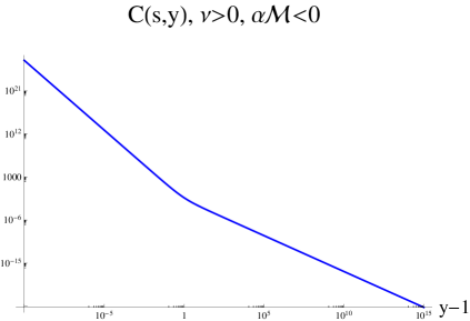
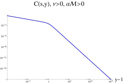
Figure 1: The log-log plots for the correlation functions with positive $\nu$. The parameters $d$ and $s$ do not change the qualitative behaviors, while the parameters $\nu$, actually $L^{2}m^{2}$, and $\alpha\mathcal{M}$ are important for the early time and late time power law scaling.

Positive $\nu$

Let us comment for the case with positive $\nu$. This case has only aging properties if the parameters $\nu$ and $\alpha\mathcal{M}$ are not too large. For $\nu\approx\frac{d+2}{2}$ and $\alpha\mathcal{M}\approx\nu-d-2$, which is allowed by the time boundary condition (88), the bending point, around $\log(y-1)\approx 1$ in the figure 1, sits deep down and the second leg of the plot becomes horizontal. As we increase either $\nu$ or $\alpha\mathcal{M}$, the bending point goes up. This is depicted in the figure 1. For $\alpha=0$ or a particular value of $L^{2}m^{2}$, we can get a straight line, which is identical to the time independent case.

Negative $\nu$

If one is interested in growth phenomena, it is more interesting to consider $\nu<0$. Due to the form of the response function (104), the part $\left(1-1/y\right)^{-\frac{d+2}{2}-\nu}$ determines the properties at early time $y\ll 1$. For $\nu=-\sqrt{\left(1+d/2\right)^{2}+L^{2}m^{2}}$, actually $L^{2}m^{2}$ determines the slope at early time. For $-\left(1+d/2\right)^{2}<L^{2}m^{2}<0$, the slope of the first leg is negative, while that is positive for $L^{2}m^{2}>0$. This can be verified directly in the figure 2.

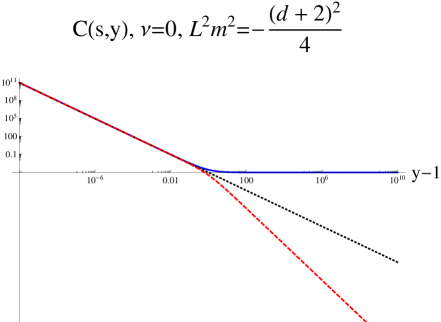
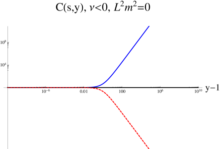
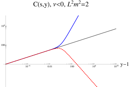
Figure 2: The log-log plots for the correlation functions with negative $\nu$. Each panel has a fixed value of $L^{2}m^{2}$, which determines the slope of the first leg at early time, while the sign of $\alpha\mathcal{M}$ determines the relative slope of the second leg at late time, compared to the first leg. Left : the case saturated with the BF bound $\nu=0$ and $L^{2}m^{2}=-(d+2)^{2}/4$. Three plots are for $\alpha\mathcal{M}=\nu-d-2<0,0,d+2-\nu>0$, which are blue straight, black dotted and red dashed lines, respectively. Similarly for the Middle with $L^{2}m^{2}=0$ and Right plots with $L^{2}m^{2}=2$ with the same values of $\alpha\mathcal{M}=\nu-d-2<0,0,d+2-\nu>0$.

On the other hand, the late time behavior is determined by a factor $y^{-\frac{\alpha\mathcal{M}}{2}-\frac{d+2}{2}-\nu}$. If $\alpha=0$, the slope does not change. The relative slope of the second leg is determined by the sign of $\alpha\mathcal{M}$. This is verified in the figure 2. The real slope of the second leg is governed by the sign of $-\frac{\alpha\mathcal{M}}{2}-\frac{d+2}{2}-\nu$. In particular, early time growth and late time aging happens for

$$L^{2}m^{2}>0\;,\quad\alpha\mathcal{M}>-d-2+\sqrt{\left(d+2\right)^{2}+4L^{2}m^{2}}\;.$$ (105)

The second condition is similar to our time boundary condition (88), but not identical.

4.2 Critical exponents for general $z$ and $d$ : ALCF

For growth phenomena, the roughness of interfaces is quantified by their inter-facial width, $w(l,t)\equiv\langle\sqrt{\langle[h(x,t)-\langle h\rangle_{l}]^{2}\rangle_{l}}$, defined as the standard deviation of the interface height $h(x,t)$ over a length scale $l$ at time $t$ [4]. An equivalent way to describe the roughness is the height-difference correlation function $C(l,t)\equiv\langle[h(x+l,t)-h(x,t)]^{2}\rangle$. $\langle\cdots\rangle_{l}$ and $\langle\cdots\rangle$ denote the average over a segment of length $l$ and all over the interface and ensembles, respectively. Both $w(l,t)$ and $C(l,t)^{1/2}$ are common quantities for characterizing the roughness, for which the so-called Family-Vicsek scaling [54] is expected to hold. The dynamical scaling property is

$$C(l,t)^{1/2}\sim t^{\mathrm{b}}F(lt^{-1/z})\sim\left\{\begin{array}[]{ccc}l^{\mathrm{a}}&\text{for}&l\ll l_{*}\\ t^{\mathrm{b}}&\text{for}&l\gg l_{*}\end{array}\right.\;,$$ (108)

with two characteristic exponents: the roughness exponent ${\mathrm{a}}$ and the growth exponent ${\mathrm{b}}$. The dynamical exponent is given by $z=\frac{\mathrm{a}}{\mathrm{b}}$, and the cross over length scale is $l_{*}\sim t^{1/z}$. For an infinite system, the correlation function behaves as $C(l,t)^{1/2}\sim t^{\mathrm{b}}$ at some late time region $t\gg 1$.

From the two-time correlation function in equation (104), we can get the growth exponent

$$\mathrm{b}_{Aging}=-\frac{\alpha\mathcal{M}}{4}-\frac{d+2}{4}-\frac{\nu}{2}\;,$$ (109)

where $\nu=\pm\sqrt{\left(\frac{2+d}{2}\right)^{2}+L^{2}m^{2}}$. Note that the parameters satisfy the condition (88) from the time boundary conditions. We notice that our system size is infinite, and thus it is not simple matter to obtain the corresponding roughness exponent. The dynamical exponent is not fixed in ALCF, even though the differential equation has $z$ dependence, which can be checked in (82).

For KPZ universality class, there is a nontrivial scaling relation between the roughness exponent $\mathrm{a}$ and the dynamical exponent $z$, chapter 6 in [4]

$$\mathrm{a}+z=2\;.$$ (110)

While this relation is remained to be checked in our holographic model, we assume it is valid to make contact with some field theoretical models. Using the relation $z=\frac{\mathrm{a}}{\mathrm{b}}$, we get

$$\mathrm{a}_{Aging}=\frac{2\mathrm{b}_{Aging}}{\mathrm{b}_{Aging}+1}\;,\quad z_{Aging}=\frac{2}{\mathrm{b}_{Aging}+1}\;.$$ (111)

Let us examine these critical exponents against the known case for $d=1$

$$z_{KPZ}=\frac{3}{2}\;,\quad\mathrm{a}_{KPZ}=\frac{1}{2}\;,\quad\mathrm{b}_{KPZ}=\frac{1}{3}\;.$$ (112)

These can be reproduced with the condition

$$\alpha\mathcal{M}+2\nu=-\frac{13}{3}\;,$$ (113)

which can be matched for $L^{2}m^{2}=2.444\cdots$ and $\alpha\mathcal{M}=0$ for negative $\nu$. We choose $\alpha\mathcal{M}=0$ for the simple growth behavior.

4.2.1 Negative $\nu$

There are two independent critical exponents. One particular interesting exponent is the so called growth exponent $\mathrm{b}=-\frac{\alpha\mathcal{M}}{4}-\frac{d+2}{4}-\frac{\nu}{2}$, where $\nu=\pm\sqrt{\left(\frac{2+d}{2}\right)^{2}+L^{2}m^{2}}$. We consider a dual field theory operator with $\nu=-\sqrt{\left(\frac{2+d}{2}\right)^{2}+L^{2}m^{2}}$, $L^{2}m^{2}\ll\left(\frac{2+d}{2}\right)^{2}$. Then by expanding for small $m$, we get

$$\mathrm{b}_{Aging}\approx\frac{L^{2}m^{2}}{2(d+2)}-\frac{\alpha\mathcal{M}}{4}\;.$$ (114)

Using again $\mathrm{a}+z=2$ and the relation $z=\frac{\mathrm{a}}{\mathrm{b}}$, we get

$$\mathrm{a}_{Aging}\approx\frac{\frac{L^{2}m^{2}}{d+2}-\frac{\alpha\mathcal{M}}{2}}{1+\frac{L^{2}m^{2}}{2(d+2)}-\frac{\alpha\mathcal{M}}{4}}\;,\quad z_{Aging}\approx\frac{2}{1+\frac{L^{2}m^{2}}{2(d+2)}-\frac{\alpha\mathcal{M}}{4}}\;.$$ (115)

If we further restrict our attention to the case $\alpha\mathcal{M}=0$ for considering only the growth phenomena, we have the following dependence on the number of spatial dimensions

$$\mathrm{b}_{ALCF}\approx\frac{Z}{d+2}\;,\qquad\mathrm{a}_{ALCF}\approx\frac{2Z}{d+2+Z}\;,\qquad z_{ALCF}\approx 2\frac{d+2}{d+2+Z}\;,$$ (116)

where $Z=\frac{L^{2}m^{2}}{2}$. For $Z=1.222\cdots$, these exponents match (112) for $d=1$. The corresponding roughness exponent is depicted as blue line in the left panel of the figure 3, which is referred as “ALCF”. To compare with other growth models [4], we also depicted the roughness exponents of the Kim-Kosterlitz model $\mathrm{a}_{KK}=\frac{2}{d+3}$ [55] as well as Wolf-Kertész model $\mathrm{a}_{WK}=\frac{1}{d+1}$ [56].

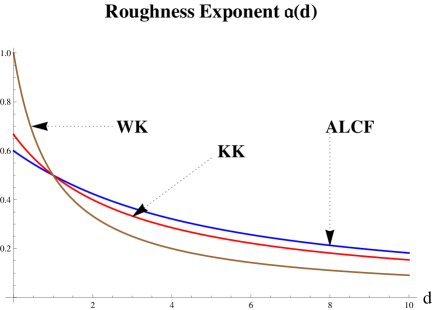
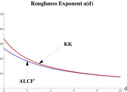
Figure 3: Left panel : plot for the roughness exponent $\mathrm{a}$ of ALCF for $\alpha\mathcal{M}=0$ and $L^{2}m^{2}\approx 2.444\cdots$ that matches KPZ exponents for $d=1$ given in (112). KK represents $\mathrm{a}_{KK}=\frac{2}{d+3}$ from Kim-Kosterlitz [55], while WK $\mathrm{a}_{WK}=\frac{1}{d+1}$ from Wolf-Kertész [56]. Right panel : plot for $\mathrm{a}$ of ALCF^′ for $\alpha\mathcal{M}=0$ and $L^{2}m^{2}=2$ that matches (117) only when $L^{2}m^{2}=2\ll\left(\frac{2+d}{2}\right)^{2}$.

For $Z=1$, we get

$$\mathrm{b}_{ALCF}\approx\frac{1}{d+2}\;,\qquad\mathrm{a}_{ALCF}\approx\frac{2}{d+3}\;,\qquad z_{ALCF}\approx 2\frac{d+2}{d+3}\;,$$ (117)

Our results (117) are only valid for $L^{2}m^{2}=2\ll\left(\frac{2+d}{2}\right)^{2}$, which is referred as “ALCF^′” in the right panel of the figure 3. These exponents have been conjectured for growth in a restricted solid-on-solid model by Kim-Kosterlitz [55][4].

4.3 Response functions with log extensions : ALCF

We have shown in previous sections that the response functions reveal growth and aging behaviors without log or log² corrections. The log and log² corrections have been considered to match further details at early time region [9][10]. In this section, we would like to investigate some more details related to those corrections based on previous results [11].

4.3.1 With log extension

Our two-time response functions with log correction are given by

$$C_{log}(s,y) =s^{-\frac{d+2}{2}-\nu}y^{-\frac{\alpha\mathcal{M}}{2}-\frac{d+2}{2}-\nu}\left(1-\frac{1}{y}\right)^{-\frac{d+2}{2}-\nu}$$

$$\quad\times\bigg{\{}1+R_{1}(\ln s+\ln y)+R_{1}\ln[1-\frac{1}{y}]\bigg{\}}\;,$$ (118)

where $s=t_{1}$, $y=\frac{t_{2}}{t_{1}}$, $\nu$ and $\alpha\mathcal{M}$ are free parameters, while the coefficients are given by

$$R_{1}=\frac{\nu}{1-\nu\psi(\nu)+\nu\ln[\mathcal{M}_{B}]}\;.$$ (119)

We note that the coefficients are completely fixed by two fixed parameters

$$\mathcal{M}_{B}=\frac{\mathcal{M}u_{B}^{2}}{2}\;,\qquad\psi(\nu)=\frac{\Gamma(\nu)^{\prime}}{\Gamma(\nu)}\;.$$ (120)

Note that similar result for $z=2$ and $d=2$ has been available in [11]. The detailed comparisons between (4.3.1) and the phenomenological field theory model [9][10] were investigated. We noted that the terms proportional to $\ln s$ and $\ln y$ are not considered in [9][10], which do not modify qualitative features of the response functions. For this case, the analysis done in [11] is still valid.

4.3.2 With log² extension

We obtain the log² extension of the response function using holographic approach

$$C_{log^{2}}(s,y)=s^{-\frac{d+2}{2}-\nu}y^{-\frac{\alpha\mathcal{M}}{2}-\frac{d+2}{2}-\nu}\left(1-\frac{1}{y}\right)^{-\frac{d+2}{2}-\nu}$$

$$\qquad\qquad\quad\times\bigg{\{}1+\tilde{R}_{1}(\ln s+\ln y)+\tilde{R}_{2}(\ln s+\ln y)^{2}\bigg{.}$$

$$\qquad\qquad\qquad\bigg{.}+[\tilde{R}_{1}+2\tilde{R}_{2}(\ln s+\ln y)]\ln[1-\frac{1}{y}]+\tilde{R}_{2}\ln[1-\frac{1}{y}]^{2}\bigg{\}}\;,$$ (121)

where

$$\tilde{R}_{1}=-\frac{\tilde{A}_{1}+2\tilde{A}_{2}\ln[\mathcal{M}_{B}]}{\tilde{A}_{0}+\tilde{A}_{1}\ln[\mathcal{M}_{B}]+\tilde{A}_{2}\ln[\mathcal{M}_{B}]^{2}}\;,$$ (122)

$$\tilde{R}_{2}=\frac{\tilde{A}_{2}}{\tilde{A}_{0}+\tilde{A}_{1}\ln[\mathcal{M}_{B}]+\tilde{A}_{2}\ln[\mathcal{M}_{B}]^{2}}\;,$$ (123)

$$\tilde{A}_{0}=1+\nu\psi-\nu^{2}(\psi^{2}-\psi^{\prime})\;,$$ (124)

$$\tilde{A}_{1}=(2\nu^{2}\psi-\nu)\;,\qquad\tilde{A}_{2}=-\nu^{2}\;.$$ (125)

These coefficients are also completely fixed by two fixed parameters given in (120). Compared to $C(s,y)$, a new parameter $\mathcal{M}_{B}$ determines the behaviors of response functions related to the log and log² contributions. As we explicitly check in the figure 4, the qualitative behavior of the response functions does not change with the log and log² contributions for reasonably small $\mathcal{M}_{B}$. The growth exponent and aging properties are determined by the two parameters $L^{2}m^{2}$ and $\alpha\mathcal{M}$, which define our theory.

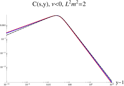
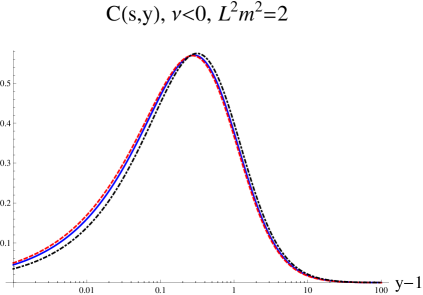
Figure 4: Plots for $C(s,y)$ with blue straight, $C_{log}(s,y)$ with red dashed and $C_{log^{2}}(s,y)$ with black dot-dashed lines for $\nu<0$, $d=1$, $s=4$ and $L^{2}m^{2}=2$. For the response functions with log corrections, we need one more input $\mathcal{M}_{B}$, which we took $\mathcal{M}_{B}=10^{-15}$ for these plots. The smaller the value of $\mathcal{M}_{B}$, the smaller the differences between $C(s,y)$ and its log extensions.

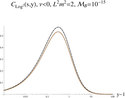
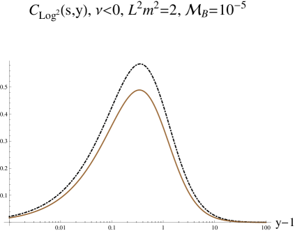
Figure 5: Plots for $C_{Log^{2}}(s,y)$ with black dot-dashed and $C_{Log^{2}}^{Wanted}(s,y)$ with brown straight lines for $\nu<0$, $d=1$, $s=4$ and $L^{2}m^{2}=2$. Left : $\mathcal{M}_{B}=10^{-15}$, Right : $\mathcal{M}_{B}=10^{-5}$. We check that there is no qualitative changes due to the unwanted terms explained in (4.3.2).

We would like to compare our results (4.3.2) with the following equation, which is equation (10) of [9] (or equation (4.3) of [10]), obtained from the phenomenological field theory model.

$$R(s,y) =s^{-1-a}y^{-\lambda_{R}/z}\left(1-\frac{1}{y}\right)^{-1-a^{\prime}}$$ (126)

$$\times\left(h_{0}-g_{12,0}\tilde{\xi}^{\prime}\ln[1-\frac{1}{y}]-\frac{1}{2}f_{0}\tilde{\xi}^{\prime 2}\ln^{2}[1-\frac{1}{y}]-g_{21,0}\xi^{\prime}\ln[y-1]+\frac{1}{2}f_{0}\xi^{\prime 2}\ln^{2}[y-1]\right)\;,$$

where the parameters $g_{12,0},g_{21,0},\tilde{\xi}^{\prime},\xi^{\prime},f_{0}$ come from the logarithmic extension in the field theory side. From the phenomenological input [10] “the parenthesis becomes essentially constant for sufficiently large $y$,” the condition $\xi^{\prime}=0$ is imposed to remove the last two terms. The other parameters in (126) are determined to match available data. We can identify the exponents $a,a^{\prime},\lambda_{R}$ by comparing the equation to our result [11]

$$\nu=a-1=a^{\prime}-1\;,\qquad\frac{\alpha\mathcal{M}}{2}=\frac{\lambda_{R}}{z}-1-a\;.$$ (127)

By including the log² corrections, we provide the necessary terms $\tilde{R}_{2}\ln[1-\frac{1}{y}]^{2}$ as well as $\tilde{R}_{1}\ln[1-\frac{1}{y}]$. The relative coefficients between them are fixed by (122). On the other hand, there exist also several unwanted terms inside the parenthesis of (4.3.2). First, we note new terms $\tilde{R}_{2}(\ln s+\ln y)^{2}$ and $2\tilde{R}_{2}(\ln s+\ln y)\ln[1-\frac{1}{y}]$ due to log² corrections, in addition to $\tilde{R}_{1}(\ln s+\ln y)$ coming from the log correction. All these terms might spoil the desired properties of the phenomenological response function (126). To examine the effects coming from these unwanted terms, we plot the response function with only wanted terms as

$$C_{log^{2}}^{Wanted}(s,y) =s^{-\frac{d+2}{2}-\nu}y^{-\frac{\alpha\mathcal{M}}{2}-\frac{d+2}{2}-\nu}\left(1-\frac{1}{y}\right)^{-\frac{d+2}{2}-\nu}$$

$$\quad\times\bigg{\{}1+\tilde{R}_{1}\ln[1-\frac{1}{y}]+\tilde{R}_{2}\ln[1-\frac{1}{y}]^{2}\bigg{\}}\;.$$ (128)

We explicitly check in the figure 5 that the full response functions (4.3.2) have a qualitatively similar behavior compared to those (4.3.2) with only wanted terms in the field theory approach.

4.4 Critical exponents for $z=\frac{3}{2}$ and $d=1$ : Aging backgrounds

While the dynamical exponent $z$ for the ALCF is not fixed in obtaining the correlation and response functions, those of the Schrödinger backgrounds crucially depend on $z$. In fact, obtaining analytic solutions of the differential equation (59) is a highly non-trivial task. Fortunately, we are able to get response functions for $z=\frac{3}{2}$ with some approximations as

$$C_{Schr}(s,y)=s^{-\frac{d+2}{2}-f\nu}y^{-\frac{\alpha\mathcal{M}}{2}-\frac{d+2}{2}-f\nu}\left(1-\frac{1}{y}\right)^{-\frac{d+2}{2}-f\nu}\;,$$ (129)

where $s=t_{1}$, $y=\frac{t_{2}}{t_{1}}$, $\nu$ and $\alpha\mathcal{M}$ are free parameters. This is valid for the Aging background (96) as well as the Schrödinger background, $\alpha=0$, given by (66) with $f=1$ for $\mathcal{M}\rightarrow 0$ and by (72) with $f=2$ for $\mathcal{M}\rightarrow\infty$.

From the two-time response functions in equation (104), we can get the growth exponent

$$\mathrm{b}_{Aging}^{f}=-\frac{\alpha\mathcal{M}}{4}-\frac{d+2}{4}-\frac{f\nu}{2}\;,$$ (130)

where $\nu=\pm\sqrt{\left(\frac{2+d}{2}\right)^{2}+L^{2}m^{2}}$. Now the dynamical exponent is fixed as $z=\frac{3}{2}$ for the aging background. Using the relation $z=\frac{\mathrm{a}}{\mathrm{b}}$, we get

$$\mathrm{a}^{f}_{Aging}=\frac{3\mathrm{b}_{Aging}}{2}=-\frac{3\alpha\mathcal{M}}{8}-\frac{3(d+2)}{8}-\frac{3f\nu}{4}\;.$$ (131)

The critical exponents for the KPZ universality class given in (112) can be reproduced with the condition

$$\alpha\mathcal{M}+2f\nu=-\frac{13}{3}\;,$$ (132)

which can be matched for $\alpha\mathcal{M}\approx 0$ and $L^{2}m^{2}\approx\left(\frac{13}{6f}\right)^{2}-\frac{9}{4}$ for negative $\nu$. The value of $L^{2}m^{2}$ for $f=2$ becomes negative, yet is allowed as we can see from the expression of $\nu$.

5 Conclusion

We have extended our geometric realizations of aging symmetry in several different ways based on previous works for $z=2$ and $d=2$ [11][13]. First, we generalize our correlation and response functions to the non-conformal setup with general dynamical exponent $z$ and for arbitrary spatial dimensions $d$. They have Galilean symmetries with time translation symmetry, which are summarized in the equations (14), (66) and (72). For convenience, we reproduce equation (14) here

$$\langle\phi^{*}(x_{2})\phi(x_{1})\rangle=\frac{\Gamma(1-\nu)}{\Gamma(\nu)\Gamma(-\nu)}\frac{L^{d+1}\mathcal{M}^{\frac{d}{2}+\nu}}{\pi 2^{\nu-1}u_{B}^{d+2-2\nu}}\cdot\frac{\theta(t_{2})\theta(t_{2}-t_{1})}{(t_{2}-t_{1})^{\frac{d+2}{2}+\nu}}\cdot\exp\left(-{\frac{\mathcal{M}(\vec{x}_{2}-\vec{x}_{1})^{2}}{2(t_{2}-t_{1})}}\right)\;,$$ (133)

which is valid for general $z$ and $d$. Second, these are extended with log and log² corrections with appropriate bulk actions. Practically, these corrections can be computed using simple properties of the differential operators (18), (60) and their commutation relations (23). The results are listed in (2.1.2), (52) for ALCF, (68), (69) for Schrödinger backgrounds. All these response functions have time translation invariance.

Third, on top of these extensions, we also compute response functions with aging symmetry, by breaking the global time translation invariance using a singular coordinate transformation (80). We check the general relation between the aging response functions and those of Schrödinger backgrounds holds (97)

$$\langle\phi^{*}(x_{2})\phi(x_{1})\rangle_{Aging}^{z,d}=\left(\frac{t_{2}}{t_{1}}\right)^{-\frac{\alpha\mathcal{M}}{2}}\langle\phi^{*}(x_{2})\phi(x_{1})\rangle_{Schr}^{z,d}\;.$$ (134)

This generalization is independent of the logarithmic extensions.

With these results, we investigate our two-time response functions for general $z$ and especially for arbitrary number of spatial dimensions $d$ with log and log² extensions (4.3.2)

$$C(s,y)=s^{-\frac{d+2}{2}-\nu}y^{-\frac{\alpha\mathcal{M}}{2}-\frac{d+2}{2}-\nu}\left(1-\frac{1}{y}\right)^{-\frac{d+2}{2}-\nu}\bigg{\{}1+\cdots\bigg{\}}\;,$$ (135)

where $\cdots$ represent various contributions from the log and log² extensions. From the systematic analysis, we have found that our two-time response functions reveal a power-law scaling behavior at early time region, which is distinct from another power-law scaling at late time region. This can be explicitly checked in the figure 2. The early time power scaling behaviors are governed by the scaling dimensions of the dual field theory operators. In particular, their growth and aging is determined by the sign of the parameter $L^{2}m^{2}$. The late time behaviors are modified by $\alpha\mathcal{M}$, the aging parameter. If $\alpha=0$, the initial behaviors persist without change, which is expected due to its time translation invariance. The turning point between these two time regions is marked by the waiting time $s=t_{1}$. The log and log² corrections provide further modifications that would match detailed data by turning available parameters.

Let us conclude with some observations and future directions toward holographic realizations of KPZ universality class. Our generalizations of the holographic response functions to general $z$ and $d$ open up some possibilities to have contact with the higher dimensional growth and aging phenomena. We have done the first attempt to do so in §4.2. We make some contacts with Kim-Kosterlitz model [55] at higher spatial dimensions with an assumptions (110) for some particular dual scalar operators. Although it is not perfect, we consider this as a promising sign for the future developments along the line.

We mention two pressing questions we would like to answer in a near future. Our holographic model is an infinite system, and thus obtaining the roughness exponent “$\mathrm{a}$” is rather challenging. Progresses on this point will provide a big step toward realizing holographic KPZ class. Assumption (110) is well understood in the field theoretical models [4]. There Galilean invariance was a crucial ingredient, which is also important in our holographic model. Verifying this relation would be an important future challenge.

References

[1]
[2]
M. Henkel, H. Hinrichsen and S. Lübeck,
“Non-equilibrium phase transitions vol. 1 : absorbing phase transitions,”
Springer (Heidelberg 2009).
[3]
M. Henkel and M. Pleimling,
“Non-equilibrium phase transitions vol. 2 : ageing and dynamical scaling far from equilibrium,”
Springer (Heidelberg 2010).
[4]
A. L. Barabási and H. E. Stanley,
“Fractal concepts in surface growth,”
Cambridge University Press (1995).
[5]
H. Hinrichsen,
“Nonequilibrium Critical Phenomena and Phase Transitions into Absorbing States,”
Adv. Phys. 49, 815 (2000)
[arXiv:cond-mat/0001070].
[6]
M. Kardar, G. Parisi and Y.-C. Zhang,
“Dynamic Scaling of Growing Interfaces,”
Phys. Rev. Lett. 56, 889 (1986).
[7]
K. Takeuchi, M. Sano,
“Universal Fluctuations of Growing Interfaces: Evidence in Turbulent Liquid Crystals,”
Phys. Rev. Lett. 104, 230601 (2010).
[arXiv:1001.5121][cond-mat.stat-mech].
[8]
K. Takeuchi, M. Sano, T. Sasamoto and H. Spohn,
“Growing interfaces uncover universal fluctuations behind scale invariance,”
Sci. Rep. 1, 34
[arXiv:1108.2118][cond-mat.stat-mech].
[9]
M. Henkel, J. D. Noh and M. Pleimling,
“Phenomenology of ageing in the Kardar-Parisi-Zhang equation,”
Phys. Rev. E 85, 030102(R) (2012)
[arXiv:1109.5022][cond-mat.stat-mech].
[10]
M. Henkel,
“On logarithmic extensions of local scale-invariance,”
Nucl. Phys. B 869, 282 (2013)
[arXiv:1009.4139][hep-th].
[11]
S. Hyun, J. Jeong and B. S. Kim,
“Aging Logarithmic Conformal Field Theory : a holographic view,”
JHEP 1301, 141 (2013)
[arXiv:1209.2417][hep-th].
[12]
J. I. Jottar, R. G. Leigh, D. Minic and L. A. Pando Zayas,
“Aging and Holography,”
JHEP 1011, 034 (2010)
[arXiv:1004.3752][hep-th].
[13]
S. Hyun, J. Jeong and B. S. Kim,
“Finite Temperature Aging Holography,”
JHEP 1203, 010 (2012)
[arXiv:1108.5549][hep-th].
[14]
J. M. Maldacena,
“The large N limit of superconformal field theories and supergravity,”
Adv. Theor. Math. Phys. 2, 231 (1998)
[Int. J. Theor. Phys. 38, 1113 (1999)]
[arXiv:hep-th/9711200].
[15]
O. Aharony, S. S. Gubser, J. M. Maldacena, H. Ooguri and Y. Oz,
“Large N field theories, string theory and gravity,”
Phys. Rept. 323, 183 (2000)
[arXiv:hep-th/9905111].
[16]
M. Flohr,
“Bits and pieces in logarithmic conformal field theory,”
Int. J. Mod. Phys. A 18, 4497 (2003)
[arXiv:hep-th/0111228].
[17]
M. R. Gaberdiel,
“An algebraic approach to logarithmic conformal field theory,”
Int. J. Mod. Phys. A 18, 4593 (2003)
[arXiv:hep-th/0111260].
[18]
A. M. Ghezelbash, M. Khorrami and A. Aghamohammadi,