Effect of sine-Gaussian glitches on searches for binary coalescence

Abstract

We investigate the effect of an important class of glitches occurring in the detector data on matched filter searches of gravitational waves from coalescing compact binaries in the advanced detector era. The glitches, which can be modeled as sine-Gaussians, can produce triggers with significant time delays and thus have important bearing on veto procedures as will be described in the paper. We provide approximated analytical estimates of the trigger SNR and time as a function of the parameters describing the sine-Gaussian (center time, center frequency and $Q$-factor) and the inspiral filter (chirp mass). We validate our analytical predictions through simple numerical simulations, performed by filtering noiseless sine-Gaussians with the inspiral matched filter and recovering the time and value of the maximum of the resulting SNR time series. Although we identify regions of the parameter space in which each approximation no longer reproduces the numerical results, the approximations complement each other and together effectively cover the whole parameter space.

1 Introduction

Advanced interferometric gravitational-wave detectors are currently under construction and are expected to start delivering strain data in a few years. Major improvements over the first-generation interferometers will include a significantly better sensitivity curve at all frequencies of interest, which will effectively shift the sensitive band lower boundary from $\sim 40$ Hz to $\sim 10$ Hz [1, 2].

A promising source of gravitational-wave detections in the advanced interferometer era is represented by the inspiral and coalescence of compact binary systems, such as binary neutron stars (BNS), binary black holes and black hole-neutron star binaries [3]. The strain waveform associated with such events can be calculated to a good approximation at least for some regions of the parameter space describing the binary system [4]. Consequently, the classical data analysis pipeline for detecting such signals employs a filter matched to the analytical waveform [5]. This approach consists in correlating the strain data with the waveform and producing an estimate of the signal to noise ratio (SNR) for that waveform. Triggers are then generated whenever the SNR exceeds a pre-defined threshold. Lists of triggers are independently produced for each detector and combined to obtain coincident triggers, which are then checked for consistency and passed on to more elaborate analysis. Similar search pipelines will be employed in the advanced detector era. However, in order to exploit the improved noise curves and extend the search to lower frequencies, the strain data will have to be filtered with significantly longer inspiral waveforms than used for past searches (up to tens of minutes as opposed to about one minute for BNS). In fact, the duration of the waveform in the interferometer output depends strongly on the low-frequency cutoff [6].

First generation interferometers were affected by high rates of short-duration transients unrelated to astrophysical events and commonly known as glitches, most of which can be roughly modeled as short sine-Gaussian waveforms with a few cycles, i.e. a small $Q$-factor [7]. The typical effect of glitches on searches for binary coalescence is a significant deviation of the SNR distribution from what expected for stationary Gaussian noise, i.e. an exponential distribution. In particular, glitches produce tails of high-SNR outliers unrelated to astrophysical signals. This increases the false-alarm rate of the search and lowers our confidence on possible detections of true inspiral signals (see [8], figure 8). In past searches, most glitches were ruled out as gravitational-wave candidates by monitoring auxiliary channels and their origin could rather be attributed either to the noisy environment of the detector (for instance seismic noise, weather, electromagnetic disturbances) or to unexpected behavior of the detector itself (saturation of analog-to-digital converters, problems with control systems and thermal compensation, scattered light) [9]. Nevertheless, surviving glitches still increased the rate of coincident triggers between detectors and thus weakened our ability to both confidently detect signals as well as set strong upper limits on the coalescence rate. Unfortunately, despite the improved sensitivity, advanced detectors are expected to manifest similar glitches in their output. This will still pose significant challenges to future gravitational-wave searches and could in fact be their ultimate limiting factor. Hence, studies investigating the effect of data quality on searches play a central role in future results.

A potential complication of advanced inspiral searches is the fact that the longer BNS inspiral filters could lead to significant time delays between the occurrence of a short, isolated glitch and the coalescence time of the resulting spurious inspiral trigger. Often, such delays will be much longer than the glitch itself and they may have an impact both on existing veto procedures based on auxiliary channels and on the tuning of consistency checks such as Allen’s $\chi^{2}$ [10], bank $\chi^{2}$ and auto $\chi^{2}$ [11]. Being able to predict the parameters of spurious inspiral triggers produced by glitches is important for understanding such issues and could hint at new veto techniques for reducing false-alarms produced by glitches.

For this reason, we study the effect of glitches with sine-Gaussian waveform on a matched-filter search for inspiral gravitational waves in the advanced detector era. We present approximations to the complex matched-filter output and to the SNR time series (the quantity used for producing the inspiral triggers) for the case where the signal is just a noiseless sine-Gaussian with no additional signal components on top of it. Given the parameters of the glitch model (central time $t_{0}$, central frequency $f_{0}$ and quality factor $Q$) such approximations allow one to predict the SNR and time of the resulting spurious triggers as a function of the chirp mass $\mathcal{M}$ of each template. We present three such approximations which complement each other and completely cover the parameter space of the sine-Gaussians. We support the approximations with numerical simulations.

The paper is organized as follows. In section 2 we briefly review the matched filter algorithm and fix the relevant notation. In section 3 we derive the approximated estimates for the SNR time series and trigger parameters. In section 4 we compare these results to numerical simulations and we identify regimes where the different approximations are no longer acceptable. Section 5 discusses the implications of our results and suggests a way to use such results for constructing a veto procedure for the advanced era.

2 Matched filter

A matched filter search combines a detector strain data segment $s$, the signal to be sought $h$ and the one-sided power spectral density (PSD) of the detector noise $S_{\rm n}(f)$ into a quantity representing the SNR as a function of the parameters describing the gravitational-wave source [6]. The SNR for a binary coalescing at time $t_{\rm c}$ is calculated as

$$\rho(t_{\rm c})=\frac{|z(t_{\rm c})|}{\sigma}$$ (1)

where $z(t_{\rm c})$ is the output of the complex matched filter,

$$z(t_{\rm c})=4\int_{f_{\rm L}}^{f_{\rm H}}\frac{\tilde{s}(f)\tilde{h}^{*}(f;t_{\rm c})}{S_{\rm n}(f)}\rmd f$$ (2)

and $\sigma$ is the sensitivity of the detector to the sought after signal,

$$\sigma^{2}=4\int_{f_{\rm L}}^{f_{\rm H}}\frac{|\tilde{h}(f;t_{\rm c})|^{2}}{S_{\rm n}(f)}\rmd f.$$ (3)

In the above expressions, $\tilde{s}(f)$ is the Fourier transform of the pre-conditioned data segment and

$$\tilde{h}(f;t_{\rm c})=h_{0}f^{-7/6}e^{-i\psi(f;t_{\rm c})}$$ (4)

is the inspiral signal template expressed in the frequency domain via the stationary phase approximation [12]. $f_{\rm L}$ and $f_{\rm H}$ are frequency cutoff values. Searches performed on first-generation detector data used $f_{\rm L}=40$ Hz and for advanced interferometers $f_{\rm L}=10$ Hz is expected. $f_{\rm H}$ is usually set to the frequency corresponding to the innermost stable circular orbit of a test mass orbiting a Schwarzschild black hole, i.e. $f_{\rm ISCO}=c^{3}/(6\sqrt{6}\pi GM)$.

Candidate inspiral triggers are identified as local maxima of the SNR crossing a pre-established threshold. Each trigger carries the set of associated parameter values, e.g. coalescence time and phase and binary component masses.

3 Response to a sine-Gaussian waveform

We are interested in calculating the response of the inspiral matched filter to a sine-Gaussian waveform, i.e. the SNR time series $\rho(t_{\rm c})$ after the center time of the sine-Gaussian. From $\rho(t_{\rm c})$ we then want to estimate the maximum SNR $\hat{\rho}$ and the corresponding time $\hat{t}_{\rm c}$. The signal we consider includes only a sine-Gaussian glitch: neither the stochastic noise of the detector nor any kind of astrophysical gravitational wave signals are added. Therefore, our results will represent averages over the ensemble of noise realizations. They will also not describe the case of a glitch contaminating a true inspiral signal.

The sine-Gaussian waveform can be written in the time domain as

$$s(t)=A\exp\left(-\frac{(t-t_{0})^{2}}{\tau^{2}}\right)\cos(2\pi f_{0}t+\phi_{0})$$ (5)

where $A$ is an overall amplitude, $t_{0}$ and $f_{0}$ are the location of the sine-Gaussian in time and frequency respectively, $\tau=Q/2\pi f_{0}$ is the time duration, $Q$ is the dimensionless quality factor and $\phi_{0}$ is the phase of the oscillation at $t=0$. We are free to define the time origin as $t_{0}=0$, so that $\hat{t}$ represents the time delay between the sine-Gaussian and the inspiral trigger. Since the SNR is linear in the signal amplitude, we can also set $A=1$. The sine-Gaussian can then be expressed in the frequency domain as

$$\tilde{s}(f)=\frac{\sqrt{\pi}}{2}\tau\exp\left(-\pi^{2}\tau^{2}(f-f_{0})^{2}+i\phi_{0}\right)\left[1+\exp\left(-Q^{2}\frac{f}{f_{0}}-2i\phi_{0}\right)\right].$$ (6)

For $f_{\rm L}<f<f_{\rm H}$, the second exponential falls off very quickly as $Q$ increases from 1, so we neglect it altogether. We can now also set $\phi_{0}=0$ since the SNR is not affected by global phase factors. Inserting (4) and the so-modified (6) into (2) we get

$$z(t_{\rm c})=2\sqrt{\pi}\tau h_{0}\int_{f_{\rm L}}^{f_{\rm H}}\frac{f^{-7/6}}{S_{\rm n}(f)}\exp\left(-\pi^{2}\tau^{2}(f-f_{0})^{2}+i\psi(f;t_{\rm c})\right)\rmd f.$$ (7)

In order to get an explicit expression, we approximate $\psi(f;t_{\rm c})$ with the simple Newtonian chirp [13]

$$\psi(f;t_{\rm c})=2\pi ft_{\rm c}-2\phi-\frac{\pi}{4}+\frac{3}{128}(\zeta f)^{-5/3}$$ (8)

where $t_{\rm c}$ is the coalescence time, $\phi$ is the orbital phase at coalescence, $\zeta=\pi G\mathcal{M}/c^{3}$ and $\mathcal{M}=(m_{1}m_{2})^{3/5}/(m_{1}+m_{2})^{1/5}$ is the chirp mass of the binary system composed of masses $m_{1}$ and $m_{2}$. Although the resulting integral can not be evaluated exactly, different approximations can be found, as will be discussed in the next subsections.

3.1 Approximation I

The first approximation we describe makes use of the stationary phase approximation. If $\rmd\psi/\rmd f=0$ at a frequency $f_{\rm s}$, we can approximate $\psi(f;t_{\rm c})$ around $f_{\rm s}$ with a second order power series,

$$\psi(f;t_{\rm c})\approx\psi(f_{\rm s})+\beta(f-f_{\rm s})^{2}$$ (9)

For the Newtonian chirp this holds and we have

$$f_{\rm s} = \left(\frac{5}{256\pi}\right)^{3/8}\zeta^{-5/8}t_{\rm c}^{-3/8}=f_{0}\left(\frac{\tau_{0}}{t_{\rm c}}\right)^{3/8}$$ (10)

$$\beta = \frac{5}{96}f_{\rm s}^{-11/3}\zeta^{-5/3}$$ (11)

where $\tau_{0}$ is the first chirp time evaluated using $f_{0}$ as the fiducial frequency [14]. Note that $f_{\rm s}$ is a function of the coalescence time and we are evaluating a family of integrals parametrized by $t_{\rm c}$. The factor $f^{-7/6}S_{\rm n}^{-1}(f)$ in (7) varies more slowly with frequency than the exponential, so we take it as constant and evaluate it at $f_{\rm s}$. The integrand can then be rewritten as the product of two Gaussians, one real and one complex, so the matched filter output is (omitting irrelevant phase factors)

$$z(t_{\rm c})\approx 2\sqrt{\pi}\tau\frac{f_{\rm s}^{-7/6}}{S_{\rm n}(f_{\rm s})}\int_{f_{\rm L}}^{f_{\rm H}}\exp\left(i\frac{(f-f_{\rm s})^{2}}{2\sigma^{2}_{\rm f}}-\frac{(f-f_{0})^{2}}{2\sigma^{2}_{\rm sg}}\right)\rmd f$$ (12)

where $\sigma_{\rm sg}=1/\sqrt{2}\pi\tau$ and $\sigma_{\rm f}=\sqrt{3f_{0}/16\pi\tau_{0}}(f_{\rm s}/f_{0})^{11/6}$ are the standard deviations of the Gaussians. Using (12) and (3) in (1), and carrying out the integral using Cauchy’s theorem, we get

$$\rho(t_{\rm c})\approx\frac{1}{\sigma_{0}}\frac{\exp\left(-\frac{(f_{0}-f_{\rm s})^{2}}{2\sigma^{2}_{\rm f}}\frac{\sigma_{\rm sg}^{2}/\sigma_{\rm f}^{2}}{1+\sigma_{\rm sg}^{4}/\sigma_{\rm f}^{4}}\right)}{f_{\rm s}^{7/6}S_{\rm n}(f_{\rm s})(1+\sigma_{\rm sg}^{4}/\sigma_{\rm f}^{4})^{1/4}}$$ (13)

with $\sigma_{0}^{2}=\int_{0}^{\infty}f^{-7/3}S_{\rm n}^{-1}(f)\rmd f$.

This is a complicated function of $t_{\rm c}$ through $f_{\rm s}$ and $\sigma_{\rm f}$. In particular note that $t_{\rm c}$ also enters via $S_{\rm n}(f_{\rm s})$ and so the shape of the SNR pulse in time depends on the PSD of the noise. Although $S_{\rm n}(f)$ can in principle be modeled as a combination of power laws, the resulting expression is complicated and a numerical maximization is thus needed in order to determine $\hat{\rho}$ and $\hat{t}_{\rm c}$.

3.2 Approximation II

Our second method is a slightly different application of the stationary phase approximation and is expected to be appropriate for small $Q$. In fact, we still use (9) but we now assume that the largest contribution to the integral in (7) comes from a narrow band around $f_{\rm s}$. Within this band, we can thus consider all other terms of the integrand constant and equal to their value at $f_{\rm s}$, including the sine-Gaussian peak, so the integral reduces to

$$\int_{f_{\rm L}}^{f_{\rm H}}e^{i\beta(f-f_{\rm s})^{2}}\rmd f\approx\sqrt{\frac{\pi}{\beta}}.$$ (14)

Therefore, omitting all irrelevant phase terms,

$$z(t_{\rm c})\approx 2\pi\tau h_{0}\frac{\exp\left(-\pi^{2}\tau^{2}(f_{\rm s}-f_{0})^{2}\right)}{f_{\rm s}^{7/6}S_{\rm n}(f_{\rm s})\beta^{1/2}}$$ (15)

and the resulting SNR time series is

$$\rho(t_{\rm c})\approx\frac{\pi\tau}{\sigma_{0}}\frac{\exp\left(-\pi^{2}\tau^{2}(f_{\rm s}-f_{0})^{2}\right)}{f_{\rm s}^{7/6}S_{\rm n}(f_{\rm s})\beta^{1/2}}.$$ (16)

For the Newtonian chirp,

$$\rho(t_{\rm c})\approx\frac{\sqrt{6}\pi^{3/4}}{5^{1/4}}\frac{\tau\zeta^{5/12}}{\sigma_{0}}\frac{\exp\left(-\pi^{2}\tau^{2}(f_{\rm s}-f_{0})^{2}\right)}{S_{\rm n}(f_{\rm s})}t_{\rm c}^{-1/4}.$$ (17)

This is still a quite complicated function of time and it still depends on the PSD of the noise. In general, at least for a smooth PSD with no peaks, it is the product of two peaks with different time scales, one corresponding to the exponential term and the other associated with the $f_{\rm s}^{7/6}S_{\rm n}(f_{\rm s})\beta^{1/2}$ term. Thus $\hat{t}_{\rm c}$ depends on $f_{0}$, $\tau$, $\zeta$ and the details of $S_{\rm n}(f)$ even for the Newtonian chirp. Although we expect approximation II to be valid for small $Q$, we can try to take the result to the limit of $Q\to\infty$. The exponential becomes more peaked than the $f_{\rm s}^{-7/6}S_{\rm n}^{-1}(f_{\rm s})\beta^{-1/2}$ term, so $\rho(t_{\rm c})$ is maximum where $f_{\rm s}=f_{0}$ and

$$\hat{\rho} \approx\frac{\pi\tau}{\sigma_{0}}f_{0}^{-7/6}S_{\rm n}^{-1}(f_{0})\beta^{-1/2}$$ (18)

$$\hat{t}_{\rm c} \approx\tau_{0}.$$ (19)

This suggests that in the large $Q$ limit the trigger delay is just the time the inspiral takes to coalesce after crossing the center frequency of the sine-Gaussian, which can be expected from intuition. As we said, however, this approximation is expected to work for small $Q$ and thus in general $\hat{\rho}$ and $\hat{t}_{\rm c}$ must be found numerically.

3.3 Approximation III

Although probably less useful in practice, a different approximation can be derived in the large $Q$ limit. In this regime the integrand in (7) is no longer dominated by the band around $f_{\rm s}$ but by the narrow peak of the sine-Gaussian, centered on $f_{0}$. Again, the factor $f^{-7/6}S_{\rm n}^{-1}(f)$ varies slowly with frequency and can be regarded as constant, and the integral limits can be extended over the real axis. We still approximate the template phase as a second-order Taylor series, but this time around $f_{0}$,

$$\psi(f;t_{\rm c})\approx\psi(f_{0})+\alpha(f-f_{0})+\beta(f-f_{0})^{2}.$$ (20)

For instance, for the Newtonian chirp we have

$$\alpha = 2\pi t_{\rm c}-\frac{5}{128}f_{0}^{-8/3}\zeta^{-5/3}=2\pi(t_{\rm c}-\tau_{0})$$ (21)

$$\beta = \frac{5}{96}f_{0}^{-11/3}\zeta^{-5/3}.$$ (22)

After switching the integration variable to $x=\sqrt{\pi^{2}\tau^{2}-i\beta}(f-f_{0})$, and omitting irrelevant phase factors, we are left with a Gaussian integral

$$z(t_{\rm c})\approx\frac{2\sqrt{\pi}\tau h_{0}}{\sqrt{\pi^{2}\tau^{2}-i\beta}}\frac{f_{0}^{-7/6}}{S_{\rm n}(f_{0})}\int_{-\infty}^{+\infty}\exp\left(-x^{2}+\frac{i\alpha x}{\sqrt{\pi^{2}\tau^{2}-i\beta}}\right)\rmd x$$ (23)

which readily gives

$$z(t_{\rm c})\approx\frac{2\pi\tau h_{0}}{\sqrt{\pi^{2}\tau^{2}-i\beta}}\frac{f_{0}^{-7/6}}{S_{\rm n}(f_{0})}\exp\left(-\frac{\alpha^{2}}{4(\pi^{2}\tau^{2}-i\beta)}\right).$$ (24)

The final expression for the approximated SNR time series is

$$\rho(t_{\rm c})\approx\frac{1}{\sigma_{0}}\frac{\exp\left(-\alpha^{2}/4\pi^{2}\tau^{2}(1+\frac{\beta^{2}}{\pi^{4}\tau^{4}})\right)}{f_{0}^{7/6}S_{\rm n}(f_{0})\left(1+\frac{\beta^{2}}{\pi^{4}\tau^{4}}\right)^{1/4}}.$$ (25)

In the case of the Newtonian chirp $\alpha$ is the only function of $t_{\rm c}$, so $\rho(t_{\rm c})$ is a simple Gaussian pulse and we obtain explicit expressions for trigger SNR and time,

$$\hat{\rho} \approx\sigma^{-1}_{0}f_{0}^{-7/6}S_{\rm n}^{-1}(f_{0})\left(1+\frac{\beta^{2}}{\pi^{4}\tau^{4}}\right)^{-1/4}$$ (26)

$$\hat{t}_{\rm c} \approx\tau_{0}.$$ (27)

Note that $\hat{t}_{\rm c}$ is consistent with approximation II taken in the limit of large $Q$, but $\hat{\rho}$ is not and we expect approximation III to give the correct result in this case.

4 Numerical simulations

We test the accuracy of the approximations by numerically computing the response of an inspiral matched filter to noiseless sine-Gaussians injected in the time domain. For $S_{\rm n}(f)$ we take the noise PSD corresponding to advanced LIGO’s zero detuning, high power configuration, an approximation of which is provided by the LALSimulation module of LALSuite [15]. For simplicity, and in order to work well within the numerical range of the floating-point representation, we set the amplitude of the simulated sine-Gaussian to 1 and at the same time we scale the noise PSD by $10^{48}$; therefore, the resulting trigger SNR refers to sine-Gaussians with an amplitude of $A=10^{-24}$. We scan the $(f_{0},Q)$ parameter space in the region $10\textrm{ Hz}\leq f_{0}\leq\min\left(1\textrm{ kHz},f_{\rm ISCO}\right)$, $1\leq Q\leq 1000$ for total mass values of $2.8M_{\odot}$, $5M_{\odot}$ and $10M_{\odot}$. For each point, we compute the maximum SNR $\hat{\rho}$ and the delay $\hat{t}_{\rm c}$ between the maximum SNR and the center of the injected sine-Gaussian, and we compare to the predicted values. Results for approximation I, II and III can be seen in figure 1, 2 and 3 respectively.

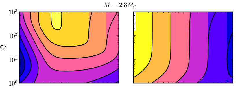
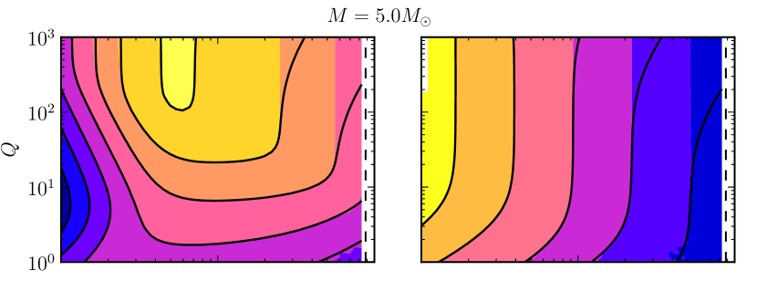
Figure 1: Comparison between simulations (shaded bands, color online) and approximation I (black contours) for different total masses. Left plots show the trigger SNR, right ones the delay. The dashed line is the ISCO frequency. As can be seen, this approximation fails for large $f_{0}$, $Q$ or $M$.

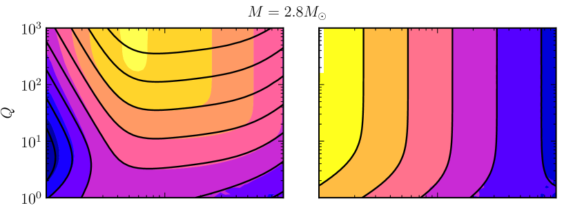
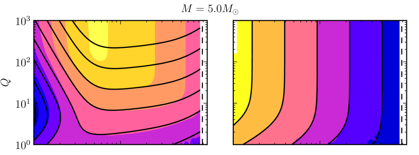
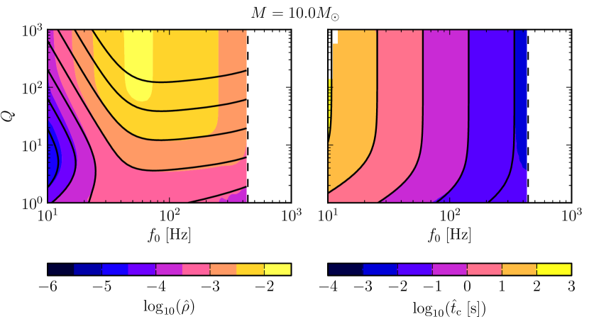
Figure 2: Comparison between simulations (shaded bands, color online) and approximation II (black contours) for different total masses. Left plots show the trigger SNR, right ones the delay. The dashed line is the ISCO frequency. The SNR predicted by approximation II is not correct for $Q\gg 1$, as expected. Remarkably however, the predicted trigger time is good for most of the explored parameter space.

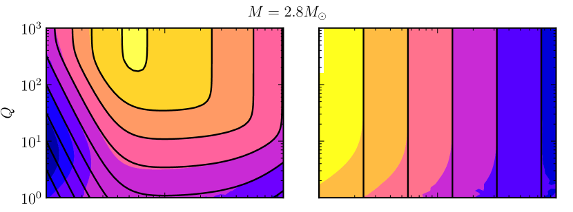
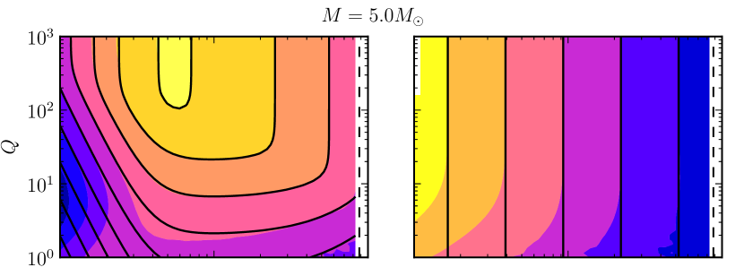
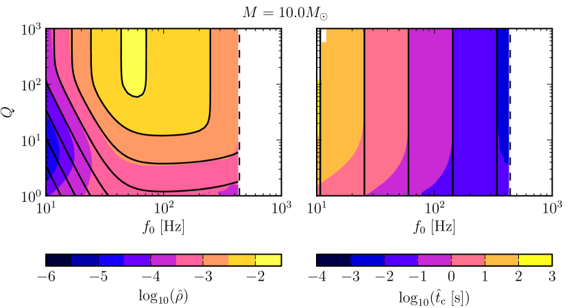
Figure 3: Comparison between simulations (shaded bands, color online) and approximation III (black contours) for different total masses. Left plots show the trigger SNR, right ones the delay. The dashed line is the ISCO frequency. As expected, approximation III does not work for small $Q$.

Approximation I works well for both $\hat{\rho}$ and $\hat{t}_{\rm c}$, but it degrades for large values of $f_{0}$, $Q$ or mass. In particular, we find that surfaces of constant accuracy roughly match those of constant $f^{2}_{0}QM$; the 5% accuracy for SNR, at least in the explored parameter range, is at $f^{2}_{0}QM/M_{\odot}\approx 5\times 10^{7}$ s^-2. This is likely not a major problem, as we expect most glitches to last at most tens of cycles and affect mostly low frequencies. Moreover, at high frequency or mass the time delay is small and thus the problem we are considering is less important. Also note that neglecting the second exponential of (6) produces no noticeable effects even for $Q\approx 1$.

Approximation II produces excellent estimates of the time delay across all the explored parameter space, but wrong estimates of SNR for large $Q$, as can be expected. In fact, as $Q$ increases, the sine-Gaussian peak in the frequency domain shrinks and at some point the integral is no longer dominated by the region around $f_{\rm s}$. Since we are interested in the low-$Q$ region, despite this problem this is still a useful approximation, although not significantly simpler than I.

As expected, approximation III works very well in the high mass, high $Q$ region where the other two approximations do not give such good results. Moreover it is analytically simpler. But for a large region of the parameter space where $Q$ is small, this approximation fails and so is not so useful for a large part of the parameter space of interest. This is because the width of the Gaussian in the frequency domain becomes comparable or larger than the width of the other terms in the integrand and the approximation is not valid. However, in this part of the parameter space we can simply revert to approximations I and II.

Although our calculations are based on the Newtonian chirp, search pipelines use inspiral waveforms with higher post-Newtonian order [6]. Thus we also check the accuracy of the approximations against simulations using a 3.5PN inspiral filter. We find that the accuracy degrades but is still within a few percent both for $\hat{\rho}$ and $\hat{t}_{\rm c}$ and it retains a similar dependency on $f_{0}$, $Q$ and $M$. An example for a $5M_{\odot}$ equal-mass binary is shown in figure 4. Since our approximations are based simply on power-series approximations of the inspiral phase, they can in principle accommodate high post-Newtonian order waveforms, at the price of more complicated expressions for $\rho(t_{\rm c})$.

Figure 4: Comparison between a simulation using a 3.5PN equal-mass inspiral waveform (shaded bands, color online) and approximation I (black contours) for a total mass of $5M_{\odot}$. The left plot is the trigger SNR, the right one is the trigger delay. The dashed line is the ISCO frequency.

In a search pipeline, the parameter space of the binary is covered by a template bank. A true inspiral signal produces triggers only for templates whose parameters are close enough to the true values, depending on the ambiguity function of the waveform. However, a strong glitch generally excites a significant fraction of the whole bank, producing a cluster of triggers with different SNRs and times. An example of this phenomenon is shown in figure 5, where we plot the distribution of triggers in $(\hat{t}_{\rm c},\hat{\rho})$ corresponding to a sine-Gaussian glitch affecting a simplified template bank with uniform distribution in total mass. The dependency of SNR and time delay on the template mass determines the shape of the cluster. Low-mass templates produce the triggers with the largest delay and smallest SNR. The last triggers can be delayed by several minutes, which is much longer than the duration of the glitch (typically seconds or fractions of a second).

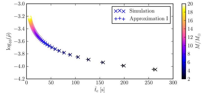
Figure 5: Cluster of triggers generated by a template bank responding to a sine-Gaussian glitch with $t_{0}=0$, $f_{0}=20$ Hz and $Q=20$. The bank consists of 50 3.5PN, equal-mass waveforms with $M$ uniformly spaced in $[2M_{\odot},20M_{\odot}]$. The cluster extends well after the duration of the glitch, with the lowest mass templates still producing triggers minutes after the glitch.

Again we stress that, since we considered the response of the matched filter to a noiseless sine-Gaussian glitch, the predicted coalescence time and SNR represent expectation values. Triggers produced by glitches in real data will have parameters distributed around our prediction. In particular we expect that, in the limit of high SNR, such distributions will tend to Gaussians centered on our prediction.

5 Conclusion

The length of low-mass inspiral filters represents a potential problem for future inspiral searches and in particular for low-latency BNS pipelines such as MBTA [16] and LLOID [17]. In fact, as evident from this study, short glitches with sine-Gaussian-like waveforms can produce low-mass triggers well after their occurrence time. Combined with the fact that a glitch can have significant overlap with a large fraction of the template bank, this implies that a single glitch can produce a cluster of many spurious triggers spanning a time interval of several minutes. Although we found that the trigger SNR effectively decreases with increasing delay, glitches can be very strong and still produce triggers with a large delay and SNR above the detection threshold. Consistency tests such as Allen’s $\chi^{2}$ [10], bank $\chi^{2}$ and auto $\chi^{2}$ [11] are most effective for long waveforms and would likely rule out a large fraction of such spurious triggers. A detailed investigation of the response and effectiveness of these tests with respect to sine-Gaussian waveforms is a necessary followup of this work and could provide hints at how to optimally tune the parameters of such tests for this particular glitch model.

Unfortunately however, the efficiency of consistency tests also decreases with decreasing SNR. Triggers with large delay and SNR just above the detection threshold will therefore still be problematic and the usual veto procedures based on auxiliary channels will be required. For past searches, such procedures consisted in identifying glitches in one or more auxiliary channels and excluding inspiral triggers within an appropriate coincidence window. While this method is applicable in the case of short inspiral filters, though, its naive application to future low-mass searches would remove all triggers within hundreds or thousands of seconds around each glitch, significantly reducing the live time of the experiment.

We presented three approximations which allow one to predict the SNR and time of spurious triggers generated by an inspiral matched filter responding to sine-Gaussian glitches. Such formulae effectively map the parameters of the glitch and the chirp mass of the template to the SNR and time of the resulting spurious trigger. In other words, they represent the first step in understanding false inspiral triggers produced by isolated, sine-Gaussian glitches. We compared them to numerical simulations and investigated their validity in the region of $(f_{0},Q,\mathcal{M})$ parameter space relevant for advanced detectors. Together they complement each other, providing full coverage of the explored region.

The formulae can be used for vetoing spurious low-mass triggers in the following way. Assuming we have knowledge of a non-astrophysical, sine-Gaussian-like excitation in the strain data—either from a burst search pipeline such as Omega [18], or by identifying excitations in auxiliary channels with known couplings to the strain channel [19]—we can predict for each template the SNR and time of the resulting inspiral triggers. We can then scan the list of triggers produced by the inspiral search and look for the ones matching the predicted SNR and time, within a coincidence window accounting for the uncertainty in the prediction due, for instance, to the detector noise. Triggers found in coincidence with the prediction can then be associated with the glitch and selectively removed. Alternatively, if enough coincident triggers are found, the portion of strain data corrupted by the glitch can be removed—for instance by replacing it with Gaussian noise—and the inspiral search repeated. This would essentially remove the whole cluster of triggers produced by the glitch without sacrificing a segment of analysis time as long as the longest filter. The more precise definition, implementation and testing of this procedure constitute another natural followup of this paper.

References

References

- [1] Harry G M et al. 2010 Advanced LIGO: the next generation of gravitational wave detectors Class. Quant. Grav. 27 084006
- [2] Acernese F et al. 2009 Advanced Virgo Baseline Design Virgo Technical Report VIR-0027A-09
- [3] Abadie J et al. 2010 Predictions for the Rates of Compact Binary Coalescences Observable by Ground-based Gravitational-wave Detectors Class. Quant. Grav. 27 173001
- [4] Blanchet L 2006 Gravitational Radiation from Post-Newtonian Sources and Inspiralling Compact Binaries Living Rev. Rel. 9
- [5] Babak S et al. 2013 Searching for gravitational waves from binary coalescence Phys. Rev. D 87 024033
- [6] Allen B et al. 2012 FINDCHIRP: an algorithm for detection of gravitational waves from inspiraling compact binaries Phys. Rev. D 85 122006
- [7] Blackburn L et al. 2008 The LSC Glitch Group: Monitoring Noise Transients during the fifth LIGO Science Run Class. Quant. Grav. 25 184004
- [8] Aasi J et al. 2012 The characterization of Virgo data and its impact on gravitational-wave searches Class. Quant. Grav. 29 155002
- [9] Slutsky J et al. 2010 Methods for reducing false alarms in searches for compact binary coalescences in LIGO data Class. Quant. Grav. 27 165023
- [10] Allen B 2005 A chi-squared time-frequency discriminator for gravitational wave detection Phys. Rev. D 71 062001
- [11] Hanna C 2008 Searching for gravitational waves from binary systems in non-stationary data PhD thesis, Louisiana State University
- [12] Sathyaprakash B S and Dhurandhar S V 1991 Choice of filters for the detection of gravitational waves from coalescing binaries Phys. Rev. D 44 3819
- [13] Peters P C and Mathews J 1963 Gravitational Radiation from Point Masses in a Keplerian Orbit Phys. Rev. 131 435–-440
- [14] Sengupta A S et al. 2003 A faster implementation of the hierarchical search algorithm for detection of gravitational waves from inspiraling compact binaries Phys. Rev. D 67 082004
- [15] https://www.lsc-group.phys.uwm.edu/daswg/projects/lalsuite.html
- [16] Beauville F et al. 2008 Detailed comparison of LIGO and Virgo Inspiral Pipelines in Preparation for a Joint Search Class. Quant. Grav. 25 045001
- [17] Cannon K et al. 2012 Toward Early-warning Detection of Gravitational Waves from Compact Binary Coalescence ApJ 748 136
- [18] Chatterji, S K 2005 The search for gravitational wave bursts in data from the second LIGO science run PhD thesis, MIT Dept. of Physics
- [19] Ajith P, Hewitson M, Smith J R, Grote H and Hild S 2007 Physical instrumental vetoes for gravitational-wave burst triggers Phys. Rev. D 76 042004