MESA and NuGrid simulations of classical novae: CO and ONe nova nucleosynthesis

Abstract

Classical novae are the result of thermonuclear flashes of hydrogen accreted by CO or ONe white dwarfs, leading eventually to the dynamic ejection of the surface layers. These are observationally known to be enriched in heavy elements, such as C, O and Ne that must originate in layers below the H-flash convection zone. Building on our previous work, we now present stellar evolution simulations of ONe novae and provide a comprehensive comparison of our models with published ones. Some of our models include exponential convective boundary mixing to account for the observed enrichment of the nova ejecta even when accreted material has a solar abundance distribution. Our models produce maximum temperature evolution profiles and nucleosynthesis yields in good agreement with models that generate enriched ejecta by assuming that the accreted material was pre-mixed. We confirm for ONe novae the result we reported previously, i.e. we found that ³He could be produced in situ in solar-composition envelopes accreted with slow rates ($\dot{M}<10^{-10}\,M_{\odot}/\mbox{yr}$) by cold ($T_{\rm WD}<10^{7}$ K) CO WDs, and that convection was triggered by ³He burning before the nova outburst in that case. In addition, we now find that the interplay between the ³He production and destruction in the solar-composition envelope accreted with an intermediate rate, e.g. $\dot{M}=10^{-10}\,M_{\odot}/\mbox{yr}$, by the $1.15\,M_{\odot}$ ONe WD with a relatively high initial central temperature, e.g. $T_{\rm WD}=15\times 10^{6}$ K, leads to the formation of a thick radiative buffer zone that separates the bottom of the convective envelope from the WD surface. We present detailed nucleosynthesis calculations based on the post-processing technique, and demonstrate in which way much simpler single-zone $T$ and $\rho$ trajectories extracted from the multi-zone stellar evolution simulations can be used, in lieu of full multi-zone simulations, to analyse the sensitivity of nova abundance predictions on nuclear reaction rate uncertainties. Trajectories for both CO and ONe nova models for different central temperatures and accretion rates are provided. We compare our nova simulations with observations of novae and pre-solar grains believed to originate in novae.

1 Introduction

Classical nova explosions are a consequence of thermonuclear runaways (TNR) occurring in accreted H-rich shells on the white dwarf (WD) components of close binary systems. The accumulation of H-rich shells on the surfaces of the WD components of these systems continues until a critical pressure $\sim 10^{19}\mathrm{dyne}/\mathrm{cm}^{2}$ is achieved at the base of the accreted envelope and runaway ensues. An increase in the shell burning luminosity then follows (at a rate that reflects/defines the speed class of the nova) to a value that approaches (and for fast novae can exceed) the Eddington limit. Following a period of burning at approximately constant bolometric luminosity, dictated by the core-mass-luminosity relation of Paczyński (1970), the nova ultimately returns to its pre-outburst state. The occurrence of mass loss from novae through outburst yields an ejected envelope, the composition of which reflects both the consequences of the thermonuclear burning epoch and the occurrence of dredge-up of matter from the underlying WD into the H-rich envelope.

Our understanding of the nova phenomenon has increased substantially over the past several decades as a consequence of significant progress in theoretical modeling of their outbursts, of significantly improved observational determinations of the characteristics of novae throughout outburst, and of the acquisition of greatly improved abundance data concerning both the compositions of the accreted shells and, particularly, the nebular ejecta of diverse nova systems (Truran, 1982; Starrfield, 1989; Shara, 1989; Gehrz et al., 1998; Downen et al., 2013, and references therein). Multidimensional hydrodynamic simulations of classical novae are also available (Glasner et al. 1997, 2005, 2012; Casanova et al. 2010, 2011; Kercek et al. 1998).

A critical feature of novae seen in outburst is the fact that diverse nova systems have been found to be characterized by significant enrichments of many of the elements, such as C, N, O, Ne, Na, Mg, or Al, relative to H, with respect to solar abundances. It is generally expected that, for the temperature/density conditions that characterize the burning shells of most novae (with peak shell temperatures typically less than $4\times 10^{8}\mathrm{K}$), significant breakout of the CNO H-burning sequences cannot occur (Wiescher et al., 1986; Yaron et al., 2005). It then follows that the elevated total abundance of heavy elements between He and Ca, as compared to their combined solar mass fraction of less than 2%, arise from dredge-up from the underlying cores, followed by their reshuffling in the H-shell burning. C, N, and O are enriched by dredge-up from CO WDs, while the observed abundance enrichments of C, O, and Ne arise from the outward mixing or dredge-up of matter from an underlying ONe WD.

ONe novae are of particular interest for nucleosynthesis because they develop the highest temperatures during the nova outburst. They also represent an unexpectedly large fraction of observed novae. Tables of abundances in nova ejecta were published in both the papers on nova composition by Truran & Livio (1986), Livio & Truran (1994) and Downen et al. (2013) and the review paper by Gehrz et al. (1998). In the more extended compilation by Gehrz et al. (1998) out of the 20 novae ten are clearly CO novae (mass fraction ratios of $\mathrm{Ne}/\mathrm{Ne}_{\odot}<8$), while seven (three) are clearly (possibly) ONe novae ($\mathrm{Ne}/\mathrm{Ne}_{\odot}>10-15$). However, the fraction of ONe white dwarfs in the Galaxy is expected to be much smaller, based on models of stellar evolution. Carbon ignition happens only for (super-)Asymptotic Giant Branch (AGB) stars with core masses greater than $\sim 1.05M_{\odot}$, and ONe WDs can only form in stars with initial masses in the corresponding narrow range of $\sim 7-10M_{\odot}$ (depending on metallicity and mixing assumptions during H- and He-core burning phases) that features C ignition but avoids core-collapse supernova. Although the details of this simulation prediction depend sensitively on the ${}^{12}\mathrm{C}+{{}^{12}\mathrm{C}}$ reaction rate (Chen et al., 2013) as well as on the physics details of the C-flame for off-center C ignition (Denissenkov et al., 2013), present best estimates based on a Salpeter initial mass function predict that the ratio of CO to ONe WDs is approximately thirty (Livio & Truran, 1994; Gil-Pons et al., 2003).

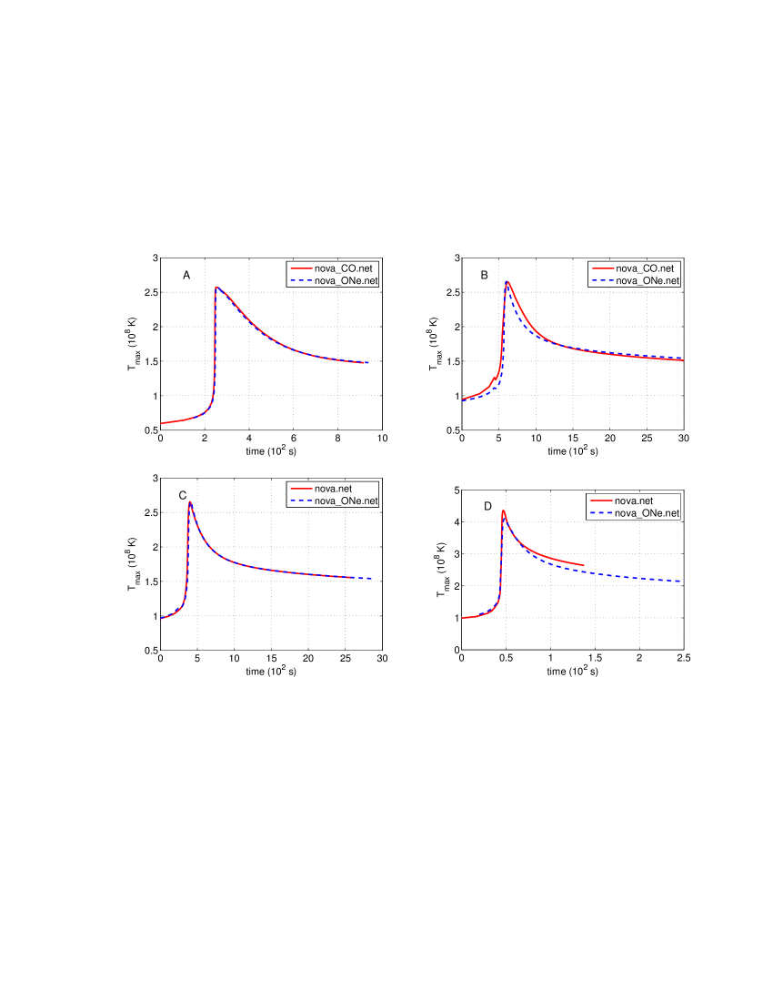
Figure 1: Comparison of $T_{\rm max}$-trajectories extracted from our MESA CO and ONe nova simulations that were carried out using different nuclear networks: nova_CO.net that includes only 33 isotopes from H to ²⁶Mg coupled by 65 reactions, nova_ONe.net that extends the first network to 48 isotopes from H to ³⁰Si coupled by 120 reactions, and the largest network nova.net with 77 isotopes from H to ⁴⁰Ca and 442 reactions. Panel A: our $1.15\,M_{\odot}$ CO nova simulations for $T_{\rm WD}=10$ MK ($\log_{10}L_{\rm WD}/L_{\odot}=-2.69$; for the correspondence between WD’s initial central temperature and luminosity, $T_{\rm WD}$ and $L_{\rm WD}$, see Table 1) and $\dot{M}=10^{-11}\,M_{\odot}/\mbox{yr}$. Panels B and C: our simulations of $1.15\,M_{\odot}$ and $1.3\,M_{\odot}$ ONe novae, respectively, for the same values of $T_{\mathrm{WD}}=12$ MK and $\dot{M}=2\times 10^{-10}\,M_{\odot}/\mbox{yr}$. Panel D: the most extreme case of ONe nova with $T_{\mathrm{WD}}=7$ MK and $\dot{M}=10^{-11}\,M_{\odot}/\mbox{yr}$. All these simulations assume that the WD accretes a mixture of equal amounts of its core and solar-composition materials.

Denissenkov et al. (2013, hereafter Paper I) presented 1D simulations of nova outbursts occurring on CO WDs based on the MESA stellar evolution code (Paxton et al., 2011, 2013). In the present paper, we complement those results with MESA models of ONe nova outbursts. In addition, the multi-zone post-processing code MPPNP, which is a part of the NuGrid research framework (Herwig et al. 2008), is used here for computations of detailed nucleosynthesis in CO and ONe novae. The MESA nova models provide MPPNP with necessary stellar structure and mixing parameter profiles. The NuGrid tools also include the single-zone code SPPN that enables post-processing nucleosynthesis computations along a $(T,\rho)$ trajectory, for example at one Lagrangian coordinate (a mass zone) inside 1D stellar models, or along the position of the maximum temperature. We have run SPPN for trajectories tracing the evolution of the maximum temperature in the nova envelope (usually at the core-envelope interface) and its corresponding density. We show that, because of the strong dependence of thermonuclear reaction rates on $T$, nucleosynthesis yields obtained with the SPPN code for the $T_{\rm max}$-trajectories are in qualitative agreement with the complete yields provided by the MPPNP code. The SPPN code runs much faster than MPPNP, therefore it can be used for a comprehensive numerical analysis of parameter space, for example, when the relevant reaction rates are varied within their experimentally constrained limits.

We have prepared Linux shell scripts, template MESA inlist files, and a large number of initial WD models aiming to combine MESA and NuGrid into an easy-to-use Nova Framework. This new research tool can model nova outbursts and nucleosynthesis occurring on CO and ONe WDs using up-to-date input physics and a specified nuclear network for a relatively large number (up to a few thousands) of mass zones covering both the WD and its accreted envelope. Nova simulation results can be analyzed using animations and a variety of plots produced with NuGrid’s Python visualization scripts. One of the main goals of this paper is to demonstrate Nova Framework’s capabilities.

The simulation tools of MESA and NuGrid are described in Section 2. The MESA models of nova outbursts occurring on CO and ONe WDs are discussed in Section 3. Results of the post-processing nucleosynthesis computations for CO and ONe novae obtained with the NuGrid codes MPPNP and SPPN are presented in Section 4. In Section 5, we describe the effects of ³He in situ production and burning on triggering convection in the accreted solar-composition envelopes of ONe novae. A comparison of our results of the nova nucleosynthesis simulations with available data on nova-related element and isotope abundances from spectroscopic and presolar grain composition analyses is made in Section 6. Finally, our main conclusions are drawn in Section 7.

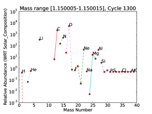
Figure 2: Relative (with respect to solar) abundances (mass fractions) of stable isotopes calculated with the NuGrid multi-zone post-processing nucleosynthesis code MPPNP, averaged over the indicated mass range (in $M_{\odot}$) in the expanding envelope, in a final model (its number, called “Cycle” in MPPNP, is 1300) of our $1.15\,M_{\odot}$ CO nova simulations with $T_{\rm WD}=15$ MK and $\dot{M}=2\times 10^{-10}\,M_{\odot}/\mbox{yr}$ (compare with Fig. 1 of José & Hernanz (1998) and Fig. 5 in Paper I). Isotopes of the same elements are connected by lines of different colors and styles to better distinguish them visually.

2 Simulation Tools

2.1 Stellar Evolution Calculations – MESA

MESA is a collection of Fortran-95 Modules for Experiments in Stellar Astrophysics. Its star module can be used for 1D stellar evolution simulations of almost any kind (numerous examples are provided by Paxton et al. (2011, 2013) and on the MESA users’ website mesastar.org). Other MESA modules provide star with state-of-the-art numerical algorithms, e.g. for adaptive mesh refinement and timestep control, atmospheric boundary conditions, and modern input physics (opacities, equation of state (EOS), nuclear reaction rates, etc.)

For our MESA simulations of ONe nova outbursts, we use the same EOS and opacity tables that were used to model the CO novae in Paper I. The only important difference is our adoption of longer lists of isotopes and reactions for the ONe nova models. The adopted nuclear network has to be as large as necessary in order to account for the energy generation during a nova TNR, yet as small as possible in order to make computations not too time consuming. We have started our MESA nova simulations with the largest network nova.net that includes 77 isotopes from H to ⁴⁰Ca coupled by 442 reactions. This network has a list of isotopes almost identical to that selected by Weiss & Truran (1990), Politano et al. (1995), and Starrfield et al. (2009). We have gradually reduced the numbers of isotopes and reactions checking that this does not lead to significant changes in the time variations of the maximum temperatures and their corresponding densities at the bottoms of accreted envelopes during nova outbursts that we call “$T_{\rm max}$-trajectories”. As a result, acceptable compromises satisfying the above qualitative criteria have been found empirically. A list of 33 isotopes coupled by 65 reactions, including those of the pp chains (the pep reaction, whose importance was emphasized by Starrfield et al. (2009), has also been added), CNO and NeNa cycles, was selected for our CO nova models in Paper I. We will call this nuclear network nova_CO.net. A similar selection procedure for the ONe nova models has resulted in a necessity to adopt an extended nuclear network nova_ONe.net that includes 48 isotopes from H to ³⁰Si coupled by 120 reactions. The $T_{\rm max}$-trajectories extracted from our CO and ONe nova simulations performed for different sets of nova parameters using the three nuclear networks are compared in Fig. 1. From these plots, it is seen that the nova_CO.net and nova_ONe.net nuclear networks provide an acceptable accuracy for the simulations of CO and ONe nova outbursts, respectively. Indeed, the upgrade from the first to the second network does not noticeably change the $T_{\mathrm{max}}$-trajectories in our simulations of the CO nova outbursts, even when a cold CO WD accretes at a very low rate, which leads to a stronger TNR (panel A). Likewise, in all the ONe cases (e.g., panel C), except the most extreme one shown in panel D, replacing nova_ONe.net with nova.net does not change much their corresponding $T_{\mathrm{max}}$-trajectories.

Depending on the values of initial parameters, nuclear network and assumptions about mixing, an individual MESA nova simulation on a modern personal computer can take from a few minutes to a few hours.

By default, MESA uses reaction rates from Caughlan & Fowler (1988) and Angulo et al. (1999), with preference given to the second source (NACRE). It includes updates to the NACRE rates for ¹⁴N(p,$\gamma)^{15}$O (Imbriani et al. 2005), the triple-$\alpha$ reaction (Fynbo et al. 2005), ¹⁴N$(\alpha,\gamma)^{18}$F (Görres et al. 2000), and ¹²C$(\alpha,\gamma)^{16}$O (Kunz et al. 2002). Although the main nuclear path for a classical nova is driven by p-capture reactions and $\beta$-decays, the $\alpha$-reactions are important for establishing the chemical composition of its underlying WD (MESA has also been used to prepare WD models for our CO and ONe nova simulations, see Section 3.2).

2.2 Nucleosynthesis Calculations – NuGrid

The nucleosynthesis calculations were performed with the post-processing code PPN (either for single-zone or multi-zone post-processing, Herwig et al., 2008; Pignatari & Herwig, 2012), where the input data of stellar structure (here from MESA models) are processed using a dynamically updated list of nuclear species and reaction rates. The network can include more than 5000 species, between H and Bi, and more than 50000 nuclear reactions. The self-adjusting dynamical network has at any point in the simulation (and in each layer for multi-zone simulations) a suitable size, based on the strength of nucleosynthesis fluxes, $\delta Y_{\rm i}/\delta t_{\rm j}$, that show the variation rates of the abundances $Y_{\rm i}=X_{\rm i}/A_{\rm i}$ due to the reactions $j$. Rates are taken from different data sources: the European NACRE compilation (Angulo et al., 1999) and Iliadis et al. (2001), or more recent, if available (e.g., Fynbo et al., 2005; Kunz et al., 2002; Imbriani et al., 2005), and the JINA Reaclib v1.1 library (Cyburt et al., 2010). For neutron capture rates by stable nuclides and a selection of relevant unstable isotopes, NuGrid uses the Kadonis compilation (http://www.kadonis.org), although neutron captures are not important for the present work. For weak reaction rates, we choose between Fuller (1985), Oda et al. (1994), Langanke & Martínez-Pinedo (2000) and Goriely (1999), according to the mass region.

For the complete post-processing of the full MESA nova models, we use the multi-zone parallel frame of PPN (MPPNP). For single $(T,\rho)$ trajectories, the post-processing is done with the single-zone version SPPN. Both variants use the same nuclear physics library and the same package to solve the nucleosynthesis equations.

3 MESA Models of Nova Outbursts

In Paper I, we presented MESA models of CO nova outbursts for a number of initial CO WD masses and temperatures (luminosities). For completeness, we include some of the CO nova outburst models here as well, and then present the new ONe nova models. The nucleosynthesis in both model families is then analysed using the NuGrid tools.

3.1 CO Novae

A few CO nova models are included in the present discussion as a link to Paper I and also as an illustration of application of the NuGrid MPPNP code for post-processing of CO nova models. All the results relevant to the CO nova models are presented in Figs. 1A, 2, 3, and at the beginning of Table 1. Fig. 1A compares two $T_{\rm max}$-trajectories extracted from our MESA simulations of nova outbursts occurring on a CO WD with the same mass, $M_{\rm WD}=1.15\,M_{\odot}$, and initial central temperature, $T_{\rm WD}=10$ MK ($\log_{10}L_{\rm WD}/L_{\odot}=-2.69$; for the correspondence between WD’s initial central temperature and luminosity, $T_{\rm WD}$ and $L_{\rm WD}$, see Table 1), and for the same accretion rate, $\dot{M}=10^{-11}\,M_{\odot}/\mbox{yr}$. The only difference between the models is that the one has been computed using the small nuclear network nova_CO.net that includes 33 isotopes from H to ²⁶Mg coupled by 65 reactions, while the other with the extended network of 48 isotopes and 120 reactions, nova_ONe.net. The good agreement between the two trajectories, even for a relatively low $T_{\rm WD}$ and slow accretion rate that lead to a stronger outburst, confirms our choice of nova_CO.net as a sufficient nuclear network for the MESA CO nova models in Paper I. Fig. 2 shows the results of the post-processing nucleosynthesis simulations carried out for one of the CO nova models considered in Paper I. Our final abundances of the stable isotopes divided by their corresponding solar abundances change with the increasing mass number in a fashion closely resembling that seen in Fig. 1 of José & Hernanz (1998) for a CO nova model with similar parameters as well as that produced by the MESA code alone (see Fig. 5 in Paper I). However, when our nova yields are compared with those from the literature for individual isotopes, the differences can reach an order of magnitude for some isotopes, or even a larger factor for a few other isotopes. A similar conclusion can also be made when one compares on an isotope by isotope basis the nova yields published by José & Hernanz (1998) and Starrfield et al. (2009). This is probably caused by differences in many ingredients, such as initial abundances, reaction rates, computer code details etc., that are used to model nova outbursts.

Table 1: Parameters of Computed Nova Models

WD	$M_{\rm WD}[\,{\rm M}_{\odot}]$	$T_{\rm WD}[10^{6}\,\mathrm{K}]$	$\lg L_{WD}[\mathrm{L_{\odot}}]$	$M_{\mathrm{acc}}[10^{-5}\,{\rm M}_{\odot}]$	$\lg L_{\mathrm{H}}[\mathrm{L_{\odot}}]$	$T_{\mathrm{max}}[10^{6}\,\mathrm{K}]$	Nucl. Network	Init. Comp.
CO	1.0	12	-2.55	5.2	10.88	200	nova_CO	MESA
CO	1.0	20	-1.99	2.1	9.59	163	nova_CO	MESA
COa,b	1.15	10	-2.69	4.0	11.84	257	nova_CO, nova_ONe	MESA
CO	1.15	12	-2.50	2.8	11.27	236	nova_CO	MESA
COc	1.15	12	-2.50	9.7	11.28	243	nova_CO	MESA
CO	1.15	15	-2.25	1.6	10.45	208	nova_CO	MESA
CO	1.15	20	-1.94	0.94	9.67	185	nova_CO	MESA
ONeb	1.15	12	-2.54	4.0	10.24	262	nova_CO, nova_ONe	MESA
ONeb	1.15	12	-2.54	4.0	10.14	263	nova_ONe, nova	MESA
ONec	1.15	12	-2.54	15.0	9.89	245	nova_ONe	MESA
ONe	1.15	20	-2.03	3.0	9.88	245	nova_ONe	MESA
ONe	1.15	20	-2.03	2.0	9.46	219	nova_ONe	Barcelona
ONea	1.3	7	-3.05	3.0	10.82	408	nova_ONe, nova	MESA
ONe	1.3	12	-2.52	1.7	10.23	357	nova_ONe	Politano
ONe	1.3	12	-2.52	1.5	10.60	344	nova_ONe	Barcelona
ONe	1.3	15	-2.29	0.95	9.90	313	nova_ONe	Barcelona
ONe	1.3	20	-1.98	1.0	9.86	318	nova_ONe, nova	MESA
ONe	1.3	20	-1.98	0.52	9.26	267	nova_ONe	Barcelona
ONe	1.3	20	-1.98	0.53	9.29	266	nova (NACRE)	Barcelona
ONe	1.3	20	-1.98	0.52	9.37	265	nova (JINA)	Barcelona

^aThis model uses the accretion rate $\dot{M}=10^{-11}\,M_{\odot}/\mbox{yr}$, while all other $\dot{M}=2\times 10^{-10}\,M_{\odot}/\mbox{yr}$.

^bFor simulations done for two different nuclear networks, e.g. nova_ONe.net and nova.net, only the results for the first case are shown (for the network highlighted with a bold font).

^cThis simulation includes CBM with $f=0.004$, like in Paper I, while all other assume that the WD accretes a mixture of equal amounts of its core and solar-composition materials. For this case, $M_{\mathrm{acc}}$ gives the mass of H-rich envelope that includes WD’s outer layers penetrated by the CBM.

3.2 ONe Novae

According to Gil-Pons et al. (2003), the frequency of occurrence of galactic ONe novae in close binary systems is expected to be 30% to 40%, depending on model assumptions. Without convective overshooting of H-core burning, the range of initial masses of the stars that end their evolution as ONe WDs with the masses between $1.1M_{\odot}$ and $1.33M_{\odot}$ is estimated by the same authors to be between $9.3M_{\odot}$ and $12M_{\odot}$.

Two ONe WD models with the masses $M_{\rm WD}=1.15\,M_{\odot}$ and $1.3\,M_{\odot}$ have been prepared by us with MESA for a range of initial central temperatures and luminosities using the same “stellar engineering” procedure with which we created the CO WD models in Paper I (Table 1, note that the $L_{\mathrm{WD}}(T_{\mathrm{WD}})$ relation is almost universal for the CO and ONe WDs for $M_{\mathrm{WD}}\geq 1.0M_{\odot}$). Likewise, we have artificially removed the He- and C-rich buffer zones from the surfaces of ONe WD models and used the naked ONe WDs with thin ($\sim$ $10^{-7}\,M_{\odot}$) H-rich envelopes as the initial models for ONe nova simulations. The ONe WD models were created using the same isotopes as in nova.net, while the reaction list was extended to take into account He and C burning.

We have not included any prescription for mass loss in the MESA ONe nova simulations, yet we have followed the hydrodynamic expansion of the nova envelopes until their surface radii exceeded a few solar radii. This should guarantee that the expanding envelope has crossed the WD’s Roche-lobe radius for a typical binary system hosting a classical nova (e.g., Paper I). The ONe nova evolutionary tracks are not much different from our CO nova tracks discussed in Paper I (e.g., Fig. 3). A more detailed discussion of nova model light curves is beyond the scope of the present study, which is mainly focused on the nova outburst phase and nucleosynthesis.

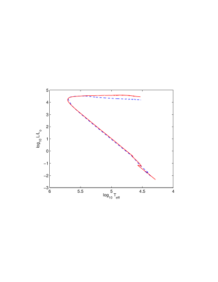
Figure 3: Evolutionary tracks for pre-mixed CO (solid red curve) and ONe (dashed blue curve) nova models computed with the MESA code for the same initial parameters: $M_{\mathrm{WD}}=1.15M_{\odot}$, $T_{\mathrm{WD}}=12$ MK, and $\dot{M}=2\times 10^{-10}M_{\odot}/\mathrm{yr}$.

Like for the CO nova simulations in Paper I, here we consider three types of ONe nova models. A few models are of the first type: they neglect boundary mixing (adopting a strict Schwarzschild condition to determine the convective boundary) and assume that the WD accretes solar-composition material (e.g., the models with the in situ ³He production that are discussed in Section 5). For solar composition we use the elemental abundances of Grevesse & Noels (1993) with the isotopic abundance ratios from Lodders (2003). These models do neither show the fast rise time nor the enhancements in heavy elements observed for novae.

A realistic nova model should assume that the accreted material has solar composition (for solar metallicity) and that it is mixed with the WD’s material before or during its thermonuclear runaway. Recent two- and three-dimensional nuclear-hydrodynamic simulations of a nova outburst have shown that a possible mechanism of this mixing are the hydrodynamic instabilities and shear-flow turbulence induced by steep horizontal velocity gradients at the bottom of the convection zone triggered by the runaway (Casanova et al., 2010, 2011). These hydrodynamic processes associated with the convective boundary lead to convective boundary mixing (CBM) at the base of the accreted envelope into the outer layers of the WD. As a result, CO-rich (or ONe-rich) material is dredged up during the runaway. In our 1D MESA simulations of nova outbursts, we use a simple CBM model that treats the time-dependent mixing as a diffusion process. The model approximates the rate of mixing by an exponentially decreasing function of a distance from the formal convective boundary (Freytag et al., 1996; Herwig et al., 1997)

$$D_{\rm CBM}=D_{0}\exp\left(-\frac{2|r-r_{0}|}{fH_{P}}\right),$$ (1)

where $H_{P}$ is the pressure scale height, and $D_{0}$ is a diffusion coefficient, calculated using a mixing-length theory, that describes convective mixing at the radius $r_{0}$ close to the boundary. In this model $f$ is a free parameter, for which we use the same value $f=f_{\mathrm{nova}}=0.004$ that we used in our CO nova simulations in Paper I, where it led to the heavy-element enrichment of nova envelope comparable to those found in both multi-dimensional hydrodynamic simulations and in the spectroscopic measurements of heavy-element abundances in nova ejecta. We have varied $f_{\mathrm{nova}}$ to estimate the sensitivity of our results to its value. It turns out that very similar nova nucleosynthesis yields are obtained when we increase $f_{\mathrm{nova}}$ from 0.004 to 0.006, while outside of this range the CBM dredges up either too little or too much WD’s material to match the observational data. The second type of our nova models takes into account the CBM (e.g., the CBM models in Figs. 12 and 13). These models do match observed rise times and abundances.

Finally, most of our models (Table 1) are of type three in which CBM is neglected, like in the first-type models. However, the effect of CBM is artificially obtained by assuming that the WD accretes a mixture in which solar-composition material has already been blended with an equal amount of WD material.

Such pre-mixed models are commonly adopted in 1D nova simulations. The fraction of WD’s material in the mixture can vary from 25% up to 75% to match observed values (e.g., José & Hernanz 1998). To prepare the initial pre-mixed abundances, we have used the isotope abundances from the outermost layers of our naked ONe WD models. Our initial pre-mixed abundances for the $1.3M_{\odot}$ ONe nova model (of the third type) are compared with the 50% pre-mixed abundances that we call the Barcelona and Politano compositions in Fig. 4. The Barcelona data are taken from José et al. (1999, 2001). They contain material from a $1.35M_{\odot}$ ONe WD model. The Politano data are from Politano et al. (1995). They were derived from the C-burning nucleosynthesis calculations of Arnett & Truran (1969). Our initial abundances agree quite well with those from the Barcelona composition (the upper panel), especially for ¹⁶O, ²⁰Ne, and ²⁴Mg. As for the Politano composition (the lower panel of Fig. 4), it has similar to ours ¹⁶O and ²⁰Ne abundances, but much higher initial ²⁴Mg abundance (10% in mass fraction versus 3% in the Barcelona mixture). The last difference is important for ONe nova simulations because ²⁴Mg can compete with ¹²C in igniting the accreted H-rich material in the range of temperatures relevant to nova outbursts (Glasner et al. 2012). Our initial ¹²C abundance has a value intermediate between the 6% and 0.9% mass fractions in the Barcelona and Politano mixtures. The more recent massive AGB models (Ritossa et al., 1996), including ours, show that the ²⁴Mg abundance in ONe WDs is much smaller than the one assumed by Politano et al. (1995).

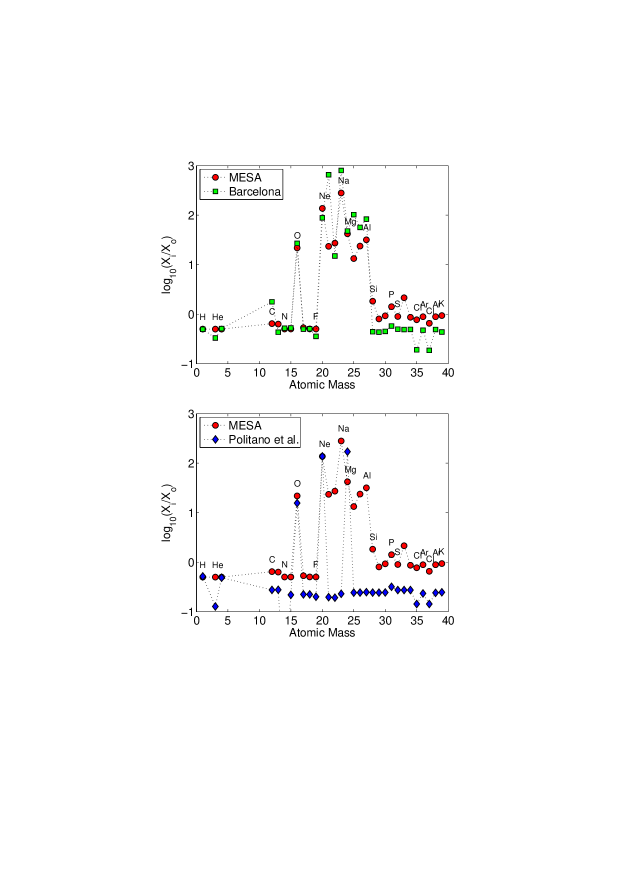
Figure 4: Initial abundances (solar-scaled mass fractions) of isotopes in the pre-mixed material accreted by our $1.3\,M_{\odot}$ ONe WD model (red circles) are compared with those used in similar nova models by the Barcelona group (José et al. 1999, 2001) (green squares in the upper panel) and by both Politano et al. (1995) and Starrfield et al. (2009) (blue diamonds in the lower panel). In all the cases, it is assumed that the WD accretes a mixture consisting of equal amounts of its core and solar-composition materials. Element symbols point to their corresponding most abundant isotopes in the Solar system (¹²C, ¹⁴N, ¹⁶O, ²⁰Ne, ²³Na, ²⁴Mg, ²⁷Al, etc.)

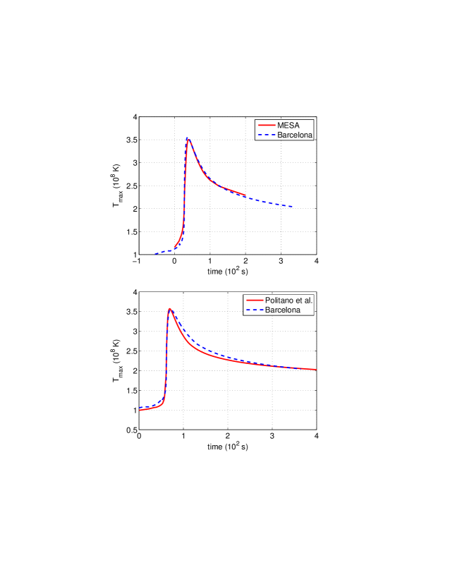
Figure 5: $T_{\mathrm{max}}$-trajectories from our simulations of $1.3\,M_{\odot}$ ONe novae carried out for the same values of $T_{\mathrm{WD}}=12$ MK and $\dot{M}=2\times 10^{-10}\,M_{\odot}/\mbox{yr}$, but for our considered three different initial compositions of the accreted material from Fig. 4.

In Fig. 1, we compare $T_{\mathrm{max}}$-trajectories extracted from our $1.15M_{\odot}$ (panel B) and $1.3M_{\odot}$ (panel C) ONe nova simulations for $T_{\mathrm{WD}}=12$ MK with pre-mixed material, in which isotope abundances from WD models of the corresponding masses were used, accreted with the rate $\dot{M}=2\times 10^{-10}M_{\odot}/\mathrm{yr}$. For either CO or ONe WD, the main properties of its nova outburst, such as total accreted ($M_{\mathrm{acc}}$) and ejected masses, peak temperature $T_{\mathrm{max}}$, maximum H-burning ($L_{\mathrm{H}}$) and total luminosities, envelope expansion velocity, and chemical composition of the ejecta, depend mainly on the following three parameters: the WD mass $M_{\rm WD}$, its central temperature $T_{\rm WD}$ (or luminosity $L_{\mathrm{WD}}$), and the accretion rate $\dot{M}$ (e.g., Prialnik & Kovetz 1995; Townsley & Bildsten 2004; José et al. 2007). The results also depend on a choice of nuclear network (lists of isotopes and reactions), initial abundances in the accreted material, reaction rates and other input physics (EOS, opacities), and computer code. For the present work, some of the initial and calculated nova model parameters are listed in Table 1. Here, we have only considered material (and mixtures thereof) of solar metallicity. In general, our pre-mixed ONe nova models computed with the Barcelona initial composition have systematically lower $M_{\mathrm{acc}}$ and $T_{\mathrm{max}}$ values, as compared to their counterparts computed with both MESA and Politano compositions. This is probably caused by the higher initial abundance of ¹²C in the Barcelona mixture (the upper panel of Fig. 4) that turns on the nova ignition a bit earlier.

To categorize our nova simulations carried out for the different sets of initial parameters, we use $T_{\mathrm{max}}$-trajectories (e.g., Fig. 1). They have two characteristics that determine the resulting nova speed class and nucleosynthesis: a peak value of the $T_{\mathrm{max}}$ curve and its width near the peak, the latter being proportional to a timescale of nova outburst. We have already used $T_{\mathrm{max}}$-trajectories to support our choice of nova_CO.net as a sufficient nuclear network for MESA CO nova simulations (Fig. 1A). Similarly, panels B and C of Fig. 1 show that our extended nuclear network nova_ONe.net is acceptable for MESA ONe nova simulations, except for the most extreme cases, like that shown in panel D, because its further extension to nova.net does not change the trajectory (panel C), while using of nova_CO.net results in a slower nova outburst (panel B). The lower panel of Fig. 5 demonstrates that changing the initial composition in the accreted envelope from the Barcelona to Politano one produces differences in the $T_{\mathrm{max}}$-trajectories comparable to those caused by the replacing of nova_CO.net by nova_ONe.net in Fig. 1B. The small difference between the curves in the upper panel of Fig. 5 confirms the conclusion derived from Fig. 4 that our pre-mixed initial composition is closer to the Barcelona one.

The $T_{\mathrm{max}}$-trajectories and their corresponding density profiles can be used by the NuGrid SPPN code for post-processing computations that trace nucleosynthesis for the specified variations of $T$ and $\rho$ with time. A shortcoming of such computations is that they do not take into account abundance changes occurring in other parts of the nova envelope that are connected by convective mixing. Much more consistent post-processing nucleosynthesis simulations can be done with the NuGrid MPPNP code that uses detailed radial profiles of $T$, $\rho$ and the diffusion coefficient from the stellar evolution simulation to account in the same way for time-dependent mixing. Our Nova Framework uses a MESA option that allows to generate such input stellar models for MPPNP, during computations of nova evolution. Still, given that thermonuclear reaction rates strongly depend on $T$, even one-zone SPPN simulations should probably produce results that are, at least qualitatively, compatible with those obtained in full MPPNP simulations, as discussed in more detail in the next two sections.

4 Post-Processing Computations of Nova Nucleosyntheis

4.1 Multi-Zone Computations

MESA simulations use a limited nuclear network. The limit is imposed by the number of isotopes and reactions needed to accurately simulate the nuclear energy generation rate which, at the same time, should not be too large to make MESA computations prohibitively slow. The NuGrid multi-zone code MPPNP allows to study nucleosynthesis in stars more accurately than MESA because it can include nuclear networks with more than 5000 isotopes coupled by more than 50000 reactions (see § 2.2, and references therein). This is possible because MPPNP solves for mixing and burning in an operator split while MESA, which also has to solve for the structure and energy equations benefits from the much improved convergence properties of a fully coupled operator approach. MPPNP works in a post-processing mode using stellar structure models (cycles) prepared by MESA as an input. For nova nucleosynthesis simulations, we have identified a list of 147 isotopes coupled by more than 1700 reactions. This nuclear network includes all the species relevant for nova nucleosynthesis (Fig. 6). As an example, we show the magnitudes of the main reaction fluxes for the trajectory with the largest temperature ($T_{\mathrm{max}}$ = 408 MK) in Fig. 6. A test run with the full list of nearly 5000 isotopes did not noticeably change our final nova abundances obtained with the network consisting of 147 isotopes.

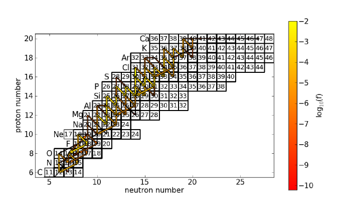
Figure 6: The network of 147 isotopes (H, He, Li, Be, and B isotopes are not plotted) used in our post-processing nucleosynthesis calculations. Reaction fluxes (arrows) correspond to our SPPN simulation for the dashed blue trajectory from upper panel of Fig. 1D to a moment when the temperature reaches its peak value of $T_{\mathrm{max}}=408$ MK (Table 1). The nucleosynthesis flux, $f=\delta Y_{\rm i}/\delta t_{\rm j}$, shows the variation rate of the abundance $Y_{\rm i}=X_{\rm i}/A_{\rm i}$ due to the reaction $j$. The arrow width and color correspond to the flux strength. Heavy-lined boxes correspond to the stable isotopes.

As a test of our MESA nova simulations, we have tried the MESA option for choosing the reaction rates that gives preference to the JINA Reaclib v1.1 (Cyburt et al., 2010), which includes the reaction rates evaluated by Iliadis et al. (2010). In spite of the presence of some differences in our nova $T_{\rm max}$-trajectories between the two options that preferentially choose the older (NACRE) and newer reaction rates (e.g., see the upper panel in Fig. 7 and compare the last two rows in Table 1), we have decided to use the default MESA option, as we did in Paper I. The switching between the two options is not likely to have a large effect on the nova hydrodynamic simulations but may impact nova nucleosynthesis. However, the latter is computed as post-processing of MESA nova models by the NuGrid code MPPNP that uses the most recent available reaction rates, including those from the JINA Reaclib.

In Fig. 7, upper panel, we show the $T_{\mathrm{max}}$-trajectories from two $1.3M_{\odot}$ ONe nova models with $T_{\mathrm{WD}}=20$ MK that accreted the pre-mixed material with the rate $\dot{M}=2\times 10^{-10}M_{\odot}/\mathrm{yr}$ for two different choices of reaction rate sources available in MESA, NACRE and JINA Reaclib. The two trajectories do not differ much from one another. In particular, their corresponding nuclear energy generation budget differs only by 16%.

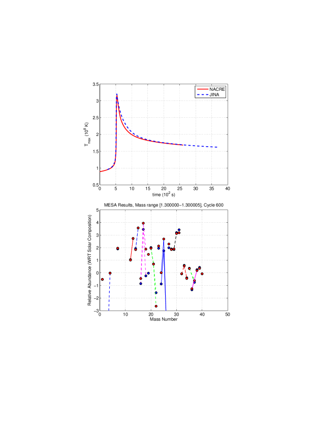
Figure 7: Upper panel: $T_{\rm max}$-trajectories from two $1.3\,M_{\odot}$ pre-mixed ONe nova models with $T_{\rm WD}=20$ MK and $\dot{M}=2\times 10^{-10}\,M_{\odot}/\mbox{yr}$ computed using the same largest nuclear network (nova.net) but different MESA reaction rate data, NACRE and JINA Reaclib. Lower panel: solar-scaled final abundances for these two models extracted from their MESA output files. Compare the red symbols from the lower panels in this figure and Fig. 8, the latter having been obtained in the post-processing nucleosynthesis computations with NuGrid’s MPPNP code.

The lower panel of Fig. 7 shows the production factors (mass fractions normalized to the solar composition) for stable isotopes whose abundances were averaged over the mass of the expanding nova envelope for the two discussed nova models. The nucleosynthesis yields are comparable in the two cases, with the largest differences for ²²Ne and Mg isotopes.

In Fig. 2, the results of our MPPNP simulations are shown for one of the CO nova models from Paper I for which a similar plot, but with data extracted from MESA simulations, was displayed in Fig. 5 of Paper I. Fig. 1 of José & Hernanz (1998) presents, in the same form, the nucleosynthesis yields for a CO nova model with the similar parameters. The data displayed in Fig. 2, Fig. 5 of Paper I, and Fig. 1 of José & Hernanz (1998) demonstrate a very good qualitative agreement, especially given that they were obtained with different nuclear networks, reaction rates, initial isotope abundances, and computer codes.

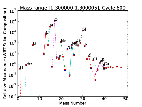
Figure 8: Solar-scaled final abundances from two $1.3\,M_{\odot}$ ONe nova models calculated using the largest (nova.net, red circles) and intermediate (nova_ONe.net, blue squares, the latter being overlapped by the red circles) nuclear networks. For these models, $T_{\rm WD}=20$ MK, and $\dot{M}=2\times 10^{-10}\,M_{\odot}/\mbox{yr}$.

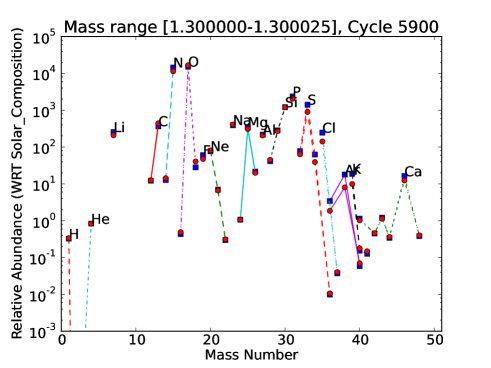
Figure 9: Same as in Fig. 8, but for $T_{\rm WD}=7$ MK, and $\dot{M}=10^{-11}\,M_{\odot}/\mbox{yr}$. $T_{\mathrm{max}}$-trajectories from these simulations are shown in Fig. 1D. For such extreme cases leading to the highest values of $T_{\mathrm{max}}$, the switching to the nova.net nuclear network is necessary.

The final abundances from four nova models are shown in Figs. 8 and 9. Two models are characterized by high WD temperature and relatively fast accretion, calculated using two different networks (nova.net and nova_ONe.net, Fig. 8). Their $T_{\mathrm{max}}$-trajectories (Fig. 1C) and final abundances (Fig. 8) are really similar. For the nova models with the coldest WDs and accreting with the slowest rates, the $T_{\mathrm{max}}$-trajectories are more different (Fig. 1D), although the relative nova yields do not show significant variations between the two cases (Fig. 9). In the upper panel of Fig. 10, we plot our final MPPNP abundances in the $1.3M_{\odot}$ ONe nova model with $T_{\mathrm{WD}}=12$ MK and $\dot{M}=2\times 10^{-10}M_{\odot}/\mathrm{yr}$. In this case, both the MESA and MPPNP simulations have used the Politano composition for the accreted material (the lower panel of Fig. 4). In the lower panel of Fig. 10, we show the ratios of our abundances to the corresponding final abundances from the ONe nova model I2005 that was computed by Starrfield et al. (2009) for the similar parameters, including the same pre-mixed initial composition. Most of the abundances agree with those of Starrfield et al. (2009) within a factor of ten. A similar comparison for our ONe nova model and its counterpart from José & Hernanz (1998) in Fig. 11, both computed with the Barcelona initial composition (the upper panel of Fig. 4), leads to the same conclusion. The final abundances from the two independent works with which we compare our results differ among each other as much as each differs from our results. A more detailed comparison would require simultaneous access to all participating simulation tools, and may not be justified given the present accuracy of available observable constraints.

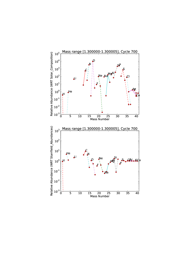
Figure 10: Upper panel: solar-scaled final abundances in the expanding envelope of our $1.3\,M_{\odot}$ ONe nova model with $T_{\rm WD}=12$ MK and $\dot{M}=2\times 10^{-10}\,M_{\odot}/\mbox{yr}$. The initial abundances for these simulations have been taken from Politano et al. (1995). Lower panel: the ratios of our final abundances to those reported by Starrfield et al. (2009) for a similar nova model with $M_{\rm WD}=1.35\,M_{\odot}$, $T_{\rm WD}=12$ MK, and $\dot{M}=1.6\times 10^{-10}\,M_{\odot}/\mbox{yr}$ (I2005A in their Table 5), who used the same initial abundances.

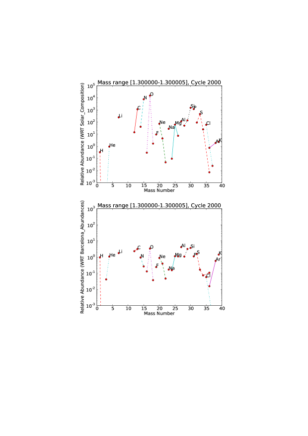
Figure 11: Same as in Fig. 10, but here we have used the Barcelona initial abundances and compare our MESA/NuGrid simulation results with those reported and plotted for a similar ONe nova model by José & Hernanz (1998) in their Table 3 (the ONe6 column) and Fig. 3.

Our MESA nova models with the CBM have also been post-processed with the MPPNP code, and the resulting final abundances are compared with those obtained for the corresponding nova models without CBM but with the pre-mixed accreted envelopes in the lower panels of Figs. 12 and 13 for the ONe and CO novae, respectively. The comparison between the final abundances shows a very good agreement for both the ONe and CO nova models. This gives a support to the widely-adopted 1D nova model in which the CBM is mimicked by assuming that the accreted envelope has been pre-mixed with the WD’s material.

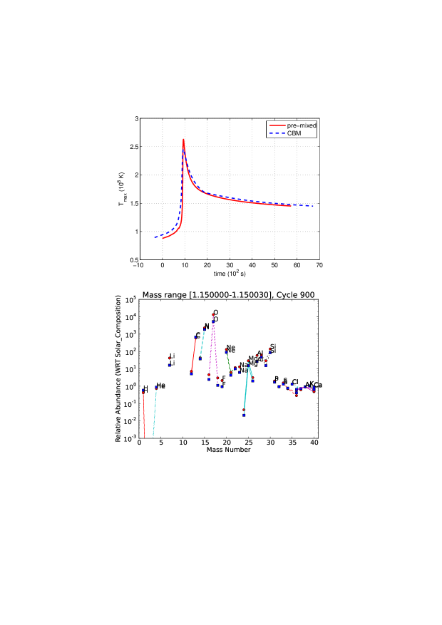
Figure 12: A comparison of $T_{\rm max}$-trajectories (the upper panel) and final abundances (the lower panel) from two of our $1.15\,M_{\odot}$ ONe nova simulations with $T_{\rm WD}=12$ MK and $\dot{M}=2\times 10^{-10}\,M_{\odot}/\mbox{yr}$. The solid red curve and red circles are the results obtained with the 50% pre-mixed initial abundances in the accreted envelope, while the dashed blue curve and blue squares represent the case with the solar-composition accreted material and convective boundary mixing (CBM) modeled using the same method and CBM parameter $f_{\rm nova}=0.004$ that we used in the $1.2\,M_{\odot}$ CO nova model in Paper I.

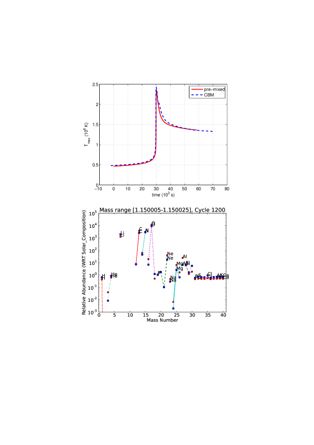
Figure 13: Same as in Fig. 12, but for the corresponding CO nova model.

Figure 14: A comparison of $T_{\rm max}$-trajectories (the upper panel) and solar-scaled final abundances (the lower panel) from three of our $1.3\,M_{\odot}$ pre-mixed ONe nova models computed for the same accretion rate, $\dot{M}=2\times 10^{-10}\,M_{\odot}/\mbox{yr}$, but different WD initial central temperatures (the symbols in the lower panel have the same color coding as their corresponding curves in the upper panel). The initial isotope abundances are those of the Barcelona group.

4.2 Single-Zone Computations: a Tool for Uncertainty and Sensitivity Studies

In this section, we discuss the post-processing simulations that use $T_{\mathrm{max}}$-trajectories extracted from the MESA $1.3M_{\odot}$ pre-mixed ONe nova models (shown in Fig. 14) with the mass accretion rate $\dot{M}=2\times 10^{-10}M_{\odot}/\mathrm{yr}$, but for the three different WD initial central temperatures, $T_{\mathrm{WD}}=12$, 15, and 20 MK . The accreted material had the Barcelona initial composition. The $T_{\mathrm{max}}$ peak values for these models are 344, 313, and 267 MK, respectively (Table 1). The post-processing nucleosynthesis calculations for these trajectories are performed using the NuGrid SPPN code. The solver and nuclear physics packages are the same that were used in our multi-zone post-processing nova computations (§4.1), and we use the same nuclear network with 147 isotopes (Fig. 6). The final abundance ratios for stable isotopes are presented in Fig. 15. The abundances were scaled using their corresponding solar values (the lower panel) as well as the results obtained for the WD model with $T_{\mathrm{WD}}=20$ MK (the upper panel).

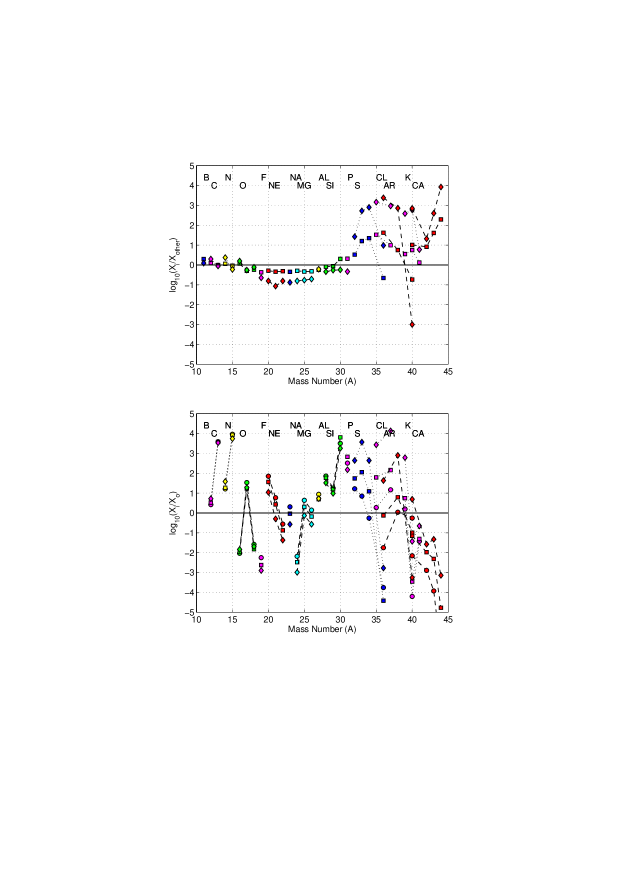
Figure 15: Lower panel: the final solar-scaled abundances of stable isotopes calculated with the SPPN code using the trajectories from the upper panel of Fig. 14 that correspond to the three different WD’s initial central temperatures: $T_{\mathrm{WD}}=12$ MK (diamonds), 15 MK (squares), and 20 MK (circles). Upper panel: the abundances from the first two sets are plotted as ratios with respect to the abundances from the last set. The unstable isotopes were allowed to decay.

A comparison between the abundance distributions in Figs. 15 and 14 shows a qualitative agreement between the results from the multi-zone complete models and from the single-zone $T_{\mathrm{max}}$-trajectories. Indeed, the abundance patterns for different groups of isotopes look similar. The main quantitative difference is the more efficient production toward heavier species in the second case, where O is more depleted, while Ar and K isotopes are more efficiently made. This difference is caused by the fact that in the multi-zone post-processing simulations convective mixing reduces an “average temperature” at which the nucleosynthesis occurs and it also constantly replenishes the hydrogen fuel burnt at the base of the envelope by bringing it from its outer parts, where $T\ll T_{\mathrm{max}}$. In general, the results in Fig. 15 show how the increase of the $T_{\mathrm{max}}$ peak value changes the relative abundance distribution. We conclude that SPPN nucleosynthesis simulations with nova $T_{\mathrm{max}}$-trajectories provide a proper qualitative indication of the behavior of their corresponding complete MPPNP simulations. However, they can be used only as a diagnostic for nova nucleosynthesis, e.g. in reaction rate sensitivity studies.

The nucleosynthesis in ONe novae and its sensitivity to reaction rates have been studied using post-processing (Iliadis et al., 2002) and full hydrodynamic (José & Hernanz, 2007; José et al., 2010) models. As a result, three reactions have been identified whose rate uncertainties have the most significant impact on models’ predictions: ¹⁸F(p,$\alpha)^{15}$O, ²⁵Al(p,$\gamma)^{26}$Si, and ³⁰P(p,$\gamma)^{31}$S.

The ¹⁸F(p,$\alpha)^{15}$O reaction rate is crucial for understanding the most intense 511 keV $\gamma$-ray emission that can be observed from novae, which is produced by positron annihilation associated with the decay of ¹⁸F. This nucleus is destroyed in a nova environment via ¹⁸F(p,$\alpha)^{15}$O. The uncertainty in the rate of this reaction therefore presents a limit to interpretation of any future observed $\gamma$-ray flux. This reaction rate has been evaluated recently in the compilation of Iliadis et al. (2010), where its uncertainty was about a factor of 2 over the temperature range characteristic of explosive hydrogen burning in novae. Since then, several experiments (Beer et al., 2011; Adekola et al., 2011; Mountford et al., 2012) have been performed to study the nuclear structure of the compound nucleus, ¹⁹Ne, above the proton threshold. As a result, this rate has been updated (Adekola et al., 2011), and its uncertainty has been reduced to a factor of 1.2 at 0.1 GK.

The ²⁵Al(p,$\gamma)^{26}$Si reaction rate was evaluated for the first time by Iliadis et al. (2001). Understanding this rate is important for an accurate prediction of the yield of ²⁶Al synthesized in ONe novae. The isotopic abundance ratio of ²⁶Al to ²⁷Al serves as a marker for identifying the candidate sources for presolar meteoritic grains. Due to the lack of knowledge of the properties of the proton resonances in ²⁶Si, the uncertainty in this rate at 0.1 – 0.4 GK ranges over 4 orders of magnitude (Iliadis et al., 2002). To reduce the uncertainty, the proton resonances in ²⁶Si have been studied experimentally, e.g. by Matic et al. (2010), Chen et al. (2012), and others, and, as a result, the most recent evaluation of the ²⁵Al(p,$\gamma)^{26}$Si rate by Jun Chen (2010, private communication) reports an uncertainty of about a factor of 670 over the temperature range of novae.

Finally, the reaction ³⁰P(p,$\gamma)^{31}$S drives the nuclear activity in ONe novae in the atomic mass region above $A=30$, and affects the isotopic abundance ratio of ³⁰Si to ²⁸Si, which in turn helps identify novae as a potential origin for some SiC presolar grains. Its rate was first estimated by Rauscher & Thielemann (2000) via Hauser-Feschbach statistical calculations, and was further discussed in Iliadis et al. (2001). The properties of the proton resonances in ³¹S were also largely unknown at the time, and therefore, this rate too suffered from an uncertainty ranging over 4 orders of magnitude for nova temperatures (Iliadis et al., 2002). In recent years, the nuclear structure of ³¹S has been studied extensively (Ma et al., 2007; Wrede et al., 2009; Parikh et al., 2011; Doherty et al., 2012), and now the most updated rate has an uncertainty of a factor of $\sim 17$ at 0.3 GK (Parikh et al., 2011).

We have calculated the effect of uncertainties in the rates of two of the aforementioned nuclear reactions on final nova abundances with the NuGrid SPPN code. In order to estimate the maximum effect, we have used the $T_{\mathrm{WD}}=12$ MK trajectory from the upper panel of Fig. 14 that has the highest value of $T_{\mathrm{max}}=344$ MK. Figs. 16 and 17 show the final relative abundances of stable isotopes resulting from varying the ²⁵Al(p,$\gamma)^{26}$Si and ³⁰P(p,$\gamma)^{31}$S reaction rates, respectively, within their (largest) 4 orders of magnitude uncertainties used by Iliadis et al. (2002). Our results in Fig. 17 are in good agreement with those presented by Iliadis et al. (2002) in their Fig. 3d. In particular, for both the sensitivity studies the final abundances are more affected by reducing the rates considered, starting respectively from ²⁸Si and ³⁰Si.

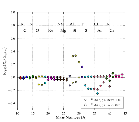
Figure 16: Comparison of the final abundances of stable isotopes calculated with the SPPN code using the $T_{\mathrm{WD}}=12$ MK trajectory from the upper panel of Fig. 14 for the recommended set of reaction rates ($X_{\mathrm{other}}$) with the abundances ($X_{i}$) obtained with the rate of the reaction ²⁵Al(p,$\gamma)^{26}$Si increased (circles) and decreased (diamonds) by the factor of 100, like in the nuclear sensitivity study of Iliadis et al. (2002).

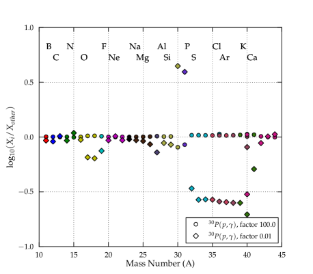
Figure 17: Same as in Fig. 16, but for the reaction ³⁰P(p,$\gamma)^{31}$S.

The destruction of ²⁵Al is mainly due to the ²⁵Al($\beta$⁺)²⁵Mg and ²⁵Al(p,$\gamma)^{26}$Si reactions. Reducing the ²⁵Al(p,$\gamma)^{26}$Si, the nucleosynthesis path synthesizes less ²⁶Si and ²⁷P, therefore reducing the flux through this nucleosynthesis channel. On the other hand, ²⁵Al is accumulated causing a more efficient decay to ²⁵Mg. Starting from ²⁵Mg, the proton capture chain ²⁵Mg(p,$\gamma)^{26}$Al(p,$\gamma)^{27}$Si(p,$\gamma)^{28}$P($\beta$⁺)²⁸Si causes a higher ²⁸Si production. However, the suppression of the ²⁵Al(p,$\gamma)^{26}$Si channel makes the proton capture nucleosynthesis overall slower, reducing the production in the heavier S-Cl region and increasing the yields of Si and P in the final nova ejecta.

The ³⁰P(p,$\gamma)^{31}$S reaction is the dominant destruction channel for ³⁰P. Therefore, reducing its rate makes ³⁰P a bottleneck for further proton-capture nucleosynthesis, reducing the production of heavier species. The isotope ³⁰P is accumulated, and also ³⁰Si via ³⁰P($\beta$⁺)³⁰Si. As a result, more ³⁰Si and ³¹P are made, and less between S and ⁴⁰Ca.

The differences between the final nova abundances caused by the variations of the reaction rates are much smaller than those obtained for the slightly different WD’s initial central temperatures in Fig. 15. Therefore, these nuclear uncertainty studies for novae are particularly important for detailed comparisons of the isotopic composition in a given atomic mass range, e.g. from presolar grain measurements.

Note that these tests based on changing a single reaction rate are quite common in nuclear astrophysics studies. This needs to be done carefully, since a consistent uncertainty study for nuclear reaction rates of the nearby species should also be included. It is not the purpose of this section to carry out such a detailed analysis for ²⁵Al(p,$\gamma)^{26}$Si and ³⁰P(p,$\gamma)^{31}$S. The point that we wanted to stress here is that single-zone trajectories can be used as tools for exploratory studies to identify which reactions are relevant for the nucleosynthesis (i.e., for sensitivity studies), and within which errors reaction rates are needed to not affect stellar abundance predictions (i.e., for uncertainty studies).

5 Effects Caused by ³He Burning

In Paper I, we have found, for the first time, that in the extreme case of a very cold CO WD, e.g. with $T_{\mathrm{WD}}=7$ MK, accreting solar-composition material with a very low rate, say $\dot{M}=10^{-11}M_{\odot}/\mathrm{yr}$, the incomplete pp I chain reactions lead to the in situ synthesis of ³He in a slope adjacent to the base of the accreted envelope and that the ignition of this ³He triggers convection before the major nova outburst. The ³He burning continues at a relatively low temperature, $T\approx 30$ MK, approximately until its abundance is reduced below the solar value, only after that the major nova outburst ensues triggered by the reaction ¹²C(p,$\gamma)^{13}$N. Although this is an interesting variation of the nova scenario, because the CO enrichment of the accreted envelope is produced by the ³He-driven CBM in this case, its observational frequency is expected to be very low (Paper I). Here, we confirm this result for ONe novae (Fig. 18). Furthermore, we have found that in the $1.15\,M_{\odot}$ ONe WD with a relatively high initial central temperature, $T_{\rm WD}=15$ MK, accreting the solar-composition material with the intermediate rate, $\dot{M}=10^{-10}\,M_{\odot}/\mbox{yr}$, the interplay between the ³He production and destruction in the vicinity of the base of the accreted envelope first leads to a shift of $T_{\mathrm{max}}$ away from the core-envelope interface followed by the formation of a thick radiative buffer zone that separates the bottom of the convective envelope from the WD surface (Fig. 19). This result is obtained only for the case when an ONe WD accretes solar-composition material and it almost disappears in the models with the pre-mixed accreted envelopes. Given that the formation of the radiative buffer zone is revealed in the computations with the more realistic nova model parameters, such cases can probably be observed. We defer a more detailed study of this peculiar case and its possible consequences to a future work. In particular, it would be interesting to see if the CBM can cross the buffer zone and reach the WD core.

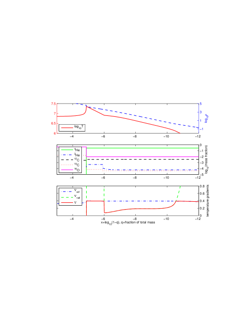
Figure 18: A snapshot of profiles of relevant stellar structure parameters in the envelope of our $1.3\,M_{\odot}$ ONe nova model with $T_{\rm WD}=7$ MK and $\dot{M}=10^{-11}\,M_{\odot}/\mbox{yr}$ at the moment following the ³He ignition that has triggered convection. Like in the CO nova model with the cold WD and low accretion rate discussed in Paper I, the low $T_{\rm WD}$ and $\dot{M}$ values favour the accumulation of ³He in a slope adjacent to the core-envelope interface followed by its ignition at a relatively low $T$, before the major thermonuclear runaway ensues.

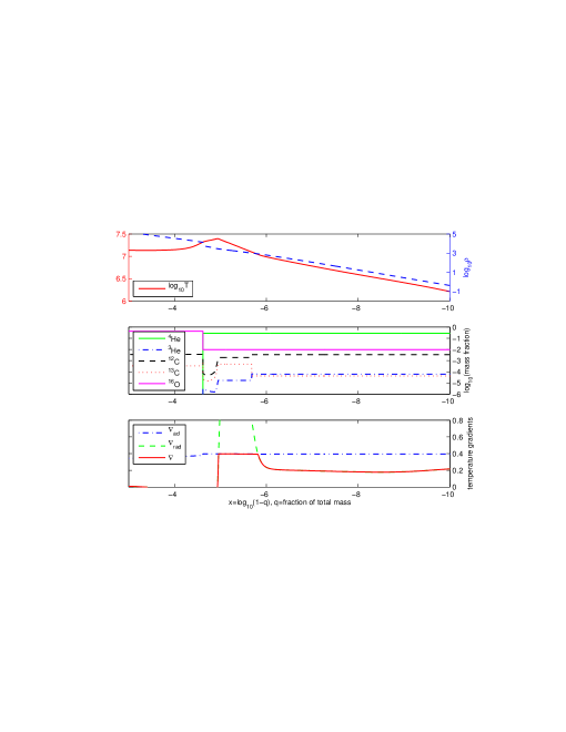
Figure 19: A snapshot similar to that shown in Fig. 18, but for our $1.15\,M_{\odot}$ ONe nova model with $T_{\rm WD}=15$ MK and $\dot{M}=10^{-10}\,M_{\odot}/\mbox{yr}$. The interplay between the ³He production and destruction shifts the peak temperature away from the core-envelope interface, located at the leftmost steps on the abundance profiles (the middle panel), to a place where the ³He burning generates the maximum energy. This leads to the formation of a convective zone separated from the interface by a buffer zone. Note that this model and the one in Fig. 18 accrete solar-composition material.

6 Comparison With Observed Chemical Compositions of Novae

6.1 Element Abundances From Optical, Ultraviolet and Infrared Spectroscopy

Difficulties with determining element abundances from the spectra of nova ejecta are discussed by Gehrz et al. (1998). The same authors have compiled the largest set of mass fractions of H, He, and heavy elements, such as C, N, O, Ne, in novae from optical and ultraviolet spectroscopy that were published in the period from 1978 until 1997. In Fig. 20, we compare these abundances (the filled red star symbols) as well as ONe nova abundances from the recent compilation by Downen et al. (2013, the open black star symbols), that include infrared spectroscopy data, with the corresponding nucleosynthesis yields predicted by our $1.15M_{\odot}$ pre-mixed nova models from Figs. 12 and 13. We also include the abundance predictions by José & Hernanz (1998). For each of the novae listed in Table 2 of Gehrz et al. (1998), we have used all the available abundance measurements, therefore some of the novae are represented by up to three points for the same element in our Fig. 20 that correspond to different data sources. We have divided the observed objects into CO (panel A) and ONe (panel B) novae using the neon mass fraction ratios $X(\mathrm{Ne})/X_{\odot}(\mathrm{Ne})<8$ and $X(\mathrm{Ne})/X_{\odot}(\mathrm{Ne})>10$ for the first and second group. Neither panel shows a good agreement between the observed and predicted element abundances for the novae, because both show the presence of large numbers of observed objects with too low C and O abundances as compared to the model predictions. The latter rather represent upper limits for the observed data. We do not know how to interpret this discrepancy, other than to assume that the observed material has been mixed with the solar-composition material from the WD’s companion. We have tried to reduce the amount of CO WD’s material in the pre-mixed accreted envelope from 50% to 25% but this does not help much (compare the solid and dashed blue curves in the panel A). Note that our model predictions almost coincide with those of the Barcelona group in Fig. 20.

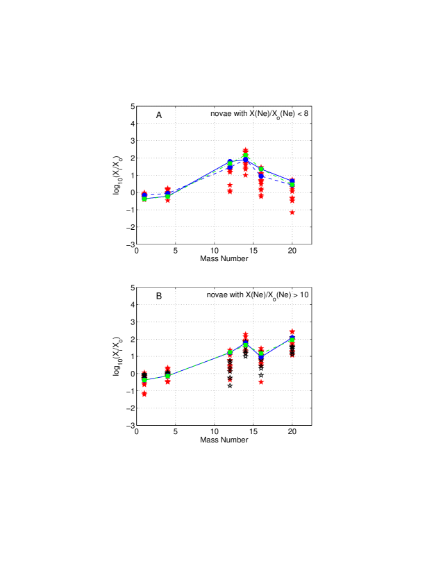
Figure 20: Comparison of the H, He, C, N, O, and Ne mass fractions in novae from optical, ultraviolet and infrared spectroscopy (the filled red and open black star symbols are data from Gehrz et al. 1998 and Downen et al. 2013, respectively) with the theoretical ones obtained in nova simulations. Blue circles connected by solid blue curves in panels A and B correspond to our CO and ONe nova models with 50% pre-mixed accreted envelopes from Figs. 13 and 12. The dashed blue curve in panel A represents our results for a 25% pre-mixed CO nova model, while green squares connected by dot-dashed green curves in panels A and B are data for nova models, CO5 and ONe3, from Tables 4 and 3 of José & Hernanz (1998).

6.2 Presolar Grains

Absorption features due to carbide grains have been observed around novae (e.g., Starrfield et al., 1997; Gehrz et al., 1998). This opens a possibility to find in the solar system, hidden in carbonaceous pristine meteorites, presolar grains that condensed around nova objects shortly before the Sun formed, and possibly carrying the Ne-E component observed in meteoritic samples (Starrfield et al., 1997). This scenario is confirmed by the analysis of abundances for a small fraction of presolar grains identified so far, which show distinctive isotopic signatures that may be associated with nova nucleosynthesis: a minor fraction of the presolar silicon carbides (SiC nova, Amari et al., 2001; Amari, 2002; José & Hernanz, 2007; Heck et al., 2007), a few graphite grains (e.g., Amari et al., 2001; Zinner et al., 2007), and oxides (e.g., Gyngard et al., 2010; Nittler et al., 2010; Gyngard et al., 2011). Oxide grains should form in CO novae, whereas carbide grains around ONe novae, since the ejected material shows the C to O abundance ratios less than unity in the first case, and being C-rich in the last case (e.g., Amari et al. 2001; also, see our Table 2). However, observational features of carbide dust have been observed also around CO novae, and therefore this simple distinction cannot be made (Gehrz, 2002). The distinctive isotopic signatures of nova grains include extremely high excesses of ¹³C, ¹⁵N, overabundances of ²⁶Mg and ²²Ne due to the later radiogenic decay of the radioactive ²⁶Al and ²²Na (Table 2), and high ¹⁷O/¹⁶O isotopic ratios, specifically for oxide grains (Clayton & Hoyle, 1976; Amari et al., 2001; Amari, 2002; José & Hernanz, 2007). Nittler & Hoppe (2005) suggested that, at least, part of the nova SiC grains are instead made from material ejected by core-collapse SNe, showing typical nova signatures coupled with ²⁸Si and ⁴⁴Ti excesses that cannot be obtained from novae.

Table 2: Comparison of Selected Abundances in Pre-Mixed Nova Models^a

Abundance	Fig. 1	CO5	Fig. 14	ONe3	Fig. 13	ONe6
$\mathrm{C}/\mathrm{O}$	0.56	0.78	0.36	0.43	2.2	1.2
$X_{22}$	$6.1\times 10^{-7}$	$2.9\times 10^{-7}$	$2.6\times 10^{-4}$	$5.3\times 10^{-5}$	$1.1\times 10^{-3}$	$6.0\times 10^{-4}$
$X_{26}$	$2.1\times 10^{-4}$	$4.7\times 10^{-5}$	$3.1\times 10^{-4}$	$9.3\times 10^{-4}$	$8.4\times 10^{-4}$	$7.2\times 10^{-4}$

^aThe C to O number ratios and mass fractions of ²²Na and ²⁶Al are taken from our models shown in the indicated figures and from Tables 3 and 4 of José & Hernanz (1998) for their corresponding counterparts that are denoted by CO5, ONe3, and ONe6.

In this section, we compare the model results presented in the previous sections for ONe novae with presolar SiC grains. Also plotted are the results for CO novae from Paper I. We derive a single data point for the isotope abundances from each nova model, using the mass average of all zones in the last time step of post-processing nucleosynthesis simulations, and use these data to compare stellar model predictions with isotopic ratios measured in presolar grains. We assume that all the zones in the expanding envelope will eventually be ejected after its radius has reached a few solar radii. We do not distinguish between carbon and oxygen rich layers in the expanding nova envelope. This results in an average isotopic composition for each individual nova simulation and does not necessarily represent what presolar grain incorporate. A more detailed comparison between grains of possible nova origin and ejected layers with nova models would require a dedicated investigation. Figs. 21 and 22 compare presolar SiC nova grains with our model results. For presolar grains, we used the Washington University (St. Louis) database for data extraction (Hynes & Gyngard, 2009). The data mostly fall between the model and average solar system isotopic ratios. Therefore, present models reproduce the data well, if some contamination with solar system material is taken into account. Sample contamination either happened on the asteroid parent body or in the lab. Since no major and minor element concentrations were measured in the grains, a mixing calculation cannot be performed here.

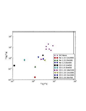
Figure 21: Comparison of the C and N isotopic ratios from our ONe and CO nova models with presolar grain data. Black lines indicate the solar system values. Presolar grain data are from Amari et al. (2001); Gao & Nittler (1997); Hoppe et al. (1996); Nittler & Hoppe (2005). Nova models are denoted by their composition (Ne or CO), WD mass ($M_{\odot}$) and initial central temperature (MK), followed by a number of models in the evolutionary sequence. Their expanding envelopes are mixed as described in the text.

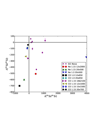
Figure 22: Comparison of the Si isotopic ratios from ONe and CO nova models with single presolar grain data. For the isotopic ratios, the delta notations are used ($\delta$(ratio) = (stellar ratio/solar ratio - 1)$\times$1000). Black lines indicate the solar system values. The presolar grain data are from Amari et al. (2001); Gao & Nittler (1997); Hoppe et al. (2010); Nittler & Alexander (2003); Nittler & Hoppe (2005). Nova models are denoted by their composition (Ne or CO), WD mass ($M_{\odot}$) and initial central temperature (MK), followed by a number of models in the evolutionary sequence. Their expanding envelopes are mixed as described in the text.

Equilibrium condensation calculations show that SiC grains are only expected to condense in environments where the C/O ratio is larger than one (see, e.g., Zinner, 2003). Therefore, unless mixing of the ejecta takes place, the chosen approach to mix all shells together, is not completely valid. Fig. 23 shows the evolution of the C/O elemental ratio in the ONe nova models (upper panel) and CO nova models from Paper I (lower panel). To make changes on the surface visible and plot all models in one graph, the mass layers were normalized from zero to one and inverted, such that the outermost shell plots on the left side. Only part of the nova ejecta is C-rich. Without a clear mixing prescription for the ejecta – if existing – a definite comparison with presolar grains requires a careful study where the analysis is performed grain-by-grain, and considering the isotopic signature in different stellar zones.

In summary, we find a general agreement between our nucleosynthesis calculation trends and isotopic abundance measurements from SiC grains with a possible nova origin. The comparison however only gives a trend of our nova models since mixing in the ejecta and contamination with solar system material have to be further taken into account and discussed. A more detailed grain-by-grain analysis is required for a consistent and constraining analysis, including analyses of more isotopic constraints where available.

Figure 23: C/O ratios in expanding envelopes of all nova models in the last time step. The C/O = 1 is indicated by a straight line in each plot. To plot all models on the same mass scale and point out differences in the outer layers better, the x-axis shows the mass-shell for each model normalized from 0 to 1 and inverted. This means that the outermost shell lies on the left side, while the innermost shell is on the right. The figure clearly demonstrates that mixing of the whole envelope is not a priori valid, rather carbon rich zones have to be mixed and analyzed in order to obtain a valid comparison with presolar SiC grains.

7 Conclusion

We have created the Nova Framework that allows to simulate the accretion of H-rich material onto a white dwarf (WD) leading, for a suitable set of initial parameters, to a nova outburst, and to post-process its accompanying nucleosynthesis. The Nova Framework combines the state-of-the-art stellar evolution code MESA and post-processing nucleosynthesis tools of NuGrid. It includes a number of CO and ONe WD models with different masses and central temperatures (luminosities) that can be used in simulations of nova outbursts. The use of the Nova Framework is facilitated by a number of shell scripts that carry out the routine job necessary to coordinate the operation of the MESA and NuGrid codes.

Within the Nova Framework effort, we provide a large set of nucleosynthesis calculations for nearly 50 CO and ONe nova models at the solar metallicity ($Z=0.02$) so far. To verify our calculations, we compare their results with those published in the literature for similar nova models. The comparison shows a very good qualitative agreement analogous to the case when different nova yields from the literature are compared with each other. Typical features of abundance signatures of novae from previous studies and observations are confirmed. For instance, the large production factors for ¹³C, ¹⁵N, and ¹⁷O in both CO and ONe novae, the synthesis of ⁷Li in CO novae, the overabundance of Ne as a distinctive feature of ONe novae, as well as the accumulation of relatively large mass fractions of the radioactive isotopes ²²Na and ²⁶Al in ONe novae (unfortunately, not detected by $\gamma$ telescopes yet).

The nucleosynthesis in novae is studied using the post-processing method. We show that such a technique provides abundance predictions consistent with stellar model calculations. We study the impact on the final abundances of model parameters relevant for novae, such as the mass, composition and initial central temperature of the underlying WD, and the mass accretion rate. In particular, decreasing the initial central temperature causes the outburst peak temperature to increase, which in turn enhances the production of isotopes in the region between Si and Ca. The main effect of the decrease of the accretion rate is an increase of the envelope mass $M_{\mathrm{acc}}$ accreted before a nova outburst. The higher $M_{\mathrm{acc}}$ value results in a stronger explosion with a higher peak temperature. For accretion of solar-composition material with a very low rate, e.g. $\dot{M}=10^{-11}M_{\odot}/\mathrm{yr}$, onto a very cold WD, e.g. with $T_{\mathrm{WD}}=7$ MK, we find the in situ synthesis of ³He taking place via the incomplete pp I chain near the bottom of the accreted envelope. The ignition and burning of this ³He at a relatively low temperature ($T\sim 30$ MK) triggers convection in the envelope before the major nova outburst, the latter ensuing only after the ³He abundance has been reduced below its solar value. We demonstrate that this happens not only in CO novae (Paper I) but also in ONe novae. Moreover, we reveal that the interplay between the ³He production and destruction in the solar-composition envelope accreted with an intermediate rate, e.g. $\dot{M}=10^{-10}\,M_{\odot}/\mbox{yr}$, by the $1.15\,M_{\odot}$ ONe WD with a relatively high initial central temperature, e.g. $T_{\rm WD}=15\times 10^{6}$ K, leads to the formation of a thick radiative buffer zone that separates the bottom of the convective envelope from the WD surface.

We use three $T_{\mathrm{max}}$-trajectories, extracted from full nova models, in single-zone post-processing nucleosynthesis computations with the NuGrid SPPN code. We show that the results obtained in the one-zone simulations are qualitatively consistent with the yields from complete models post-processed with the NuGrid multi-zone code MPPNP, including the impact of stellar parameters, like the WD initial central temperature. Therefore, simple trajectories can be used as important diagnostic tools for nova nucleosynthesis, e.g., for nuclear sensitivity and uncertainty studies. As example, we have studied the impact on nova nucleosynthesis of the ²⁵Al(p,$\gamma)^{26}$Si and ³⁰P(p,$\gamma)^{31}$S reaction rates. In particular, we find that abundance predictions are more affected by reducing those rates.

The interested reader can try to post-process our nova $T_{\mathrm{max}}$-trajectories with the NuGrid SPPN code using our NuGrid Ubuntu ppn-nova virtual machine. Instructions on how to use this virtual machine can be found on http://nugridstars.org in the subsection “Virtual Box releases” of the section “Releases and Software Downloads”.

References

- Adekola et al. (2011) Adekola A. S., Bardayan D. W., Blackmon J. C., et al. 2011, Phys. Rev. C, 83, 052801
- Amari (2002) Amari S., 2002, New A. Rev., 46, 519
- Amari et al. (2001) Amari S., Gao X., Nittler L. R., Zinner E., José J., Hernanz M., Lewis R. S., 2001, ApJ, 551, 1065
- Angulo et al. (1999) Angulo C., Arnould M., Rayet M., et al. 1999, Nuclear Physics A, 656, 3
- Arnett & Truran (1969) Arnett W. D., Truran J. W., 1969, ApJ, 157, 339
- Beer et al. (2011) Beer C. E., Laird A. M., Murphy A. S. J., Bentley M. A., Buchman L., Davids B., Davinson T., Diget C. A., Fox S. P., Fulton B. R., Hager U., Howell D., Martin L., Ruiz C., Ruprecht G., Salter P., Vockenhuber C., Walden P., 2011, Phys. Rev. C, 83, 042801
- Casanova et al. (2010) Casanova J., José J., García-Berro E., Calder A., Shore S. N., 2010, A&A, 513, L5
- Casanova et al. (2011) Casanova J., José J., García-Berro E., Shore S. N., Calder A. C., 2011, Nature, 478, 490
- Caughlan & Fowler (1988) Caughlan G. R., Fowler W. A., 1988, Atomic Data and Nuclear Data Tables, 40, 283
- Chen et al. (2012) Chen J., Chen A. A., Amthor A. M., Bazin D., Becerril A. D., Gade A., Galaviz D., Glasmacher T., Kahl D., Lorusso G., Matos M., Ouellet C. V., Pereira J., Schatz H., Smith K., Wales B., Weisshaar D., Zegers R. G. T., 2012, Phys. Rev. C, 85, 045809
- Chen et al. (2013) Chen M. C., Herwig F., Denissenkov P. A., Paxton B., 2013, ArXiv e-prints
- Clayton & Hoyle (1976) Clayton D. D., Hoyle F., 1976, ApJ, 203, 490
- Cyburt et al. (2010) Cyburt R. H., Amthor A. M., Ferguson R., Meisel Z., Smith K., Warren S., Heger A., Hoffman R. D., Rauscher T., Sakharuk A., Schatz H., Thielemann F. K., Wiescher M., 2010, ApJS, 189, 240
- Denissenkov et al. (2013) Denissenkov P. A., Herwig F., Bildsten L., Paxton B., 2013, ApJ, 762, 8
- Denissenkov et al. (2013) Denissenkov P. A., Herwig F., Truran J. W., Paxton B., 2013, ApJ, 772, 37
- Doherty et al. (2012) Doherty D. T., Lotay G., Woods P. J., Seweryniak D., Carpenter M. P., Chiara C. J., David H. M., Janssens R. V. F., Trache L., Zhu S., 2012, Phys. Rev. Lett., 108, 262502
- Downen et al. (2013) Downen L. N., Iliadis C., José J., Starrfield S., 2013, ApJ, 762, 105
- Freytag et al. (1996) Freytag B., Ludwig H.-G., Steffen M., 1996, A&A, 313, 497
- Fuller (1985) Fuller E. G., 1985, Phys. Rep., 127, 185
- Fynbo et al. (2005) Fynbo H. O. U., Diget C. A., Bergmann U. C., et al. ISOLDE Collaboration 2005, Nature, 433, 136
- Gao & Nittler (1997) Gao X., Nittler L. R., 1997, in Lunar and Planetary Institute Science Conference Abstracts Vol. 28 of Lunar and Planetary Inst. Technical Report, Si-30-enriched presolar SiC in ACFER 094. p. 393
- Gehrz (2002) Gehrz R. D., 2002, in Hernanz M., José J., eds, Classical Nova Explosions Vol. 637 of American Institute of Physics Conference Series, Infrared and Radio Observations of Classical Novae: Physical Parameters and Abundances in the Ejecta. pp 198–207
- Gehrz et al. (1998) Gehrz R. D., Truran J. W., Williams R. E., Starrfield S., 1998, PASP, 110, 3
- Gil-Pons et al. (2003) Gil-Pons P., García-Berro E., José J., Hernanz M., Truran J. W., 2003, A&A, 407, 1021
- Glasner et al. (1997) Glasner S. A., Livne E., Truran J. W., 1997, ApJ, 475, 754
- Glasner et al. (2005) Glasner S. A., Livne E., Truran J. W., 2005, ApJ, 625, 347
- Glasner et al. (2012) Glasner S. A., Livne E., Truran J. W., 2012, MNRAS, 427, 2411
- Goriely (1999) Goriely S., 1999, A&A, 342, 881
- Görres et al. (2000) Görres J., Arlandini C., Giesen U., Heil M., Käppeler F., Leiste H., Stech E., Wiescher M., 2000, Phys. Rev. C, 62, 055801
- Grevesse & Noels (1993) Grevesse N., Noels A., 1993, in Prantzos N., Vangioni-Flam E., Casse M., eds, Origin and Evolution of the Elements Cosmic abundances of the elements.. pp 15–25
- Gyngard et al. (2011) Gyngard F., Nittler L. R., Zinner E., Jose J., Cristallo S., 2011, in Lunar and Planetary Institute Science Conference Abstracts Vol. 42 of Lunar and Planetary Institute Science Conference Abstracts, New Reaction Rates and Implications for Nova Nucleosynthesis and Presolar Grains. p. 2675
- Gyngard et al. (2010) Gyngard F., Zinner E., Nittler L. R., Morgand A., Stadermann F. J., Mairin Hynes K., 2010, ApJ, 717, 107
- Heck et al. (2007) Heck P. R., Marhas K. K., Hoppe P., Gallino R., Baur H., Wieler R., 2007, ApJ, 656, 1208
- Herwig et al. (1997) Herwig F., Bloecker T., Schoenberner D., El Eid M., 1997, A&A, 324, L81
- Herwig et al. (2008) Herwig F., Diehl S., Fryer C. L., Hirschi R., Hungerford A., Magkotsios G., Pignatari M., Rockefeller G., Timmes F. X., Young P., Bennet M. E., 2008, in Nuclei in the Cosmos (NIC X) Nucleosynthesis simulations for a wide range of nuclear production sites from NuGrid
- Hoppe et al. (1996) Hoppe P., Kocher T. A., Strebel R., Eberhardt P., Amari S., Lewis R. S., 1996, in Lunar and Planetary Institute Science Conference Abstracts Vol. 27 of Lunar and Planetary Inst. Technical Report, Origin of Circumstellar SiC Grains With Low 12C/13C Ratios: A Multiple Star Scenario. p. 561
- Hoppe et al. (2010) Hoppe P., Leitner J., Gröner E., Marhas K. K., Meyer B. S., Amari S., 2010, ApJ, 719, 1370
- Hynes & Gyngard (2009) Hynes K. M., Gyngard F., 2009, in Lunar and Planetary Institute Science Conference Abstracts Vol. 40 of Lunar and Planetary Inst. Technical Report, The Presolar Grain Database: http://presolar.wustl.edu/~pgd. p. 1198
- Iliadis et al. (2002) Iliadis C., Champagne A. E., J. José J., Starrfield S., Tupper P., 2002, ApJS, 142, 105
- Iliadis et al. (2001) Iliadis C., D’Auria J. M., Starrfield S., Thompson W. J., Wiescher M., 2001, ApJS, 134, 151
- Iliadis et al. (2010) Iliadis C., Longland R., Champagne A. E., Coc A., Fitzgerald R., 2010, Nuclear Physics A, 841, 31
- Imbriani et al. (2005) Imbriani G., Costantini H., Formicola A., et al. 2005, European Physical Journal A, 25, 455
- José et al. (2010) José J., Casanova J., Moreno F., García-Berro E., Parikh A., Iliadis C., 2010, in Tours Symposium on Nuclear Physics and Astrophysics VII Vol. 1238 of AIP Conf. Proc., Hydrodynamic Models of Classical Novae and Type I X-Ray Bursts. pp 157–162
- José et al. (1999) José J., Coc A., Hernanz M., 1999, ApJ, 520, 347
- José et al. (2001) José J., Coc A., Hernanz M., 2001, ApJ, 560, 897
- José et al. (2007) José J., García-Berro E., Hernanz M., Gil-Pons P., 2007, ApJ, 662, L103
- José & Hernanz (1998) José J., Hernanz M., 1998, ApJ, 494, 680
- José & Hernanz (2007) José J., Hernanz M., 2007, Journal of Physics G Nuclear Physics, 34, 431
- Kercek et al. (1998) Kercek A., Hillebrandt W., Truran J. W., 1998, A&A, 337, 379
- Kunz et al. (2002) Kunz R., Fey M., Jaeger M., Mayer A., Hammer J. W., Staudt G., Harissopulos S., Paradellis T., 2002, ApJ, 567, 643
- Langanke & Martínez-Pinedo (2000) Langanke K., Martínez-Pinedo G., 2000, Nuclear Physics A, 673, 481
- Livio & Truran (1994) Livio M., Truran J. W., 1994, ApJ, 425, 797
- Lodders (2003) Lodders K., 2003, ApJ, 591, 1220
- Ma et al. (2007) Ma Z., Bardayan D. W., Blackmon J. C., Fitzgerald R. P., Guidry M. W., Hix W. R., Jones K. L., Kozub R. L., Livesay R. J., Smith M. S., Thomas J. S., Visser D. W., 2007, Phys. Rev. C, 76, 015803
- Matic et al. (2010) Matic A., van den Berg A. M., Harakeh M. N., et al. 2010, Phys. Rev. C, 82, 025807
- Mountford et al. (2012) Mountford D. J., Murphy A. S. J., Achouri N. L., Angulo C., Brown J. R., Davinson T., de Oliveira Santos F., de Séréville N., Descouvemont P., Kamalou O., Laird A. M., Pittman S. T., Ujic P., Woods P. J., 2012, Phys. Rev. C, 85, 022801
- Nittler & Alexander (2003) Nittler L. R., Alexander C. M. O., 2003, Geochim. Cosmochim. Acta, 67, 4961
- Nittler et al. (2010) Nittler L. R., Gyngard F., Zinner E., 2010, Meteoritics and Planetary Science Supplement, 73, 5245
- Nittler & Hoppe (2005) Nittler L. R., Hoppe P., 2005, ApJ, 631, L89
- Oda et al. (1994) Oda T., Hino M., Muto K., Takahara M., Sato K., 1994, Atomic Data and Nuclear Data Tables, 56, 231
- Paczyński (1970) Paczyński B., 1970, Acta Astron., 20, 47
- Parikh et al. (2011) Parikh A., Wimmer K., Faestermann T., Hertenberger R., José J., Longland R., Wirth H.-F., Bildstein V., Bishop S., Chen A. A., Clark J. A., Deibel C. M., Herlitzius C., Krücken R., Seiler D., Straub K., Wrede C., 2011, Phys. Rev. C, 83, 045806
- Paxton et al. (2011) Paxton B., Bildsten L., Dotter A., Herwig F., Lesaffre P., Timmes F., 2011, ApJS, 192, 3
- Paxton et al. (2013) Paxton B., Cantiello M., Arras P., Bildsten L., Brown E. F., Dotter A., Mankovich C., Montgomery M. H., Stello D., Timmes F. X., Townsend R., 2013, ArXiv e-prints
- Pignatari & Herwig (2012) Pignatari M., Herwig F., 2012, Nuclear Physics News, 22, 18
- Politano et al. (1995) Politano M., Starrfield S., Truran J. W., Weiss A., Sparks W. M., 1995, ApJ, 448, 807
- Prialnik & Kovetz (1995) Prialnik D., Kovetz A., 1995, ApJ, 445, 789
- Rauscher & Thielemann (2000) Rauscher T., Thielemann F.-K., 2000, At. Data Nucl. Data Tables, 75, 1
- Ritossa et al. (1996) Ritossa C., Garcia-Berro E., Iben Jr. I., 1996, ApJ, 460, 489
- Schatzman (1951) Schatzman E., 1951, Annales d’Astrophysique, 14, 294
- Shara (1989) Shara M. M., 1989, PASP, 101, 5
- Starrfield (1989) Starrfield S., 1989, in Bode M. F., Evans A., eds, Classical Novae Thermonuclear processes and the classical nova outburst.. pp 39–60
- Starrfield et al. (1997) Starrfield S., Gehrz R. D., Truran J. W., 1997, in Bernatowicz T. J., Zinner E., eds, American Institute of Physics Conference Series Vol. 402 of American Institute of Physics Conference Series, Dust formation and nucleosynthesis in the nova outburst. pp 203–234
- Starrfield et al. (2009) Starrfield S., Iliadis C., Hix W. R., Timmes F. X., Sparks W. M., 2009, ApJ, 692, 1532
- Townsley & Bildsten (2004) Townsley D. M., Bildsten L., 2004, ApJ, 600, 390
- Truran (1982) Truran J. W., 1982, in Barnes C. A., Clayton D. D., Schramm D. N., eds, Essays in Nuclear Astrophysics Nuclear Theory of Novae. p. 467
- Truran & Livio (1986) Truran J. W., Livio M., 1986, ApJ, 308, 721
- Weiss & Truran (1990) Weiss A., Truran J. W., 1990, A&A, 238, 178
- Wiescher et al. (1986) Wiescher M., Gorres J., Thielemann F.-K., Ritter H., 1986, A&A, 160, 56
- Wrede et al. (2009) Wrede C., Caggiano J. A., Clark J. A., Deibel C. M., Parikh A., Parker P. D., 2009, Phys. Rev. C, 79, 045803
- Yaron et al. (2005) Yaron O., Prialnik D., Shara M. M., Kovetz A., 2005, ApJ, 623, 398
- Zinner (2003) Zinner E., 2003, in Davis A. M., ed., , Treatise on Geochemistry. Pergamon, Oxford, pp 17–39
- Zinner et al. (2007) Zinner E., Amari S., Guinness R., Jennings C., Mertz A. F., Nguyen A. N., Gallino R., Hoppe P., Lugaro M., Nittler L. R., Lewis R. S., 2007, Geochim. Cosmochim. Acta, 71, 4786