Numerical evidence of the axial magnetic effect

Abstract

The axial magnetic field, which couples to left- and right-handed fermions with opposite signs, may generate an equilibrium dissipationless energy flow of fermions in the direction of the field even in the presence of interactions. We report on numerical observation of this Axial Magnetic Effect in quenched $SU(2)$ lattice gauge theory. We find that in the deconfinement (plasma) phase the energy flow grows linearly with the increase of the strength of the axial magnetic field. In the confinement (hadron) phase the Axial Magnetic Effect is absent. Our study indirectly confirms the existence of the Chiral Vortical Effect since both these effects have the same physical origin related to the presence of the gravitational anomaly.

Anomalies belong to the most characteristic and fundamental properties of relativistic quantum field theories. They signal an incompatibility between quantization and the symmetries present at the classical level. While the effects of anomalies in vacuum are well understood it has only recently been fully appreciated that anomalies play also an extraordinary important role at finite temperature and density. In particular they give rise to new non-dissipative transport phenomena. The most well-known of these is the so-called Chiral Magnetic Effect (CME) ref:CME , describing the generation of an electric current parallel to a magnetic field in the presence of an imbalance between the number of right-handed and left-handed fermions (a nice review can be found in Ref. ref:Valya ). The CME is thought to be responsible for charge asymmetries observed in heavy ion collisions at RHIC and LHC ref:CME:experiment . It also might play a role in the transport properties of advanced new materials, the so-called Weyl semi-metals in which the effective charge carriers can be modeled as $3+1$ dimensional Dirac fermions ref:Weyl .

The CME is however only one representative of a whole class of anomaly related transport phenomena. A full classification of such phenomena has been obtained via Kubo formulas in Landsteiner:2011cp . It turned out that not only the usual axial or chiral anomalies give rise to dissipationless transport but that there is also a distinguished place for the axial gravitational anomaly.

In general, anomaly related transport is sourced by either external magnetic fields or by vortices in the fluid of chiral fermions Erdmenger:2008rm . Thus we can distinguish between chiral magnetic and chiral vortical effects. The gravitational anomaly comes in through the chiral vortical effect (CVE). Even in the absence of chemical potentials the gravitational anomaly gives rise to a chiral vortical effect at finite temperature

$$\vec{J}_{5}=\sigma\vec{\omega}\,,$$ (1)

where $\vec{J}_{5}$ is the axial current and ${\vec{\omega}}=\nabla\times\vec{v}$ is the vorticity of the fluid velocity $\vec{v}$. In the absence of matter, the conductivity

$$\sigma=\left(\sum_{l}q_{l}-\sum_{r}q_{r}\right)\frac{T^{2}}{24}\,,$$ (2)

depends on the temperature $T$ and the gravitational anomaly coefficient. Equation (1) is valid for a theory consisting of massless fermions. In a basis of left- and right-handed Weyl fermions $q_{l}$ ($q_{r}$) are the charges of the left-handed (right-handed) fermions. This effect has been confirmed at strong coupling via the gauge-gravity correspondence in Ref. Landsteiner:2011iq .

The chiral vortical effect (1) is quite remarkable since, contrary to the CME, it does not rely on the explicit introduction of an axial chemical potential: in Eq. (1) the difference of the right- and left-handed charges in Eq. (2) corresponds to the vacuum content of the theory. On the other hand, its relation to the axial gravitational anomaly is at the moment still somewhat less direct than the relation of the CME to the axial anomaly. Purely hydrodynamic arguments such as in Ref. Son:2009tf are not able to fix the prefactor in the conductivity (2) due to a mismatch in the order of derivatives in which the gravitational anomaly can apparently influence hydrodynamics (see however Jensen:2012kj ).

It has further been proven that the transport law (1) does not get renormalized in perturbation theory in theories which contain fermions and scalars only. If there are however dynamical gauge fields that contribute to the axial anomaly then it was shown that a non-vanishing two loop contribution arises Golkar:2012kb . In QCD this is of course the case. The axial anomaly has a gluonic contribution and therefore one expects a strong renormalization of the chiral vortical effect in QCD.

Since the CVE is a dissipationless and stationary effect it is accessible via Euclidean field theory and can, in principle, be studied numerically in simulations of lattice gauge theories. A straightforward implementation of rotating fluid on a lattice seems, however, a rather non-trivial task due to obvious incompatibility of the small, discrete rotational symmetry group of the Euclidean lattice with smooth, continuous rotations used in Eq. (1). Fortunately there is an alternative way of accessing this particular transport phenomenon that is well suited for implementation on the lattice.

In order to compute the CVE for the axial current one could make use of the Kubo formula

$$\sigma=-\lim_{p_{j}\to 0}\frac{i}{2p_{j}}\sum_{i,k}\epsilon_{ijk}\left\langle J^{i}_{5}T^{0k}\right\rangle\,,$$ (3)

where $J^{i}_{5}$ are spatial components of the axial current and $T^{0k}$ are temporal-spatial components of the energy-momentum tensor. Since the correlator is to be evaluated at zero frequency one can reverse the order of the operators $J^{i}_{5}$ and $T^{0k}$ in Eq. (3) and obtain a new effect corresponding to the generation of an energy current $J_{\epsilon}^{k}=T^{0k}$ in the background field that couples to the axial current, this is an axial magnetic field. One finds therefore that the chiral vortical conductivity (2) also appears in the new transport formula Landsteiner:2011cp :

$$\vec{J}_{\epsilon}=\sigma\vec{B}_{5}\,,$$ (4)

which represents the Axial Magnetic Effect (AME). The transport law (4) describes the generation of an equilibrium dissipationless energy current in the presence of an axial magnetic field at finite temperature. Note that a priori equation (4) is valid only for weak axial magnetic field since it was derived via linear response theory. Our numerical results show that the linear behavior in $B_{5}$ is valid even away from the weak field limit.

The practical advantage of the AME formula (4) is that the axial magnetic field ${\vec{B}}_{5}$ can be relatively easy implemented on the Euclidean lattice, while the implementation of the vorticity $\vec{\omega}$ is a much more difficult task. On the other hand, both the CVE and AME have the same physical nature – which is also clear from the very fact that they share the same conductivity coefficient (2) – originating due to the presence of the gravitational anomaly Landsteiner:2011cp . Thus, in this article, we concentrate on numerical evaluation of the AME law (4) in the context of the quenched SU(2) lattice gauge theory for three different temperatures, which represent three basic regions of the phase diagram: the deconfinement regime, the critical confinement-deconfinement region, and the confinement phase.

The important feature of the AME is that it is realized in the pure vacuum with all chemical potentials equal to zero, $\mu=\mu_{5}=0$. The dissipationless equilibrium energy flow is achieved at finite temperature, $T\neq 0$, in the presence of the axial magnetic field ${\vec{B}}_{5}$, which distinguishes left-handed and right-handed quarks. The axial magnetic field couples to the left-handed and right-handed quarks with opposite charges respectively.

In order to check the existence of the AME law (4) it is sufficient to consider one type of fermion with a unit charge:

$$q^{L}_{5}=-q^{R}_{5}=+e\,.$$ (5)

The coupling of the quarks to the chiral field $A^{5}_{\mu}$ is described by the following Lagrangian:

$${\cal L}_{5}={\bar{\psi}}(\partial_{\mu}-igA^{a}_{\mu}t^{a}-i\gamma^{5}eA_{5,\mu})\gamma^{\mu}\psi\equiv{\bar{\psi}}\not{{\cal D}}_{5}(A_{5})\psi\,,\quad$$ (6)

where $A^{a}_{\mu}$ is the nonabelian $SU(N)$ gauge field and $t^{a}$ are the generators of the $SU(N)$ gauge group.

The energy flow in the transport law (4) is given by the expectation value of the off-diagonal component of the stress-energy tensor $T^{\mu\nu}$,

$$J^{i}_{\epsilon} = \langle\,T^{0i}\,\rangle\equiv\frac{i}{2}\langle\,{\bar{\psi}}(\gamma^{0}{\cal D}^{i}_{5}+\gamma^{i}{\cal D}^{0}_{5})\psi\,\rangle\,,$$ (7)

where the latin index $i=1,2,3$ labels the spatial coordinates and $\mu=0$ is the time direction.

We introduce the stationary uniform axial magnetic field in the third direction $B_{5,i}=B_{5}\cdot\delta_{i,3}$ by setting $A_{5,0}=A_{5,0}=0$, $A_{5,1}=-x_{2}B_{5}/2$ and $A_{5,2}=x_{1}B_{5}/2$.

The energy flow can be implemented on the lattice via a straightforward discretization of Eq. (7) using the linear combinations of the nonlocal lattice correlator,

$$C_{\mu}(x,y;A) = \langle\,\bar{\psi}(x)U_{x,y}(A^{a}_{\mu})\gamma_{\mu}{\psi}(y)\,\rangle_{A}$$ (8)

$$\equiv {\rm Tr}\,\left(U_{x,y}(A^{a}_{\mu})\,\frac{1}{\mathcal{D}_{5}+m}\,\gamma_{\mu}\right)_{x,y;A}\,.$$

In this formula, the expectation value is taken over the fermion field in a fixed background of non-Abelian $A^{a}_{\mu}$ and axial $A_{5,\mu}$ fields, and the trace is taken over color and spinor indices. Here $U_{x,y}$ is the gluon string between the lattice points $x$ and $y$ which makes Eq. (8) gauge invariant. The Dirac operator ${\cal D}_{5}$ is given in Eq. (6).

We calculate the correlation functions (8) numerically, using lattice Monte-Carlo simulations of quenched $SU(2)$ lattice gauge theory following numerical setup of Refs. Buividovich:2009wi . The quark fields are introduced by the overlap lattice Dirac operator $\mathcal{D}$ with exact chiral symmetry Neuberger:98:1 . The correlation functions (8) are substituted in the discretized version of Eq. (7) and then the whole expression is averaged over an equilibrium ensemble of finite temperature configurations of non-Abelian gauge fields ${\cal A}_{\mu}$,

$$\left\langle{\cal O}\right\rangle=\left(\int DA^{a}_{\mu}\,e^{-S_{YM}[A^{a}_{\mu}]}\right)^{\hskip-1.42262pt-1}\hskip-4.2679pt\int DA^{a}_{\mu}\,e^{-S_{\mathrm{YM}}[A^{a}_{\mu}]}\,{\cal O}\,,\quad$$

where $S_{\mathrm{YM}}(A^{a}_{\mu})$ is the lattice action for the gluons $A^{a}_{\mu}$.

There are at least two ways to calculate the fermion propagator (8) in the presence of the axial magnetic field in a finite-volume lattice. One can introduce the axial magnetic field straightforwardly by modifying the spatial boundary conditions for fermions according to the general approach of Ref. Wiese:08:1 . Alternatively, one can make use of the identity,

$${\mathrm{tr}}\left[S_{5}(A_{5})\,\gamma_{\mu}\right]\equiv{\mathrm{tr}}\left[({\cal P}_{R}+{\cal P}_{L})S_{5}(A_{5})\,\gamma_{\mu}\right]$$

$$\quad\,={\mathrm{tr}}\left[{\cal P}_{R}\,S(A_{5})\gamma_{\mu}\right]+{\mathrm{tr}}\left[{\cal P}_{L}\,S(-A_{5})\gamma_{\mu}\right],\qquad$$ (9)

where ${\cal P}_{R,L}=(1\pm\gamma^{5})/2$ are the right and left chiral projectors, the trace is taken over spinor indices and

$$S_{5}(A_{5})=\left[\not{{\cal D}}_{5}(A_{5})\right]^{-1},\qquad S({\cal A}) = \left[\not{{\cal D}}({\cal A})\right]^{-1},$$ (10)

are the Dirac operators for the massless fermions in the background of the axial field $A_{5,\mu}$ and the usual Abelian gauge field ${\cal A}$, respectively. The former is defined in Eq. (6) while the latter has the usual form:

$${\cal D}_{\mu}({\cal A})=\partial_{\mu}-igA^{a}_{\mu}t^{a}-ie{\cal A}_{\mu}\,.$$ (11)

It is worth stressing that in the right hand side of Eq. (9) the axial gauge field $A_{5}$ appears as the Abelian field with opposite signs for right-handed and left-handed fermions. This is an expected property given the very definition of the axial magnetic field.

Identity (9) is valid regardless of the dynamical generation of quark mass and chiral symmetry breaking since this identity is a generic property of the fermion operator itself while the mentioned phenomena are the particular properties of the expectation values of this operator.

Thus, identity (9) allows us to express the energy flow (7) of the massless fermions via the standard Dirac operator in a background of usual magnetic field. This property is particularly useful for numerical calculations with overlap fermions since we can use the already existing techniques of Ref. Buividovich:2009wi .

We evaluate the energy flow (7) in the quenched $SU(2)$ gauge theory using 300 configurations of the gluon gauge field for each value of the background axial magnetic field. Theoretically, the presence of the vacuum fermion loops is neither crucial nor necessary for the anomalous transport phenomena Landsteiner:2011cp so that we expect that the quenching should give a minor effect. We also expect that the reduced number of colors (2 colors instead of 3) may affect the numerical value on the slope $\sigma$ of the anticipated linear behavior (4).

We consider the asymmetric lattices $L_{s}^{3}L_{t}$ with three temporal lengths $L_{t}=4,6,8$ and the fixed spatial length $L_{s}=14$. We use the improved lattice action for the gluon fields with the lattice coupling $\beta=3.2810$ which corresponds to the lattice spacing $a=0.103\,\mathrm{fm}$ Bornyakov:2005iy .

Similarly to the usual magnetic field, the axial magnetic field is quantized due to the periodicity of the gauge fields in a finite volume :

$$B_{5}=k\,B_{5,\mathrm{min}}\,,\qquad eB_{5,\mathrm{min}}=\frac{2\pi}{L^{2}_{s}}\approx 0.117\,{\mathrm{GeV}}^{2}\,,\qquad$$ (12)

where the integer $k=0,1,\dots,L_{s}^{2}/2$ determines the number of elementary magnetic fluxes which pass through the boundary of the lattice in the $(x^{1},x^{2})$ plane. Notice that the elementary (minimal) field (12) in our simulation is three times weaker compared to the field used in our previous studies, Ref. Buividovich:2009wi , because in the present paper the fermion field carries a unit electric charge.

The maximal possible value of the quantized flux, $k=L^{2}_{s}/2=98$, corresponds to an extremely large magnetic field. In this case the magnetic length $L_{B}\sim(eB)^{-1/2}$ is the order of the lattice spacing, $L_{B}\sim a$. In order to avoid possible ultraviolet artifacts, we consider relatively weak axial magnetic fields with $k=0,1,\dots k_{\mathrm{max}}$, where the flux number is limited by $k_{\mathrm{max}}=10\ll l^{2}/2$, so that our strongest magnetic field is $eB_{\mathrm{max}}\approx 1.17\,{\mathrm{GeV}}^{2}$.

In order to increase the efficiency of our numerical algorithm we introduce a small bare quark mass $m\sim 20\,\mathrm{MeV}$ in the overlap fermion operator (8). Despite this bare mass being very small, we have carefully checked the applicability of Eq. (9) to our numerical setup by making sure that the energy flow is insensitive to the variations of the quark mass. For example, a two-fold increase of the mass leads to a less than $1\%$ change of the central values of our observable (this is much smaller than our statistical errors).

In $SU(2)$ gauge theory the critical deconfinement temperature is $T_{c}=303\,\mathrm{MeV}$. Our three lattices with temporal extensions $L_{t}=4,6,8$ correspond, respectively, to the deconfinement phase ($T=1.58\,T_{c}$), the vicinity of the confinement–deconfinement phase transition ($T=1.05\,T_{c}$) and the confinement phase ($T=0.79\,T_{c}$).

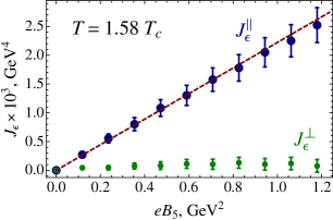
Figure 1: Energy flow (7) parallel ($J^{\|}_{\epsilon}$) and perpendicular ($J^{\perp}_{\epsilon}$) to the direction of the axial magnetic field $B_{5}$ in the deconfinement phase at $T=1.58\,T_{c}\equiv 479\,\mathrm{MeV}$. The red dashed line represents the best linear fit confirming the existence of the Axial Magnetic Effect (4). The slope of the fit is given by the conductivity (13).

In Fig. 1 we show the energy flow (7) as a function of the axial magnetic field $B_{5}$ in the deconfinement phase at $T=1.58\,T_{c}$. One can see that the energy flow parallel to the axial magnetic field $J^{\|}_{\epsilon}$ is a linear function of the field strength as predicted by the AME transport law (4). The energy flow in the transverse directions $J^{\perp}_{\epsilon}$ is zero within the error bars, as expected.

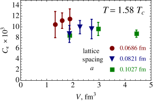
Figure 2: The dimensionless prefactor $C_{\epsilon}=J_{\epsilon}/(eB_{5}T^{2})$ as the function of the volume $V$ at three different values of the lattice spacing $a$. The expected theoretical value is $C_{\epsilon}=1/6$.

In Fig. 2 we demonstrate that our result does not depend (within reasonable error bars) on the volume of the system being simultaneously robust with respect to the variations of the lattice spacing (the latter plays a role of the inverse ultraviolet cutoff). To this end we have performed simulations on the lattices in the range $L_{s}=12\dots 18$ and $L_{t}=4\dots 8$ at $\beta=3.281,\ 3.398$ and $2.5$. We have also checked numerically that the usual magnetic field does not induce any energy flow.

The linear fit of the energy flow – shown by the dashed line in Fig. 1 – gives us the following value of the energy flow conductivity:

$$\sigma(T){\biggl{|}}_{T=1.58\,T_{c}}=2.22(3)\times 10^{-3}\,\mbox{GeV}^{2}\,.$$ (13)

For a conformal theory with two colors of fermions, the conductivity coefficient is expected to be $\sigma_{\mathrm{theor}}=T^{2}/6$ which gives us one order of magnitude larger value $\sigma_{\mathrm{theor}}\approx 0.0382\,\mathrm{GeV}^{2}$ at this temperature. We expect that this large difference is not related to the absence of the fermion vacuum loops in our simulations because the latter do not play an essential role in the AME Landsteiner:2011cp .

We see no signature of energy flow neither in the vicinity of the phase transition nor in the confinement phase.

Summarizing, we have numerically observed the existence of the Axial Magnetic Effect (AME) in the quenched $SU(2)$ gauge theory on the lattice. We have found that the equilibrium energy flow of massless fermions is parallel to the direction of (and proportional to the strength of) the time-independent uniform axial magnetic field. Our study also indirectly confirms the existence of the Chiral Vortical Effect (CVE) since both these effects have the same physical nature originating from the gravitational anomaly.

- (1) K. Fukushima, D. E. Kharzeev and H. J. Warringa, Phys. Rev. D 78, 074033 (2008); D. E. Kharzeev, L. D. McLerran and H. J. Warringa, Nucl. Phys. A 803, 227 (2008); A. Vilenkin, Phys. Rev. D 22, 3080 (1980); M. A. Metlitski and A. R. Zhitnitsky, Phys. Rev. D 72, 045011 (2005).
- (2) V. I. Zakharov, in Springer Lecture Notes in Physics ’Strongly Interacting Matter in Magnetic Fields’ edited by D. Kharzeev, K. Landsteiner, A. Schmitt, H.-U. Yee [arXiv:1210.2186 [hep-ph]].
- (3) B. I. Abelev et al. [STAR Collaboration], Phys. Rev. Lett. 103, 251601 (2009); Phys. Rev. C 81, 054908 (2010) [arXiv:0909.1717 [nucl-ex]]]; G. Wang [STAR Collaboration], arXiv:1210.5498 [nucl-ex]; S. A. Voloshin [STAR Collaboration], Indian J. Phys. 85, 1103 (2011); B. Abelev et al. [ALICE Collaboration], Phys. Rev. Lett. 110, 012301 (2013); Y. Hori [ALICE Collaboration], arXiv:1211.0890 [nucl-ex].
- (4) A. A. Zyuzin, Si Wu, A. A. Burkov, Phys. Rev. B 85, 165110 (2012); A. G. Grushin, Phys. Rev. D 86, 045001 (2012); A. A. Zyuzin, A. A. Burkov, Phys. Rev. B 86, 115133 (2012) [arXiv:1206.1868; P. Goswami, S. Tewari, arXiv:1210.6352 [cond-mat.mes-hall]; P. Goswami and B. Roy, arXiv:1211.4023 [cond-mat.mes-hall].
- (5) K. Landsteiner, E. Megias and F. Pena-Benitez, Phys. Rev. Lett. 107, 021601 (2011) and [arXiv:1207.5808].
- (6) J. Erdmenger, M. Haack, M. Kaminski and A. Yarom, JHEP 0901 (2009) 055; N. Banerjee, J. Bhattacharya, S. Bhattacharyya, S. Dutta, R. Loganayagam and P. Surowka, JHEP 1101 (2011) 094.
- (7) A. Vilenkin, Phys. Rev. D 20 (1979) 1807; A. Vilenkin, Phys. Rev. D 21 (1980) 2260.
- (8) K. Landsteiner, E. Megias, L. Melgar and F. Pena-Benitez, JHEP 1109 (2011) 121.
- (9) D. T. Son and P. Surowka, Phys. Rev. Lett. 103 (2009) 191601; Y. Neiman and Y. Oz, JHEP 1103 (2011) 023; A. V. Sadofyev, V. I. Shevchenko, and V. I. Zakharov, Phys. Rev. D 83, 105025 (2011); V. P. Nair, R. Ray and S. Roy, Phys. Rev. D 86, 025012 (2012).
- (10) K. Jensen, R. Loganayagam and A. Yarom, JHEP 1302 (2013) 088.
- (11) S. Golkar and D. T. Son, arXiv:1207.5806 [hep-th]; D. -F. Hou, H. Liu and H. -c. Ren, Phys. Rev. D 86 (2012) 121703.
- (12) P. V. Buividovich, M. N. Chernodub, E. V. Luschevskaya and M. I. Polikarpov, Phys. Rev. D 80, 054503 (2009); P. V. Buividovich et al., Phys. Rev. Lett. 105, 132001 (2010).
- (13) H. Neuberger, Phys. Lett. B 417, 141 (1998).
- (14) M. H. Al-Hashimi and U. J. Wiese, Annals Phys. 324, 343 (2009).
- (15) V. G. Bornyakov, E. M. Ilgenfritz, M. Muller-Preussker, Phys. Rev. D 72 (2005) 054511; V. G. Bornyakov, E. -M. Ilgenfritz, B. V. Martemyanov, S. M. Morozov, M. Muller-Preussker and A. I. Veselov, Phys. Rev. D 76, 054505 (2007).