Giant magneto-drag in graphene at charge neutrality

Abstract

We report experimental data and theoretical analysis of Coulomb drag between two closely positioned graphene monolayers in weak magnetic field. Close enough to the neutrality point, coexistence of electrons and holes in each layer leads to a dramatic increase of the drag resistivity. Away from charge neutrality, we observe non-zero Hall drag. The observed phenomena are explained by decoupling of electric and quasiparticle currents which are orthogonal at charge neutrality. The sign of magneto-drag depends on the energy relaxation rate and geometry of the sample.

Recent measurements Gorbachev12 of frictional drag in graphene-based double-layer devices revealed the unexpected phenomenon of giant magneto-drag at the charge neutrality point. Applying external magnetic fields as weak as 0.1-0.3 T results in the reversal of the sign and a dramatic enhancement of the amplitude of the drag resistance. If the device is doped away from charge neutrality, the impact of such a weak field on the drag resistance is very modest. The observed effect weakens at low temperatures, hinting at the classical origin of the phenomenon.

In this Letter we report experimental data on longitudinal and Hall drag resistivity in isolated graphene layers separated by a $1$ nm thick boron-nitride (hBN) spacer. The observed effects are explained in terms of coexisting electron and hole liquids in each layer Foster09 ; ryz . This theory is based on the hydrodynamic description of transport in graphene derived in Refs. Mueller08, ; Schuett13, ; lux, using the quantum kinetic equation framework Fritz08 ; Kashuba08 . It provides a simplified description of the magneto-drag effect while capturing the essentially classical physics of the phenomenon fn1 . The effect can be traced back to the fact that the Lorentz force in the electronic band is opposite to that in the hole band, which is also the reason for the anomalously large Nernst effect Zuev09 ; Wei09 and vanishing Hall effect at charge neutrality.

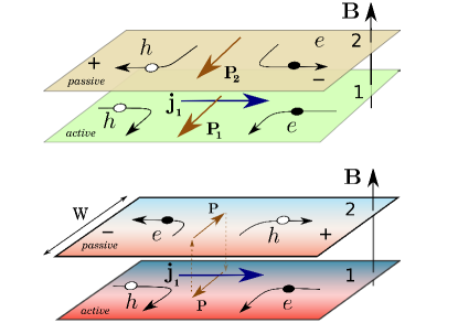
Figure 1: (Color online) Mechanism of magneto-drag at charge neutrality. Upper panel: in an infinite system quasi-particle currents in the two layers (denoted by ${\bm{P}}_{i}$) flow in the same direction, leading to positive drag $\rho^{D}_{xx}=V/j_{1}>0$. Lower panel: in a thermally isolated system no net quasi-particle flow is possible (leading to inhomogeneities in the quasi-particle density); the quasi-particle currents in the two layers have opposite directions yielding negative drag.

The classical mechanism behind the giant magneto-drag is illustrated in Fig. 1. The upper panel shows two infinite graphene layers at charge neutrality. The driving electric current $\bm{j}_{1}$ in the active layer corresponds to the the counter-propagating flow of electrons and holes with zero total momentum due to exact electron-hole symmetry (hence, in the absence of additional correlations there is no drag at the Dirac point Schuett13 ; DSarma07 ; Narozhny12 ; Polini12 ; Peres12 ). In a weak magnetic field, electrons and holes are deflected by the Lorentz force and drift in the same direction. The resulting quasi-particle flow, $\bm{P}_{1}$, carries a non-zero net momentum in the direction perpendicular to the charge flow, $\bm{j}_{1}$. The momentum transfer by the interlayer Coulomb interaction induces the quasi-particle current $\bm{P}_{2}$ in the same direction as $\bm{P}_{1}$. The Lorentz forces acting on both types of carriers in the passive layer drive the charge flow in the direction opposite to $\bm{j}_{1}$. If the passive circuit is open, this current is compensated by a finite drag voltage $V$, yielding a positive drag resistivity $\rho^{D}_{xx}=V/j_{1}>0$.

This mechanism of magneto-drag at charge neutrality is closely related to the anomalous Nernst effect in single-layer graphene Mueller08 ; Zuev09 ; Wei09 . Indeed, the quasi-particle current is proportional to the heat current at the Dirac point. A similar mechanism, where the role of $\bm{P}_{i}$ is played by a spin current, has been proposed in Ref. Abanin11 as a possible explanation for a giant non-local magnetoresistance at charge neutrality.

The above argument describes the steady state in the infinite system where all physical quantities are homogeneous in real space. This is not the case in a relatively small mesoscopic sample. Whether a particular sample should be considered “small” or “large” is determined by comparing the sample size to the typical length scale corresponding to the leading relaxation process. At high enough temperatures, the heat currents are most efficiently relaxed by electron-phonon scattering, which we describe in this Letter by the length scale $\ell_{\textrm{ph}}$ Levitov12 ; fn2 .

In a finite system, the quasi-particle currents must vanish at the boundaries. For $W\gg\ell_{\textrm{ph}}$, the quasi-particle current and density is homogeneous in the bulk and the system remains effectively infinite.

For $W\ll\ell_{\textrm{ph}}$, the currents $\bm{P}_{i}$ acquire a dependence on the coordinate $y$. In this case energy conservation dictates that $\bm{P}_{2}(y)=-\bm{P}_{1}(y)$. As the result the electric charge in the passive layer tends to flow in the same direction as $\bm{j}_{1}$, see Fig. 1. Thus, the drag is negative, which is the conventional sign for the Coulomb drag in a system with the same type of charge carriers.

In order to test the above ideas, we perform new measurements of the drag effect in magnetic field which are illustrated in Fig. 2. The experiments sup are carried out on graphene double-layer structure with 1 nm hBN spacer and two electrostatic gates. The schematics of the experiment is shown in the inset of the panel D in Fig. 2. The same device was used in Ref. Gorbachev12, for drag measurements in zero magnetic field.

The map for the drag resistivity, $\rho^{D}_{xx}(V_{T},V_{B})$, is shown in Fig. 2, panel A at $T=240$ K. The main difference compared to zero field experiment reported earlier Gorbachev12 is large negative drag at the double neutrality point. A dramatic change in drag resistivity with the applied magnetic field is shown in more details in Fig. 2, panels B and E (at $160$ K and $240$ K, respectively. To ensure same charge densities $n_{1}$ and $n_{2}$ in the top and bottom layers, we sweep both gates simultaneously along the line connecting the bottom left and top right corners of the map. The experiment shows a large negative drag resistivity close to the double neutrality point, $n_{1}=n_{2}=0$, as expected for a small sample (see above); in our device both layers have the width $W\approx 2\mu$m and sufficiently resistive contacts.

In addition to the longitudinal drag resistivity we also measure the Hall drag resistivity, $\rho^{D}_{xy}(V_{T},V_{B})$, shown in Fig. 2, panel C at $T=240$ K as a function of the top and bottom gate voltages. Due to the low density of states in graphene and the small separation between layers (in this experiment $d\approx 1$ nm), the relationship between gate voltages and charge densities is rather nontrivial. To identify sign of charge carriers at each point in Fig. 2, panel C, we also measured resistivity maps for both layers. Since the resistance of graphene is peaked at charge neutrality, tracking the position of the resistivity maximum gives the lines which divide the map into the electron- and hole-doped parts. Such lines are shown in both maps, see Fig. 2, panels C and A. The observed Hall drag resistance is large when one of the layers is close to neutrality point and vanishes if two layers have the same charge densities with opposite signs (a white line running from the top left to bottom right corner).

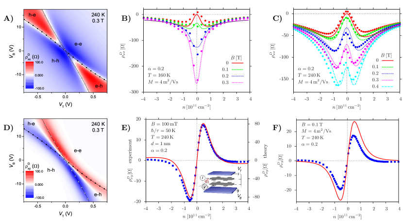
Figure 2: (Color online) Panel A: Longitudinal drag resistivity in magnetic field as a function of the top and bottom gate voltages. Lines track positions of the maxima in single-layer resistivity in top (open symbols) and bottom (closed symbols) layers. Panel B: Magneto-drag for equal charge densities $n_{1}=n_{2}=n$ at $T=160$ K. Solid symbols represent the experimental data. The lines show the results of the proposed theory (6), see Supplemental Material sup for details. Panel C: The map of Hall drag resistivity as function of top and bottom gate voltages. The white diagonal corresponds to vanishing Hall drag for $n_{1}=-n_{2}$. The lines are similar to those in the Panel A. Panel D: The experimental data (blue squares, left axis) and theoretical plot (red solid line, right axis) for the Hall drag resistivity for equal charge densities $n_{1}=n_{2}=n$. The theoretical curve is calculated on the basis of the microscopic theory of Ref. Schuett13, . Note the sign change at $n\approx\pm 2\times 10^{11}$cm^-2. Inset: schematics of Hall drag measurements in double layer system. The charge density is controlled by voltages $V_{T}$ and $V_{B}$ applied to the top and bottom gate, respectively. Panel E: Magneto-drag for equal charge densities $n_{1}=n_{2}=n$ at $T=240$ K. Solid symbols represent the experimental data. The lines show the results of the proposed theory (6). Panel F: The experimental data (blue squares) and the results of the proposed theory (6) (red solid line) for the Hall drag resistivity for equal charge densities $n_{1}=n_{2}=n$. The data are identical to those in Panel D.

We now turn to the theoretical description of the drag effect. Consider first the Drude model for electrons and holes in two layers,

$$e\bm{E}_{i}+e[\bm{v}_{ie}\times\bm{B}] = \bm{F}_{ie}+e\,\bm{v}_{ie}/M_{i},$$ (1a)

$$-e\bm{E}_{i}-e[\bm{v}_{ih}\times\bm{B}] = \bm{F}_{ih}+e\,\bm{v}_{ih}/M_{i},$$ (1b)

where $i=1,2$ and $\bm{v}_{ia}$, $a=e,h$, stand for the mean velocities of electrons and holes in the layer $i$, $\bm{E}_{1,2}$ and $\bm{B}$ are the electric and magnetic fields, $e$ is the elementary charge, and $M_{1,2}$ are the carrier mobilities due to scattering on impurities. The electric $\bm{j}_{i}$ and quasi-particle $\bm{P}_{i}$ currents are related to $\bm{v}_{ia}$ by Foster09

$$\bm{j}_{i}=e(n_{ie}\bm{v}_{ie}-n_{ih}\bm{v}_{ih}),\qquad\bm{P}_{i}=n_{ie}\bm{v}_{ie}+n_{ih}\bm{v}_{ih},$$ (2)

with $n_{ie(h)}=\int_{0}^{\infty}d\varepsilon\,\nu(\varepsilon)\left[e^{(\varepsilon\mp\mu_{i})/T}+1\right]^{-1}$ standing for the electron and hole densities. Here $\nu(\varepsilon)=2|\varepsilon|/\pi(\hbar v)^{2}$ is the density of states in graphene (disregarding the magnetic field), and $\mu_{i}$ are the chemical potentials measured from the Dirac point. The total charge and quasi-particle densities are defined as $n_{i}=n_{ie}-n_{ih}$ and $\rho_{i}=n_{ie}+n_{ih}$.

In general, the frictional force acting on each type of carriers can be represented by the sum

$$\bm{F}_{ia}=\hbar\sum\limits_{jb}\left[\gamma^{ab}_{ij}n_{jb}(\bm{v}_{ia}\!-\bm{v}_{jb})+\tilde{\gamma}^{ab}_{ij}n_{jb}(\bm{v}_{ia}\!+\bm{v}_{jb})\right],$$ (3)

where the coefficients $\tilde{\gamma}$ appear in monolayer graphene due to the absence of Gallilean invariance. The expression (3) can be obtained by solving the quantum kinetic equation (QKE) in the hydrodynamic approximation us2 . The dimensionless coefficients $\gamma^{ab}_{ij}$ and $\tilde{\gamma}^{ab}_{ij}$ are related to microscopic collision rates Schuett13 ; lux ; Mueller08 ; Fritz08 .

For $n_{i}=0$, the first term in Eq. (3) simplifies to

$$\bm{F}_{1a}=-\bm{F}_{2a}=\hbar\,\gamma\,(\bm{P}_{1}-\bm{P}_{2}),$$ (4)

where $\gamma=\hbar/T\tau_{P}$, with $\tau_{P}^{-1}$ being the momentum relaxation rate. The second term in Eq. (3) renormalizes the mobilities Schuett13 ; Fritz08 ; Kashuba08 . The Drude model (1) with the force (4) also describes the case $\mu_{1}=\mu_{2}\gg T$, where $\gamma=\hbar/\mu_{1}\tau_{P}$. In both limits, the model (1) is equivalent to the hydrodynamic transport equations derived from the QKE Schuett13 ; us2 .

For strongly-doped graphene, $\mu_{i}\gg T$, the quasi-particle current and density are obsolete: $\bm{P}_{i}=\bm{j}_{i}/e$ and $\rho_{i}=n_{i}$. Equations (1) are then reduced to the standard Drude model yielding the vanishing Hall drag resistivity $\rho_{xy}^{D}=E_{2y}/j_{1x}=0$ and conventional drag, $\rho^{D}_{xx}=E_{2x}/j_{1x}=-\hbar\gamma/e^{2}$, which show negligible dependence on the magnetic field Jauho93 .

In contrast, at charge neutrality the quasi-particle and charge degrees of freedom are decoupled. The quasi-particle density for $n_{i}=0$ is determined by the temperature as $\rho_{i}=\rho_{0}=\pi T^{2}/3(\hbar v)^{2}$, while the electric and quasi-particle currents $\bm{j}_{1}$ and $\bm{P}_{i}$ become orthogonal, as shown in Fig. 1.

Rewriting Eqs. (1), (4) in terms of currents and excluding $\bm{P}_{i}$, we obtain the resistivity tensor. At charge neutrality, $n_{i}=0$, the longitudinal drag resistivity is peaked and its value is given by the expression

$$\rho_{xx}^{D}=\frac{\hbar\,\gamma}{e^{2}}\,\frac{B^{2}M_{1}M_{2}}{1+\hbar\,\gamma\,\rho_{0}(M_{1}+M_{2})/e},\qquad n_{i}=0,$$ (5)

which describes positive drag in an infinite system in agreement with the qualitative picture illustrated in Fig. 1, upper panel. In the limit of weak interaction, $\gamma MT^{2}\ll\hbar ev^{2}$, the result (5) can be obtained from the standard perturbative approach Narozhny12 modified for graphene in a classical magnetic field.

Large negative peak in $\rho_{xx}^{D}$ at the double neutrality point (Fig. 2 panel B) suggests that the sample width, $W\approx 2\,\mu$m is relatively small as compared to $\ell_{\textrm{ph}}$ (Fig. 1, lower panel). To account for the finite sample width, we re-write the equations (1) in terms of the currents $\bm{j}_{i}$ and $\bm{P}_{i}$ and allow for the spatially varying quasi-particle density, $\rho_{i}$, in the sample. The resulting model for the first layer reads

$$-K_{1}\bm{\nabla}\rho_{1}+en_{1}\bm{E}_{1}+[\bm{j}_{1}\times\bm{B}] = \rho_{1}\bm{F}_{1}+e\bm{P}_{1}/M_{1},\mbox{\quad}$$ (6a)

$$e\rho_{1}\bm{E}_{1}+e[\bm{P}_{1}\times\bm{B}] = n_{1}\bm{F}_{1}+\bm{j}_{1}/M_{1},$$ (6b)

$$\bm{\nabla P}_{1}=-(\rho_{1}-\rho_{0})/\tau_{\textrm{ph}} - (\rho_{1}-\rho_{2})/(2\tau_{Q}).$$ (6c)

One has to replace the index $1$ with $2$ for the second layer. Here $K_{1}=(\pi\hbar^{2}v^{2}/2)\partial n_{1}/\partial\mu=2T\ln(2\cosh\mu_{1}/2T)$ is the mean quasi-particle kinetic energy. The continuity equation for the quasi-particle current (6c) includes relaxation by the electron-hole recombination Foster09 , with $\tau_{\textrm{ph}}^{-1}$ describing the energy loss from the system, which at high enough temperatures is dominated by phonon scattering fn2 , and $\tau_{Q}^{-1}$ describing the quasiparticle imbalance relaxation due to the interlayer Coulomb interaction. For $\tau_{\textrm{ph}}^{-1}=0$, one finds $\bm{P}_{1}+\bm{P}_{2}=0$ because the interlayer interaction does not lead to relaxation of the total quasiparticle current. Near the Dirac point, the energy and momentum relaxation rates coincide (in particular, $\tau_{Q}\sim\tau_{P}$). In doped graphene, the recombination rates are exponentially suppressed sup .

The continuity equation for the electric current simply reads $\bm{\nabla}\bm{j}_{i}=0$, hence $\bm{j}_{i}=(j_{i}(y),0)$. Within linear response, the density $\rho_{i}$ has to be substituted by the equilibrium value $\rho_{0}$ in the products $\rho_{i}\bm{F}$ and $\rho_{i}\bm{E}$. This way we obtain the linear system of differential equations on the functions $P_{iy}(y)$, $j_{1x}(y)$, and $\rho_{i}(y)$. Since the charge current acquires the dependence on the transverse coordinate, we define $\rho_{xx}^{D}=E_{2x}/\langle j_{1x}\rangle$, where $\langle j_{1x}\rangle=W^{-1}\int_{0}^{W}j_{1x}dy$.

The model (6) with the frictional force (4) admits a full analytic solution sup in terms of the relaxation rates $\tau_{Q}^{-1}$, $\tau_{\rm ph}^{-1}$, and $\tau_{P}^{-1}$. The resulting behavior crucially depends on these rates: in particular, in the absence of phonons ($\tau_{\rm ph}\rightarrow\infty$, i.e. in a thermally isolated system) the drag at the Dirac point is always negative, in agreement with the qualitative picture of Fig. 1. For vanishing sample width ($W\rightarrow 0$) we find $\rho_{xx}^{D}\approx-B^{2}W^{2}/(24\rho_{0}K\tau_{Q})$. In general, these rates depend on the carrier density and have to be determined by the microscopic theory Schuett13 . Relegating further mathematical details to the online Supplemental Material sup , we present the results of the model calculations in Fig. 2 alongside experimental data.

The drag resistivity $\rho_{xx}^{D}$ is plotted in Fig. 2, panels B and E for $T=160$ K and $T=240$ K, respectively. The collapse of the theoretical curves at high carrier density is an artifact of the phenomenological model fn2 , which is most reliable near charge neutrality. At higher temperature (Fig. 2, panel E), the drag resistivity exhibits qualitatively new features near charge neutrality which can be physically attributed to higher efficiency of relaxation processes. The sign of $\rho_{xx}^{D}$ at the Dirac point is then determined by the relation between the typical relaxation length $\ell_{\rm ph}=2\sqrt{K\tau_{\rm ph}M/e}$ and the sample width. This is illustrated in Fig. 3, where we plot $\rho_{xx}^{D}$ as a function of magnetic field for different values of the sample width choosing realistic values for the model parameters $T=240$ K, $M=4$ m${}^{2}/$Vs, and $\ell_{\textrm{ph}}=1.2\,\mu$m.

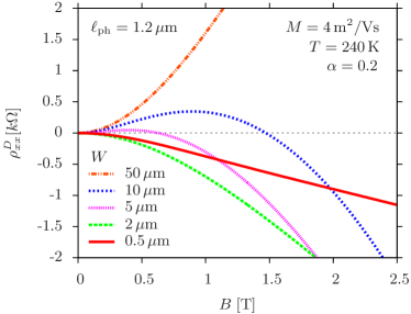
Figure 3: (Color online) The magnetic field dependence of the longitudinal drag resistivity at the neutrality point. The positive sign of the magneto-drag in weak fields corresponds to the limit $W\gg\ell_{\textrm{ph}}$, where $\ell_{\textrm{ph}}\approx 1.2\,\mu$m for the parameters of the plot. The magnetic field dependence of scattering rates is disregarded in the plot.

Based on the above results, we predict that in wider samples, the giant magneto-drag at the Dirac point should become positive. We also speculate that the magneto-drag at the double Dirac point may become positive in stronger fields due to the magnetic-field dependence of the scattering times $\tau_{\textrm{Q}}$, $\tau_{\textrm{P}}$, and $\tau_{\textrm{ph}}$.

The model (6) allows us to calculate the Hall drag resistivity $\rho_{xy}^{D}$. The result is shown in Fig. 2, panel F. The theory also predicts the vanishing Hall drag for the case of oppositely doped layers, $n_{1}=-n_{2}$. Interestingly enough, the data shows a sign change of $\rho_{xy}^{D}$ at $n\approx\pm 2\times 10^{11}$cm^-2. At that point the effect is rather weak and requires a more accurate consideration. Using the microscopic theory of Ref. Schuett13, , we have evaluated the Hall drag resistivity for an infinite sample with an energy-independent impurity scattering time $\tau$. The value of $\tau$ was determined from the single-layer resistivity measured in experiment and we have used the most plausible estimate for the value of the effective electron-electron interaction strength, $\alpha\approx 0.2$, in graphene on hBN. The result is shown in Fig. 2, panel D along with the corresponding experimental data without any fitting.

In conclusion, we have measured the longitudinal and Hall drag resistivity in double-layer graphene and provided a theoretical description of the observed effects. The giant magneto-drag at the neutrality point appears due to the presence of two types of carriers (electrons and holes), which in weak magnetic fields experience a unidirectional drift orthogonal to the driving current. This effect is specific to the neutrality point, where non-zero drag appears despite the exact electron-hole symmetry. The present theory does not rely on the Dirac spectrum in graphene, but is equivalent to the microscopic theory Schuett13 ; fn1 at and far away from the charge neutrality thus capturing the essential physics of magneto-drag. For a more accurate description of the effect at intermediate densities, the microscopic theory should be formulated on the basis of the kinetic equation us2 .

We are grateful to the Royal Society, the Körber Foundation, the Office of Naval Research, the Air Force Office of Scientific Research, the Engineering and Physical Sciences Research Council (UK), Stichting voor Fundamenteel Onderzoek der Materie (FOM, the Netherlands), DFG SPP 1459 and BMBF for support.

Upon completion of this manuscript, we became aware of a related work by Song and Levitov LevitovArXiv .

ONLINE SUPPORTING INFORMATION

I Experimental Devices and Measurement Procedures

The double layer graphene devices were fabricated by using procedures previously described in detail in Refs. Ponomarenko11, and Gorbachev12A, . The maximum size of our double-layer Hall bars is currently limited to, typically, 2 $\mu$m $\times$ 10 $\mu$m because of the formation of pockets of a hydrocarbon residue at the interface between graphene and BN (for details, see Supplementary Material in Ref. Ponomarenko11, ). These pockets (or bubbles) appear randomly, and our Hall bars are made to fit inside clean patches between bubbles. This restricts the width of double-layer devices to 1.5-2 $\mu$m. Making smaller and narrower Hall bars is impractical because of reduced mobility and difficulties associated with alignment of two Hall bars exactly on top of each other. Therefore, at present it is impossible to study magnetodrag in devices of different widths. The reported Hall bars had a width of 2 $\mu$m, and the overlapping area for top and bottom Hall bars was $\approx 15$ $\mu$m².

All experimental results presented in this work were obtained by using DC measurements with current commutation at each data point. We have chosen DC over AC measurements because in the latter case a significant out-of-phase signal (up to  30%) appears near the neutrality point even at frequencies as lows as $\sim$ 10-30 Hz. This signal originates probably from capacitance coupling between the closely spaced graphene layers. Each data point was measured for 12 seconds (6 sec for each polarity of the current), which corresponds to an effective frequency of 0.2 Hz, low enough to avoid the capacitive coupling. Further increase in the acquisition time improved accuracy but did not affect the reported curves.

To ensure that the measurements are done in the linear response regime, applied current was kept low. To this end, I-V curves were measured at representative points of the reported maps. . We have found empirically that a current of 50 nA can be used near the neutrality point where the nonlinearity is largest. At higher carrier densities, it is possible to increase the current by a factor of 10. The main reason for the nonlinearity is a voltage drop along the Hall bar. This voltage can be comparable to the difference between Fermi levels in the two graphene layers and, if the current is high, the voltage drop can result in a gradient of carrier concentration along the direction of current.

Furthermore, there is a finite tunnelling resistance through 3 atomic layers of BN separating top and bottom graphene Hall bars. At low biases used in all our measurements, the interlayer resistance $R_{T}$ exceeded 300 k$\Omega$ over the whole range of gate voltages. This value translates into a small contribution to the measured drag resistivity estimated as Halperin

$$\delta\rho_{xx}^{D}=\frac{L}{W}\frac{\rho^{2}}{12R_{T}}$$ (1)

for the case of equivalent layers. At the neutrality point at $T=240$ K we have $R_{T}=500$  k$\Omega$, $\rho=1$ k$\Omega$ is the intralayer resistivity (resistance per square) and the aspect ratio $L/W\approx 2$ for our sample. This yields the insignificant contribution $\delta\rho_{xx}^{D}\approx 0.33$ $\Omega$.

However, to ensure that the direct electrical coupling does not affect the measured drag resistance, we have also compared measurements with the passive graphene layer (the one where we measure drag voltage) being floated and grounded. In latter case, several different contacts were connected to the ground. If the tunnelling current is significant the grounded contacts should act as a sink and affect drag measurements. The difference was found insignificant for trilayer BN devices, as expected from the estimate (1). In contrast, devices with bilayer BN as a spacer exhibited very significant changes indicating that bilayers are too transparent to be used as an insulating layer for drag measurements.

Another important consideration in the reported measurements was to ensure that there was no additional AC current flowing through the devices due to external radiation at high frequencies, which could increase electron temperature in graphene with respect to cryostat temperature. To this end, radio frequency filters were fitted. Their efficiency was judged by the observation of strong suppression of a rectification signal (voltage in the absence of applied current), which could be comparable to drag voltage if no filters were used.

II Thickness of BN determined from transport measurements

The thickness of BN separating graphene layers was routinely determined during the device fabrication. To this end, we could use several techniques including atomic force microscopy (AFM) Dean10 , optical contrast Gorbachev11 ; Golla13 , Raman spectroscopy Gorbachev11 and tunnelling Britnell12 . In practice, the first two were found sufficient to determine the thickness with single-layer accuracy. The tunnelling resistance for the known device area was then used as an additional cross-check of the BN thickness. In this section we show that transport measurements provide yet another way to measure the thickness of the BN layer.

The approach is based on converting the Hall resistance measured in weak magnetic fields into carrier concentration and then finding the thickness as a fitting parameter from the gate voltage dependence of carrier concentration. In general the density is nonlinear complicated function of both gate voltages. However, if one of the layers is kept at the neutrality point, the density in the other layer acquires a relatively simple dependence on gate voltage. Our approach is similar to the one recently used by Kim et al. Kim12 .

Consider a 4-plate capacitor in Fig. 4, which consists of two grounded graphene sheets separated by a BN layer with thickness $d_{\textrm{int}}$ and two gates, top and bottom, isolated by relatively thick BN, with thicknesses $d_{T}$ and $d_{B}$, respectively. The charge densities in both graphene layers $n_{T}$ and $n_{B}$ are related to the applied gate voltages $V_{T}$ and $V_{B}$ through the system of nonlinear equations:

$$E_{T}\frac{d_{T}}{\varepsilon}+\frac{1}{e}E_{F}(n_{T})=V_{T},$$ (2)

$$E_{\textrm{int}}\frac{d_{\textrm{int}}}{\varepsilon}+\frac{1}{e}\left(E_{F}(n_{T})-E_{F}(n_{B})\right)=0,$$ (3)

$$E_{B}\frac{d_{B}}{\varepsilon}+\frac{1}{e}E_{F}(n_{B})=-V_{B},$$ (4)

$$E_{T}-E_{\textrm{int}}=\frac{en_{T}}{\varepsilon_{0}},$$ (5)

$$E_{\textrm{int}}-E_{B}=\frac{en_{B}}{\varepsilon_{0}},$$ (6)

where $E_{T}$, $E_{B}$ and $E_{\textrm{int}}$ are the electric fields in the top, bottom and middle BN layers, respectively, $\varepsilon=3.2$ is the dielectric constant of BN Kim12 , $\varepsilon_{0}$ the electric constant, $e$ the charge of electron and $E_{F}(n)=\operatorname{sign}(n)\hbar v_{F}\sqrt{\pi|n|}$ the Fermi energy in graphene ($v_{F}\approx 10^{6}$ m$/$s is the Fermi velocity; for simplicity we assume $T=0$ and no external doping). The Fermi energy is positive for electrons ($n>0$ ) and negative for holes ($n<0$). Eqs. (2-4) describe the potential drop across the top, middle and bottom BN, whereas Eqs. (5-6) follow from the Gauss law for the top and bottom graphene layers.

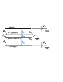
Figure 4: Sketch for 4-plate capacitor model.

If one of the graphene layers is at the neutrality point (e.g. for $n_{T}=0$), Eqs. (2-6) reduce to a one-line expression that links gate voltage directly to carrier density in the corresponding layer:

$$V_{B}=\frac{qd_{B}}{\varepsilon\varepsilon_{0}}n_{B}+\operatorname{sign}(n_{B})\frac{\hbar v_{F}\sqrt{\pi|n_{B}|}}{q}\left(1+\frac{d_{B}}{d_{\textrm{int}}}\right).$$ (7)

The first (linear) term gives the slope of $V_{B}(n_{B})$ at high densities and depends only on the thickness of the insulator separating graphene from the gate (this term is just the classical capacitance). The second (root-squared) term comes from the quantum capacitance of graphene and is responsible for nonlinear behaviour of the double-layer system close to the NP. The term depends on ratio $d_{B}/d_{\textrm{int}}$.

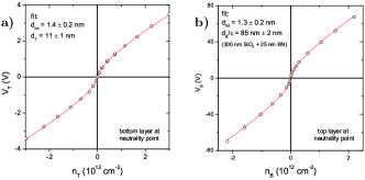
Figure 5: BN thickness extracted from transport measurements. (a) Density in the top graphene layer as a function of gate voltage applied to this layer, provided the bottom graphene layer is kept neutral. Open symbols – experiment; solid curve – best fit to Eq. (8). Different points correspond to different voltages applied to the bottom gate. (b) Same type of measurements as in (a) but with top and bottom layers interchanged. Both (a) and (b) give the same value of $d_{\textrm{int}}$.

Similar expression can be derived for $n_{B}=0$:

$$V_{T}=\frac{qd_{T}}{\varepsilon\varepsilon_{0}}n_{T}+\operatorname{sign}(n_{T})\frac{\hbar v_{F}\sqrt{\pi|n_{T}|}}{q}\left(1+\frac{d_{T}}{d_{\textrm{int}}}\right).$$ (8)

Therefore the thickness $d_{\textrm{int}}$ can be determined from two independent sets of measurements, presented in Figs. 5a and 5b. The experiment is carried out as the following. We fix $V_{B}$ and ramp $V_{T}$ recording Hall resistance for both layers. When the bottom layer reaches its neutrality point we record values of $V_{T}$ and $n_{T}$. This gives one data point in Fig. 5a. The same procedure is repeated for several $V_{B}$ until enough data are collected. Then the same procedure is carried out for fixed $V_{T}$, that is, the top and bottom layers are effectively swapped in these measurements. Within experimental accuracy, Figs. 5a and 5b yield the same value of $d_{\textrm{int}}$ which is $\approx 4$ times larger than interlayer spacing for bulk graphite and BN. This agrees well with the expected separation for the top and bottom graphene sheets if three BN layers are in between. This value is also in agreement with the AFM measurements carried on the same device.

III Phenomenological theory of double-layer devices

Here we present the full analytic solution of the theoretical model given by Eqs. (6) and (4) of the main text.

III.1 Model equations within linear response

Under the assumptions of linear response we have to re-write the equations (6) of the main text as follows [the frictional force is taken in the form (4) of the main text; for brevity we write equations for one layer only]

$$-\frac{\kappa_{1}}{en_{1}}\bm{\nabla}\rho_{1}+\bm{E}_{1}+R_{H}^{(1)}[\bm{j}_{1}\times\bm{e}_{z}]=e\frac{\rho_{0}}{n_{1}}\Gamma(\bm{P}_{1}-\bm{P}_{2})+eR_{0}^{(1)}\bm{P}_{1},$$ (9a)

$$\frac{\rho_{0}}{n_{1}}\bm{E}_{1}+eR_{H}^{(1)}[\bm{P}_{1}\times\bm{e}_{z}]=e\Gamma(\bm{P}_{1}-\bm{P}_{2})+R_{0}^{(1)}\bm{j}_{1}$$ (9b)

$$\bm{\nabla}\cdot\bm{P}_{1}=-\frac{\rho_{1}-\rho_{0}}{\tau_{\textrm{ph}}}-\frac{\rho_{1}-\rho_{2}}{2\tau_{\textrm{Q}}}.$$ (9c)

Here $R_{0}=1/(enM)$ and $R_{H}=B/(en)$ are the Drude and Hall resistances of the single-layer graphene far from the Dirac point; and $\Gamma=\gamma/e^{2}$ is the drag resistance far from the Dirac point and in zero field.

The above equations should be supplemented by the following boundary conditions: the quasiparticle currents must vanish at the edge of the sample

$$\bm{P}_{i}(y=0)=\bm{P}_{i}(y=W)=0,$$ (10a)

and on average no electric current is allowed in the passive layer

$$\overline{\bm{j}_{2}}=\frac{1}{W}\int\limits_{0}^{W}\!\!dy\,\bm{j}_{2}=0.$$ (10b)

The model (9) with the boundary conditions (10) admits a full analytic solution. The results simplify in the case of identical layers. The corresponding solutions are given below.

The results for inequivalent layers are qualitatively similar to the below solutions. We illustrate the dependence of magnetodrag in the double neutrality point on magnetic field in Fig. 6b for the case of different mobilities in the layers: $M=7$  m${}^{2}/Vs$ in the active layer and $M=3$  m${}^{2}/Vs$ and in the passive layer.

III.2 Drag between identical layers

Given the nonuniform current flow, the drag resistivity is defined as the ratio of the averaged induced voltage in the passive layer to the driving current in the active layer

$$\rho_{xx}^{D}=\frac{\overline{E_{2x}}}{\overline{j_{1x}}},$$ (11)

where the averaging was defined in Eq. (10b).

III.2.1 General expression

The resulting expression reads

$$\rho_{xx}^{D}=\frac{r_{0}}{2}\left[\frac{1}{1-\left[1-\frac{n^{2}}{\rho_{0}^{2}}\right]\frac{R_{H}^{2}}{R_{H}^{2}+R_{0}^{2}}\bar{f}_{+}}-\frac{1}{1-\frac{n^{2}}{\rho_{0}^{2}}\frac{2\Gamma}{2\Gamma+r_{0}}-\left[1-\frac{n^{2}}{\rho_{0}^{2}}\right]\frac{R_{H}^{2}}{R_{H}^{2}+R_{0}^{2}+\frac{\rho_{0}^{2}-n^{2}}{n^{2}}2\Gamma r_{0}}\bar{f}_{-}}\right],$$ (12)

where $r_{0}=1/(e\rho_{0}M)$ is the residual resistance of single-layer graphene at the Dirac point in the absence of magnetic field, and

$$\bar{f}_{\pm}=1-\frac{\tanh(W/L_{\pm})}{W/L_{\pm}},$$ (13)

with

$$L_{+}^{-2}=\frac{e^{2}n}{4\kappa\tau_{\rm ph}}R_{0}\left[1+\frac{R_{H}^{2}}{R_{0}^{2}}\right],\quad L_{-}^{-2}=\frac{e^{2}n}{4\kappa}R_{0}\left[\frac{1}{\tau_{\rm ph}}+\frac{1}{\tau_{Q}}\right]\left[\frac{2\Gamma}{r_{0}}\left(1-\frac{n^{2}}{\rho_{0}^{2}}\right)+1+\frac{R_{H}^{2}}{R_{0}^{2}}\right].$$ (14)

Note, that $R_{H}/R_{0}=BM$.

III.2.2 Drude limit

Far away from the Dirac point (i.e. for $\mu\gg T$) only one band contributes (such that $n=\rho_{0}$) and the result (12) simplifies to the standard Drude form which is independent of magnetic field

$$\rho_{xx}^{D}(\mu\gg T)=-\Gamma.$$ (15)

III.2.3 Zero field limit

In the absence of magnetic field $R_{H}=0$ and the result (12) simplifies to

$$\rho_{xx}^{D}(B=0)=\frac{r_{0}}{2}\left[1-\frac{1}{1-\frac{n^{2}}{\rho_{0}^{2}}\frac{2\Gamma}{2\Gamma+r_{0}}}\right].$$ (16)

Setting $n=\rho_{0}$ we recover the above Drude result. On the other hand at the Dirac point $n=0$ and drag vanishes

$$\rho_{xx}^{D}(B=0;n=0)=0.$$ (17)

III.2.4 Neutrality point

At the Dirac point ($n=0$) in the presence of magnetic field we find

$$\rho_{xx}^{D}(n=0)=\frac{r_{0}}{2}\left[\frac{1}{1-\bar{f}_{+}\frac{(BM)^{2}}{1+(BM)^{2}}}-\frac{1}{1-\bar{f}_{-}\frac{(BM)^{2}}{1+(BM)^{2}+2\Gamma/r_{0}}}\right].$$ (18)

Clearly, this result vanishes in the absence of the field.

III.2.5 Neutrality point in an infinite sample

Consider now the above result in the limit of an infinite sample $W\gg L_{+}$. (Note that $L_{+}>L_{-}$ by definition.) Then $\bar{f}_{\pm}=1$ and we find (in agreement with Eq. (5) of the main text)

$$\rho_{xx}^{D}(n=0;W\rightarrow\infty)=\frac{r_{0}}{2}\left[\frac{1}{1-\frac{(BM)^{2}}{1+(BM)^{2}}}-\frac{1}{1-\frac{(BM)^{2}}{1+(BM)^{2}+2\Gamma/r_{0}}}\right]=\frac{\Gamma r_{0}}{2\Gamma+r_{0}}(BM)^{2}>0.$$ (19)

The resulting drag is positive.

III.2.6 Neutrality point in a narrow sample

For completeness, let us now consider now a limit of a vanishing width $W\ll L_{-}$. Here $\bar{f}_{\pm}\approx W^{2}/(24L_{\pm}^{2})$ and expanding in this small factor we find

$$\rho_{xx}^{D}(n=0;W\rightarrow 0)\approx-r_{0}(BM)^{2}\frac{eW^{2}}{24M\kappa\tau_{Q}}<0.$$ (20)

The resulting drag is negative, independent of phonon scattering time and mobility (this can be seen by taking into account that the resistance $r_{0}$ is inversely proportional to the mobility).

III.3 Hall drag between identical layers

The Hall drag resistance is defined as

$$\rho_{xy}^{D}=\frac{\overline{E_{2y}}}{\overline{j_{1x}}},$$ (21)

where the averaging was defined in Eq. (10b).

The resulting expression for the Hall drag resistance is

$$\rho_{xy}^{D}=\frac{r_{0}}{2}\frac{n}{\rho_{0}}BM\left[\frac{1}{1-\left[1-\frac{n^{2}}{\rho_{0}^{2}}\right]\frac{R_{H}^{2}}{R_{H}^{2}+R_{0}^{2}}\bar{f}_{+}}-\frac{\frac{r_{0}}{2\Gamma+r_{0}}-\left(1-\frac{n^{2}}{\rho_{0}^{2}}\right)\frac{2\Gamma\bar{f}_{-}}{r_{0}\left[1+(BM)^{2}+\left(1-\frac{n^{2}}{\rho_{0}^{2}}\right)\frac{2\Gamma}{r_{0}}\right]}}{1-\frac{n^{2}}{\rho_{0}^{2}}\frac{2\Gamma}{2\Gamma+r_{0}}-\left[1-\frac{n^{2}}{\rho_{0}^{2}}\right]\frac{R_{H}^{2}}{R_{H}^{2}+R_{0}^{2}+\frac{\rho_{0}^{2}-n^{2}}{n^{2}}2\Gamma r_{0}}\bar{f}_{-}}\right],$$ (22)

where it is clear that Hall drag vanishes in the absence of the magnetic field and at the Dirac point as it should. It is also clear that Hall drag vanishes in the Drude limit where $n=\rho_{0}$.

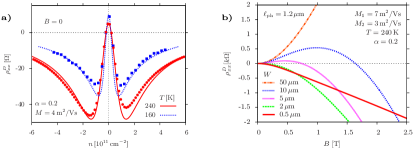
Figure 6: Left Panel: Fit of the zero-field drag resistivity. This fit is used to determine the phenomenological friction coefficient $\gamma$. Note, that the theoretical curve in this plot is shifted vertically to fit the shape of the experimental data. The obtained $\gamma$ is subsequently used to calculate magnetodrag. Right Panel: magneto-drag at charge neutrality calculated for different sample widths in the case of inequivalent layers.

IV Relaxation rates

In order to determine how the above results depend on carrier density, we need to estimate the dependence of the scattering rates $\tau_{Q}^{-1}$, $\tau_{\rm ph}^{-1}$ and the phenomenological coefficient $\gamma$ on the chemical potential and temperature. While comparing our theory to the experimental data, we use the interpolation formulas listed below, such that the only remaining fitting parameters are the electron-electron and electron-phonon coupling constants ($\alpha$ and $g_{\rm ph}$, respectively).

IV.1 Momentum relaxation rate

Since the drag at zero magnetic field is entirely determined by the ”friction coefficient” $\gamma$ we can use earlier theoretical work Narozhny12A ; Schuett13A and actual experimental data to fit $\gamma$. The result is a function of a single parameter that has the following general properties: (i) $\gamma\propto\alpha^{2}$, (ii) $\gamma\rightarrow 0$ for $\mu\gg T$, and (iii) $\gamma$ remains finite at the Dirac point.

For $T=240\,$K, the system can be approximately regarded as ballistic. In this case, microscopic calculations show that at the Dirac point $\gamma(\mu=0)\sim\alpha^{2}$, while far away from the Dirac point $\gamma(\mu\gg T)\sim\alpha^{2}T^{2}/\mu^{2}$. In the intermediate region $\mu\sim T$ the momentum relaxation rate is given by a complicated integral, but effectively it just interpolates between the two limits. Given that the phenomenological theory is only accurate in those two limits, we may use a simple interpolation

$$\gamma=\frac{\alpha^{2}}{1+\mu^{2}/2T^{2}}.$$ (23)

For $T=160$ K, the system enters the diffusive regime which complicates the theory. We use our earlier estimates of the drag resistance in the diffusive regime Narozhny12A and fit the dimensionless relaxation rate $\gamma$ to the drag data at zero magnetic field, see Fig. 6. Within the phenomenological theory, the zero-field drag resistance is given by Eq. (16). Using this result and respecting the above general restrictions on $\gamma$ we arrive at the empirical expression, which is applicable for not too high values of the chemical potential:

$$\gamma\approx\frac{\alpha^{2}}{\sqrt{4+(\mu/T)^{2}(1+0.35\ln^{2}(\mu/T))}}.$$ (24)

IV.2 Energy relaxation rate

The lowest order phonon contribution to the electron-hole recombination in graphene is kinematically forbidden (within the same valley). There are, however, many possible mechanisms of recombination Foster09A ; Song12 , all of them involving phonons. Therefore, we phenomenologically regard the time and length scale of electron and hole recombination as $\tau_{\textrm{ph}}$ and $\ell_{\textrm{ph}}$.

The microscopic theory Schuett13A includes thermoelectric effects formulated in terms of energy currents. In graphene the energy current is equal to the total momentum Schuett13A . Therefore, the corresponding relaxation processes do not require recombination and can be directly attributed to phonons.

The quasiparticle relaxation rate due to the scattering on phonons can be estimated with the help of the Fermi golden rule. The result is

$$\frac{1}{\tau_{\rm ph}}=\frac{g_{\rm ph}^{2}(T)T}{\cosh(\mu/T)}.$$ (25)

This estimate includes the disorder-assisted electron-phonon scattering processes Song12 as well as phonon-induced intervalley scattering and is valid for temperatures below the Debye temperature in hBN.

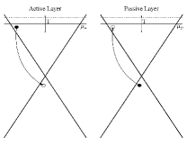
Figure 7: Sketch of the quasi-particle relaxation between two layers

IV.3 Imbalance relaxation

The quasiparticle recombination rate due to the energy transfer between the graphene layers can also be estimated by means of the Fermi Golden Rule in the two limits $\mu\ll T$ and $\mu\gg T$. Interpolating between the two limits, we obtain the following estimate

$$\frac{1}{\tau_{Q}}=\frac{\alpha^{2}\sqrt{T^{2}+\mu^{2}}}{4\cosh(\mu/T)}.$$ (26)

The corresponding process is illustrated in Fig. 7.

References

- (1) R. V. Gorbachev, A. K. Geim, M. I. Katsnelson, K. S. Novoselov, T. Tudorovskiy, I. V. Grigorieva, A. H. MacDonald, K. Watanabe, T. Taniguchi, L. A. Ponomarenko, Nature Phys. 8, 896 (2012).
- (2) M. S. Foster and I. L. Aleiner, Phys. Rev. B 79, 085415 (2009).
- (3) D. Svintsov, V. Vyurkov, S. Yurchenko, T. Otsuji, and V. Ryzhii, J. Appl. Phys. 111, 083715 (2012).
- (4) M. Müller and S. Sachdev, Phys. Rev. B 78, 115419 (2008); M. Müller, L. Fritz, and S. Sachdev, ibid, 115406 (2008).
- (5) M. Schütt, P. M. Ostrovsky, M. Titov, I. V. Gornyi, B. N. Narozhny, and A. D. Mirlin, Phys. Rev. Lett. 110, 026601 (2013); M. Schütt, PhD thesis (Karlsruhe Institute of Technology) http://digbib.ubka.uni-karlsruhe.de/volltexte/1000036515 (2013).
- (6) J. Lux and L. Fritz, Phys. Rev. B 86, 165446 (2012).
- (7) L. Fritz, J. Schmalian, M. Mueller, and S. Sachdev, Phys. Rev. B 78, 085416 (2008); M. Müller, J. Schmalian, and L. Fritz, Phys. Rev. Lett. 103, 025301 (2009).
- (8) A. B. Kashuba, Phys. Rev. B 78, 085415 (2008).
- (9) The hydrodynamic description of drag in graphene derived in Ref. Schuett13, was justified by the singular behavior of the collision integral due to kinematics of Dirac fermions. This singularity leads to the fast unidirectional thermalization and allows one to select the relevant eigenmodes of the collision integral Fritz08 ; Mueller08 . Projecting the collision integral onto these modes, one arrives at the effective model in terms of energy and electric currents, which is equivalent to Eq. (1) with the generalized force (4). At the Dirac point the energy current is equivalent to the quasi-particle current .
- (10) Y. M. Zuev, W. Chang, and P. Kim, Phys. Rev. Lett. 102, 096807 (2009).
- (11) P. Wei, W. Z. Bao, Y. Pu, C. N. Lau, and J. Shi, Phys. Rev. Lett. 102, 166808 (2009).
- (12) W. Tse, B. Yu-K. Hu, and S. Das Sarma, Phys. Rev. B 76, 081401 (2007).
- (13) B. N. Narozhny, M. Titov, I. V. Gornyi, and P. M. Ostrovsky, Phys. Rev. B 85, 195421 (2012).
- (14) M. Carrega, T. Tudorovskiy, A. Principi, M. I. Katsnelson, and M. Polini, New J. Phys. 14, 063033 (2012).
- (15) B. Amorim and N. M. R. Peres, J. Phys.: Cond. Mat. 24, 335602 (2012).
- (16) D. A. Abanin, S. V. Morozov, L. A. Ponomarenko, R. V. Gorbachev, A. S. Mayorov, M. I. Katsnelson, K. Watanabe, T. Taniguchi, K. S. Novoselov, L. S. Levitov, and A. K. Geim, Science 332, 328 (2011).
- (17) The lowest order phonon contribution to the electron-hole recombination in graphene is kinematically forbidden. There are, however, many possible mechanisms of recombination Foster09 ; Levitov12 , all of them involving phonons. Therefore, we phenomenologically regard the time and length scale of electron and hole recombination as and . Moreover, the microscopic theory Schuett13 ; us2 includes thermoelectric effects formulated in terms of energy currents rather. In graphene the energy current is equal to the total momentum Schuett13 . Therefore, the corresponding relaxation processes do not require recombination and can be directly attributed to phonons. At the same time, the hydrodynamic description in terms of the energy currents yields only the power-law decay of the magneto-drag at , in contrast to the exponential collapse shown in Fig. 2, panels B and E.
- (18) J. C. W. Song, M. Y. Reizer, and L. S. Levitov, Phys. Rev. Lett. 109, 106602 (2012).
- (19) See Appendix for details.
- (20) M. Schütt et al., in preparation.
- (21) A.-P. Jauho and H. Smith, Phys. Rev. B, 47 4420 (1993); K. Flensberg, B. Y. Hu, A.-P. Jauho, J. M. Kinaret, Phys. Rev. B 52, 14761 (1995); A. Kamenev and Y. Oreg, Phys. Rev. B 52, 7516 (1995).
- (22) J. C. W. Song and L. S. Levitov, arXiv:1303.3529 (2013).

References

- (1) L. A. Ponomarenko et al., Nature Phys. 7, 958 (2011).
- (2) R. V. Gorbachev et al., Nature Physics 8, 896 (2012).
- (3) Y. Oreg and B. I. Halperin Phys. Rev. B 60, 5679 (1999).
- (4) C. Dean et al., Nature Nanotech 5, 722 (2010).
- (5) R. V. Gorbachev et al., SMALL 7, 465 (2011).
- (6) D. Golla et al., Appl. Phys. Lett., 102, 161906 (2013).
- (7) L. Britnell et al., Nano Letters 12, 1707 (2012).
- (8) S. Kim et al., Phys. Rev. Lett. 108, 116404 (2012).
- (9) B. N. Narozhny, M. Titov, I. V. Gornyi, and P. M. Ostrovsky, Phys. Rev. B 85, 195421 (2012).
- (10) M. Schütt, P. M. Ostrovsky, M. Titov, I. V. Gornyi, B. N. Narozhny, and A. D. Mirlin, Phys. Rev. Lett. 110, 026601 (2013); M. Schütt, PhD thesis (2013).
- (11) J. C. W. Song, M. Y. Reizer, and L. S. Levitov, Phys. Rev. Lett. 109, 106602 (2012).
- (12) M. S. Foster and I. L. Aleiner, Phys. Rev. B 79, 085415 (2009).