Integral representations of the weighted geometric mean and the logarithmic mean

Abstract.

In the paper, the authors show that the weighted geometric mean and the logarithmic mean are Bernstein functions and establish integral representations of these means by Cauchy’s integral theorem in the theory of complex functions.

1. Introduction

1.1. Some definitions

We recall some notions and definitions.

Definition 1.1 ([12, 24]).

A function $f$ is said to be completely monotonic on an interval $I$ if $f$ has derivatives of all orders on $I$ and

$$(-1)^{n}f^{(n)}(t)\geq 0$$ (1.1)

for $x\in I$ and $n\geq 0$.

Definition 1.2 ([1]).

If $f^{(k)}(t)$ for some nonnegative integer $k$ is completely monotonic on an interval $I$, but $f^{(k-1)}(t)$ is not completely monotonic on $I$, then $f(t)$ is called a completely monotonic function of $k$-th order on an interval $I$.

Definition 1.3 ([15, 17]).

A function $f$ is said to be logarithmically completely monotonic on an interval $I$ if its logarithm $\ln f$ satisfies

$$(-1)^{k}[\ln f(t)]^{(k)}\geq 0$$ (1.2)

for $k\in\mathbb{N}$ on $I$.

Definition 1.4 ([22, 24]).

A function $f:I\subseteq(-\infty,\infty)\to[0,\infty)$ is called a Bernstein function on $I$ if $f(t)$ has derivatives of all orders and $f^{\prime}(t)$ is completely monotonic on $I$.

Definition 1.5 ([22, p. 19, Definition 2.1]).

A Stieltjes function is a function $f:(0,\infty)\to[0,\infty)$ which can be written in the form

$$f(x)=\frac{a}{x}+b+\int_{0}^{\infty}\frac{1}{s+x}{\operatorname{d\mspace{-2.0mu}}\mu(s)},$$ (1.3)

where $a,b\geq 0$ are nonnegative constants and $\mu$ is a nonnegative measure on $(0,\infty)$ such that

$$\int_{0}^{\infty}\frac{1}{1+s}\operatorname{d\mspace{-2.0mu}}\mu(s)<\infty.$$

In the newly-published paper [7], a new notion “completely monotonic degree” of functions on $(0,\infty)$ was naturally introduced and initially studied.

It has been proved in [2, 8, 15, 17] that a logarithmically completely monotonic function on an interval $I$ must be completely monotonic on $I$. The set of logarithmically completely monotonic functions on $(0,\infty)$ contains all Stieltjes functions, see [2] or [19, Remark 4.8].

It is obvious that any nonnegative completely monotonic function of first order is a Bernstein function.

Bernstein functions can be characterized by [22, p. 15, Theorem 3.2] which states that a function $f:(0,\infty)\to\mathbb{R}$ is a Bernstein function if and only if it admits the representation

$$f(x)=a+bx+\int_{0}^{\infty}\bigl{(}1-e^{-xt}\bigr{)}\operatorname{d\mspace{-2.0mu}}\mu(t),$$ (1.4)

where $a,b\geq 0$ and $\mu$ is a measure on $(0,\infty)$ satisfying

$$\int_{0}^{\infty}\min\{1,t\}\operatorname{d\mspace{-2.0mu}}\mu(t)<\infty.$$

The relation between Bernstein functions and logarithmically completely monotonic functions was discovered in [5, pp. 161–162, Theorem 3] and [22, p. 45, Proposition 5.17], which reads that the reciprocal of any Bernstein function is logarithmically completely monotonic.

1.2. Some means

We also recall that the extended mean value $E(r,s;x,y)$ may be defined as

$$E(r,s;x,y) =\biggl{[}\frac{r(y^{s}-x^{s})}{s(y^{r}-x^{r})}\biggr{]}^{{1/(s-r)}}, rs(r-s)(x-y) \neq 0;$$ (1.5)

$$E(r,0;x,y) =\biggl{[}\frac{y^{r}-x^{r}}{r(\ln y-\ln x)}\biggr{]}^{{1/r}}, r(x-y) \neq 0;$$ (1.6)

$$E(r,r;x,y) =\frac{1}{e^{1/r}}\biggl{(}\frac{x^{x^{r}}}{y^{y^{r}}}\biggr{)}^{{1/(x^{r}-y^{r})}}, r(x-y) \neq 0;$$ (1.7)

$$E(0,0;x,y) =\sqrt{xy}\,, x \neq y;$$ (1.8)

$$E(r,s;x,x) =x, x =y;$$

where $x$ and $y$ are positive numbers and $r,s\in\mathbb{R}$. Because this mean was first defined in [23], so it is also called Stolarsky’s mean. Many special means with two positive variables are special cases of $E$, for example,

$$E(r,2r;x,y) =M_{r}(x,y), (\text{power mean})$$

$$E(1,p;x,y) =L_{p}(x,y), (\text{generalized logarithmic mean})$$

$$E(1,1;x,y) =I(x,y), (\text{exponential mean})$$

$$E(1,2;x,y) =A(x,y), (\text{arithmetic mean})$$

$$E(0,0;x,y) =G(x,y), (\text{geometric mean})$$

$$E(-2,-1;x,y) =H(x,y), (\text{harmonic mean})$$

$$E(0,1;x,y) =L(x,y). (\text{logarithmic mean})$$

For more information on $E$, please refer to the monograph [4], the papers [9, 10, 11], and a lot of closely-related references therein.

1.3. The arithmetic mean is a Bernstein function

It is easy to see that the arithmetic mean

$$A_{x,y}(t)=A(x+t,y+t)=A(x,y)+t$$

is a trivial Bernstein function of $t\in(-\min\{x,y\},\infty)$ for $x,y>0$.

1.4. The harmonic mean is a Bernstein function

In [21], the harmonic mean

$$H_{x,y}(t)=H(x+t,y+t)=\frac{2}{\frac{1}{x+t}+\frac{1}{y+t}}$$ (1.9)

for $t\in(-\min\{x,y\},\infty)$ and $x,y>0$ with $x\neq y$ was proved to be a Bernstein function and

$$H_{x,y}(s)=H(x,y)+s+\frac{(x-y)^{2}}{4}\int_{0}^{\infty}\bigl{(}1-e^{-su}\bigr{)}e^{-(x+y)u/2}\operatorname{d\mspace{-2.0mu}}u,$$ (1.10)

$$H(x,y)=A(x,y)-\frac{(x-y)^{2}}{2}\int_{0}^{\infty}e^{-(x+y)u}\operatorname{d\mspace{-2.0mu}}u,$$ (1.11)

$$H(s,y+s)=s+\frac{y^{2}}{4}\int_{0}^{\infty}\bigl{(}1-e^{-su}\bigr{)}e^{-yu/2}\operatorname{d\mspace{-2.0mu}}u.$$ (1.12)

1.5. The exponential mean is a Bernstein function

In [18, p. 116, Remark 6], it was pointed out that the reciprocal of the exponential mean

$$I_{x,y}(t)=I(x+t,y+t)=\frac{1}{e}\biggl{[}\frac{(x+t)^{x+t}}{(y+t)^{y+t}}\biggr{]}^{{1/(x-y)}}$$ (1.13)

for $x,y>0$ with $x\neq y$ is a logarithmically completely monotonic function of $t\in(-\min\{x,y\},\infty)$ and that, by using

$$I(x,y)=\exp\biggl{(}\frac{1}{y-x}\int_{x}^{y}\ln u\operatorname{d\mspace{-2.0mu}}u\biggr{)},$$ (1.14)

the exponential mean $I_{x,y}(t)$ for $t>-\min\{x,y\}$ with $x\neq y$ is also a completely monotonic function of first order (that is, a Bernstein function).

1.6. The logarithmic mean is a Bernstein function

In [13, p. 616], it was concluded that the logarithmic mean

$$L_{x,y}(t)=L(x+t,y+t)$$ (1.15)

is increasing and concave in $t>-\min\{x,y\}$ for $x,y>0$ with $x\neq y$. More strongly, it was proved in [16, Theorem 1] that the logarithmic mean $L_{x,y}(t)$ for $x,y>0$ with $x\neq y$ is a completely monotonic function of first order in $t\in(-\min\{x,y\},\infty)$, that is, the logarithmic mean $L_{x,y}(t)$ is a Bernstein function of $t\in(-\min\{x,y\},\infty)$. The proof of [16, Theorem 1] is based on making use of the integral representation

$$L(x,y)=\int_{0}^{1}x^{u}y^{1-u}\operatorname{d\mspace{-2.0mu}}u$$ (1.16)

and proving that the weighted geometric mean

$$G_{x,y;\lambda}(t)=(x+t)^{\lambda}(y+t)^{1-\lambda}$$ (1.17)

for $\lambda\in(0,1)$ and $x,y\in\mathbb{R}$ with $x\neq y$ is a Bernstein function of $t>-\min\{x,y\}$.

1.7. The geometric mean is a Bernstein function

After the weighted geometric mean $G_{x,y;\lambda}(t)$ was proved in [16] to be a Bernstein function, the statement that the geometric mean $G_{x,y;1/2}(t)$ is a Bernstein function was recently recovered in [21] by several approaches. More importantly, the integral representation

$$G_{x,y;1/2}(z)=G(x,y)+z+\frac{(x-y)^{2}}{2\pi}\int_{0}^{\infty}\frac{\rho((x-y)s)}{s}e^{-ys}\bigl{(}1-e^{-sz}\bigr{)}\operatorname{d\mspace{-2.0mu}}s$$ (1.18)

for $x>y>0$ and $z\in\mathbb{C}\setminus(-\infty,-y]$ was established in [21], where

$$\rho(s) =\int_{0}^{1/2}q(u)\bigl{[}1-e^{-(1-2u)s}\bigr{]}e^{-us}\operatorname{d\mspace{-2.0mu}}u$$ (1.19)

$$=\int_{0}^{1/2}q\biggl{(}\frac{1}{2}-u\biggr{)}\bigl{(}e^{us}-e^{-us}\bigr{)}e^{-s/2}\operatorname{d\mspace{-2.0mu}}u$$

$$\geq 0$$

on $(0,\infty)$ and

$$q(u)=\sqrt{\frac{1}{u}-1}\,-\frac{1}{\sqrt{1/u-1}\,}$$ (1.20)

on $(0,1)$.

Let $0<a_{k}\leq a_{k+1}$ for $1\leq k\leq n-1$ and $a+z=(a_{1}+z,a_{2}+z,\dotsc,a_{n}+z)$ for $z\in\mathbb{C}\setminus(-\infty,-a_{1}]$. Then the geometric mean

$$G_{n}(a+z)=\sqrt[n]{\prod_{\ell=1}^{n}(a_{\ell}+z)}$$

has the integral representation

$$G_{n}(a+z)=A_{n}(a)+z-\frac{1}{\pi}\sum_{\ell=1}^{n-1}\sin\frac{\ell\pi}{n}\int_{a_{\ell}}^{a_{\ell+1}}\Biggl{|}\prod_{k=1}^{n}(a_{k}-t)\Biggr{|}^{1/n}\frac{\operatorname{d\mspace{-2.0mu}}t}{t+z}.$$ (1.21)

This conclusion was gained in [20]. From this, it is easy to see that the geometric mean $G_{n}(a+t)$ is a Bernstein function of $t\in(-a_{1},\infty)$. More interestingly, the well-known inequality between $A_{n}(a)$ and $G_{n}(a)$ can be derived from (1.21).

1.8. Main results of this paper

In this paper, we will find an integral representation of the weighted geometric mean $G_{x,y;\lambda}(t)$ defined by (1.17), and then substitute it into (1.16) to obtain a new integral representation of the logarithmic mean.

2. Lemmas

For proving our main results, we need the following lemmas.

Lemma 2.1.

For $t>0$ and $\alpha\in(-1,1)$, let

$$h_{\alpha}(t)=\biggl{(}1+\frac{1}{t}\biggr{)}^{\alpha}.$$ (2.1)

Then the derivatives of $h_{\alpha}(t)$ can be computed by

$$h_{\alpha}^{(m)}(t)=\frac{(-1)^{m}}{t^{m}(1+t)^{m}}\biggl{(}1+\frac{1}{t}\biggr{)}^{\alpha}\sum_{k=0}^{m-1}{a_{\alpha,m,k}t^{k}},$$ (2.2)

where $m\in\mathbb{N}$ and

$$a_{\alpha,m,k}=k!\binom{m}{k}\binom{m-1}{k}\prod_{\ell=0}^{m-k-1}(\alpha+\ell).$$ (2.3)

Consequently,

1. if $\alpha\in(0,1)$, the function $h_{\alpha}(t)$ is completely monotonic on $(0,\infty)$;

2. if $\alpha\in(-1,0)$, the function $h_{\alpha}(t)$ is a Bernstein function on $(0,\infty)$;

3. the derivatives of the function

   $$H_{\alpha}(t)=\frac{h_{\alpha}(t)}{\alpha}-\frac{h_{\alpha-1}(t)}{\alpha-1}$$ (2.4)

   may be calculated by

   $$H_{\alpha}^{(m)}(t)=\frac{(-1)^{m}}{t^{m}(1+t)^{m+1}}\biggl{(}1+\frac{1}{t}\biggr{)}^{\alpha}\sum_{k=0}^{m-1}{b_{\alpha,m,k}t^{k}},$$ (2.5)

   where $m\in\mathbb{N}$ and

   $$b_{\alpha,m,k}=k!\binom{m+1}{k}\binom{m-1}{k}\prod_{\ell=1}^{m-k-1}(\alpha+\ell);$$ (2.6)

4. the function $H_{\alpha}(t)$ is completely monotonic for all $\alpha\in(0,1)$ on $(0,\infty)$.

Proof.

It is easy to see that

$$h_{\alpha}^{\prime}(t)=-\alpha\biggl{(}1+\frac{1}{t}\biggr{)}^{\alpha-1}\frac{1}{t^{2}}=-\alpha\biggl{(}1+\frac{1}{t}\biggr{)}^{\alpha}\frac{1}{t(1+t)}.$$

This means that the formulas (2.2) and (2.3) are valid for $m=1$.

Assume that the formulas (2.2) and (2.3) are valid for some $m>1$. By this inductive hypothesis, a simple calculation gives

$$h_{\alpha}^{(m+1)}(t)=\bigl{[}h_{\alpha}^{(m)}(t)\bigr{]}^{\prime}=\Biggl{[}\frac{(-1)^{m}}{t^{m}(1+t)^{m}}\biggl{(}1+\frac{1}{t}\biggr{)}^{\alpha}\sum_{k=0}^{m-1}{a_{\alpha,m,k}t^{k}}\Biggr{]}^{\prime}\\ \begin{aligned} &=(-1)^{m+1}\sum_{k=0}^{m-1}\frac{a_{\alpha,m,k}}{[t^{m+\alpha-k}(1+t)^{m-\alpha}]^{2}}\\ &\quad\times\bigl{[}(m+\alpha-k)t^{m+\alpha-k-1}(1+t)^{m-\alpha}+(m-\alpha)t^{m+\alpha-k}(1+t)^{m-\alpha-1}\bigr{]}\\ &=\frac{(-1)^{m+1}}{t^{m+1}(1+t)^{m+1}}\biggl{(}1+\frac{1}{t}\biggr{)}^{\alpha}\sum_{k=0}^{m-1}a_{\alpha,m,k}[m+\alpha-k+(2m-k)t]t^{k}\\ &=\frac{(-1)^{m+1}}{t^{m+1}(1+t)^{m+1}}\biggl{(}1+\frac{1}{t}\biggr{)}^{\alpha}\Biggl{\{}(m+\alpha)a_{\alpha,m,0}+(m+1)a_{\alpha,m,m-1}t^{m}\\ &\quad+\sum_{k=1}^{m-1}[(m+\alpha-k){a_{\alpha,m,k}}+(2m-k+1){a_{\alpha,m,k-1}}]t^{k}\Biggr{\}}\\ &=\frac{(-1)^{m+1}}{t^{m+1}(1+t)^{m+1}}\biggl{(}1+\frac{1}{t}\biggr{)}^{\alpha}\sum_{k=0}^{m}{a_{\alpha,m+1,k}t^{k}}.\end{aligned}$$

This shows that the formulas (2.2) and (2.3) are valid for all $m\geq 1$.

The left proofs are straightforward, so we omit them. The proof of Lemma 2.1 is completed. ∎

Lemma 2.2.

For $\alpha\in(-1,1)$ and $z\in\mathbb{C}\setminus(-\infty,0]$, the principal branch of the function $h_{\alpha}(z)$ has the integral representation

$$h_{\alpha}(z)=1+\frac{\sin(\alpha\pi)}{\pi}\int_{0}^{1}\biggl{(}\frac{1}{u}-1\biggr{)}^{\alpha}\frac{\operatorname{d\mspace{-2.0mu}}u}{u+z}.$$ (2.7)

Consequently, the function $h_{\alpha}(t)$ is a Stieltjes function for $\alpha\in(0,1)$ and a Bernstein function for $\alpha\in(-1,0)$ on $(0,\infty)$.

Proof.

By standard arguments, we can obtain immediately that

$$\lim_{z\to 0}[zh_{\alpha}(z)]=\lim_{z\to 0}\biggl{[}z\biggl{(}1+\frac{1}{z}\biggr{)}^{\alpha}\biggr{]}=\lim_{z\to 0}\bigl{[}z^{1-\alpha}(1+z)^{\alpha}\bigr{]}=0,$$ (2.8)

$$\lim_{z\to\infty}h_{\alpha}(z)=\lim_{z\to\infty}\biggl{(}1+\frac{1}{z}\biggr{)}^{\alpha}=1,$$ (2.9)

and

$$h_{\alpha}(\overline{z})=\overline{h_{\alpha}(z)}.$$ (2.10)

For $t\in(0,\infty)$ and $\varepsilon>0$, we have

$$h_{\alpha}(-t+i\varepsilon) =\biggl{(}1+\frac{1}{-t+i\varepsilon}\biggr{)}^{\alpha}$$

$$=\biggl{(}\frac{1-t+i\varepsilon}{-t+i\varepsilon}\biggr{)}^{\alpha}$$

$$=\biggl{[}\frac{(1-t+i\varepsilon)(-t-i\varepsilon)}{t^{2}+\varepsilon^{2}}\biggr{]}^{\alpha}$$

$$=\biggl{(}\frac{t^{2}-t+\varepsilon^{2}-i\varepsilon}{t^{2}+\varepsilon^{2}}\biggr{)}^{\alpha}$$

$$=\exp\biggl{[}\alpha\biggl{(}\ln\left|\frac{t^{2}-t+\varepsilon^{2}-i\varepsilon}{t^{2}+\varepsilon^{2}}\right|+i\arg\frac{t^{2}-t+\varepsilon^{2}-i\varepsilon}{t^{2}+\varepsilon^{2}}\biggr{)}\biggr{]}$$

$$=\begin{cases}\exp\biggl{[}\alpha\biggl{(}\ln\left|\dfrac{t^{2}-t+\varepsilon^{2}-i\varepsilon}{t^{2}+\varepsilon^{2}}\right|&\\ \hskip 20.00003pt-i\arctan\dfrac{\varepsilon}{t^{2}-t+\varepsilon^{2}}\biggr{)}\biggr{]},&t^{2}-t+\varepsilon^{2}>0\\ \exp\biggl{[}\alpha\biggl{(}\ln\left|\dfrac{t^{2}-t+\varepsilon^{2}-i\varepsilon}{t^{2}+\varepsilon^{2}}\right|&\\ \hskip 20.00003pt+i\arctan\dfrac{\varepsilon}{t^{2}-t+\varepsilon^{2}}-\pi i\biggr{)}\biggr{]},&t^{2}-t+\varepsilon^{2}<0\\ \exp\biggl{[}\alpha\biggl{(}\ln\dfrac{\varepsilon}{t^{2}+\varepsilon^{2}}-\dfrac{\pi i}{2}\biggr{)}\biggr{]},&t^{2}-t+\varepsilon^{2}=0\end{cases}$$

$$\to\begin{cases}\exp\biggl{(}\alpha\ln\dfrac{t-1}{t}\biggr{)},&t>1\\ \exp\biggl{[}\alpha\biggl{(}\ln\dfrac{1-t}{t}-\pi i\biggr{)}\biggr{]},&0<t<1\\ 0,&t=1\end{cases}$$

$$=\begin{cases}\biggl{(}\dfrac{t-1}{t}\biggr{)}^{\alpha},&t>1\\ \biggl{(}\dfrac{1-t}{t}\biggr{)}^{\alpha}[\cos(\alpha\pi)-\sin(\alpha\pi)],&0<t<1\\ 0,&t=1\end{cases}$$

as $\varepsilon\to 0^{+}$. As a result,

$$\lim_{\varepsilon\to 0^{+}}\Im f(-t+i\varepsilon)=\begin{cases}0,&t\geq 1;\\ -\biggl{(}\dfrac{1}{t}-1\biggr{)}^{\alpha}\sin(\alpha\pi),&0<t<1.\end{cases}$$ (2.11)

Let $D$ be a bounded domain with piecewise smooth boundary $\partial D$. The famous Cauchy integral formula (see [6, p. 113]) reads that if $f(z)$ is holomorphic on $D$ and if $f(z)$ extends smoothly to the boundary $\partial D$ of $D$, then

$$f(z)=\frac{1}{2\pi i}\oint_{\partial D}\frac{f(w)}{w-z}\operatorname{d\mspace{-2.0mu}}w,\quad z\in D.$$ (2.12)

For any but fixed point $z\in\mathbb{C}\setminus(-\infty,0]$, choose $0<\varepsilon<1$ and $r>0$ such that $0<\varepsilon<|z|<r$, and consider the positively oriented contour $C(\varepsilon,r)$ in $\mathbb{C}\setminus(-\infty,0]$ consisting of the half circle $z=\varepsilon e^{i\theta}$ for $\theta\in\bigl{[}-\frac{\pi}{2},\frac{\pi}{2}\bigr{]}$ and the half lines $z=x\pm i\varepsilon$ for $x\leq 0$ until they cut the circle $|z|=r$, which close the contour at the points $-r(\varepsilon)\pm i\varepsilon$, where $0<r(\varepsilon)\to r$ as $\varepsilon\to 0$. See Figure 1.

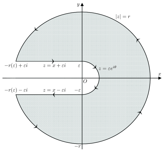
Figure 1. The contour $C(\varepsilon,r)$

By the above mentioned Cauchy integral formula, we have

$$\begin{split}h_{\alpha}(z)&=\frac{1}{2\pi i}\oint_{C(\varepsilon,r)}\frac{h_{\alpha}(w)}{w-z}\operatorname{d\mspace{-2.0mu}}w\\ &=\frac{1}{2\pi i}\biggl{[}\int_{\pi/2}^{-\pi/2}\frac{i\varepsilon e^{i\theta}h\bigl{(}\varepsilon e^{i\theta}\bigr{)}}{\varepsilon e^{i\theta}-z}\operatorname{d\mspace{-2.0mu}}\theta+\int_{-r(\varepsilon)}^{0}\frac{h_{\alpha}(x+i\varepsilon)}{x+i\varepsilon-z}\operatorname{d\mspace{-2.0mu}}x\\ &\quad+\int_{0}^{-r(\varepsilon)}\frac{h_{\alpha}(x-i\varepsilon)}{x-i\varepsilon-z}\operatorname{d\mspace{-2.0mu}}x+\int_{\arg[-r(\varepsilon)-i\varepsilon]}^{\arg[-r(\varepsilon)+i\varepsilon]}\frac{ire^{i\theta}h\bigl{(}re^{i\theta}\bigr{)}}{re^{i\theta}-z}\operatorname{d\mspace{-2.0mu}}\theta\biggr{]}.\end{split}$$ (2.13)

By the limit (2.8), it follows that

$$\lim_{\varepsilon\to 0^{+}}\int_{\pi/2}^{-\pi/2}\frac{i\varepsilon e^{i\theta}h_{\alpha}\bigl{(}\varepsilon e^{i\theta}\bigr{)}}{\varepsilon e^{i\theta}-z}\operatorname{d\mspace{-2.0mu}}\theta=0.$$ (2.14)

In virtue of the limit (2.9), we can derive that

$$\lim_{\begin{subarray}{c}\varepsilon\to 0^{+}\\ r\to\infty\end{subarray}}\int_{\arg[-r(\varepsilon)-i\varepsilon]}^{\arg[-r(\varepsilon)+i\varepsilon]}\frac{ire^{i\theta}h_{\alpha}\bigl{(}re^{i\theta}\bigr{)}}{re^{i\theta}-z}\operatorname{d\mspace{-2.0mu}}\theta=\lim_{r\to\infty}\int_{-\pi}^{\pi}\frac{ire^{i\theta}h_{\alpha}\bigl{(}re^{i\theta}\bigr{)}}{re^{i\theta}-z}\operatorname{d\mspace{-2.0mu}}\theta=2\pi i.$$ (2.15)

Making use of the limits (2.10) and (2.11) leads to

$$\quad\int_{-r(\varepsilon)}^{0}\frac{h_{\alpha}(x+i\varepsilon)}{x+i\varepsilon-z}\operatorname{d\mspace{-2.0mu}}x+\int_{0}^{-r(\varepsilon)}\frac{h_{\alpha}(x-i\varepsilon)}{x-i\varepsilon-z}\operatorname{d\mspace{-2.0mu}}x$$

$$=\int_{-r(\varepsilon)}^{0}\biggl{[}\frac{h_{\alpha}(x+i\varepsilon)}{x+i\varepsilon-z}-\frac{h_{\alpha}(x-i\varepsilon)}{x-i\varepsilon-z}\biggr{]}\operatorname{d\mspace{-2.0mu}}x$$

$$=\int_{-r(\varepsilon)}^{0}\frac{(x-i\varepsilon-z)h_{\alpha}(x+i\varepsilon)-(x+i\varepsilon-z)h_{\alpha}(x-i\varepsilon)}{(x+i\varepsilon-z)(x-i\varepsilon-z)}\operatorname{d\mspace{-2.0mu}}x$$

$$=\int_{-r(\varepsilon)}^{0}\frac{(x-z)[h_{\alpha}(x+i\varepsilon)-h_{\alpha}(x-i\varepsilon)]-i\varepsilon[h_{\alpha}(x-i\varepsilon)+h_{\alpha}(x+i\varepsilon)]}{(x+i\varepsilon-z)(x-i\varepsilon-z)}\operatorname{d\mspace{-2.0mu}}x$$

$$=2i\int_{-r(\varepsilon)}^{0}\frac{(x-z)\Im h_{\alpha}(x+i\varepsilon)-\varepsilon\Re h_{\alpha}(x+i\varepsilon)}{(x+i\varepsilon-z)(x-i\varepsilon-z)}\operatorname{d\mspace{-2.0mu}}x$$

$$\to 2i\int_{-r}^{0}\frac{\lim_{\varepsilon\to 0^{+}}\Im h_{\alpha}(x+i\varepsilon)}{x-z}\operatorname{d\mspace{-2.0mu}}x$$

$$=-2i\int^{r}_{0}\frac{\lim_{\varepsilon\to 0^{+}}\Im h_{\alpha}(-t+i\varepsilon)}{t+z}\operatorname{d\mspace{-2.0mu}}t$$

$$\to-2i\int^{\infty}_{0}\frac{\lim_{\varepsilon\to 0^{+}}\Im h_{\alpha}(-t+i\varepsilon)}{t+z}\operatorname{d\mspace{-2.0mu}}t$$

$$=2i\sin(\alpha\pi)\int_{0}^{1}\biggl{(}\frac{1}{t}-1\biggr{)}^{\alpha}\frac{\operatorname{d\mspace{-2.0mu}}t}{t+z}$$ (2.16)

as $\varepsilon\to 0^{+}$ and $r\to\infty$. Substituting equations (2.14), (2.15), and (2.16) into (2.13) and simplifying produce the integral representation (2.7). The proof of Lemma 2.2 is completed. ∎

3. An integral representation of the weighted geometric mean

Utilizing lemmas in the above section, we now prove that the weighted geometric mean $G_{x,y;\lambda}(t)$ is a Bernstein function of $t>-\min\{x,y\}$ and present an integral representation of the geometric mean $G_{x,y;\lambda}(z)$ for $z\in\mathbb{C}\setminus(-\infty,-\min\{x,y\}]$.

Theorem 3.1.

For $\lambda\in(0,1)$ and $x,y\in\mathbb{R}$ with $x\neq y$, the weighted geometric mean $G_{x,y;\lambda}(t)$ defined by (1.17) is a Bernstein function of $t>-\min\{x,y\}$.

Proof.

When $x>y>0$, a direct differentiation yields

$$G_{x,y;\lambda}^{\prime}(t) =\lambda(1-\lambda)\biggl{[}\frac{1}{\lambda}\biggl{(}\frac{x+t}{y+t}\biggr{)}^{\lambda}+\frac{1}{1-\lambda}\biggl{(}\frac{y+t}{x+t}\biggr{)}^{1-\lambda}\biggr{]}$$

$$=\lambda(1-\lambda)\biggl{[}\frac{1}{\lambda}\biggl{(}1+\frac{x-y}{y+t}\biggr{)}^{\lambda}-\frac{1}{\lambda-1}\biggl{(}1+\frac{x-y}{y+t}\biggr{)}^{\lambda-1}\biggr{]}$$

$$=\lambda(1-\lambda)\biggl{[}\frac{1}{\lambda}h_{\lambda}\biggl{(}\frac{y+t}{x-y}\biggr{)}-\frac{1}{\lambda-1}h_{\lambda-1}\biggl{(}\frac{y+t}{x-y}\biggr{)}\biggr{]}$$

$$=\lambda(1-\lambda)H_{\lambda}\biggl{(}\frac{y+t}{x-y}\biggr{)}.$$ (3.1)

By the complete monotonicity of the function $H_{\alpha}$ obtained in Lemma 2.1, it is immediate to see that the derivative $G_{x,y;\lambda}^{\prime}(t)$ is completely monotonic, and so the geometric mean $G_{x,y;\lambda}(t)$ is a Bernstein function for $x>y>0$ and $\lambda\in(0,1)$. Considering the symmetry property

$$G_{x,y;\lambda}(t)=G_{y,x;1-\lambda}(t)$$ (3.2)

reveals that, no matter $y>x>0$ or $x>y>0$, the geometric mean $G_{x,y;\lambda}(t)$ is a Bernstein function of $t>-\min\{x,y\}$. ∎

Theorem 3.2.

For $\lambda\in(0,1)$ and $x>y>0$, the principal branch of the weighted geometric mean $G_{x,y;\lambda}(z)$ defined by (1.17) has the integral representation

$$G_{x,y;\lambda}(z)=x^{\lambda}y^{1-\lambda}+z\\ +\frac{\sin(\lambda\pi)}{\pi}(x-y)\int_{0}^{\infty}\frac{F(\lambda,(x-y)s)}{s}e^{-sy}(1-e^{-sz})\operatorname{d\mspace{-2.0mu}}s,$$ (3.3)

where $z\in\mathbb{C}\setminus(-\infty,-y]$ and

$$F(\lambda,s)=\int_{0}^{1}\biggl{(}\frac{1}{u}-1\biggr{)}^{\lambda}\biggl{(}1-\frac{\lambda}{1-u}\biggr{)}e^{-us}\operatorname{d\mspace{-2.0mu}}u>0.$$ (3.4)

Consequently, the geometric mean $G_{x,y;\lambda}(t)$ for $\lambda\in(0,1)$ and $x,y>0$ is a Bernstein function of $t>-\min\{x,y\}$.

Proof.

By the integral representation (2.7) in Lemma 2.2, we have

$$H_{\lambda}\biggl{(}\frac{y+z}{x-y}\biggr{)}=\frac{1}{\lambda(1-\lambda)}+\int_{0}^{1}Q_{\lambda}(u)\frac{\operatorname{d\mspace{-2.0mu}}u}{u+\frac{y+z}{x-y}},$$

where $H_{\lambda}$ is defined by (3.1) and

$$Q_{\lambda}(u) =\frac{\sin(\lambda\pi)}{\lambda\pi}\biggl{(}\frac{1}{u}-1\biggr{)}^{\lambda}-\frac{\sin[(\lambda-1)\pi]}{(\lambda-1)\pi}\biggl{(}\frac{1}{u}-1\biggr{)}^{\lambda-1}$$

$$=\frac{\sin(\lambda\pi)}{\pi}\biggl{(}\frac{1}{u}-1\biggr{)}^{\lambda}\biggl{[}\frac{1}{\lambda}-\frac{1}{1-\lambda}\biggl{(}\frac{1}{u}-1\biggr{)}^{-1}\biggr{]}$$

$$=\frac{\sin(\lambda\pi)}{\lambda(1-\lambda)\pi}\biggl{(}\frac{1}{u}-1\biggr{)}^{\lambda}\biggl{(}1-\frac{\lambda}{1-u}\biggr{)}.$$

Accordingly,

$$G_{x,y;\lambda}^{\prime}(z) =1+\lambda(1-\lambda)\int_{0}^{1}Q_{\lambda}(u)\frac{\operatorname{d\mspace{-2.0mu}}u}{u+\frac{y+z}{x-y}}$$

$$=1+\frac{\sin(\lambda\pi)}{\pi}\int_{0}^{\infty}F(\lambda,s)\exp\biggl{(}-\frac{y+z}{x-y}s\biggr{)}\operatorname{d\mspace{-2.0mu}}s.$$

Integrating on both sides of this equation with respect to $z$ from $0$ to $w$ gives

$$G_{x,y;\lambda}(w) =G_{x,y;\lambda}(0)+w$$

$$\quad+\frac{\sin(\lambda\pi)}{\pi}\int_{0}^{\infty}F(\lambda,s)\biggl{[}\int_{0}^{w}\exp\biggl{(}-\frac{y+z}{x-y}s\biggr{)}\operatorname{d\mspace{-2.0mu}}z\biggr{]}\operatorname{d\mspace{-2.0mu}}s$$

$$=x^{\lambda}y^{1-\lambda}+w+\frac{\sin(\lambda\pi)}{\pi}(x-y)$$

$$\quad\times\int_{0}^{\infty}\frac{F(\lambda,s)}{s}\exp\biggl{(}-\frac{sy}{x-y}\biggr{)}\biggl{[}1-\exp\biggl{(}-\frac{sw}{x-y}\biggr{)}\biggr{]}\operatorname{d\mspace{-2.0mu}}s.$$

Changing the variable $s$ by $(x-y)s$ and replacing $w$ by $z$ in the above integral lead to the integral representation (3.3).

It is obvious that

$$F(\lambda,s) =\biggl{(}\int_{0}^{1-\lambda}+\int_{1-\lambda}^{1}\biggr{)}\biggl{(}\frac{1}{u}-1\biggr{)}^{\lambda}\biggl{(}1-\frac{\lambda}{1-u}\biggr{)}e^{-us}\operatorname{d\mspace{-2.0mu}}u$$

$$>e^{-(1-\lambda)s}\biggl{(}\int_{0}^{1-\lambda}+\int_{1-\lambda}^{1}\biggr{)}\biggl{(}\frac{1}{u}-1\biggr{)}^{\lambda}\biggl{(}1-\frac{\lambda}{1-u}\biggr{)}\operatorname{d\mspace{-2.0mu}}u$$

$$=e^{-(1-\lambda)s}\int_{0}^{1}\biggl{(}\frac{1}{u}-1\biggr{)}^{\lambda}\biggl{(}1-\frac{\lambda}{1-u}\biggr{)}\operatorname{d\mspace{-2.0mu}}u$$

$$=0.$$

The proof of Theorem 3.2 is completed. ∎

Corollary 3.1.

For $\lambda\in(0,1)$ and $x>y>0$, the difference between the weighted arithmetic and geometric means has the following integral representation

$$\bigl{[}\lambda x+(1-\lambda)y\bigr{]}-x^{\lambda}y^{1-\lambda}=\frac{\sin(\lambda\pi)}{\pi}(x-y)\int_{0}^{\infty}\frac{F(\lambda,(x-y)s)}{s}e^{-sy}\operatorname{d\mspace{-2.0mu}}s,$$ (3.5)

where $F(\lambda,s)$ is defined by (3.4). Consequently, the weighted arithmetic mean of two positive numbers is not less than the weighted geometric mean of two positive numbers.

Proof.

This follows from taking $z\to\infty$ on both sides of (3.3) and making use of the fact that

$$\lim_{z\to\infty}[G_{x,y;\lambda}(z)-z] =\lim_{z\to\infty}\biggl{\{}z\biggl{[}\biggl{(}1+\frac{x}{z}\biggr{)}^{\lambda}\biggl{(}1+\frac{y}{z}\biggr{)}^{1-\lambda}-1\biggr{]}\biggr{\}}$$

$$=\lim_{z\to 0}\frac{(1+{x}z)^{\lambda}(1+{y}z)^{1-\lambda}-1}{z}$$

$$=\lambda x+(1-\lambda)y.$$

Corollary 3.1 is thus proved. ∎

4. An integral representation of the logarithmic mean

Employing the integral representation (3.3) in Theorem 3.2, we now derive an integral representation of the logarithmic mean $L_{x,y}(z)$ for $z\in\mathbb{C}\setminus(-\infty,-\min\{x,y\}]$.

Theorem 4.1.

For $x>y>0$, the logarithmic mean $L_{x,y}(z)$ defined by (1.15) has the integral representation

$$L_{x,y}(z)=L(x,y)+z+\frac{x-y}{\pi}\int_{0}^{\infty}\frac{P_{x,y}(s)}{s}e^{-sy}\bigl{(}1-e^{-sz}\bigr{)}\operatorname{d\mspace{-2.0mu}}s$$ (4.1)

for $z\in\mathbb{C}\setminus(-\infty,-y]$, where

$$P_{x,y}(s)=\int_{0}^{1}\sin(\lambda\pi)F(\lambda,(x-y)s)\operatorname{d\mspace{-2.0mu}}\lambda$$ (4.2)

and the function $F$ is defined by (3.4). Consequently, the logarithmic mean $L_{x,y}(t)$ is a Bernstein function of $t>-\min\{x,y\}$.

Proof.

This may be deduced from integrating with respect to $\lambda$ from $0$ to $1$ on both sides of (3.3) and considering (1.16). ∎

Corollary 4.1.

For $x>y>0$, the difference between the arithmetic and logarithmic means satisfies

$$A(x,y)-L(x,y)=\frac{x-y}{\pi}\int_{0}^{\infty}\frac{P_{x,y}(s)}{s}e^{-sy}\operatorname{d\mspace{-2.0mu}}s,$$ (4.3)

where the function $P_{x,y}(s)$ is defined by (4.2).

Proof.

This may be derived from letting $z\to\infty$ on both sides of (4.1) and using the fact that $\lim_{z\to\infty}[L_{x,y}(z)-z]=A(x,y)$. Corollary 4.1 is thus proved. ∎

Remark 4.1.

The multi-variable analogy of the integral representation (3.3) has been established in [20] and has been employed in [14] to find an integral representation of Stirling numbers of the first kind. Some results in this paper were included in the thesis [25].

Remark 4.2.

After this paper was completed, we found the paper [3] which is motivated by the paper [16] and discovered some conditions on $r$ and $s$ such that Stolarsky’s $E(r,s;x+t,y+t)$ are Bernstein functions of $t$.

References

- [1] R. D. Atanassov and U. V. Tsoukrovski, Some properties of a class of logarithmically completely monotonic functions, C. R. Acad. Bulgare Sci. 41 (1988), no. 2, 21–23.
- [2] C. Berg, Integral representation of some functions related to the gamma function, Mediterr. J. Math. 1 (2004), no. 4, 433–439; Available online at http://dx.doi.org/10.1007/s00009-004-0022-6.
- [3] Á. Besenyei, On comoplete monotonicity of some functions related to means, Math. Inequal. Appl. 16 (2013), no. 1, 233–239; Available online at http://dx.doi.org/10.7153/mia-16-17.
- [4] P. S. Bullen, Handbook of Means and Their Inequalities, Mathematics and its Applications, Volume 560, Kluwer Academic Publishers, Dordrecht-Boston-London, 2003.
- [5] C.-P. Chen, F. Qi, and H. M. Srivastava, Some properties of functions related to the gamma and psi functions, Integral Transforms Spec. Funct. 21 (2010), no. 2, 153–164; Available online at http://dx.doi.org/10.1080/10652460903064216.
- [6] T. W. Gamelin, Complex Analysis, Undergraduate Texts in Mathematics, Springer, New York-Berlin-Heidelberg, 2001.
- [7] B.-N. Guo and F. Qi, A completely monotonic function involving the tri-gamma function and with degree one, Appl. Math. Comput. 218 (2012), no. 19, 9890–9897; Available online at http://dx.doi.org/10.1016/j.amc.2012.03.075.
- [8] B.-N. Guo and F. Qi, A property of logarithmically absolutely monotonic functions and the logarithmically complete monotonicity of a power-exponential function, Politehn. Univ. Bucharest Sci. Bull. Ser. A Appl. Math. Phys. 72 (2010), no. 2, 21–30.
- [9] B.-N. Guo and F. Qi, A simple proof of logarithmic convexity of extended mean values, Numer. Algorithms 52 (2009), no. 1, 89–92; Available online at http://dx.doi.org/10.1007/s11075-008-9259-7.
- [10] B.-N. Guo and F. Qi, The function : Logarithmic convexity and applications to extended mean values, Filomat 25 (2011), no. 4, 63–73; Available online at http://dx.doi.org/10.2298/FIL1104063G.
- [11] B.-N. Guo and F. Qi, The function : Ratio’s properties, available online at http://arxiv.org/abs/0904.1115.
- [12] D. S. Mitrinović, J. E. Pečarić, and A. M. Fink, Classical and New Inequalities in Analysis, Kluwer Academic Publishers, 1993.
- [13] F. Qi, A new lower bound in the second Kershaw’s double inequality, J. Comput. Appl. Math. 214 (2008), no. 2, 610–616; Availbale online at http://dx.doi.org/10.1016/j.cam.2007.03.016.
- [14] F. Qi, Integral representations and properties of Stirling numbers of the first kind, J. Number Theory 133 (2013), no. 7, 2307–2319; Available online at http://dx.doi.org/10.1016/j.jnt.2012.12.015.
- [15] F. Qi and C.-P. Chen, A complete monotonicity property of the gamma function, J. Math. Anal. Appl. 296 (2004), no. 2, 603–607; Available online at http://dx.doi.org/10.1016/j.jmaa.2004.04.026.
- [16] F. Qi and S.-X. Chen, Complete monotonicity of the logarithmic mean, Math. Inequal. Appl. 10 (2007), no. 4, 799–804; Available online at http://dx.doi.org/10.7153/mia-10-73.
- [17] F. Qi and B.-N. Guo, Complete monotonicities of functions involving the gamma and digamma functions, RGMIA Res. Rep. Coll. 7 (2004), no. 1, Art. 8, 63–72; Available online at http://rgmia.org/v7n1.php.
- [18] F. Qi, S. Guo, and S.-X. Chen, A new upper bound in the second Kershaw’s double inequality and its generalizations, J. Comput. Appl. Math. 220 (2008), no. 1-2, 111–118; Available online at http://dx.doi.org/10.1016/j.cam.2007.07.037.
- [19] F. Qi, C.-F. Wei, and B.-N. Guo, Complete monotonicity of a function involving the ratio of gamma functions and applications, Banach J. Math. Anal. 6 (2012), no. 1, 35–44.
- [20] F. Qi, X.-J. Zhang, and W.-H. Li, A new proof of the geometric-arithmetic mean inequality by Cauchy’s integral formula, available online at http://arxiv.org/abs/1301.6432.
- [21] F. Qi, X.-J. Zhang, and W.-H. Li, Some Bernstein functions and integral representations concerning harmonic and geometric means, available online at http://arxiv.org/abs/1301.6430.
- [22] R. L. Schilling, R. Song, and Z. Vondraček, Bernstein Functions, de Gruyter Studies in Mathematics 37, De Gruyter, Berlin, Germany, 2010.
- [23] K. B. Stolarsky, Generalizations of the logarithmic mean, Math. Mag. 48 (1975), 87–92.
- [24] D. V. Widder, The Laplace Transform, Princeton University Press, Princeton, 1946.
- [25] X.-J. Zhang, Integral Representations, Properties, and Applications of Three Classes of Functions, Thesis supervised by Professor Feng Qi and submitted for the Master Degree of Science at Tianjin Polytechnic University in January 2013. (Chinese)