Towards Automatic Model Comparison:
An Adaptive Sequential Monte Carlo Approach

Abstract

Model comparison for the purposes of selection, averaging and validation is a problem found throughout statistics. Within the Bayesian paradigm, these problems all require the calculation of the posterior probabilities of models within a particular class. Substantial progress has been made in recent years, but difficulties remain in the implementation of existing schemes. This paper presents adaptive sequential Monte Carlo (SMC) sampling strategies to characterise the posterior distribution of a collection of models, as well as the parameters of those models. Both a simple product estimator and a combination of SMC and a path sampling estimator are considered and existing theoretical results are extended to include the path sampling variant. A novel approach to the automatic specification of distributions within SMC algorithms is presented and shown to outperform the state of the art in this area. The performance of the proposed strategies is demonstrated via an extensive empirical study. Comparisons with state of the art algorithms show that the proposed algorithms are always competitive, and often substantially superior to alternative techniques, at equal computational cost and considerably less application-specific implementation effort.

Keywords: Adaptive Monte Carlo algorithms; Bayesian model comparison; Normalising constants; Path sampling; Thermodynamic integration

1 Introduction

Model comparison lies at the core of Bayesian decision theory (Robert, 2007) and has attracted considerable attention in recent decades. Most approaches to the calculation of the required posterior model probabilities depend upon asymptotic arguments, the post-processing of outputs from Markov chain Monte Carlo (MCMC) algorithms operating on the space of a single model or using specially designed MCMC techniques that provide direct estimates of these quantities (e.g. Reversible Jump MCMC, RJMCMC; Green (1995)). Within-model simulations are simpler, but generalisations of the harmonic mean estimator (Gelfand and Dey, 1994) which are widely used in this setting require careful design to ensure finite variances and, convergence assessment can be difficult. Simulations on the whole model spaces are often difficult to implement efficiently even though they can be conceptually appealing.

More robust and efficient Monte Carlo algorithms have been established in recent years. Many of them are population based, dealing with a collection of samples at each iteration, including sequential importance sampling and resampling (Annealed Importance Sampling AIS, Neal (2001); Sequential Monte Carlo SMC, (Del Moral et al., 2006b)) and population MCMC (PMCMC; Liang and Wong (2001); Jasra et al. (2007a)). However, most studies have focused on their abilities to explore high dimensional and multimodal spaces. The application of these algorithms to Bayesian model comparison is less well studied. Here, we motivate and present approaches based around the SMC family of algorithms, and demonstrate their effectiveness empirically.

SMC methods are a class of sampling algorithms which combine importance sampling and resampling. They have been primarily used as “particle filters” to solve optimal filtering problems; see, for example, Cappé et al. (2007); Doucet and Johansen (2011) for recent reviews. They are used here in a different manner, that proposed by Del Moral et al. (2006b) and developed by Del Moral et al. (2006a); Peters (2005). This framework employs a sequence of artificial distributions on spaces of increasing dimensions which admit the distributions of interest as marginals.

Although it is well known that SMC is well suited to the computation of normalising constants and that it is possible to develop relatively automatic SMC algorithms by employing a variety of “adaptive” strategies, their use for Bayesian model comparison has not yet received a great deal of attention. We highlight three strategies for computing posterior model probabilities using SMC, focusing on strategies which require minimal tuning and can be readily implemented requiring only the availability of locally-mixing MCMC proposals. These methods admit natural and scalable parallelisation and we demonstrate the potential of these algorithms with real implementations suitable for use on consumer-grade parallel computing hardware including GPUs, reinforcing the message of Lee et al. (2010). We also present a new approach to adaptation and guidelines on the near-automatic implementation of the proposed algorithms. These techniques are applicable to SMC algorithms in much greater generality. The proposed approach is compared with state of the art alternatives in extensive simulation studies which demonstrate its performance and robustness.

The next section we provides a brief survey of Bayesian model comparison literature. Section 3 presents three algorithms for performing model comparison using SMC techniques and Section 4 provides several illustrative applications, together with comparisons with other techniques. The paper concludes with some discussion.

2 Background

Bayesian model comparison depends upon the posterior distribution over models. It is only possible to obtain closed-form expressions for posterior model probabilities in very limited situations. The general problem has attracted considerable attention and it is not feasible to exhaustively summarise this literature here. We describe the major contributions to the area and recent developments of particular relevance.

2.1 Analytic Methods and MCMC

The Bayesian Information Criterion (BIC), developed by Schwarz (1978), is based upon a large sample approximation of the Bayes factor. An asymptotic argument concerning Bayes factors under appropriate regularity conditions justifies the choice of the model with the smallest value of BIC. Although appealing in its simplicity, justification requires the availability of a large number of observations.

The Bayesian approach to model comparison is, of course, to consider the posterior probabilities of the possible models (Bernardo and Smith, 1994, Chapter 6).

Given a denumerable collection of models $\{{M_{k}}\}_{k\in\mathcal{K}}$, with model ${M_{k}}$ having parameter space $\Theta_{k}$, Bayesian inference proceeds from a prior distribution over the collection of models, $\pi({M_{k}})$, a prior distribution for the parameters of each model, $\pi(\theta_{k}|{M_{k}})$ and the (model-specific) likelihood $p(\bm{y}|\theta_{k},{M_{k}})$ to the model posterior:

$$\pi({M_{k}}|\bm{y})=\frac{p(\bm{y}|{M_{k}})\pi({M_{k}})}{p(\bm{y})},$$ (2.1)

where $p(\bm{y}|{M_{k}})=\int_{\theta_{k}}p(\bm{y}|\theta_{k},{M_{k}})\pi(\theta_{k}|{M_{k}})\,\operatorname{d}\theta_{k}$ is termed the evidence for model ${M_{k}}$ and the normalising constant $p(\bm{y})=\sum_{k\in\mathcal{K}}p(\bm{y}|{M_{k}})\pi({M_{k}})$ can be easily calculated if $|\mathcal{K}|$ is finite and the evidence for each model is available. The case where $|\mathcal{K}|$ is countable is discussed later. We first review some techniques for evidence calculation.

Several techniques have been proposed to approximate the evidence for a model using simulation techniques which approximate the posterior distribution of that model, including the harmonic mean estimator of Newton and Raftery (1994); Raftery et al. (2006) and generalisations thereof Gelfand and Dey (1994). These pseudo-harmonic mean methods use the insight that for any density $g$, such that $g(\cdot)\ll p(\cdot|\bm{y},{M_{k}})$, the following identity holds,

$$\int\frac{g(\theta_{k})}{p(\bm{y},\theta_{k}|{M_{k}})}\pi(\theta_{k}|\bm{y},{M_{k}})\,\operatorname{d}\theta_{k}=\int\frac{g(\theta_{k})}{p(\bm{y},\theta_{k}|{M_{k}})}\frac{p(\bm{y},\theta_{k}|{M_{k}})}{p(\bm{y}|{M_{k}})}\,\operatorname{d}\theta_{k}=\frac{1}{p(\bm{y}|{M_{k}})}$$ (2.2)

and by approximating the leftmost integral one can obtain an estimate of the evidence. Unfortunately, considerable care is required in the implementation of such schemes in order to control the variance of the resulting estimator— see Neal (1994)).

In the particular case of the Gibbs sampler, Chib (1995) provides an alternative approach based on the identity,

$$p(\bm{y}|{M_{k}})=\frac{p(\bm{y}|\theta_{k},{M_{k}})\pi(\theta_{k}|{M_{k}})}{\pi(\theta_{k}|\bm{y},{M_{k}})},$$ (2.3)

which holds for any value of $\theta_{k}$. An estimator of the marginal likelihood can be obtained by replacing $\theta_{k}$ with a particular value, say $\theta_{k}^{\star}$, which is usually chosen from the high probability region of the posterior distribution and approximating the denominator $\pi(\theta_{k}^{\star}|\bm{y},{M_{k}})$ using the output from a Gibbs sampler. Though this method does not suffer the instability associated with generalised harmonic mean estimators, it requires that all full conditional densities are known (including their normalising constants) and that the Gibbs sampler mixes adequately. This approach was generalised to other Metropolis-Hastings algorithms, by Chib and Jeliazkov (2001), who require only that the proposal distributions be known.

The RJMCMC strategy first proposed by Green (1995) is undoubtedly the most widespread approach that targets the joint posterior distribution over model and parameters. RJMCMC adapts the Metropolis-Hastings algorithm to construct a Markov chain on an extended state-space which admits the posterior distribution over both model and parameters as its invariant distribution. The design of efficient between-model moves is often difficult, and the mixing of these moves largely determines the performance of the algorithm. For example, in multimodal models, where RJMCMC has attracted substantial attention, information available in the posterior distribution of a model of any given dimension does not characterize modes that exist only in models of higher dimension, and thus successful moves between those models become unlikely and difficult to construct (Jasra et al., 2007b). In addition, RJMCMC will not characterise models of low posterior probability well, as those models will be visited by the chain only rarely. In some cases it will be difficult to determine whether the low acceptance rates of between-model moves result from actual characteristics of the posterior or from a poorly-adapted proposal kernel.

A post-processing approach to improve the computation of normalising constants from RJMCMC output using a bridge-sampling approach was advocated by Bartolucci et al. (2006). Sophisticated variants of these algorithms, such as those developed in Peters et al. (2010), have also been considered but depend upon essentially the same construction and ultimately require adequate mixing of the underlying Markov process.

Carlin and Chib (1995) presented an alternative method for simulating the model probability directly through a Gibbs sampler on the space $\{{M_{k}}\}_{k\in\mathcal{K}}\times\prod_{k\in\mathcal{K}}\Theta_{k}$. The joint parameter is thus $(M,\theta)$ where $\theta$ is the vector $(\theta_{k})_{k\in\mathcal{K}}$ and conditional on model ${M_{k}}$ the data $\bm{y}$ only depends on a subset, $\theta_{k}$, of the parameters. To form the Gibbs sampler, a so called pseudoprior $\pi(\theta_{k}|M\neq{M_{k}})$ in addition to the usual prior $\pi(\theta_{k}|{M_{k}})$ is selected, such that given the model indicator $M$, the parameters associated with different models are conditionally mutually independent. In this way, a Gibbs sampler can be constructed provided that all the full conditional distributions $\pi(\theta_{k}|\bm{y},\theta_{k^{\prime}\neq k},M)$ and $\pi(M={M_{k}}|\bm{y},\theta)$ for $k\in\mathcal{K}$ are available. The performance of this sampler, which was generalised by Godsill (2001), is very sensitive to the selected pseudopriors and sampling frm the full conditional distribution must be feasible.

The methods reviewed above either demand substantial knowledge of the target distributions or require substantial tuning.

2.2 Recent Developments on Population-Based Methods

We consider two broad groups of population-based Monte Carlo methods. One family, including SMC, is based on sequential importance sampling and resampling, Another approach is population MCMC (PMCMC; Marinari and Parisi (1992); Geyer (1991); Liang and Wong (2001)) also known as parallel tempering. PMCMC operates by constructing a sequence of distributions $\{\pi_{t}\}_{t=0}^{T}$ with $\pi_{0}$ corresponding to the target distribution and successive elements of this sequence consisting of distributions from which it is increasingly easy to sample. A population of samples is maintained, with the $i^{\text{th}}$ element of the population being approximately distributed according to $\pi_{i}$; the algorithm proceeds by simulating an ensemble of parallel MCMC chains each targeting one of these distributions. The chains interact with one another via exchange moves, in which the state of two adjacent chains is swapped, and this mechanism allows for information to be propagated between the chains and hopefully for the fast mixing of $\pi_{T}$ to be partially transferred to the chain associated with $\pi_{0}$. The resulting samples target the product $\prod_{t=0}^{T}\pi_{t}$ which admits $\pi_{0}$ as a marginal.

There is substantial interest in the use of population based methods to explore high dimensional and multimodal parameter spaces which challenge conventional MCMC algorithms. Jasra et al. (2007a) compared the performance of the two approaches in this context. There is also increasing interest in using these methods for Bayesian model comparison. In principle, PMCMC output can be post-processed in the same way as conventional MCMC to obtain estimates of evidence for each model. However, this approach inherits many of the disadvantages of the basic estimators. Jasra et al. (2007b) combined PMCMC with RJMCMC and thus provide a direct estimate of the posterior model probability. Another approach is to use the outputs from all the chains to approximate the path sampling estimator (Gelman and Meng, 1998), see Calderhead and Girolami (2009). However, the mixing speed of PMCMC is sensitive to the number and placement of the distributions $\{\pi_{t}\}_{t=0}^{T}$ (see Atchadé et al. (2010) for the optimal placement of distributions in terms of a particular mixing criterion for a restricted class of models). As seen in Calderhead and Girolami (2009), the placement of distributions can be critical — see Section 4.

The use of AIS for computing normalising constants directly and via path sampling dates back at least to Neal (2001); see Vyshemirsky and Girolami (2008) for a recent example of its use in the computation of model evidences. It has often been suggested that more general SMC strategies provide no advantage over AIS when the normalizing constant is the object of inference. Later we will demonstrate that this is not generally true, adding improved robustness of normalizing constant estimates to the advantages afforded by resampling within SMC. This is consistent with theoretical results (Schweizer, 2012) obtained in a slightly different context which show that resampling can qualitatively improve the theoretical behaviour of the estimator when the initial and final distributions differ substantially. More details on the use of SMC and path sampling for Bayesian model selection are provided in the next section. The use of PMCMC coupled with path sampling was discussed in Vyshemirsky and Girolami (2008).

Jasra et al. (2008) developed a method using a system of interacting SMC samplers for trans-dimensional simulation. The targeting distribution $\pi$ and its space $S$ are the same as in RJMCMC. As usual in SMC, a sequence of distributions $\{\widetilde{\pi}_{t}\}_{t=0}^{T}$ with increasing dimensions are constructed such that $\widetilde{\pi}_{T}$ admits $\pi$ as a marginal. The algorithm starts with a set of SMC samplers with equal number of particles; each of them targets $\widetilde{\pi}_{i,t}(x)\propto\widetilde{\pi}_{t}(x)\mathbb{I}(x\in S_{i})$ up to a predefined time index $t^{\star}$, such that $\{S_{i}\}$ is a partition of $S$. At time $t^{\star}$ particles from all samplers are allowed to coalesce, and from this time on, all of them are iterated with the same Markov kernel (on $S$) until the single sampler reaches the target $\pi$. One of the three algorithms detailed in the next section coincides, essentially, with the final stage of the approach of Jasra et al. (2008); the other algorithms which are developed rely on a quite different strategy. We note that subsequent to the completion of the first version of this manuscript, a related strategy has been proposed by Karagiannis and Andrieu (2013). they combine SMC and MCMC via the mechanism of particle MCMC (Andrieu et al., 2010) using an SMC algorithm as a RJMCMC proposal. This strategy is likely to lead to better mixing than conventional RJMCMC algorithm but comes at considerable computational cost.

A proof-of-concept study in which several SMC approaches to the problem were outlined was provided by Zhou et al. (2012) and these approaches are developed below. These strategies based around various combinations of path sampling (Gelman and Meng, 1998) and SMC (as used by Johansen et al. (2006) in a rare events context and by Rousset and Stoltz (2006) in the context of the estimation of free energy differences) or the unbiased estimation of the normalizing constant via standard SMC techniques (Del Moral, 1996; Del Moral et al., 2006b).

A strategy for SMC-based variable selection was developed by Schäfer and Chopin (2013); however, this approach depends upon the precise structure of this particular problem and does not involve the explicit computation of normalizing constants.

2.3 Challenges for Model Comparison Techniques

There are a number of desirable features in algorithms which seek to address any model comparison problem and that these desiderata can find themselves in competition with one another. One always requires accurate evaluation of Bayes factors or model proportions and to obtain these one requires estimates of either normalizing constants or posterior model probabilities with small error making the efficiency of any Monte Carlo algorithm employed in their estimation critical. If one is interested in characterising behaviour conditional upon a given model or even calculating posterior-predictive quantities, it is likely to be necessary to explore the full parameter space of each model; this can be difficult if one employs between-model strategies which spend little time in models of low probability. In many settings end-users seek to interpret the findings of model selection experiments and in such cases, accurate characterisation of all models including those of relatively small probability may be important.

3 Methodology

SMC samplers provide, iteratively, collections of weighted samples from a sequence of distributions $\{\pi_{t}\}_{t=0}^{T}$ over essentially any random variables on some measurable spaces $(E_{t},\mathcal{E}_{t})$, by constructing a sequence of auxiliary distributions $\{\widetilde{\pi}_{t}\}_{t=0}^{T}$ on spaces of increasing dimensions,

$$\widetilde{\pi}_{t}(x_{0:t})=\pi_{t}(x_{t})\prod_{s=0}^{t-1}L_{s}(x_{s+1},x_{s}),$$ (3.1)

where the sequence of Markov kernels $\{L_{s}\}_{s=0}^{t-1}$, termed backward kernels, is formally arbitrary but critically influences the estimator variance. See Del Moral et al. (2006b) for further details and guidance on the selection of these kernels.

Standard sequential importance resampling algorithms can then be applied to the sequence of synthetic distributions, $\{\widetilde{\pi}_{t}\}_{t=0}^{T}$. At time $t=n-1$, assume that a set of weighted particles $\{W_{n-1}^{(i)},X_{0:n-1}^{(i)}\}_{i=1}^{N}$ approximating $\widetilde{\pi}_{n-1}$ is available, then at time $t=n$, the path of each particle is extended with a Markov kernel say, $K_{n}(x_{n-1},x_{n})$ yielding the set of particles $\{X_{0:n}^{(i)}\}_{i=1}^{N}$ and importance sampling is then applied. The weights are update by a factor $\widetilde{w}_{n}$, termed the incremental weights, calculated as,

$$\widetilde{w}_{n}(x_{n-1},x_{n})=\frac{\pi_{n}(x_{n})L_{n-1}(x_{n},x_{n-1})}{\pi_{n-1}(x_{n-1})K_{n}(x_{n-1},x_{n})}.$$ (3.2)

If $\pi_{n}$ is only known up to a normalizing constant, say $\pi_{n}(x_{n})=\gamma_{n}(x_{n})/Z_{n}$, then we can use the unnormalised incremental weights

$$w_{n}(x_{n-1},x_{n})=\frac{\gamma_{n}(x_{n})L_{n-1}(x_{n},x_{n-1})}{\gamma_{n-1}(x_{n-1})K_{n}(x_{n-1},x_{n})}$$ (3.3)

for importance sampling. Further, with the previously normalised weights $\{W_{n-1}^{(i)}\}_{i=1}^{N}$, we can estimate the ratio of normalizing constant $Z_{n}/Z_{n-1}$ by

$$\frac{\widehat{Z}_{n}}{Z_{n-1}}=\sum_{i=1}^{N}W_{n-1}^{(i)}w_{n}(X_{n-1:n}^{(i)}),$$ (3.4)

and

$$\frac{\widehat{Z}_{n}}{Z_{1}}=\prod\limits_{p=2}^{n}\frac{\widehat{Z}_{p}}{Z_{p-1}}=\prod\limits_{p=2}^{n}\sum_{i=1}^{N}W_{p-1}^{(i)}w_{p}(X_{p-1:p}^{(i)}),$$ (3.5)

provides an unbiased (Del Moral, 2004, Proposition 7.4.1) estimate of $Z_{n}/Z_{1}$. See Del Moral et al. (2006b) for details on calculating the incremental weights in general; in practice, when $K_{n}$ is $\pi_{n}$-invariant, $\pi_{n}\ll\pi_{n-1}$, and $L_{n-1}$ is the associated time-reversal kernel, the unnormalised incremental weight function becomes

$$w_{n}(x_{n-1},x_{n})=\frac{\gamma_{n}(x_{n-1})}{\gamma_{n-1}(x_{n-1})}.$$ (3.6)

This will be the situation throughout the remainder of this paper.

3.1 Sequential Monte Carlo for Model Comparison

The problem of interest is characterising the posterior distribution over $\{{M_{k}}\}_{k\in\mathcal{K}}$, a set of possible models, with model ${M_{k}}$ having parameter vector $\theta_{k}\in\Theta_{k}$ which must also usually be inferred. Given prior distributions $\pi({M_{k}})$ and $\pi(\theta_{k}|{M_{k}})$ and likelihood $p(\bm{y}|\theta_{k},{M_{k}})$ we seek the posterior distributions $\pi({M_{k}}|\bm{y})\propto p(\bm{y}|{M_{k}})$. There are three fundamentally different approaches to the computations:

1. Calculate posterior model probabilities directly.

2. Calculate the evidence, $p(\bm{y}|{M_{k}})$, of each model.

3. Calculate pairwise evidence ratios.

Each approach admits a natural SMC strategy. The relative strengths of these approaches and alternative methods are identified in Table 1.

	PHM	RJMCMC	PMCMC	SMC1	SMC2	SMC3
Can deal with a countable set of models		✓		✓
Can exploit inter-model relationships		✓		✓		✓
Characterises improbable models	✓		✓		✓	✓
Doesn’t require reversible-pairs of moves	✓		✓	✓	✓	✓
Doesn’t require inter-model mixing	✓		✓		✓
Admits straightforward parallelisation			✓/$\times$	✓	✓	✓
Doesn’t rely upon ergodicity arguments				✓	✓	✓

Table 1: Strengths of algorithms for model choice. PMCMC admits a degree of parallelisation, but is not a natural candidate for implementation on massively-parallel architectures.

3.1.1 SMC1: An All-in-One Approach

One could consider obtaining samples from the same distribution employed in the RJMCMC approach to model comparison, namely:

$$\pi^{(1)}({M_{k}},\theta_{k})\propto\pi({M_{k}})\pi(\theta_{k}|{M_{k}})p(\bm{y}|\theta_{k},{M_{k}})$$ (3.7)

which is defined on the disjoint union space $\bigcup_{k\in\mathcal{K}}(\{{M_{k}}\}\times\Theta_{k})$.

One obvious SMC approach is to define a sequence of distributions $\{\pi_{t}^{(1)}\}_{t=0}^{T}$ such that $\pi^{(1)}_{0}$ is easy to sample from, $\pi_{T}^{(1)}=\pi^{(1)}$ and the intermediate distributions move smoothly between them. In the remainder of this section, we use the notation $({M_{t}},\theta_{t})$ to denote a random sample on the space $\bigcup_{k\in\mathcal{K}}(\{{M_{k}}\}\times\Theta_{k})$ at time $t$. One simple approach is the use of an annealing scheme such that:

$$\pi^{(1)}_{t}({M_{t}},\theta_{t})\propto\pi({M_{t}})\pi(\theta_{t}|{M_{t}})p(\bm{y}|\theta_{t},{M_{t}})^{\alpha(t/T)},$$ (3.8)

for some monotonically increasing $\alpha:[0,1]\to[0,1]$ such that $\alpha(0)=0$ and $\alpha(1)=1$. Other approaches are possible and might prove more efficient for some problems (such as the “data tempering” approach that Chopin (2002) proposed for parameter estimation— a strategy which would lend itself naturally to “online” estimation of evidence, but which would preclude the use of the path sampling estimator), but this strategy provides a convenient generic approach. These choices lead to Algorithm 1.

This approach might outperform RJMCMC when it is difficult to design fast-mixing Markov kernels. Such an an SMC strategy can outperform MCMC at a given computational cost — see, for example, Fan et al. (2008); Johansen et al. (2008); Fearnhead and Taylor (2010). Such trans-dimensional SMC has been proposed in several contexts (Peters, 2005) and an extension proposed and analysed by Jasra et al. (2008).

  Initialisation: Set $t\leftarrow 0$.

        Sample $X_{0}^{(i)}=(M_{0}^{(i)},\theta_{0}^{(i)})\sim\nu$ for some proposal distribution $\nu$ (usually the joint prior).

        Weight $W_{0}^{(i)}\propto w_{0}(X_{0}^{(i)})={\pi(M_{0}^{(i)})\pi(\theta^{(i)}_{0}|M_{0}^{(i)})}/{\nu(M_{0}^{(i)},\theta_{0}^{(i)})}$.

        Apply resampling if necessary (e.g., if ESS (Kong et al., 1994) less than some threshold).

  Iteration: Set $t\leftarrow t+1$.

        Weight $W_{t}^{(i)}\propto W_{t-1}^{(i)}p(\bm{y}|\theta_{t-1}^{(i)},M_{t-1}^{(i)})^{\alpha(t/T)-\alpha([t-1]/T)}$.

        Apply resampling if necessary.

        Sample $X_{t}^{(i)}\sim K_{t}(\cdot|X_{t-1}^{(i)})$, a $\pi_{t}^{(1)}$-invariant kernel.

  Repeat the Iteration step until $t=T$.

Algorithm 1 SMC1: An All-in-One Approach to Model Comparison.

We include this approach for completeness and study it empirically later. Like other trans-dimensional methods, this approach depends upon collection of models being specified in advance. If new models are considered, then the entire simulation must be redone. The more direct approaches described in the following sections lead more naturally to easy-to-implement strategies with good performance.

3.1.2 SMC2: A Direct-Evidence-Calculation Approach

An alternative approach would be to estimate explicitly the evidence associated with each model. We propose to do this by sampling from a sequence of distributions for each model: starting from the parameter prior and sweeping through a sequence of distributions to the posterior.

Numerous strategies are possible to construct such a sequence of distributions, but one option is to use for each model ${M_{k}}$, $k\in\mathcal{K}$, the sequence $\{\pi_{t}^{(2,k)}\}_{t=0}^{T_{k}}$, defined by

$$\pi_{t}^{(2,k)}(\theta_{t})\propto\pi(\theta_{t}|{M_{k}})p(\bm{y}|\theta_{t},{M_{k}})^{\alpha_{k}(t/T_{k})}.$$ (3.9)

where the number of distribution $T_{k}$, and the annealing schedule, $\alpha_{k}:[0,1]\to[0,1]$ may be different for each model. This leads to Algorithm 2.

The estimator of the posterior model probabilities depends upon the approach taken to estimate the normalizing constant. Direct estimation of the evidence can be performed using the output of this SMC algorithm and the standard estimator (Del Moral et al., 2006b, Equation 14), termed SMC2-DS below:

$$\frac{1}{N}\sum_{i=1}^{N}\frac{\pi(\theta_{0}^{(k,i)}|{M_{k}})}{\nu(\theta_{0}^{(k,i)})}\times\prod_{t=2}^{T}\sum_{i=1}^{N}W_{t-1}^{(k,i)}p(\bm{y}|\theta_{t-1}^{(k,i)}{M_{k}})^{\alpha_{k}(t/T_{k})-\alpha_{k}([t-1]/T_{k})}$$ (3.10)

where $W_{t-1}^{(k,i)}$ is the importance weight of sample $i$, $\theta_{t-1}^{(k,i)}$, after any resampling step of iteration $t-1$ for model ${M_{k}}$. This formula can be simplified by replacing $W_{t-1}^{(k,i)}$ with $1/N$ when resampling is conducted at every iteration (in which case it is unbiased); otherwise a mathematically simpler representation less naturally suited to computational use is provided by Del Moral et al. (2006b, Equation 15). An alternative approach to computing the evidence is also worthy of consideration. As has been suggested, and shown empirically to perform well previously (Johansen et al., 2006, see, for example), it is possible to use all of the samples from every generation of an SMC sampler to approximate the path sampling estimator. Section 3.2 provides details.

The posterior distribution of the parameters conditional upon a particular model can also be approximated using:

$$\widehat{\pi}_{T_{k}}^{(2,k)}(\operatorname{d}\theta)=\sum\limits_{i=1}^{N}W_{T_{k}}^{(k,i)}\delta_{\theta^{(k,i)}_{T_{k}}}(\operatorname{d}\theta).$$

This approach is appealing for several reasons. It is designed to estimate directly the quantity of interest: the evidence. It provides as good a characterisation of each model as is required: it is possible to obtain a good estimate of the parameters of every model, even those for which the posterior probability is small (although, of course, in certain circumstances the automatic assignment of computational resources to the most promising models may be desirable). Perhaps most significant is that this approach does not require the design of proposal distributions or Markov kernels which move from one model to another: each model is dealt with in isolation. Whilst this may not be desirable in every situation, there are circumstances in which efficient moves between models are almost impossible to devise.

This approach also has some disadvantages. In particular, it is necessary to run a separate simulation for each model — rendering it impossible to deal with countable collections of models (although this is not such a substantial problem in many interesting cases). The ease of implementation may often offset this limitation.

  For each model $k\in\mathcal{K}$ execute the following algorithm.

  Initialisation: Set $t\leftarrow 0$.

        Sample $\theta_{0}^{(k,i)}\sim\nu_{k}$ for some proposal distribution $\nu_{k}$ (usually the parameter prior).

        Weight $W_{0}^{(k,i)}\propto w_{0}(\theta_{0}^{(k,i)})={\pi(\theta_{0}^{(k,i)}|{M_{k}})}/{\nu_{k}(\theta_{0}^{(k,i)})}$.

        Apply resampling if necessary.

  Iteration: Set $t\leftarrow t+1$.

        Weight $W_{t}^{(k,i)}\propto W_{t-1}^{(k,i)}p(\bm{y}|\theta_{t-1}^{(k,i)},{M_{k}})^{\alpha(t/T_{k})-\alpha([t-1]/T_{k})}$.

        Apply resampling if necessary.

        Sample $\theta_{t}^{(k,i)}\sim K_{t}(\cdot|\theta_{t-1}^{(k,i)})$, a $\pi_{t}^{(k,2)}$-invariant kernel.

  Repeat the Iteration step until $t=T_{k}$.

Algorithm 2 SMC2: A Direct-Evidence-Calculation Approach.

3.1.3 SMC3: A Relative-Evidence-Calculation Approach

A final approach can be thought of as sequential model comparison. Rather than estimating the evidence associated with any particular model, we could estimate pairwise evidence ratios directly. The SMC sampler starts with an initial distribution being the posterior of one model (an initial sample could be obtained using a secondary SMC algorithm or other sampler) and moves towards the posterior of another related model. Then the sampler can continue towards another related model and so forth.

Given a finite collection of models $\{{M_{k}}\}$, $k\in\mathcal{K}$, suppose the models are ordered in a sensible way (e.g., ${M_{k-1}}$ is nested within ${M_{k}}$ or $\theta_{k}$ is of higher dimension than $\theta_{k-1}$). For each $k\in\mathcal{K}$, we consider a sequence of distributions $\{\pi_{t}^{(3,k)}\}_{t=0}^{T_{k}}$, such that $\pi_{0}^{(3,k)}({M},\theta)=\pi(\theta|\bm{y},{M_{k}})\mathbb{I}_{\{{M_{k}}\}}({M})$ and $\pi_{T_{k}}^{(3,k)}({M},\theta)=\pi(\theta|\bm{y},{M_{k+1}})\mathbb{I}_{\{{M_{k+1}}\}}({M})=\pi_{0}^{(3,k+1)}({M},\theta)$. When it is possible to construct a SMC sampler that iterates over this sequence of distributions, the estimate of the ratio of normalizing constants is the Bayes factor estimate of model ${M_{k+1}}$ in favour of model ${M_{k}}$.

This approach is conceptually appealing, but requires the construction of a smooth path between the posterior distributions of interest. The geometric annealing strategy which has been advocated as a good generic strategy in the previous sections is only appropriate when the support of successive distributions is non-increasing. This is unlikely to be the case in interesting model comparison problems.

In this paper we consider a sequence of distributions on the disjoint union $\{{M_{k}},\Theta_{k}\}\cup\{{M_{k+1}},\Theta_{k+1}\},$ with the sequence of distributions $\{\pi_{t}^{(3,k)}\}_{t=0}^{T_{k}}$ defined as the full posterior,

$$\pi_{t}^{(3,k)}({M_{t}},\theta_{t})\propto\pi_{t}({M_{t}})\pi(\theta_{t}|{M_{t}})p(\bm{y}|\theta_{t},{M_{t}})$$ (3.11)

where ${M_{t}}\in\{{M_{k}},{M_{k+1}}\}$ and the “prior” over models at time $t$, $\pi_{t}({M_{k+1}}):=\alpha(t/T_{k})$, for some monotonically increasing bijection $\alpha:[0,1]\to[0,1]$. The MCMC moves between need to be similar to those in the RJMCMC or SMC1 algorithms. However, instead of efficient exploration of the whole model space, only moves between two models are required and the sequence of distributions employed helps to ensure exploration of both model spaces. Algorithm 3 uses this particular sequence of distribution but other sequence of distributions between models could be employed.

An advantage of this approach is that it provides direct estimates of the Bayes factor which is of interest for model comparison purpose while not requiring exploration of as complicated a space as that employed within RJMCMC or SMC1. The estimation of normalizing constant in SMC3 follows in exactly the same manner as in the SMC2 case. In SMC3, the same estimator provides a direct estimate of the Bayes factor.

  Initialisation: Set $k\leftarrow 1$.

        Use Algorithm 2 to obtain weighted samples for $\pi_{T_{1}}^{(3,1)}$, the parameter posterior for model ${M_{1}}$

  Relative Evidence Calculation

        Set $k\leftarrow k+1$, $t\leftarrow 0$.

        Denote current weighted samples as $\{W_{0}^{(k,i)},X_{0}^{(k,i)}\}_{i=1}^{N}$ where $X_{0}^{(k,i)}=(M_{0}^{(k,i)},\theta_{0}^{(k,i)})$

        Apply resampling if necessary.

        Iteration: Set $t\leftarrow t+1$.

              Weight $W_{t}^{(k,i)}\propto W_{t-1}^{(k,i)}{\pi_{t}(M_{t-1}^{(k,i)})}/{\pi_{t-1}(M_{t-1}^{(k,i)})}$.

              Apply resampling if necessary.

              Sample $(M_{t}^{(k,i)},\theta_{t}^{(ki)})\sim K_{t}(\cdot|M_{t-1}^{(k,i)}\theta_{t-1}^{(k,i)})$, a $\pi_{t}^{(3,k)}$-invariant kernel.

        Repeat the Iteration step up to $t=T_{k}$.

  Repeat the Relative Evidence Calculation step until sequentially all relative evidences are calculated.

Algorithm 3 SMC3: A Relative-Evidence-Calculation Approach to Model Comparison.

3.2 Path Sampling via SMC2/SMC3

Monte Carlo approximation to the path sampling identity (Gelman and Meng, 1998) (also known as thermodynamic integration or Ogata’s method) also provides an estimate of the normalising constant. The use of AIS for the same purpose (Neal, 2001) is common in some settings; as will be demonstrated below the incorporation of some other elements of the more general SMC algorithm family can improve performance at negligible cost. Given a parameter $\alpha$ which defines a family of distributions, $\{p_{\alpha}=q_{\alpha}/Z_{\alpha}\}_{\alpha\in[0,1]}$ which move smoothly from $p_{0}=q_{0}/Z_{0}$ to $p_{1}=q_{1}/Z_{1}$ as $\alpha$ increases from zero to one. The logarithm of the ratio of their normalizing constants satisfies a simple integral relationship under mild regularity conditions:

$$\log\biggl{(}\frac{Z_{1}}{Z_{0}}\biggr{)}=\int_{0}^{1}\mathbb{E}_{\alpha}\biggl{[}\frac{\operatorname{d}\log q_{\alpha}(\cdot)}{\operatorname{d}\alpha}\biggr{]}\,\operatorname{d}\alpha,$$ (3.12)

where $\mathbb{E}_{\alpha}$ denotes expectation under $p_{\alpha}$; see Gelman and Meng (1998). Note that the sequence of distributions in the SMC2 and SMC3 algorithms above, can both be interpreted as belonging to such a family of distributions, with $\alpha_{t}=\alpha(t/T_{k})$, where the mapping $\alpha:[0,1]\to[0,1]$ is again monotonic with $\alpha(0)=0$ and $\alpha(1)=1$.

The SMC sampler provides us with a set of weighted samples obtained from a sequence of distributions suitable for approximating this integral. At each $t$ we can obtain an estimate of the expectation within the integral for $\alpha(t/T)$ via the usual importance sampling estimator, and this integral can then be approximated via numerical integration. Whenever the sequence of distributions employed by SMC3 has appropriate differentiability it is also possible to employ path sampling to estimate, directly, the evidence ratio via this approach applied to the samples generated by that algorithm. In general, given an increasing sequence $\{\alpha_{t}\}_{t=0}^{T}$ where $\alpha_{0}=0$ and $\alpha_{T}=1$, a family of distributions $\{p_{\alpha}\}_{\alpha\in[0,1]}$ as before, and a SMC sampler that iterates over the sequence of distribution $\{\pi_{t}=p_{\alpha_{t}}=q_{\alpha_{t}}/Z_{\alpha_{t}}\}_{t=0}^{T}$, then with the weighted samples $\{W_{t}^{(j)},X_{t}^{(j)}\}_{j=1}^{N}$, and $t=0,\dots,T$, a path sampling estimator of the ratio of normalizing constants $\Xi_{T}=\log(Z_{1}/Z_{0})$ can be approximated (using an elementary trapezoidal scheme) by

$$\widehat{\Xi}_{T}^{N}=\sum_{t=1}^{T}\frac{1}{2}(\alpha_{t}-\alpha_{t-1})(U_{t}^{N}+U_{t-1}^{N})$$ (3.13)

where

$$U_{t}^{N}=\sum_{j=1}^{N}W_{t}^{(j)}\frac{\operatorname{d}\log q_{\alpha}(X_{t}^{(j)})}{\operatorname{d}\alpha}\Bigm{|}_{\alpha=\alpha_{t}}.$$ (3.14)

We term these estimators SMC2-PS and SMC3-PS. The combination of SMC and path sampling is somewhat natural and has been proposed before, e.g., Johansen et al. (2006) although not there in a Bayesian context. The estimation of normalizing constants by this approach seems to have received little attention in the literature. Perhaps because of widespread acceptance of the suggestion of Del Moral et al. (2006b), that SMC doesn’t outperform AIS when normalizing constants are the object of inference or that of Calderhead and Girolami (2009) that all simulation-based estimators based around path sampling can be expected to behave similarly. We will demonstrate below that these observations, whilst true in certain contexts, do not hold in full generality.

3.3 Extensions and Refinements

3.3.1 Improved Univariate Numerical Integration

The path sampling estimator requires evaluation of the expectation, $\mathbb{E}_{\alpha}[{\operatorname{d}\log q_{\alpha}}/{\operatorname{d}\alpha}]$ for $\alpha\in[0,1]$, which can be approximated by importance sampling using samples generated by a SMC sampler operating on the sequence of distributions $\{\pi_{t}=p_{\alpha_{t}}=q_{\alpha_{t}}/Z_{t}\}_{t=0}^{T}$ directly for $\alpha\in\{\alpha_{t}\}_{t=0}^{T}$. For any $\alpha\in[0,1]$, by finding $t$ such that $\alpha\in(\alpha_{t-1},\alpha_{t})$, the expectation can be approximated using existing SMC samples — the quantities required to obtain such an estimate have already been calculated during the running of the SMC algorithm and such computations have little computational cost.

As noted by Friel et al. (2012) we can use more sophisticated numerical integration strategies to reduce the path sampling estimator bias. In the case of SMC it is especially straightforward to estimate the required expectations at arbitrary $\alpha$ and so higher order integration can be used cheaply. Numerical integrations which make use of a finer mesh $\{\alpha_{t}^{\prime}\}_{t=0}^{T^{\prime}}$ than $\{\alpha_{t}\}_{t=0}^{T}$ can be easily implemented. Due to the possibile instability of numerical integrations based on approximations of derivatives, the second approach can be more appealing in some applications. A demonstration of the bias reduction effect is provided in Section 4.2.

3.3.2 Adaptive Specification of Distributions

As the importance weights at time $t$ depend only upon the sample at time $t-1$, it is relatively straightforward to consider sample-dependent, adaptive specification of the sequence of distributions (typically by choosing the value of a parameter, such as $\alpha_{t}=\alpha(t/T_{k})$ in the settings of SMC2 and SMC3, based upon the current sample). Jasra et al. (2010) proposed such a method based on controlling the rate at which the effective sample size (ESS ; Kong et al. (1994)) falls. With little computation cost, this provides an automatic method of specifying a tempering schedule in such a way that the ESS decays in a regular fashion. Schäfer and Chopin (2013, Algorithm 2) used a similar technique but by moving the particle system only when it resamples they are in a setting equivalent to resampling at every timestep (with longer time steps, followed by multiple applications of the MCMC kernel) in our formulation. We advocate resampling adaptively only when the ESS is smaller than a preset threshold, and here we propose a more general adaptive scheme for the selection of the sequence of distributions which has better properties when adaptive resampling is employed.

The ESS was designed to assess the loss of efficiency arising from the use a simple weighted sample (rather than a simple random sample from the distribution of interest) in the computation of expectations. It is obtained by considering a sample approximation of a low order Taylor expansion of the variance of the importance sampling estimator of an arbitrary test function to that of the simple Monte Carlo estimator; the test function vanishes from the expression as a consequence of this expansion.

In our context, allowing $W_{t-1}^{(i)}$ to denote the normalized weights of particle $i$ at the end of time $t-1$, and $w_{t}^{(i)}$ to denote the unnormalized incremental weights of particle $i$ during iteration $t$ the ESS calculated using the current weight of each particle is simply:

$$\text{ESS}_{t}=\left[{\sum_{j=1}^{N}\left(\frac{W_{t-1}^{(j)}w_{t}^{(j)}}{\sum_{k=1}^{N}W_{t-1}^{(k)}w_{t}^{(k)}}\right)^{2}}\right]^{-1}=\frac{\bigl{(}\sum_{j=1}^{N}W_{t-1}^{(j)}w_{t}^{(j)}\bigr{)}^{2}}{\sum_{k=1}^{N}\bigl{(}W_{t-1}^{(k)}\bigr{)}^{2}\bigl{(}w_{t}^{(k)}\bigr{)}^{2}}.$$ (3.15)

It is clearly appropriate to use this quantity (which corresponds to the coefficient of variation of the current normalized importance weights) to assess weight degeneracy and to make decisions about appropriate resampling times (cf. Del Moral et al. (2012)) but it is rather less apparent that it is the correct quantity to consider when adaptively specifying a sequence of distributions in an SMC sampler.

The ESS of the current sample weights tells us about the accumulated mismatch between proposal and target distributions (on an extended space including the full trajectory of the sample paths) since the last resampling time. Fixing either the relative or absolute reduction in ESS between successive distributions does not lead to a common discrepancy between successive distributions unless resampling is conducted after every iteration as will be demonstrated below.

When specifying a sequence of distributions it is natural to aim for a similar discrepancy between each pair of successive distributions. The natural question to ask is consequently, how large can we make $\alpha_{t}-\alpha_{t-1}$ whilst ensuring that $\pi_{t}$ remains sufficiently similar to $\pi_{t-1}$. One way to measure the discrepancy would be to consider how good an importance sampling proposal $\pi_{t-1}$ would be for the estimation of expectations under $\pi_{t}$ and a natural way to measure this is via the sample approximation of a Taylor expansion of the relative variance of such an estimator exactly as in the ESS .

Such a procedure (see the supplementary material for its derivation) leads us to a quantity which we have termed the conditional ESS (CESS ):

$$\text{CESS}_{t}=\left[{\sum_{j=1}^{N}NW_{t-1}^{(j)}\left(\frac{w_{t}^{(j)}}{\sum_{k=1}^{N}NW_{t-1}^{(k)}w_{t}^{(k)}}\right)^{2}}\right]^{-1}=\frac{N\bigl{(}\sum_{j=1}^{N}W_{t-1}^{(j)}w_{t}^{(j)}\bigr{)}^{2}}{\sum_{k=1}^{N}W_{t-1}^{(k)}\bigl{(}w_{t}^{(k)}\bigr{)}^{2}}$$ (3.16)

which is equal to the ESS only when resampling is conducted during every iteration. The bracketed term coincides with a sample approximation (using the actual sample which is properly weighted to target $\pi_{t-1}$) of the expected sum of the unnormalized weights squared divided by the square of a sample approximation of the expected sum of unnormalized weights when considering sampling from $\pi_{t-1}$ and targeting $\pi_{t}$ by simple importance sampling.

Figure 1: A typical plot of $\alpha_{t}-\alpha_{t-1}$ against $\alpha_{t}$ (for a Gaussian mixture model example using the SMC2 algorithm; see the supplementary material). All four samplers use roughly the same number of distributions.

Figure 1 shows the variation of $\alpha_{t}-\alpha_{t-1}$ with $\alpha_{t}$ when fixed reductions in ESS and CESS are used to specify the sequence of distributions both when resampling is conducted during every iteration (or equivalently, when the $\text{ESS}/N$ falls below a threshold of 1.0) and when resampling is conducted only when the $\text{ESS}/N$ falls below a threshold of 0.5. As is demonstrated in Section 4 the CESS -based scheme leads to a reduction in estimator variance of around 20% relative to a manually tuned (quadratic; see the supplementary material) schedule while the ESS -based strategy provides little improvement over the linear case unless resampling is conducted during every iteration.

In addition to providing a significantly better performance at essentially no cost, the use of the CESS emphasizes the purpose of the adaptive specification of the sequence of distributions: to produce a sequence in which the difference between each successive pair is the same (when using the CESS one is seeking to ensure that the variance of the importance weights one would arrive at if using $\pi_{t-1}$ as a proposal for $\pi_{t}$ is constant).

We note that the standard estimate of the normalising constant need not be unbiased when adaptive techniques are employed. However, a very recent analysis (Beskos et al., 2013) provides some formal justification of the use of both adaptive tempering schedules and adaptive specification of proposals, the topic of the next section.

3.3.3 Adaptive Specification of Proposals

The SMC sampler is remarkably robust to the mixing speed of MCMC kernels employed (see the empirical study below). However, as with any sampling algorithms, faster mixing doesn’t harm performance and in some cases will considerably improve it. For random walk Metropolis kernels, the mixing speed depends upon the proposal scale.

We adopt a similar approach to Jasra et al. (2010) who use sample covariance estimates to inform the proposal covariance for the next iteration. We found that such an approach generally produces satisfactory results and it is simple to implement. In difficult problems alternative approaches could be employed; one approach demonstrated in Jasra et al. (2010) is to simply employ a pair of acceptance rate thresholds and to alter the proposal scale from the simply estimated value whenever the acceptance rate falls outside those threshold values. In Beskos et al. (2013), convergence results were shown for this kind of adaptive specification of Markov kernels.

More sophisticated proposal strategies could undoubtedly improve performance further and their use warrants investigation. One appealing approach is using the Metropolis adjusted Langevin algorithm (MALA; see Roberts and Tweedie (1996)). We could use the particle approximation at time index $t=n-1$ to estimate the covariance matrix of $\pi_{n}$ and thus tune the scale $h$ on-line. As these algorithms are known to be somewhat sensitive to scaling, and we seek approaches robust enough to employ with little user intervention, we have not investigated this strategy here.

3.4 A Near-Automatic, Generic Algorithm

With the above refinements, the SMC2 algorithm can be implemented with minimal tuning and application-specific effort while providing robust and accurate estimates of the model evidence $p(\bm{y}|{M_{k}})$. The geometric annealing path that connects the prior $\pi(\theta_{k}|{M_{k}})$ and the posterior $\pi(\theta_{k}|\bm{y},{M_{k}})$, provides a smooth path for a wide range of problems. The actual annealing schedule under this scheme can be determined using the adaptive schedule as described above. Finally, we can adaptively specify the Metropolis random walk (or MALA) scales through the estimation of their scaling parameters as the sampler iterates. In contrast to the MCMC setting, where such adaptive algorithms will usually require a burn-in period, which will not be used for further estimation, in SMC, the variance and covariance estimates come at almost no cost, as all the samples will later be used for marginal likelihood estimation. Additionally, adaptation within SMC does not require separate theoretical justification — something which can significantly complicate the development of adaptive schemes in the MCMC setting. We outline the adaptive form of SMC2 in Algorithm 4.

  Accuracy control

        Set constant $\text{CESS}^{\star}\in(0,1)$, using a small pilot simulation if necessary.

  Initialization: Set $t\leftarrow 0$.

        Perform the Initialization step as in Algorithm 2

  Iteration: Set $t\leftarrow t+1$

        Step size selection

              Use a binary search to find $\alpha^{\star}$ such that $\text{CESS}_{\alpha^{\star}}=\text{CESS}^{\star}$

              Set $\alpha_{t}\leftarrow\alpha^{\star}$ if $\alpha^{\star}\leq 1$, otherwise set $\alpha_{t}\leftarrow 1$

        Proposal scale calibration

              Computing the importance sampling estimates of first two moments of parameters.

              Set the proposal scale of the Markov proposal $K_{t}$ with the estimated parameter variances.

        Perform the Iteration step as in Algorithm 2 with the found $\alpha_{t}$ and proposal scales.

  Repeat the Iteration step until $\alpha_{t}=1$ then set $T=t$.

Algorithm 4 An Automatic, Generic Algorithm for Bayesian Model Comparison

As laid out above, the algorithm requires minimal tuning. Its robustness, accuracy and efficiency will be shown empirically in Section 4. Automating SMC1 is less straightforward as the between model moves still require effort to design and implement. In SMC3, the specification of the sequences between posterior distributions are less generic than the geometric annealing scheme in SMC2. However, the adaptive schedule and automatic tuning of MCMC proposal scales can readily be applied.

Some auxiliary inputs are still required. However, for a given class of models, with minimal tuning, the algorithm can be carried out in a nearly automatic fashion for different data or model settings, in the sense that these inputs do not need to be done on a per model or per data set basis. We believe this framework presented here is at least a good foundation for building automatic model comparison procedures for many application areas.

Although further enhancements and refinements are clearly possible, we focus in the remainder of this article on this simple, generic algorithm which can be easily implemented in any application and has proved sufficiently powerful to provide good estimation in the examples we have encountered thus far.

4 Illustrative Applications

A classical Gaussian mixture model (GMM) as formulated in Del Moral et al. (2006b) was first used to compare all three SMC algorithms with RJMCMC, AIS and PMCMC. The details of model setting and results are in the supplementary material. It was found that all five algorithms agree on the results while the performance in terms of Monte Carlo variance varies considerably. We reached the conclusion that the SMC2 algorithm with adaptive strategies is the most promising among the SMC strategies, considering ease of implementation, performance and generality. Also, while it has been suggested that AIS might perform similarly to SMC for the estimation of normalising constants, the GMM example shows that resampling can have a beneficial effect on the variance allowing SMC to outperform AIS in practice.

In this section, two realistic examples, a nonlinear ODE model and a Positron Emission Tomography compartmental model are used to study the performance and robustness of algorithm SMC2 compared to AIS and PMCMC. Various configurations of the algorithms are considered including both sequential and parallelized implementations.

The C++ implementations, which make use of the vSMC library of Zhou (2013), of all examples can be found at https://github.com/zhouyan/vSMC.

4.1 Nonlinear Ordinary Differential Equations

In this section, SMC2 will now be further explored in a more complex model, a nonlinear ordinary differential equations system. This model, which was studied in Calderhead and Girolami (2009), is known as the Goodwin model. The ODE system, for an $m$-component model, is:

$$\frac{\operatorname{d}X_{1}(t)}{\operatorname{d}t} =\frac{a_{1}}{1+a_{2}X_{m}(t)^{\rho}}-\alpha X_{1}(t)$$

$$\frac{\operatorname{d}X_{i}(t)}{\operatorname{d}t} =k_{i-1}X_{i-1}(t)-\alpha X_{i}(t) i=2,\dots,m$$

$$X_{i}(0) =0 i=1,\dots,m$$

The parameters $\{\alpha,a_{1},a_{2},k_{1:m-1}\}$ have common prior distribution $\mathcal{G}(0.1,0.1)$. Under this setting, $X_{1:m}(t)$ can exhibit either unstable oscillation or a constant steady state. The data are simulated for $m=\{3,5\}$ at equally spaced time points from $0$ to $60$, with time step $0.5$. The last $80$ data points of $(X_{1}(t),X_{2}(t))$ are used for inference. Normally-distributed noise with standard deviation $\sigma=0.2$ is added to the simulated data. Following Calderhead and Girolami (2009), the variance of the additive measurement error is assumed to be known. Therefore, the posterior distribution has $m+2$ parameters for an $m$-component model.

As shown in Calderhead and Girolami (2009), when $\rho>8$, due to the possible instability of the ODE system, the posterior can have a considerable number of local modes. In this example, we set $\rho=10$. Also, as the solution to the ODE system is somewhat unstable, slightly different data can result in very different posterior distributions.

4.1.1 Results

We compare results from the SMC2 and PMCMC algorithms. For the SMC implementation, $1,000$ particles and $500$ iterations were used, with the distributions specified by Equation (3.9), with $\alpha(t/T)=(t/T)^{5}$, or via the completely adaptive specification. For the PMCMC algorithm, $50,000$ iterations are performed for burn-in and another $10,000$ iterations are used for inference. The same tempering as was used for SMC is used here. Note that, in a sequential implementation of PMCMC, with each iteration updating one local chain and attempting a global exchange, the computational cost of after burn-in iterations is roughly the same as the entire SMC algorithm. In addition, changing $T$ within the range of the number of cores available does not substantially change the computational cost of a generic parallel implementation of the PMCMC algorithm, with each iteration updating all local chains concurrently. We compare results from $T=10,30,100$ for PMCMC and $T=500$ (or close to this number when the distributions are specified adaptively) for SMC. The results for data generated from the simple model ($m=3$) and complex model ($m=5$), summarising variability amongst 100 runs of each algorithm, are shown in Tables 2 and 3, respectively.

				Marginal likelihood
				($\log p(\bm{y}|{M_{k}})\pm\text{SD}$)
$T$	Proposal Scales	Annealing Scheme	Algorithm	$m=3$	$m=5$	Bayes factor $\log B_{3,5}$
$10$	Manual	Prior (5)	PMCMC	$-109.7\pm 3.2$	$-120.3\pm 2.5$	$10.6\pm 3.8$
$30$				$\color[rgb]{0,0,1}\it-105.0\pm 1.2$	$\color[rgb]{0,0,1}\it-116.1\pm 2.2$	$\color[rgb]{0,0,1}\it 11.2\pm 2.5$
$100$				$-134.7\pm 7.9$	$-144.1\pm 6.2$	$9.4\pm 11.2$
$500$	Manual	Prior (5)	SMC2-DS	$-104.6\pm 2.0$	$-112.7\pm 1.8$	$8.1\pm 2.8$
			SMC2-PS	$-104.5\pm 1.8$	$-112.7\pm 1.5$	$8.2\pm 2.5$
$500$	Manual	Adaptive	SMC2-DS	$-104.5\pm 1.1$	$-112.7\pm 1.1$	$8.1\pm 1.6$
			SMC2-PS	$-104.6\pm 1.0$	$-112.8\pm 1.0$	$8.2\pm 1.5$
$500$	Adaptive	Adaptive	SMC2-DS	$-104.5\pm 0.5$	$-112.7\pm 0.4$	$8.1\pm 0.8$
			SMC2-PS	$\color[rgb]{1,0,0}\bf-104.6\pm 0.4$	$\color[rgb]{1,0,0}\bf-112.8\pm 0.3$	$\color[rgb]{1,0,0}\bf 8.1\pm 0.6$

Table 2: Results for non-linear ODE models with data generated from simple model. Italic: Minimum variance for particular algorithm. Bold: Minimum variance among samplers.

				Marginal likelihood
				($\log p(\bm{y}|{M_{k}})\pm\text{SD}$)
$T$	Proposal Scales	Annealing Scheme	Algorithm	$m=3$	$m=5$	Bayes factor $\log B_{5,3}$
$10$	Manual	Prior (5)	PMCMC	$-1651\pm 27.9$	$-85.1\pm 36.6$	$1566\pm 42.1$
$30$				$\color[rgb]{0,0,1}\it-1640\pm 7.4$	$\color[rgb]{0,0,1}\it-78.9\pm 11.2$	$\color[rgb]{0,0,1}\it 1561\pm 12.8$
$100$				$-1625\pm 15.7$	$-75.7\pm 24.8$	$1549\pm 25.6$
$500$	Manual	Prior (5)	SMC2-DS	$-1641\pm 10.8$	$-78.5\pm 9.8$	$1562\pm 10.1$
			SMC2-PS	$-1641\pm 8.4$	$-79.2\pm 7.9$	$1562\pm 8.5$
$500$	Manual	Adaptive	SMC2-DS	$-1640\pm 6.9$	$-78.6\pm 4.8$	$1561\pm 7.1$
			SMC2-PS	$-1640\pm 5.4$	$-78.8\pm 3.7$	$1561\pm 6.8$
$500$	Adaptive	Adaptive	SMC2-DS	$-1640\pm 2.2$	$-79.4\pm 1.7$	$1560\pm 3.1$
			SMC2-PS	$\color[rgb]{1,0,0}\bf-1640\pm 1.9$	$\color[rgb]{1,0,0}\bf-78.5\pm 1.5$	$\color[rgb]{1,0,0}\bf 1562\pm 2.3$

Table 3: Results for non-linear ODE models with data generated from complex model. Italic: Minimum variance for particular algorithm. Bold: Minimum variance among samplers.

As shown in both cases, the number of distributions can affect the performance of PMCMC algorithms considerably. When using $10$ distributions, large bias from numerical integration for path sampling estimator was observed, as expected. With $30$ distributions, the performance is comparable to the SMC2 sampler, though some bias is still observable. With $100$ distributions, there is a much larger variance because, with more chains, the information travels more slowly from rapidly mixing chains to slowly mixing ones and consequently the mixing of the overall system is inhibited.

The SMC algorithm provides results comparable to the best of three PMCMC implementations in all settings, including one in which both the annealing schedule and proposal scaling were fully automatic, and significantly better for the data generated from simple model. In fact, the completely adaptive strategy was the most successful.

It can be seen that in contrast to the PMCMC algorithm, the SMC algorithm can increase the number of the distributions to reduce the bias of the numerical integration for the path sampling estimator without increasing the Monte Carlo variance.

4.2 Positron Emission Tomography Compartmental Model

It is now interesting to compare the proposed algorithm with other state-of-art algorithms using a realistic example.

Positron Emission Tomography (PET) is a technique used for studying the brain in vivo, most typically when investigating metabolism or neuro-chemical concentrations in either normal or patient groups. Given the nature and number of observations typically recorded in time, PET data is usually modeled with linear differential equation systems. For an overview of PET compartmental models see Gunn et al. (2002). Given data $(y_{1},\dots,y_{n})^{\textrm{T}}$, an $m$-compartmental model has generative form:

$$y_{j}=C_{T}(t_{j};\phi_{1:m},\theta_{1:m})+\sqrt{\frac{C_{T}(t_{j};\phi_{1:m},\theta_{1:m})}{t_{j}-t_{j-1}}}\varepsilon_{j}$$ (4.1)

$$C_{T}(t_{j};\phi_{1:m},\theta_{1:m})=\sum_{i=1}^{m}\phi_{i}\int_{0}^{t_{j}}C_{P}(s)e^{-\theta_{i}(t_{j}-s)}\,\operatorname{d}s$$ (4.2)

where $t_{j}$ is the measurement time of $y_{j}$, $\varepsilon_{j}$ is additive measurement error and input function $C_{P}$ is (treated as) known. The parameters $\phi_{1},\theta_{1},\dots,\phi_{m},\theta_{m}$ characterize the model dynamics. See Zhou et al. (2013) for applications of Bayesian model comparison for this class of models and details of the specification of the measurement error. In the simulation results below, $\varepsilon_{j}$ are independently and identically distributed according to a zero mean Normal distribution of unknown variance, $\sigma^{2}$, which was included in the vector of model parameters.

Figure 2: Estimates of $V_{D}$ from a single PET scan as found using SMC2. The data shows that the volume of distribution exhibits substantial spatial variation. Note that each pixel in the image represent an estimate from an individual time series. There are approximately 250,000 of them and each requires a Monte Carlo simulation to select a model.

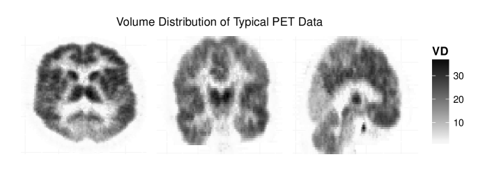
Real neuroscience data sets involve a very large number of time series ($\sim 200,000$ per brain), which are typically somewhat heterogeneous. Figure 2 shows estimates of $V_{D}=\sum_{j=1}^{m}\phi_{j}/\theta_{j}$ from a typical PET scan (generated using SMC2 as will be discussed later). Robustness is therefore especially important. An application-specific MCMC algorithm was developed for this problem in Zhou et al. (2013). A significant amount of tuning of the algorithms was required to obtain good results. The results shown in Figure 2 are very close to those of Zhou et al. (2013) but, as is shown later, they were obtained with almost no manual tuning effort and at similar computational cost.

For SMC and PMCMC algorithms, the requirement of robustness means that the algorithm must be able to calibrate itself automatically to different data (and thus different posterior surfaces). A sequence of distributions which performs well for one time series may not perform even adequately for another series. Specification of proposal scales that produces fast-mixing kernels for one data series may lead to slow mixing for another. In the following experiment, we will use a single simulated time series, and choose schedules that performs both well and poorly for this particular time series. The objective is to see if the algorithm can recover from a relatively poorly specified schedule and obtain reasonably accurate results.

4.2.1 Results

In this example we focus on the comparison between SMC2 and PMCMC. We also consider parallelized implementations of algorithms. In this case, due to its relatively small number of chains, PMCMC can be parallelized completely (and often cannot fully utilize the hardware capability if a naïve approach to parallelization is taken; while we appreciate that more sophisticated parallelization strategies are possible, these depend instrinsicially upon the model under investigation and the hardware employed and given our focus on automatic and general algorithms, we don’t consider such strategies here). The PMCMC algorithm under this setting is implemented such that each chain is updated at each iteration. Further, for the SMC algorithms, we consider two cases. In the first we can parallelize the algorithm completely (in the sense that each core has a single particle associated with it). In this setting we use a relatively small number of particles and a larger number of time steps. In the second, we need a few passes to process a large number of particles at each time step, and accordingly we use fewer time steps to maintain the same total computation time. These two settings allow us to investigate the trade-off between the number of particles and time steps. In both implementations, we consider three schedules, $\alpha(t/T)=t/T$ (linear), $\alpha(t/T)=(t/T)^{5}$ (prior), and $\alpha(t/T)=1-(1-t/T)^{5}$ (posterior). In addition, the adaptive schedule based upon CESS is also implemented for the SMC2 algorithm.

Results from 100 replicate runs of the two algorithms under various regimes can be found in Tables 4 and 5 for the marginal likelihood and Bayes factor estimates, respectively. The SMC algorithms consistently outperforms the PMCMC algorithms in the parallel settings. The Monte Carlo SD of SMC algorithms is typically of the order of one fifth of the corresponding estimates from PMCMC in most scenarios. In some settings with the smaller number of samples, the two algorithms can be comparable. Also at the lowest computational costs, the samplers with more time steps and fewer particles outperform those with the converse configuration by a fairly large margin in terms of estimator variance. It shows that with limited resources, ensuring the similarity of consecutive distributions, and thus good mixing, can be more beneficial than a larger number of particles. However, when the computational budget is increased, the difference becomes negligible. The robustness of SMC to the change of schedules is again apparent.

It can also be seen that increasing the number of distributions not only reduces the bias the path sampling estimator (as seen in the previous example), but also reduces the variances considerably given the same number of particles. On the other hand, increasing the number particles can only reduce the variance of the estimates, in accordance with the central limit theorem; see Del Moral et al. (2006b) for the standard estimator and extensions for the path sampling estimator, Proposition 1 in the supplementary material. (as the bias arises from numerical integration approximation of the path sampling estimator.)

Proposal scales			Manual			Adaptive
Annealing scheme			Prior (5)	Posterior (5)	Adaptive
$T$	$N$	Algorithm	Marginal likelihood estimates ($\log p(\bm{y}|{M_{k}})\pm\text{SD}$)
$500$	$30$	PMCMC	$-39.1\pm 0.56$	$-926.8\pm 376.99$
$500$	$192$	SMC2-DS	$\color[rgb]{0,0,1}\it-39.2\pm 0.25$	$\color[rgb]{0,0,1}\it-39.7\pm 1.06$	$\color[rgb]{0,0,1}\it-39.2\pm 0.18$	$\color[rgb]{1,0,0}\bf-39.1\pm 0.12$
		SMC2-PS	$\color[rgb]{0,0,1}\it-39.2\pm 0.25$	$-91.3\pm 21.69$	$\color[rgb]{0,0,1}\it-39.2\pm 0.18$	$-39.1\pm 0.13$
$100$	$960$	SMC2-DS	$-39.3\pm 0.36$	$-40.6\pm 1.41$	$-39.2\pm 0.31$	$-39.2\pm 0.19$
		SMC2-PS	$-39.3\pm 0.35$	$302.1\pm 46.29$	$-39.3\pm 0.31$	$-39.2\pm 0.18$
$5000$	$30$	PMCMC	$-39.3\pm 0.21$	$-917.6\pm 129.54$
$5000$	$192$	SMC2-DS	$-39.2\pm 0.09$	$\color[rgb]{0,0,1}\it-39.2\pm 0.20$	$-39.2\pm 0.08$	$-39.1\pm 0.04$
		SMC2-PS	$-39.2\pm 0.09$	$-43.8\pm 2.13$	$-39.2\pm 0.08$	$-39.1\pm 0.04$
$1000$	$960$	SMC2-DS	$\color[rgb]{0,0,1}\it-39.2\pm 0.08$	$-39.2\pm 0.31$	$\color[rgb]{0,0,1}\it-39.2\pm 0.07$	$\color[rgb]{1,0,0}\bf-39.2\pm 0.03$
		SMC2-PS	$\color[rgb]{0,0,1}\it-39.2\pm 0.08$	$-65.7\pm 5.54$	$\color[rgb]{0,0,1}\it-39.2\pm 0.07$	$\color[rgb]{1,0,0}\bf-39.2\pm 0.03$

Table 4: Marginal likelihood estimates of two component PET model. $T$: Number of distributions in SMC and number of iterations used for inference in PMCMC. $N$: Number of particles in SMC and number chains in PMCMC. The PMCMC and SMC with $N=192$ are completely $N$-way parallelized. SMC with $N=960$ are $N/5$-way parallelized. Italic: Minimum variance for the same computational cost and the same proposal scales and annealing schemes. Bold: Minimum variance for the same computaitonal cost and all proposal scales and annealing schemes.

Proposal scales			Manual			Adaptive
Annealing scheme			Prior (5)	Posterior (5)	Adaptive
$T$	$N$	Algorithm	Bayes factor estimates ($\log B_{2,1}\pm\text{SD}$)
$500$	$30$	PMCMC	$1.7\pm 0.62$	$-70.9\pm 525.79$
$500$	$192$	SMC2-DS	$\color[rgb]{0,0,1}\it 1.6\pm 0.27$	$\color[rgb]{0,0,1}\it 1.3\pm 1.13$	$\color[rgb]{0,0,1}\it 1.6\pm 0.20$	$\color[rgb]{1,0,0}\bf 1.6\pm 0.15$
		SMC2-PS	$\color[rgb]{0,0,1}\it 1.6\pm 0.27$	$-3.9\pm 30.02$	$\color[rgb]{0,0,1}\it 1.6\pm 0.20$	$\color[rgb]{1,0,0}\bf 1.6\pm 0.15$
$100$	$960$	SMC2-DS	$1.6\pm 0.37$	$0.5\pm 1.55$	$1.6\pm 0.34$	$1.6\pm 0.21$
		SMC2-PS	$1.6\pm 0.37$	$-13.1\pm 66.30$	$1.6\pm 0.33$	$1.6\pm 0.21$
$5000$	$30$	PMCMC	$1.6\pm 0.24$	$-60.3\pm 198.10$
$5000$	$192$	SMC2-DS	$1.6\pm 0.10$	$\color[rgb]{0,0,1}\it 1.6\pm 0.23$	$1.6\pm 0.09$	$1.6\pm 0.05$
		SMC2-PS	$1.6\pm 0.10$	$1.3\pm 2.98$	$1.6\pm 0.09$	$1.6\pm 0.05$
$1000$	$960$	SMC2-DS	$\color[rgb]{0,0,1}\it 1.6\pm 0.09$	$1.6\pm 0.33$	$\color[rgb]{0,0,1}\it 1.6\pm 0.08$	$\color[rgb]{1,0,0}\bf 1.6\pm 0.04$
		SMC2-PS	$\color[rgb]{0,0,1}\it 1.6\pm 0.09$	$-0.2\pm 6.63$	$\color[rgb]{0,0,1}\it 1.6\pm 0.08$	$\color[rgb]{1,0,0}\bf 1.6\pm 0.04$

Table 5: Bayes factor $B_{2,1}$ estimates of two component PET model. $T$: Number of distributions in SMC and number of iterations used for inference in PMCMC. $N$: Number of particles in SMC and number chains in PMCMC. The PMCMC and SMC with $N=192$ are completely $N$-way parallelized. SMC with $N=960$ are $N/5$-way parallelized. Italic: Minimum variance for the same computational cost and the same schedule. Bold: Minimum variance for the same computational cost and all schedules.

Effects of adaptive schedule

A set of samplers with adaptive schedules are also used. Due to the nature of the schedule, it cannot be controlled to have exactly the same number of time steps as non-adaptive procedures. However, the CESS was controlled such that the average number of time steps are comparable with the fixed schedules and in most cases slightly less than the fixed numbers.

It is found that, with little computational overhead, adaptive schedules do provide the best results (or very nearly so) and do so without user intervention. The reduction of Monte Carlo SD varies among different configurations. For moderate or larger number of distributions, a reduction about 50% was observed. In addition, it shall be noted that, in this example, the bias of path sampling estimates are much more sensitive to the schedules than the previous Gaussian mixture model example. A vanilla linear schedule does not provide a low bias estimator at all even when the number of distributions is increased to a considerably larger number. The prior schedule though provides a nearly unbiased estimator, there is no clear theoretical evidence showing that this shall work for other situations. The adaptive schedule, without any manual calibration, can provide a nearly unbiased estimator, even when path-sampling is employed, in addition to potential variance reduction.

Bias reduction for path sampling estimator

As seen in Tables 4 and 5, a bad choice of schedule $\alpha(t/T)$ can results in considerable bias for the basic path sampling estimator, here for SMC2-PS but the problem is independent of the mechanism by which the samples are obtained. Increasing the number of iterations can reduce this bias but at the cost of additional computation time. As outlined in Section 3.3.1, in the case of the SMC algorithms discussed here, it is possible to reduce the bias without increasing computational cost significantly. To demonstrate the bias reduction effect, we constructed SMC sampler for the above PET example with only $1,000$ particles and about $20$ iterations specified using the CESS based adaptive strategy. The path sampling estimator was approximated using Equation (3.13) as well as other higher order numerical integration or by integrating over a grid that contains $\{\alpha_{t}\}$ at which the samples was generated. The results are shown in Table 6

	Number of grid points (compared to sampled iterations)
Integration rule	$\times 1$	$\times 2$	$\times 4$	$\times 8$
Trapezoid	$-52.2\pm 5.01$	$-45.5\pm 1.93$	$-42.1\pm 1.21$	$-40.5\pm 1.06$
Simpson	$-43.2\pm 1.39$	$-41.0\pm 1.10$	$-40.0\pm 1.04$	$-39.4\pm 1.04$
Simpson $3/8$	$-42.1\pm 1.21$	$-40.5\pm 1.06$	$-39.7\pm 1.04$	$-39.3\pm 1.04$
Boole	$-40.9\pm 1.09$	$-39.9\pm 1.04$	$-39.4\pm 1.04$	$-39.2\pm 1.05$

Table 6: Path sampling estimator of marginal likelihood of two component PET model. The estimator was approximated using samples from SMC2 algorithm with $1,000$ particles and $20$ iterations, with different numerical integration strategies. Large sample result (see Table 4) provide an estimate of $-39.2$.

Real data results

Finally, the methodology of SMC2-PS was applied to measured positron emission tomography data using the same compartmental setup as in the simulations. The data shown in Figure 2 comes from a study into opioid receptor density in Epilepsy, with the data being described in detail in Jiang et al. (2009). It is expected that there will be considerable spatial smoothness to the estimates of the volume of distribution, as this is in line with the biology of the system being somewhat regional. Some regions will have much higher receptor density while others will be much lower, yielding higher and lower values of the volume of distribution, respectively. While we did not impose any spatial smoothness but rather estimated the parameters independently for each time series at each spatial location, as can be seen, smooth spatial estimates of the volume of distribution consistent with neurological understanding were found using the approach. This method is computationally feasible for the entire brain on a voxel-by-voxel basis, due to the ease of parallelization of the SMC algorithm. In the analysis performed here, 1000 particles were used, along with an adaptive schedule using a constant $\text{CESS}^{\star}=0.999$, resulting in about 180 to 200 intermediate distributions. The model selection results are very close to those obtained by a previous study of the same data (Zhou et al., 2013), although the present approach requires much less implementation effort and has roughly the same computational cost.

4.3 Summary

These two illustrative applications and the GMM example in the supplementary material have essentially shown three aspects of using SMC as a generic tool for Bayesian model selection. First, as seen in the GMM example, all the different variants of SMC proposed, including both direct and path sampling versions, produce results which are competitive with other model selection methods such as RJMCMC and PMCMC. In addition, in this somewhat simple example, SMC2 performs well, and leads to low variance estimates with no appreciable bias. The effect of adaptation was studied more carefully in the nonlinear ODE example, and it was shown that using both adaptive selection of distributions as well as adaptive proposal variances leads to very competitive algorithms, even against those with significant manual tuning. This suggests that an automatic process of model selection using SMC2 is possible. In the final example, considering the easy parallelization of algorithms such as SMC2 suggests that great gains in variance estimation can be made using settings such as GPU computing for application where computational resources are of particular importance (such as in image analysis as in the PET example). It is also clear that the negligible cost of the bias reduction techniques described means that one should always consider using these to reduce the bias inherent in path sampling estimation. As can also be seen in the supplementary material, there is theoretical justification, in terms of a central limit theorem, available for the path sampling estimator considered in SMC2-PS.

5 Discussion

It has been shown that SMC is an effective Monte Carlo method for Bayesian inference for the purpose of model comparison. Three approaches have been outlined and investigated in several challenging scenarios. The proposed strategy is always competitive and often substantially outperforms the state of the art in this area.

Among the three approaches developed, SMC1 is applicable to very general settings. It can provide a robust alternative to RJMCMC when inference on a countable collection of models is required (and could be readily combined with the approach of Jasra et al. (2008) at the expense of a little additional implementation effort). However, like all Monte Carlo methods involving between model moves, it can be difficult to design efficient algorithms in practice. The SMC3 algorithm is conceptually appealing. However, specifying a suitable sequence of distributions between two posterior distributions is challeging.

The SMC2 algorithm, which only involves within-model simulation, is most straightforward to implement in many interesting problems and has been shown to be exceedingly robust in many settings. As it depends largely upon a collection of within-model MCMC moves, any existing MCMC algorithms can be reused in the SMC2 framework. However, much less tuning is required because the algorithm is fundamentally less sensitive to the mixing of the Markov kernel and it is possible to implement effective adaptive strategies at little computational cost. With adaptive placement of the intermediate distributions and specification of the MCMC kernel proposals, it provides a robust and nearly automatic model comparison method.

Compared to the PMCMC algorithm, SMC2 has greater flexibility in the specification of distributions. Unlike PMCMC, where the number and placement of distributions can affect the mixing speed and hence performance considerably, increasing the number of distributions will always benefit a SMC sampler given the same number of particles. Compared to its no-resampling variant, it has been shown that SMC samplers with resampling can reduce the variance of normalizing constant estimates considerably.

Even after three decades of intensive development, no Monte Carlo method can solve the Bayesian model comparison problem completely automatically without any manual tuning. However, SMC algorithms and the adaptive strategies demonstrated in this paper show that even for realistic, interesting problems, these samplers can provide good results with very minimal tuning and few design difficulties. For many applications, they could already be used as near automatic, robust solutions. For more challenging problems, they can serve as solid foundation for the design of dedicated algorithms.

Supplementary Material

Available from authors.

References

- Andrieu et al. (2010) Andrieu, C., A. Doucet, and R. Holenstein (2010). Particle Markov chain Monte Carlo. Journal of Royal Statistical Society B 72(3), 269–342.
- Atchadé et al. (2010) Atchadé, Y. F., G. O. Roberts, and J. S. Rosenthal (2010). Towards optimal scaling of Metropolis-coupled Markov chain Monte Carlo. Statistics and Computing 21(4), 555–568.
- Bartolucci et al. (2006) Bartolucci, F., L. Scaccia, and A. Mira (2006). Efficient Bayes factor estimation from the reversible jump output. Biometrika 93(1), 41–52.
- Bernardo and Smith (1994) Bernardo, J. M. and A. F. M. Smith (1994). Bayesian Theory. Wiley Series in Probability and Statistics. John Wiley & Sons, Inc.
- Beskos et al. (2013) Beskos, A., A. Jasra, and A. H. Thiéry (2013). On the convergence of adaptive sequential Monte Carlo methods. Mathematics e-print 1306.6462, ArXiv.
- Calderhead and Girolami (2009) Calderhead, B. and M. Girolami (2009). Estimating Bayes factors via thermodynamic integration and population MCMC. Computational Statistics & Data Analysis 53(12), 4028–4045.
- Cappé et al. (2007) Cappé, O., S. J. Godsill, and E. Moulines (2007). An overview of existing methods and recent advances in sequential Monte Carlo. Proceedings of the IEEE 95(5), 899–924.
- Carlin and Chib (1995) Carlin, B. P. and S. Chib (1995). Bayesian model choice via Markov chain Monte Carlo methods. Journal of Royal Statistical Society B 57(3), 473–484.
- Chib (1995) Chib, S. (1995). Marginal likelihood from the Gibbs output. Journal of the American Statistical Association 90(432), 1313–1321.
- Chib and Jeliazkov (2001) Chib, S. and I. Jeliazkov (2001). Marginal likelihood from the Metropolis-Hastings output. Journal of the American Statistical Association 96(453), 270–281.
- Chopin (2002) Chopin, N. (2002). A sequential particle filter method for static models. Biometrika 89(3), 539–552.
- Del Moral (1996) Del Moral, P. (1996). Nonlinear filtering: interacting particle solution. Markov Processes and Related Fields 4(2), 555–580.
- Del Moral (2004) Del Moral, P. (2004). Feynman-Kac Formulae: Genealogical and Interacting Particle Systems with Applications. New York: Springer-Verlag.
- Del Moral et al. (2006a) Del Moral, P., A. Doucet, and A. Jasra (2006a). Sequential Monte Carlo methods for Bayesian computation. In Bayesian Statistics 8. Oxford University Press.
- Del Moral et al. (2006b) Del Moral, P., A. Doucet, and A. Jasra (2006b). Sequential Monte Carlo samplers. Journal of Royal Statistical Society B 68(3), 411–436.
- Del Moral et al. (2012) Del Moral, P., A. Doucet, and A. Jasra (2012). On adaptive resampling strategies for sequential Monte Carlo methods. Bernoulli 18(1), 252–278.
- Doucet and Johansen (2011) Doucet, A. and A. M. Johansen (2011). A tutorial on particle filtering and smoothing: Fifteen years later. In The Oxford Handbook of Non-linear Filtering. Oxford University Press.
- Fan et al. (2008) Fan, Y., D. Leslie, and M. P. Wand (2008). Generalised linear mixed model analysis via sequential Monte Carlo sampling. Electronic Journal of Statistics 2, 916–938.
- Fearnhead and Taylor (2010) Fearnhead, P. and B. Taylor (2010). An adaptive sequential Monte Carlo sampler. Mathematics Preprint 1005.1193v2, ArXiv.
- Friel et al. (2012) Friel, N., M. Hurn, and J. Wyse (2012). Improving power posterior estimation of statistical evidence. ArXiv 1209.3198, 1–24.
- Gelfand and Dey (1994) Gelfand, A. E. and D. K. Dey (1994). Bayesian model choice: Asymptotics and exact calculations. Journal of Royal Statistical Society B 56(3), 501–514.
- Gelman and Meng (1998) Gelman, A. and X.-L. Meng (1998). Simulating normalizing constants: From importance sampling to bridge sampling to path sampling. Statistical Science 13(2), 163–185.
- Geyer (1991) Geyer, C. (1991). Monte Carlo maximum likelihood. In Keramigas (Ed.), Proceedings of Computing Science and Statistics: The 23rd Symposium on the Interface, Fairfax, pp. 156–161. Interface Foundation.
- Godsill (2001) Godsill, S. J. (2001). On the relationship between Markov chain Monte Carlo for model uncerntainty. Journal of Computational and Graphical Statistics 10(2), 230–248.
- Green (1995) Green, P. J. (1995). Reversible jump Markov chain Monte Carlo computation and Bayesian model determination. Biometrika 82(4), 711–732.
- Gunn et al. (2002) Gunn, R. N., S. R. Gunn, F. E. Turkheimer, J. A. D. Aston, and V. J. Cunningham (2002). Positron emission tomography compartmental models: A basis pursuit strategy for kinetic modeling. Journal of Cerebral Blood Flow & Metabolism 22(12), 1425–1439.
- Jasra et al. (2008) Jasra, A., A. Doucet, D. A. Stephens, and C. C. Holmes (2008). Interacting sequential Monte Carlo samplers for trans-dimensional simulation. Computational Statistics & Data Analysis 52(4), 1765–1791.
- Jasra et al. (2010) Jasra, A., D. A. Stephens, A. Doucet, and T. Tsagaris (2010, December). Inference for Lévy-Driven Stochastic Volatility Models via Adaptive Sequential Monte Carlo. Scandinavian Journal of Statistics 38(1), 1–22.
- Jasra et al. (2007a) Jasra, A., D. A. Stephens, and C. C. Holmes (2007a). On population-based simulation for static inference. Statistics and Computing 17(3), 263–279.
- Jasra et al. (2007b) Jasra, A., D. A. Stephens, and C. C. Holmes (2007b). Population-based reversible jump Markov chain Monte Carlo. Biometrika 94(4), 787–807.
- Jiang et al. (2009) Jiang, C.-R., J. A. D. Aston, and J.-L. Wang (2009). Smoothing dynamic positron emission tomography time courses using functional principal components. NeuroImage 47(1), 184–193.
- Johansen et al. (2006) Johansen, A. M., P. Del Moral, and A. Doucet (2006). Sequential Monte Carlo samplers for rare events. In Proceedings of the 6th International Workshop on Rare Event Simulation, pp. 256–267.
- Johansen et al. (2008) Johansen, A. M., A. Doucet, and M. Davy (2008). Particle methods for maximum likelihood estimation in latent variable models. Statistics and Computing 18(1), 47–57.
- Karagiannis and Andrieu (2013) Karagiannis, G. and C. Andrieu (2013). Annealed importance sampling reversible jump MCMC algorithms. Journal of Computational and Graphical Statistics 22(3), 623–648.
- Kong et al. (1994) Kong, A., J. S. Liu, and W. H. Wong (1994). Sequential imputations and Bayesian missing data problems. Journal of the American Statistical Association 89(425), 278–288.
- Lee et al. (2010) Lee, A., C. Yau, M. B. Giles, A. Doucet, and C. C. Holmes (2010). On the utility of graphics cards to perform massively parallel simulation of advanced Monte Carlo methods. Journal of Computational and Graphical Statistics 19(4), 769–789.
- Liang and Wong (2001) Liang, F. and W. H. Wong (2001, June). Real-parameter evolutionary Monte Carlo with applications to Bayesian mixture models. Journal of the American Statistical Association 96(454), 653–666.
- Marinari and Parisi (1992) Marinari, E. and G. Parisi (1992). Simulated tempering: a new Monte Carlo scheme. Europhysics Letters 19(6), 451–458.
- Neal (1994) Neal, R. M. (1994). Discussion of “Approximate Bayesian inference with the weighted likelihood bootstrap” by Newton and Raftery. Journal of the Royal Statistical Society, Series B 56(1), 41–42.
- Neal (2001) Neal, R. M. (2001). Annealed importance sampling. Statistics and Computing 11(2), 125–139.
- Newton and Raftery (1994) Newton, M. A. and A. E. Raftery (1994). Approximate Bayesian inference with the weighted likelihood bootstrap. Journal of Royal Statistical Society B 56(1), 3–48.
- Peters et al. (2010) Peters, G., K. Hayes, and G. Hossack (2010). Ecological non-linear state space model selection via adaptive particle Markov chain Monte Carlo (AdPMCMC). Mathematics Preprint 1005.2238, ArXiv.
- Peters (2005) Peters, G. W. (2005). Topics in sequential Monte Carlo samplers. Master’s thesis, University of Cambridge, Department of Engineering.
- Raftery et al. (2006) Raftery, A. E., M. A. Newton, J. M. Satagopan, and P. N. Krivitsky (2006, November). Estimating the Integrated Likelihood via Posterior Simulation Using the Harmonic Mean Identity. In Bayesian Statistics 8, pp. 1–45. Oxford University Press.
- Robert (2007) Robert, C. P. (2007). The Bayesian Choice: From Decision-theoretic Foundations to Computational Implementation (2nd ed.). New York: Springer.
- Roberts and Tweedie (1996) Roberts, G. O. and R. L. Tweedie (1996). Exponential convergence of Langevin distributions and their discrete approximations. Bernoulli 2(4), 341–363.
- Rousset and Stoltz (2006) Rousset, M. and G. Stoltz (2006). Equilibrium sampling from nonequilibrium dynamics. Journal of Statistical Physics 123(6), 1251–1272.
- Schäfer and Chopin (2013) Schäfer, C. and N. Chopin (2013). Sequential Monte Carlo on large binary sampling spaces. Statistics and Computing 23(2), 163–184.
- Schwarz (1978) Schwarz, G. (1978). Estimating the dimension of a model. The Annals of Statistics 6(2), 461–464.
- Schweizer (2012) Schweizer, N. (2012, April). Non-asymptotic error bounds for sequential mcmc and stability of feynman-kac propagators. Mathematics Preprint 1204.2382, ArXiv, New York.
- Vyshemirsky and Girolami (2008) Vyshemirsky, V. and M. A. Girolami (2008). Bayesian ranking of biochemical system models. Bioinformatics 24(6), 833–839.
- Zhou (2013) Zhou, Y. (2013). vSMC: Parallel sequential Monte Carlo in C++. Mathematics e-print 1306.5583, ArXiv.
- Zhou et al. (2013) Zhou, Y., J. A. D. Aston, and A. M. Johansen (2013, May). Bayesian model comparison for compartmental models with applications in positron emission tomography. Journal of Applied Statistics 40(5), 993–1016.
- Zhou et al. (2012) Zhou, Y., A. M. Johansen, and J. A. D. Aston (2012). Bayesian model selection via path-sampling sequential Monte Carlo. In Proceedings of IEEE Statistical Signal Procesing Workshop, Ann Arbor, Michigan, USA, pp. 245–248.