Cosmic variance and the measurement of the local Hubble parameter

Abstract

There is an approximately 9% discrepancy, corresponding to 2.4$\sigma$, between two independent constraints on the expansion rate of the universe: one indirectly arising from the cosmic microwave background and baryon acoustic oscillations, and one more directly obtained from local measurements of the relation between redshifts and distances to sources. We argue that by taking into account the local gravitational potential at the position of the observer this tension – strengthened by the recent Planck results – is partially relieved and the concordance of the standard model of cosmology increased. We estimate that measurements of the local Hubble constant are subject to a cosmic variance of about 2.4% (limiting the local sample to redshifts $z>0.010$) or 1.3% (limiting it to $z>0.023$), a more significant correction than that taken into account already. Nonetheless, we show that one would need a very rare fluctuation to fully explain the offset in the Hubble rates. If this tension is further strengthened, a cosmology beyond the standard model may prove necessary.

Introduction

We can only observe the universe from our own position, which is – in terms of cosmological scales – fixed and lying in a gravitational potential the value of which possibly cannot be probed Valkenburg et al. (2012). If the observer could move around in the universe, they would measure the variation of local parameters, a variation caused by observing from locations with different values of the gravitational potential. However, as we cannot measure this unavoidable variation, there is a cosmic variance on physical parameters that are potentially sensitive to the local spacetime around the observer. One such parameter is the local expansion rate.

In this Letter we discuss how the locally measured expansion rate is offset from the global average expansion rate of the universe by the value of the gravitational potential at the observer. By considering the statistics of the distribution of matter in the universe, we derive the distribution of the gravitational potential at the observer, and, consequently, the expected distribution of the offset of the local expansion rate with respect to the global expansion rate. On one hand this analysis (partially) relieves the tension between existing local and global measurements of the expansion rate. On the other hand, our results suggest that local measurements of the Hubble parameter are limited to a minimum systematic error of a few percent, which should be included in the error budget of such measurements.

Constraints on the Hubble constant

The most recent measurement of the local Hubble parameter performed by considering recession velocities of objects around us reports a value of $H_{0}^{\text{local}}=73.8\pm 2.4$ km s^-1 Mpc^-1 Riess et al. (2011), while the Planck 2013 analysis gives $H_{0}^{\text{\tiny CMB}}=67.80\pm 0.77$ km s^-1 Mpc^-1 (Ade et al., 2013, Table 5), assuming a spatially flat $\Lambda$CDM model (a homogeneous universe with a cosmological constant $\Lambda$ and cold dark matter) and fitting to observations of the cosmic microwave background (CMB) and baryon acoustic oscillations (BAO) only. These two independent measurements give a discrepancy of approximately 9%, corresponding to 2.4$\sigma$. It is worth stressing that the recent Planck results strengthened this tension, which is only marginal, at 2.0$\sigma$, when the 9-year WMAP data is used Hinshaw et al. (2012). The 9% disagreement between the expansion rates could be a statistical fluke or instead a hint for a neglected systematic error. Here we take the second point of view. Local fluctuations of the Hubble parameter are indeed to be expected as a consequence of the density perturbations abundant in the late non-linear universe. In particular, a higher $H_{0}^{\text{local}}$ will be observed if we happen to live inside an underdensity (see e.g. Bonvin et al. (2006); Hui and Greene (2006); Cooray and Caldwell (2006); Neill et al. (2007); Li and Schwarz (2008); Hunt and Sarkar (2010); Sinclair et al. (2010); Umeh et al. (2011); Amendola et al. (2010); Valkenburg (2012a); Wiegand and Schwarz (2012); Romano and Chen (2011); Valkenburg and Bjaelde (2012); Marra et al. (2013); Ben-Dayan et al. (2013a); Kalus et al. (2012); Ben-Dayan et al. (2013b); Valkenburg et al. (2013) for studies of the effect of a neglected inhomogeneity on cosmological parameters). It is therefore natural to ask if the tension between $H_{0}^{\text{local}}$ and $H_{0}^{\text{\tiny CMB}}$ can be relieved if a local underdensity consistent with large-scale structure is taken into account in the analysis.

It is interesting to note that the possibility of living in a local underdense “Hubble bubble” has been considered before. Ref. Jha et al. (2007) found indeed that the Hubble parameter estimated from supernovae Ia (SNe) within 74$h^{-1}$Mpc is $6.5\%\pm 1.8\%$ higher than the Hubble parameter measured from SNe outside this region (see also Haugboelle et al. (2007); Conley et al. (2007)). The analysis of Riess et al. (2011) considers this issue and tries to correct for it; we will discuss this later. The topic of a local Hubble bubble dates back to the 90’s, see e.g. Turner et al. (1992); Suto et al. (1995); Shi et al. (1996); Shi and Turner (1998); Wang et al. (1998); Zehavi et al. (1998); Giovanelli et al. (1999) for previous work on the cosmic variance of the local Hubble parameter.

The Hubble bubble model

To tackle this problem we take the simplest approach, that is, we model the inhomogeneity by means of the Hubble bubble model, which is the basis of the so-called spherical “top-hat” collapse Kolb and Turner (1990). The idea is to carve out of the FLRW background a sphere of matter which is then compressed or diluted so as to obtain a toy model of the inhomogeneity with a slightly different FLRW solution. At the junction of the two metrics, the density is discontinuous and the description could be improved by means of the spherically symmetric Lemaître-Tolman-Bondi (LTB) solution of Einstein’s equation Lemaître (1933); Tolman (1934); Bondi (1947). For our purposes, however, the Hubble bubble model suffices, as we are not interested in the junction between inhomogeneity and background.

A straightforward prediction of the Hubble bubble model is that an adiabatic perturbation in density causes a perturbation in the expansion rate given by:

$$\frac{\delta H}{H}=-\frac{1}{3}\;\frac{\delta\rho}{\rho}\;f(\Omega_{m})\;\Theta\!\left(\frac{\delta\rho}{\rho},\Omega_{m}\right)\,,$$ (1)

where all quantities are evaluated at the present time. The function $f(\Omega_{m})$ is the growth rate and embodies the effect of a non-negligible cosmological constant. During matter domination one has $f=1$, and the standard relation is recovered. In Fig. 1 we show the function $\Theta\left(\tfrac{\delta\rho}{\rho},\Omega_{m}\right)$, which parametrizes the effect of values of $\delta\rho/\rho$ approaching the non-linear regime, computed by means of the $\Lambda$LTB model Marra and Paakkonen (2010); Valkenburg (2012b). For linear contrasts, $|\delta\rho/\rho|\ll 1$, we have $\Theta\simeq 1$ and Eq. (1) becomes a linear relation between perturbations in the density and perturbations in the expansion rate.

Figure 1: Function $\Theta$ which corrects the relation of Eq. (1) when the density contrast is not linear. The plot assumes the Planck+BAO best-fit value of $\Omega_{m}=0.3086$, but the dependence of $\Theta$ on cosmological parameters is very weak.

The local measurements of the Hubble constant from Ref. Riess et al. (2011) use standard candles within the redshift range bounded by $z_{\rm min}=0.010$ (or 0.023) and $z_{\rm max}=0.1$. Therefore, we need to know the typical contrast of a perturbation that extends over a redshift in this range. We take a conservative approach and consider density perturbations stemming from a standard matter power spectrum $P(k)$ with Planck+BAO best-fit parameters. Consequently, we know that the mean square of the density perturbation in a sphere of radius $R$ around any point today – and so also around us – is

$$\sigma_{R}^{2}\equiv\left(\frac{\delta M}{M}\right)^{2}=\int_{0}^{\infty}\frac{k^{2}\mathrm{d}k}{2\pi^{2}}\,P(k)\left[\frac{3j_{1}(R\,k)}{R\,k}\right]^{2}\,,$$ (2)

where $M$ is the mass enclosed by a sphere of radius $R$ and $j_{1}$ is the spherical Bessel function of the first kind.

Next we assume that perturbations in the density field follow a gaussian distribution $p_{\rm gau}$ with the variance given by $\sigma_{R}^{2}$ of Eq. (2):

$$p_{\rm gau}(x)=\frac{1}{\sigma_{R}\sqrt{2\pi}}\;e^{-\tfrac{x^{2}}{2\,\sigma_{R}^{2}}}\,,$$ (3)

with $x\equiv\delta\rho/\rho$. In Fig. 2 we plot the 68%, 95% and 99.7% confidence-level fluctuations on the local Hubble parameter, as well as the 1-$\sigma$ band relative to the value $H_{0}^{\text{local}}/H_{0}^{\text{\tiny CMB}}-1$, which shows the 2.4-$\sigma$ tension discussed above.

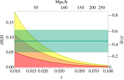
Figure 2: The 68%, 95% and 99.7% confidence-level probabilities of gaussian matter fluctuations (right vertical axis) and consequently of the local Hubble parameter (left vertical axis), as a function of co-moving size of the matter fluctuation (top ticks) or, equivalently, redshift (bottom ticks). The relation between $\delta H/H$ and $\delta\rho/\rho$ is given by Eq. (1). The range $z_{\rm min}\leq z\leq z_{\rm max}$ corresponds to the range of observation of Riess et al. (2011). Also shown is the 1-$\sigma$ emerald band relative to the value $H_{0}^{\text{local}}/H_{0}^{\text{\tiny CMB}}-1$, which shows the 2.4$\sigma$ tension between CMB and local measurements of the Hubble constant.

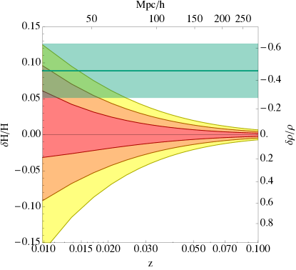
Figure 3: The 68%, 95% and 99.7% confidence-level probabilities of log-normally distributed matter fluctuations (right vertical axis) and consequently of the local Hubble parameter (left vertical axis), as a function of co-moving size of the matter fluctuation (top ticks) or, equivalently, redshift (bottom ticks). As in Fig. 2 we show the 1-$\sigma$ band relative to the value $H_{0}^{\text{local}}/H_{0}^{\text{\tiny CMB}}-1$.

In reality, nonlinear matter fluctuations are better described by a lognormal distribution Coles and Jones (1991):

$$p_{\rm logn}(x)=\frac{\exp\left[-\frac{\left(\log\left(\sigma^{2}_{R}+1\right)+2\log(x+1)\right)^{2}}{8\log\left(\sigma^{2}_{R}+1\right)}\right]}{\sqrt{2\pi}(x+1)\sqrt{\log\left(\sigma^{2}_{R}+1\right)}}\,,$$ (4)

which has zero mean, variance $\sigma^{2}_{R}$ and support $(-1,\infty]$ – in agreement with the fact that $\delta\rho/\rho>-1$. Moreover, for $\sigma_{R}\rightarrow 0$ it approaches the gaussian distribution of Eq. (3). In Fig. 3 we show the 68%, 95% and 99.7% confidence level fluctuations of the local Hubble parameter induced by log-normally distributed matter perturbations. We show separately the case for both over- and under-densities as they are no longer symmetric when using a skewed distribution such as Eq. (4). Using the log-normal distribution, we see that local voids at a low redshift are actually more likely than they would appear from a gaussian distribution. From here on, we will use the superscripts $+,-$ to refer to the distinct distributions of positive and negative perturbations and their properties, in particular the mean systematic error $\sigma^{\pm}_{H_{0}}$. For the symmetric gaussian distribution we of course have $\sigma_{H_{0}}^{+}=\sigma_{H_{0}}^{-}$.

Discussion

In order to estimate the mean systematic error on local determinations of the Hubble constant we average the 68% confidence level on $\delta H/H$ over the survey range:

$$\sigma_{H_{0}}^{\pm}=\left[\int_{z_{\rm min}}^{z_{\rm max}}\mathrm{d}z\,W_{\rm SN}(z)\,\left(\frac{\delta H^{\pm}}{H^{\phantom{\pm}}}\right)^{2}\right]^{1\over 2}\,.$$ (5)

In the equation above, the quantity $W_{\rm SN}(z)$ represents the redshift distribution of the SNe used in Riess et al. (2011), which is peaked at the lower redshifts. It is important to stress at this point that we are assuming that the SNe are isotropically distributed over the sky. This implies that we are neglecting the effect of the anisotropic distribution of the sources, which could increase sizably the magnitude of the cosmic variance. We list in Table 1 the numerical values of Eq. (5) for combinations of cases where either the gaussian distribution of Eq. (3) or the skewed log-normal distribution of Eq. (4) is used.

As $\delta H/H$ is naturally larger at lower redshift, the value of $\sigma_{H_{0}}$ depends strongly on $W_{\rm SN}(z)$ and, in particular, on $z_{\rm min}$ and $z_{\rm max}$. If one were to extend the upper range $z_{\rm max}$ then the cosmic variance $\sigma_{H_{0}}$ could be reduced at the cost that the uncertainty in the values of the cosmological parameters $\Omega_{\text{m}},\Omega_{\Lambda}$, negligible in the current analysis, would begin to play a role. Alternatively, one could reduce the effect of the cosmic variance by increasing the lower cutoff $z_{\rm min}$. As discussed earlier, Ref. Jha et al. (2007) claims that the expansion rate estimated from SNe within 74$h^{-1}$Mpc (corresponding approximately to $z=0.023$) is $6.5\%\pm 1.8\%$ larger than the one measured from SNe outside this region. Consequently, one can alleviate the Hubble bubble effect by adopting $z_{\rm min}=0.023$ Riess et al. (2011). In Table 1, we also show the values of $\sigma_{H_{0}}$ corresponding to this choice. The median redshift of the SN redshift distribution is $z_{\rm median}\simeq 0.025$ if $z_{\rm min}=0.010$ is used, and $z_{\rm median}\simeq 0.033$ if $z_{\rm min}=0.023$ is adopted instead. Also, from Figures 2 and 3 one can see that this mismatch of 6.5% can be explained by a local inhomogeneity in agreement with the standard model at about $2\sigma_{R}$.

Case		Density Contrast Distribution	$z_{\text{min}}$		$\sigma_{H_{0}}^{+}$	$\sigma_{H_{0}}^{-}$	$\delta H_{0}^{+}\left(\frac{\rm km/s}{\rm Mpc}\right)$		Adding errors linearly	Adding errors in quadrature
I		$p_{\rm gau\phantom{\tiny c\!}}$ of Eq. (3)	$0.010$		2.1%	2.1%	1.58		$\Delta H=1.6\sigma$	$\Delta H=2.1\sigma$
II		$p_{\rm logn}$ of Eq. (4)	$0.010$		2.4%	1.7%	1.79		$\Delta H=1.5\sigma$	$\Delta H=2.1\sigma$
III		$p_{\rm gau\phantom{\tiny c\!}}$ of Eq. (3)	$0.023$		1.2%	1.2%	0.90		$\Delta H=1.9\sigma$	$\Delta H=2.4\sigma$
IV		$p_{\rm logn}$ of Eq. (4)	$0.023$		1.3%	1.1%	0.97		$\Delta H=1.8\sigma$	$\Delta H=2.4\sigma$

Table 1: Cosmic variance $\sigma_{H_{0}}^{\pm}$ of the local Hubble parameter calculated using Eq. (5). $p_{\text{gau}}$ and $p_{\text{logn}}$ denote the statistical distribution used to describe the density contrast, $\delta\rho/\rho$, gaussian (3) or lognormal (4). $z_{\text{min}}$ denotes the minimum redshift of the SNe included in the sample. The gaussian distribution has symmetric errors, $\sigma_{H_{0}}^{+}=\sigma_{H_{0}}^{-}$. The quantity $\delta H_{0}^{+}$ gives the absolute error relative to $\sigma_{H_{0}}^{+}$ for $H_{0}^{\text{local}}$. Finally, $\Delta H\equiv\left|H_{0,\text{unc}}^{\text{local}}-H_{0}^{\text{\tiny CMB}}\right|=2.5\sigma$ describes how much the tension between the CMB and local measurement of $H_{0}$ is reduced when $\sigma_{H_{0}}^{+}$ is included as a systematic error. The quantity $H_{0,\text{unc}}^{\text{local}}$ is the 0.5%-larger uncorrected value of the local Hubble constant, see the main text for more details.

It is now natural to ask how much this additional error from the cosmic variance of our local gravitational potential can relieve the tension of 9% between the central values of the two observations discussed at the beginning. Before proceeding, however, we should point out that Ref. Riess et al. (2011) besides limiting in most of the analysis the sample to $z_{\rm min}=0.023$, also tries to address the cosmic variance uncertainty by correcting each SN Ia on the Hubble diagram for the expected perturbation of its redshift as determined from the IRAS PSCz density field Branchini et al. (1999), in particular by adopting the model B05 of Ref. Neill et al. (2007). The result of this velocity correction causes the final value of $H_{0}$ to decrease by $0.5\%\pm 0.1\%$. While this approach is in our opinion the right way to proceed so as to deal with the cosmic variance, in light of the tension between $H_{0}^{\text{\tiny CMB}}$ and $H_{0}^{\text{local}}$ and the uncertainties in the model of Ref. Neill et al. (2007), we think it is worth considering the case in which one does not use the results of Neill et al. (2007) and more conservatively estimates the variance stemming from standard inhomogeneities. We therefore compare the global $H_{0}^{\text{\tiny CMB}}$ to the 0.5%-larger uncorrected value of $H_{0,\text{unc}}^{\text{local}}=74.2\pm 2.4$ km s^-1 Mpc^-1. This slightly increases the tension which is now $\Delta H\equiv\left|H_{0,\text{unc}}^{\text{local}}-H_{0}^{\text{\tiny CMB}}\right|=2.5\sigma$. As the error from cosmic variance is systematic in nature it should be kept separate from the statistical one. Just to give a rough estimate, we list in Table 1 how much the tension is reduced by adding the errors linearly or in quadrature. When using the log-normal distribution we employ the value $\sigma_{H_{0}}^{+}$ as $H_{0}^{\text{local}}>H_{0}^{\text{\tiny CMB}}$.

Conclusions

The simple analysis of this Letter carries two messages. The first is that local measurements of the Hubble parameter are limited to the minimum systematic error $\delta H_{0}^{+}$ listed in Table 1. These results qualitatively agree with previous estimations of the cosmic variance of the local expansion rate (see e.g. Shi and Turner (1998); Wang et al. (1998); Kalus et al. (2012)).

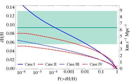
Figure 4: Probability of having an inhomogeneity that induces a $\delta H/H$ (left vertical axis) or $\delta H$ (right vertical axis) larger than a given value for the cases listed in the legend and in Table 1. Also shown is the 1-$\sigma$ band relative to the value $H_{0,\text{unc}}^{\text{local}}/H_{0}^{\text{\tiny CMB}}-1$.

The second point is that by including the effect of a local inhomogeneity – in particular a local underdensity – the tension between CMB and local measurements of the Hubble constant is alleviated, even though only partially. One can quantify the remaining tension by estimating the probability that inhomogeneities stemming from a standard matter power spectrum can explain the 9% discrepancy. We show in Fig. 4 the result for the four cases discussed in Table 1: it is evident that one needs a very rare large-scale structure to explain away the offset in the Hubble rates. If this tension is further increased, a cosmology beyond the standard model may prove necessary.

Of course, a more thorough analysis is needed in order to precisely quantify the effect of the local inhomogeneity on measurements of the expansion rate, possibly by introducing the effect of perturbations of the local gravitational potential directly in the first steps of the data analysis, as in Riess et al. (2011). Nonetheless, the results of this Letter provide a quick and easy way – equations (1) to (5) – to estimate the systematic error $\sigma_{H_{0}}$, which can be specialized to a given survey by using the corresponding distribution of standard candles $W_{\rm SN}(z)$.

Finally, in the present era of “precision” cosmology it is of crucial importance to fully understand the source of this offset in the Hubble rates, if it is a mere systematic error or new physics. If one neglects this issue, a fit of a cosmological experiment at large scale combined with local measurements of the Hubble constant biases the extracted cosmological parameters e.g. the equation of state of dark energy and the effective number of relativistic degrees of freedom. On the other hand, disregarding local measurements on the basis of this disagreement might potentially obscure a hint of cosmology beyond the standard model. This is clearly shown by the analysis of the Planck collaboration, see e.g. Eqs (91-93) in Ade et al. (2013).

References

- Valkenburg et al. (2012) W. Valkenburg, V. Marra, and C. Clarkson, (2012), arXiv:1209.4078 [astro-ph.CO] .
- Riess et al. (2011) A. G. Riess, L. Macri, S. Casertano, H. Lampeitl, H. C. Ferguson, et al., Astrophys.J. 730, 119 (2011), arXiv:1103.2976 [astro-ph.CO] .
- Ade et al. (2013) P. Ade et al. (Planck Collaboration), (2013), arXiv:1303.5076 [astro-ph.CO] .
- Hinshaw et al. (2012) G. Hinshaw, D. Larson, E. Komatsu, D. Spergel, C. Bennett, et al., (2012), arXiv:1212.5226 [astro-ph.CO] .
- Bonvin et al. (2006) C. Bonvin, R. Durrer, and M. A. Gasparini, Phys.Rev. D73, 023523 (2006), arXiv:astro-ph/0511183 [astro-ph] .
- Hui and Greene (2006) L. Hui and P. B. Greene, Phys.Rev. D73, 123526 (2006), arXiv:astro-ph/0512159 [astro-ph] .
- Cooray and Caldwell (2006) A. Cooray and R. R. Caldwell, Phys.Rev. D73, 103002 (2006), arXiv:astro-ph/0601377 [astro-ph] .
- Neill et al. (2007) J. D. Neill, M. J. Hudson, and A. J. Conley, Astrophys.J. 661, L123 (2007), arXiv:0704.1654 [astro-ph] .
- Li and Schwarz (2008) N. Li and D. J. Schwarz, Phys.Rev. D78, 083531 (2008), arXiv:0710.5073 [astro-ph] .
- Hunt and Sarkar (2010) P. Hunt and S. Sarkar, Mon.Not.Roy.Astron.Soc. 401, 547 (2010), arXiv:0807.4508 [astro-ph] .
- Sinclair et al. (2010) B. Sinclair, T. M. Davis, and T. Haugbolle, Astrophys.J. 718, 1445 (2010), arXiv:1006.0911 [astro-ph.CO] .
- Umeh et al. (2011) O. Umeh, J. Larena, and C. Clarkson, JCAP 1103, 029 (2011), arXiv:1011.3959 [astro-ph.CO] .
- Amendola et al. (2010) L. Amendola, K. Kainulainen, V. Marra, and M. Quartin, Phys.Rev.Lett. 105, 121302 (2010), arXiv:1002.1232 [astro-ph.CO] .
- Valkenburg (2012a) W. Valkenburg, JCAP 1201, 047 (2012a), arXiv:1106.6042 [astro-ph.CO] .
- Wiegand and Schwarz (2012) A. Wiegand and D. J. Schwarz, Astron.Astrophys. 538, A147 (2012), arXiv:1109.4142 [astro-ph.CO] .
- Romano and Chen (2011) A. E. Romano and P. Chen, JCAP 1110, 016 (2011), arXiv:1104.0730 [astro-ph.CO] .
- Valkenburg and Bjaelde (2012) W. Valkenburg and O. E. Bjaelde, Mon.Not.Roy.Astron.Soc. 424, 495 (2012), arXiv:1203.4567 [astro-ph.CO] .
- Marra et al. (2013) V. Marra, M. Paakkonen, and W. Valkenburg, Mon.Not.Roy.Astron.Soc. , (2013), arXiv:1203.2180 [astro-ph.CO] .
- Ben-Dayan et al. (2013a) I. Ben-Dayan, M. Gasperini, G. Marozzi, F. Nugier, and G. Veneziano, Phys.Rev.Lett. 110, 021301 (2013a), arXiv:1207.1286 [astro-ph.CO] .
- Kalus et al. (2012) B. Kalus, D. J. Schwarz, M. Seikel, and A. Wiegand, (2012), arXiv:1212.3691 [astro-ph.CO] .
- Ben-Dayan et al. (2013b) I. Ben-Dayan, M. Gasperini, G. Marozzi, F. Nugier, and G. Veneziano, (2013b), arXiv:1302.0740 [astro-ph.CO] .
- Valkenburg et al. (2013) W. Valkenburg, M. Kunz, and V. Marra, (2013), arXiv:1302.6588 [astro-ph.CO] .
- Jha et al. (2007) S. Jha, A. G. Riess, and R. P. Kirshner, Astrophys.J. 659, 122 (2007), arXiv:astro-ph/0612666 [astro-ph] .
- Haugboelle et al. (2007) T. Haugboelle, S. Hannestad, B. Thomsen, J. Fynbo, J. Sollerman, et al., Astrophys.J. 661, 650 (2007), arXiv:astro-ph/0612137 [astro-ph] .
- Conley et al. (2007) A. J. Conley, R. Carlberg, J. Guy, D. Howell, S. Jha, et al., Astrophys.J. 664, L13 (2007), arXiv:0705.0367 [astro-ph] .
- Turner et al. (1992) E. L. Turner, R. Cen, and J. P. Ostriker, Astron.J. 103, 1427 (1992).
- Suto et al. (1995) Y. Suto, T. Suginohara, and Y. Inagaki, Prog.Theor.Phys. 93, 839 (1995), arXiv:astro-ph/9412090 [astro-ph] .
- Shi et al. (1996) X. Shi, L. M. Widrow, and L. J. Dursi, Mon.Not.Roy.Astron.Soc. 281, 565 (1996), arXiv:astro-ph/9506120 [astro-ph] .
- Shi and Turner (1998) X.-D. Shi and M. S. Turner, Astrophys.J. 493, 519 (1998), arXiv:astro-ph/9707101 [astro-ph] .
- Wang et al. (1998) Y. Wang, D. N. Spergel, and E. L. Turner, Astrophys.J. 498, 1 (1998), arXiv:astro-ph/9708014 [astro-ph] .
- Zehavi et al. (1998) I. Zehavi, A. G. Riess, R. P. Kirshner, and A. Dekel, Astrophys.J. 503, 483 (1998), arXiv:astro-ph/9802252 [astro-ph] .
- Giovanelli et al. (1999) R. Giovanelli, D. Dale, M. Haynes, E. Hardy, and L. Campusano, Astrophys.J. 525, 25 (1999), arXiv:astro-ph/9906362 [astro-ph] .
- Kolb and Turner (1990) E. W. Kolb and M. S. Turner, Front.Phys. 69, 1 (1990).
- Lemaître (1933) G. Lemaître, Ann.Soc.Sci.Bruxelles 53, 51 (1933).
- Tolman (1934) R. C. Tolman, Proc.Nat.Acad.Sci. 20, 169 (1934).
- Bondi (1947) H. Bondi, Mon.Not.Roy.Astron.Soc. 107, 410 (1947).
- Linder (2005) E. V. Linder, Phys.Rev. D72, 043529 (2005), arXiv:astro-ph/0507263 [astro-ph] .
- Valkenburg (2012b) W. Valkenburg, Gen.Rel.Grav. 44, 2449 (2012b), arXiv:1104.1082 [gr-qc] .
- Marra and Paakkonen (2010) V. Marra and M. Paakkonen, JCAP 1012, 021 (2010), arXiv:1009.4193 [astro-ph.CO] .
- Coles and Jones (1991) P. Coles and B. Jones, Mon.Not.Roy.Astron.Soc. 248, 1 (1991).
- Branchini et al. (1999) E. Branchini, L. Teodoro, C. Frenk, I. Schmoldt, G. Efstathiou, et al., Mon.Not.Roy.Astron.Soc. 308, 1 (1999), arXiv:astro-ph/9901366 [astro-ph] .
- Riess et al. (2012) A. G. Riess, J. Fliri, and D. Valls-Gabaud, Astrophys.J. 745, 156 (2012), arXiv:1110.3769 [astro-ph.CO] .