Hydrodynamic instability in warped astrophysical discs

Abstract

Warped astrophysical discs are usually treated as laminar viscous flows, which have anomalous properties when the disc is nearly Keplerian and the viscosity is small: fast horizontal shearing motions and large torques are generated, which cause the warp to evolve rapidly, in some cases at a rate that is inversely proportional to the viscosity. However, these flows are often subject to a linear hydrodynamic instability, which may produce small-scale turbulence and modify the large-scale dynamics of the disc. We use a warped shearing sheet to compute the oscillatory laminar flows in a warped disc and to analyse their linear stability by the Floquet method. We find widespread hydrodynamic instability deriving from the parametric resonance of inertial waves. Even very small, unobservable warps in nearly Keplerian discs of low viscosity can be expected to generate hydrodynamic turbulence, or at least wave activity, by this mechanism.

1 Introduction

In the companion paper (Ogilvie & Latter, 2013, hereafter Paper I), we have revisited the basic theory of warped astrophysical discs, in which the orbital plane varies with radius. We have introduced a local model, a warped shearing sheet, that is suitable for detailed analytical and numerical studies of warped discs. As well as rederiving the nonlinear theory of laminar viscous discs (Ogilvie, 1999) by a simpler route, we have shown how the local model can be used more generally to compute the internal torque that drives the large-scale evolution of the shape and mass distribution of the disc, thereby connecting the local and global dynamics.

An important feature of a warped disc is that the orbiting fluid experiences a horizontal pressure gradient, antisymmetric about the midplane, that oscillates at the orbital frequency (or nearly so, if the shape of the disc is slowly varying in a non-rotating frame of reference). This force generates horizontal shearing motions, which are resonantly amplified if the disc is Keplerian (or nearly so), owing to the coincidence of the orbital and epicyclic frequencies. By transporting angular momentum in the radial direction, these motions provide an internal torque that causes an anomalously rapid evolution of the disc.

Existing treatments of warped discs represent these internal motions, if at all, as laminar flows. In Papaloizou & Pringle (1983) their amplitude is limited only by viscous damping, with the result that the internal torque, and the rate of evolution of the warp, are inversely proportional to the viscosity. (In this context, viscosity is usually taken to represent the effects of unresolved physical processes such as small-scale turbulence.) In a propagating bending wave (Papaloizou & Lin, 1995) the time-dependence ensures that the internal motions have a finite amplitude, even in the absence of viscosity, but the linear theory often predicts hypersonic flows above and below the midplane. The same is true in the nonlinear theory of Ogilvie (1999), which we have revisited in Paper I.

It has previously been noted that these oscillatory shear flows are likely to be linearly unstable (Papaloizou & Terquem, 1995; Gammie, Goodman & Ogilvie, 2000). To the best of our knowledge, instability has not been detected in any of the global numerical simulations of warped discs (many of which are cited in Paper I), probably because they have insufficient spatial resolution or too much viscosity, either explicit or numerical, to allow the unstable modes to develop. Therefore these simulations also represent warped discs as laminar flows and may be missing an important physical process.

Hydrodynamic instability is likely to lead to turbulence, or at least significant wave activity, and to alter the internal flows in a warped disc. We expect an important modification of the large-scale dynamics of warped discs, and this is one reason why we are motivated to make a detailed study of the instability. Another reason is that it will provide a source of hydrodynamic activity in Keplerian discs, especially in poorly ionized regions where the magnetorotational instability (MRI) is inoperative. These secondary motions could be important in determining many of the physical properties of these regions, for example by stirring up the dead zones of protoplanetary discs. Note that only a very small warp may be required to excite these motions, owing to the resonant amplification of the internal flows in a Keplerian disc. Such small but dynamically significant warps may not be directly observable even with high-resolution imaging. More generally, we are interested in the interplay between hydrodynamic instability resulting from a warp and other sources of turbulence and transport in astrophysical discs, including the MRI.

The likelihood of a local linear hydrodynamic instability in warped discs was noted by Papaloizou & Terquem (1995), and the first explicit calculations were made by Gammie, Goodman & Ogilvie (2000). Gammie, Goodman & Ogilvie (2000) did not represent the warp itself, but considered the horizontal shearing motions, oscillating at the local orbital frequency, that are driven by the warp. These motions are linearly unstable when the associated shear rate is sufficiently large compared to the viscosity of the fluid, the instability taking the form of a parametric resonance of inertial waves. In nonlinear local simulations, the shearing motions decay as they lose energy to inertial waves. Torkelsson et al. (2000) studied the decay of similar flows in the presence of magnetohydrodynamic (MHD) turbulence driven by the MRI.

An effect related to the parametric instability of warped discs is the mode-coupling process investigated by Kato (2004) and Ferreira & Ogilvie (2008). This allows a warp in the inner part of a disc around a black hole to excite inertial waves that are trapped near the radius at which the epicyclic frequency is maximal, and which may be related to observed high-frequency quasi-periodic oscillations from accreting black holes.

In the local hydrodynamic and MHD simulations of Gammie, Goodman & Ogilvie (2000) and Torkelsson et al. (2000), the horizontal shearing motions were imposed as initial conditions and were allowed to decay through instability or interaction with turbulence. However, in order to reach a better understanding of the role of instabilities or turbulence in the dynamics of warped discs, a model is required in which the effect of the warp can be maintained and the dynamics can reach a quasi-steady state. Such a model is provided by the warped shearing sheet defined in Paper I.

To prepare the way for future nonlinear simulations in the warped shearing sheet, we tackle the linear problem in this paper, analysing the hydrodynamic stability of the laminar flows computed in Paper I. Our analysis is closely related to that of Gammie, Goodman & Ogilvie (2000), but is more detailed and is based on the nonlinear laminar flow solutions computed in a warped shearing sheet. We compute the growth rates of the unstable modes and their variation with several parameters. In certain regimes the instability can be clearly identified as a parametric resonance of inertial waves, in agreement with previous work. We also speculate on the nonlinear outcome and its consequences for warped discs, as well as making suggestions for further investigation.

2 Local model and laminar flows

In this section we summarize the equations of Paper I on which our analysis is based. The local model of a warped disc introduced in that paper is based on a circular reference orbit of radius $r_{0}$ and angular velocity $\Omega_{0}$, where the dimensionless rate of orbital shear is $q=-\mathrm{d}\ln\Omega/\mathrm{d}\ln r$, equal to ${\textstyle\frac{3}{2}}$ for Keplerian orbits. The initial construction is identical to the standard shearing sheet or box and leads to the hydrodynamic equations

$$\mathrm{D}u_{x}-2\Omega_{0}u_{y}=2q\Omega_{0}^{2}x-\partial_{x}h,$$ (1)

$$\mathrm{D}u_{y}+2\Omega_{0}u_{x}=-\partial_{y}h,$$ (2)

$$\mathrm{D}u_{z}=-\Omega_{0}^{2}z-\partial_{z}h,$$ (3)

$$\mathrm{D}h=-c_{\mathrm{s}}^{2}(\partial_{x}u_{x}+\partial_{y}u_{y}+\partial_{z}u_{z}),$$ (4)

where

$$\mathrm{D}=\partial_{t}+u_{x}\partial_{x}+u_{y}\partial_{y}+u_{z}\partial_{z}$$ (5)

is the Lagrangian derivative and ${\mn@boldsymbol{u}}$ is the velocity. For simplicity, we consider an isothermal gas for which

$$p=c_{\mathrm{s}}^{2}\rho,$$ (6)

where $c_{\mathrm{s}}=\mathrm{constant}$ is the isothermal sound speed, and we make use of the pseudo-enthalpy

$$h=c_{\mathrm{s}}^{2}\ln\rho+\mathrm{constant}.$$ (7)

To represent a warped disc we introduce the warped shearing coordinates

$$t^{\prime}=t,$$ (8)

$$x^{\prime}=x,$$ (9)

$$y^{\prime}=y+q\tau x,$$ (10)

$$z^{\prime}=z+|\psi|\cos\tau\,x,$$ (11)

where

$$\tau=\Omega_{0}t^{\prime}=\Omega_{0}t$$ (12)

is the orbital phase and $|\psi|$ is the dimensionless warp amplitude. These coordinates follow the warped orbital motion. Partial derivatives transform according to

$$\partial_{t}=\partial_{t}^{\prime}+q\Omega_{0}x\partial_{y}^{\prime}-|\psi|\Omega_{0}\sin\tau\,x\partial_{z}^{\prime},$$ (13)

$$\partial_{x}=\partial_{x}^{\prime}+q\tau\,\partial_{y}^{\prime}+|\psi|\cos\tau\,\partial_{z}^{\prime},$$ (14)

$$\partial_{y}=\partial_{y}^{\prime},$$ (15)

$$\partial_{z}=\partial_{z}^{\prime},$$ (16)

so that

$$\mathrm{D}=\partial_{t}^{\prime}+v_{x}\partial_{x}^{\prime}+(v_{y}+q\tau v_{x})\partial_{y}^{\prime}+(v_{z}+|\psi|\cos\tau\,v_{x})\partial_{z}^{\prime},$$ (17)

where

$$v_{x}=u_{x},$$ (18)

$$v_{y}=u_{y}+q\Omega_{0}x,$$ (19)

$$v_{z}=u_{z}-|\psi|\Omega_{0}\sin\tau\,x$$ (20)

are the relative velocity components.

The hydrodynamic equations are therefore transformed into

$$\mathrm{D}v_{x}-2\Omega_{0}v_{y}=-(\partial_{x}^{\prime}+q\tau\,\partial_{y}^{\prime}+|\psi|\cos\tau\,\partial_{z}^{\prime})h,$$ (21)

$$\mathrm{D}v_{y}+(2-q)\Omega_{0}v_{x}=-\partial_{y}^{\prime}h,$$ (22)

$$\mathrm{D}v_{z}+|\psi|\Omega_{0}\sin\tau\,v_{x}=-\Omega_{0}^{2}z^{\prime}-\partial_{z}^{\prime}h,$$ (23)

$$\mathrm{D}h=-c_{\mathrm{s}}^{2}[(\partial_{x}^{\prime}+q\tau\,\partial_{y}^{\prime}+|\psi|\cos\tau\,\partial_{z}^{\prime})v_{x}+\partial_{y}^{\prime}v_{y}+\partial_{z}^{\prime}v_{z}].$$ (24)

These equations are easily extended to include a dynamic shear viscosity $\mu=\alpha p/\Omega_{0}$ and a dynamic bulk viscosity $\mu_{\mathrm{b}}=\alpha_{\mathrm{b}}p/\Omega_{0}$, where $\alpha$ and $\alpha_{\mathrm{b}}$ are constant dimensionless coefficients. We do not write out the viscous terms explicitly, however.

The simplest solutions of equations (21)–(24), extended to include viscosity, are laminar flows of the form

$$v_{x}(z^{\prime},t^{\prime})=u(\tau)\Omega_{0}z^{\prime},$$ (25)

$$v_{y}(z^{\prime},t^{\prime})=v(\tau)\Omega_{0}z^{\prime},$$ (26)

$$v_{z}(z^{\prime},t^{\prime})=w(\tau)\Omega_{0}z^{\prime},$$ (27)

$$h(z^{\prime},t^{\prime})=c_{\mathrm{s}}^{2}f(\tau)-{\textstyle\frac{1}{2}}\Omega_{0}^{2}z^{\prime 2}g(\tau),$$ (28)

where $u$, $v$, $w$, $f$ and $g$ are dimensionless $2\pi$-periodic functions that satisfy the equations

$$\mathrm{d}_{\tau}u+(w+|\psi|\cos\tau\,u)u-2v=|\psi|\cos\tau\,g$$ (29)

$$-(\alpha_{\mathrm{b}}+{\textstyle\frac{1}{3}}\alpha)|\psi|\cos\tau\,g(w+|\psi|\cos\tau\,u)$$

$$-\alpha g[|\psi|\sin\tau+(1+|\psi|^{2}\cos^{2}\tau)u],$$

$$\mathrm{d}_{\tau}v+(w+|\psi|\cos\tau\,u)v+(2-q)u$$ (30)

$$=-\alpha g[-q|\psi|\cos\tau+(1+|\psi|^{2}\cos^{2}\tau)v],$$

$$\mathrm{d}_{\tau}w+(w+|\psi|\cos\tau\,u)w+|\psi|\sin\tau\,u=g-1$$ (31)

$$-(\alpha_{\mathrm{b}}+{\textstyle\frac{1}{3}}\alpha)g(w+|\psi|\cos\tau\,u)$$

$$-\alpha g[|\psi|^{2}\sin\tau\cos\tau+(1+|\psi|^{2}\cos^{2}\tau)w],$$

$$\mathrm{d}_{\tau}f=-(w+|\psi|\cos\tau\,u),$$ (32)

$$\mathrm{d}_{\tau}g=-2(w+|\psi|\cos\tau\,u)g,$$ (33)

where $\mathrm{d}_{\tau}$ denotes the ordinary derivative $\mathrm{d}/\mathrm{d}\tau$. Numerical solutions of these equations are presented in Paper I.

3 Stability of laminar flows

3.1 Simple expectations

Before embarking on a detailed analysis of the stability of the laminar flows, we make some very simple estimates, omitting factors of order unity.

We are usually interested in discs that are nearly Keplerian ($|q-{\textstyle\frac{3}{2}}|\ll 1$) and of low viscosity ($\alpha\ll 1$). In such discs the horizontal laminar flows are resonant and can reach large amplitudes, even if the warp amplitude $|\psi|$ is small.

The magnitude of $u$ (or $v$, which is similar) can be simply estimated as follows. The horizontal motion is a linear oscillator, whose natural frequency is the epicyclic frequency. It is forced at the orbital frequency by the horizontal pressure gradients associated with the warp, and is damped by viscosity. The problem is similar to a damped harmonic oscillator forced at, or close to, its natural frequency; the response of the oscillator is limited either by detuning or damping, whichever is larger. When detuning of the resonance due to non-Keplerian rotation is the limiting factor, $u$ scales as $|\psi|/|q-{\textstyle\frac{3}{2}}|$ (valid when this quantity is $\la 1$). When viscous damping of the horizontal flows is the limiting factor, $u$ scales as $|\psi|/\alpha$ (valid when this quantity is $\la 1$). Examples of these scalings can be seen in figs 6 and 7 of Paper I.

These oscillatory shear flows are unstable in the absence of viscosity, and the inviscid growth rate of the instability scales with the shear rate $u\Omega$ (Gammie, Goodman & Ogilvie, 2000). Since the unstable modes have a non-trivial vertical structure and a horizontal wavelength related to the scale-height of the disc, $H$, viscous damping quenches the instability if $\nu/H^{2}\ga u\Omega$, i.e. if $\alpha\ga u$. Therefore (omitting factors of order unity) instability is expected when $|\psi|\ga|q-{\textstyle\frac{3}{2}}|\alpha$ or $\alpha^{2}$, whichever is larger. These are only very rough estimates or scaling relations; detailed results are obtained in Section 3.6 below.

3.2 Linearized equations

To examine the stability of the laminar flows we linearize the basic equations (21)–(24) about the solution (25)–(28), introducing infinitesimal perturbations of the form

$$\mathrm{Re}[\delta{\mn@boldsymbol{v}}(z^{\prime},\tau)\exp(\mathrm{i}k_{x}^{\prime}x^{\prime}+\mathrm{i}k_{y}^{\prime}y^{\prime})],$$ (34)

etc., where $(k_{x}^{\prime},k_{y}^{\prime})$ is a real horizontal wavevector. The linearized equations admit solutions of this plane-wave form because the basic equations (21)–(24) from which they are derived do not contain $x^{\prime}$ or $y^{\prime}$ explicitly, and the basic state about which we are linearizing is also independent of $x^{\prime}$ and $y^{\prime}$. Using the relations (9) and (10) between the primed and unprimed horizontal coordinates, we find

$$\exp(\mathrm{i}k_{x}^{\prime}x^{\prime}+\mathrm{i}k_{y}^{\prime}y^{\prime})=\exp(\mathrm{i}k_{x}x+\mathrm{i}k_{y}y),$$ (35)

where

$$(k_{x},k_{y})=(k_{x}^{\prime}+qk_{y}^{\prime}\tau,k_{y}^{\prime})$$ (36)

is a wavevector that may depend on time. If $k_{y}\neq 0$ then $k_{x}$ depends linearly on $\tau$ and we have a shearing wave, which corresponds to a non-axisymmetric spiral disturbance in the global geometry. If $k_{y}=0$ then $k_{x}=k_{x}^{\prime}$ is a constant: the wave is axisymmetric and does not shear.

We also adopt units in which $\Omega_{0}=1$ and $c_{\mathrm{s}}=1$, meaning that the unit of length is the scale-height $c_{\mathrm{s}}/\Omega_{0}$ of an unwarped disc and the unit of time is $\Omega_{0}^{-1}$. The linearized equations in the absence of viscosity then take the form

$$\mathcal{D}\delta v_{x}+(\delta v_{z}+|\psi|\cos\tau\,\delta v_{x})u-2\,\delta v_{y}$$ (37)

$$=-(\mathrm{i}k_{x}+|\psi|\cos\tau\,\partial_{z}^{\prime})\delta h,$$

$$\mathcal{D}\delta v_{y}+(\delta v_{z}+|\psi|\cos\tau\,\delta v_{x})v+(2-q)\delta v_{x}=-\mathrm{i}k_{y}\delta h,$$ (38)

$$\mathcal{D}\delta v_{z}+(\delta v_{z}+|\psi|\cos\tau\,\delta v_{x})w+|\psi|\sin\tau\,\delta v_{x}=-\partial_{z}^{\prime}\delta h,$$ (39)

$$\mathcal{D}\delta h-(\delta v_{z}+|\psi|\cos\tau\,\delta v_{x})gz^{\prime}=-\mathrm{i}k_{x}\delta v_{x}$$ (40)

$$-|\psi|\cos\tau\,\partial_{z}^{\prime}\delta v_{x}-\mathrm{i}k_{y}\delta v_{y}-\partial_{z}^{\prime}\delta v_{z},$$

where

$$\mathcal{D}=\partial_{\tau}+\mathrm{i}(k_{x}u+k_{y}v)z^{\prime}+(w+|\psi|\cos\tau\,u)z^{\prime}\partial_{z}^{\prime}.$$ (41)

For an axisymmetric wave ($k_{y}=0$), $k_{x}$ is constant and the coefficients of the linearized equations have a periodic dependence on $\tau$, with period $2\pi$. For a shearing wave ($k_{y}\neq 0$), the coefficients are non-periodic because $k_{x}$ depends linearly on $\tau$.

The associated equation for the energy of the perturbation is (assuming suitable boundary conditions in $z$)

$$\mathrm{d}_{\tau}\int\rho\left({\textstyle\frac{1}{2}}|\delta{\mn@boldsymbol{v}}|^{2}+{\textstyle\frac{1}{2}}|\delta h|^{2}\right)\mathrm{d}z^{\prime}$$ (42)

$$=-\mathrm{Re}\int\rho\bigg{[}|\delta v_{x}|^{2}|\psi|\cos\tau\,u+\delta v_{x}^{*}\delta v_{y}(-q+|\psi|\cos\tau\,v)$$

$$\qquad\qquad\qquad+\delta v_{x}^{*}\delta v_{z}(|\psi|\sin\tau+|\psi|\cos\tau\,w+u)$$

$$\qquad\qquad\qquad+\delta v_{y}^{*}\delta v_{z}v+|\delta v_{z}|^{2}w\bigg{]}\mathrm{d}z^{\prime}.$$

The right-hand side represents the exchange of energy with the laminar flow and the orbital shear through Reynolds stresses. This equation can be used to bound the growth rate of the perturbation, as discussed in Appendix A.

3.3 Projection on to orthogonal polynomials

To solve equations (37)–(41) we use a Galerkin spectral method, projecting the equations on to a basis of Hermite polynomials

$$\mathrm{He}_{n}(x)=\mathrm{e}^{x^{2}/2}\left(-\frac{\mathrm{d}}{\mathrm{d}x}\right)^{n}\mathrm{e}^{-x^{2}/2},\qquad n=0,1,2,\dots$$ (43)

as used by Okazaki, Kato & Fukue (1987) and many other authors:

$$\delta v_{x}(z^{\prime},\tau)=\sum_{n=0}^{\infty}u_{n}(\tau)\,\mathrm{He}_{n}(z^{\prime}),$$ (44)

$$\delta v_{y}(z^{\prime},\tau)=\sum_{n=0}^{\infty}v_{n}(\tau)\,\mathrm{He}_{n}(z^{\prime}),$$ (45)

$$\delta v_{z}(z^{\prime},\tau)=\sum_{n=1}^{\infty}w_{n}(\tau)\,\mathrm{He}_{n-1}(z^{\prime}),$$ (46)

$$\delta h(z^{\prime},\tau)=\sum_{n=0}^{\infty}h_{n}(\tau)\,\mathrm{He}_{n}(z^{\prime}).$$ (47)

We further define $u_{n}=v_{n}=h_{n}=0$ for $n<0$ and $w_{n}=0$ for $n<1$. The Hermite polynomials, familiar from the quantum harmonic oscillator, are particularly well suited to linear waves in isothermal discs, having a Gaussian weight function that is proportional to the density of an unwarped isothermal disc. Using the relations

$$\mathrm{He}_{n}^{\prime}(x)=n\,\mathrm{He}_{n-1}(x),$$ (48)

$$x\,\mathrm{He}_{n}(x)=\mathrm{He}_{n+1}(x)+n\,\mathrm{He}_{n-1}(x),$$ (49)

we find

$$\mathrm{d}_{\tau}u_{n}+\mathrm{i}(k_{x}u+k_{y}v)[u_{n-1}+(n+1)u_{n+1}]$$ (50)

$$+(w+|\psi|\cos\tau\,u)[nu_{n}+(n+1)(n+2)u_{n+2}]$$

$$+u(w_{n+1}+|\psi|\cos\tau\,u_{n})-2v_{n}=-\mathrm{i}k_{x}h_{n}$$

$$-|\psi|\cos\tau\,(n+1)h_{n+1},$$

$$\mathrm{d}_{\tau}v_{n}+\mathrm{i}(k_{x}u+k_{y}v)[v_{n-1}+(n+1)v_{n+1}]$$ (51)

$$+(w+|\psi|\cos\tau\,u)[nv_{n}+(n+1)(n+2)v_{n+2}]$$

$$+v(w_{n+1}+|\psi|\cos\tau\,u_{n})+(2-q)u_{n}=-\mathrm{i}k_{y}h_{n},$$

$$\mathrm{d}_{\tau}w_{n}+\mathrm{i}(k_{x}u+k_{y}v)(w_{n-1}+nw_{n+1})$$ (52)

$$+(w+|\psi|\cos\tau\,u)[(n-1)w_{n}+n(n+1)w_{n+2}]$$

$$+w(w_{n}+|\psi|\cos\tau\,u_{n-1})+|\psi|\sin\tau\,u_{n-1}=-nh_{n},$$

$$\mathrm{d}_{\tau}h_{n}+\mathrm{i}(k_{x}u+k_{y}v)[h_{n-1}+(n+1)h_{n+1}]$$ (53)

$$+(w+|\psi|\cos\tau\,u)[nh_{n}+(n+1)(n+2)h_{n+2}]$$

$$-(g-1)\{w_{n}+(n+1)w_{n+2}$$

$$\qquad+|\psi|\cos\tau[u_{n-1}+(n+1)u_{n+1}]\}$$

$$=-\mathrm{i}k_{x}u_{n}+|\psi|\cos\tau\,u_{n-1}-\mathrm{i}k_{y}v_{n}+w_{n}.$$

Equations (50), (51) and (53) are to be solved for $n\geq 0$, and equation (52) for $n\geq 1$. The equivalent equations including viscosity are given in Appendix B.

3.4 Solutions in the absence of a warp

In the absence of a warp, $|\psi|=u=v=w=g-1=0$ and the inviscid equations reduce to

$$\mathrm{d}_{\tau}u_{n}-2v_{n}=-\mathrm{i}k_{x}h_{n},$$ (54)

$$\mathrm{d}_{\tau}v_{n}+(2-q)u_{n}=-\mathrm{i}k_{y}h_{n},$$ (55)

$$\mathrm{d}_{\tau}w_{n}=-nh_{n},$$ (56)

$$\mathrm{d}_{\tau}h_{n}=-\mathrm{i}k_{x}u_{n}-\mathrm{i}k_{y}v_{n}+w_{n},$$ (57)

with no coupling between different values of $n$. The same property holds when viscosity is included, but only if $\alpha_{\mathrm{b}}={\textstyle\frac{2}{3}}\alpha$. For axisymmetric waves ($k_{y}=0$), solutions $\propto\mathrm{e}^{-\mathrm{i}\omega\tau}$ exist, with angular frequency $\omega$ given by, in the inviscid case,

$$(-\omega^{2}+n)[-\omega^{2}+2(2-q)]-k_{x}^{2}\omega^{2}=0,$$ (58)

(cf. Okazaki, Kato & Fukue, 1987) and, in the viscous case, a more complicated quartic equation. For $n\geq 1$, the high-frequency solutions of equation (58) have an acoustic character, while the low-frequency solutions have an inertial character. In the case $n=0$, however, the high-frequency solution is the well known two-dimensional (acoustic–inertial) wave, while the low-frequency solution is a zero-frequency vortical mode. The dispersion relation is illustrated in Fig. 1.

 

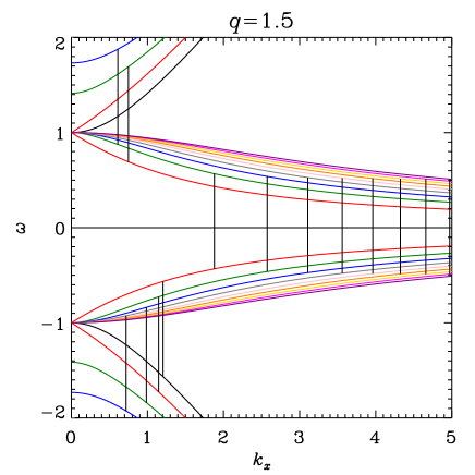
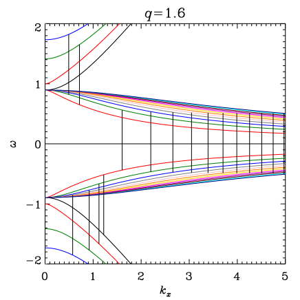
Figure 1: Dispersion relation for axisymmetric waves ($k_{y}=0$) in an unwarped disc in the absence of viscosity, for $q=1.5$ (left) and $q=1.6$ (right). The angular frequency $\omega$ of the waves is in units of $\Omega_{0}$, and the radial wavenumber $k_{x}$ is in units of $\Omega_{0}/c_{\mathrm{s}}$. Different colours indicate different values of the vertical mode number $n$ (0: black, 1: red, 2: green, 3: blue, 4: grey, 5: pink, 6: orange, 7: gold, 8: magenta, 9: purple, 10: maroon, 11: cyan, 12: navy); only modes with $n\leq 9$ are shown for $q=1.5$. Vertical bars of length $1$ show the possible resonant couplings between neighbouring modes. These occur at wavenumbers for which two waves exist with vertical mode numbers $n$ and $n+1$ and with angular frequencies $\omega$ and $\omega+1$.

3.5 Solutions in the presence of a warp

In the presence of a warp, the different Hermite modes are coupled by numerous terms in equations (50)–(53). For example, the terms proportional to $\mathrm{i}(k_{x}u+k_{y}v)$, which derive from the shearing of the waves by the laminar flow, couple neighbouring modes in such a way that an infinite ladder is produced. Indeed, the linearized equations (37)–(40) have no solutions that are strictly polynomial in $z^{\prime}$ in the presence of a warp, because the $\mathrm{i}(k_{x}u+k_{y}v)z^{\prime}$ term in $\mathcal{D}$ generates an infinite power series in $z^{\prime}$. Another type of coupling is provided by the terms proportional to $(g-1)$ in equation (53). These terms arise because the scale-height of the warped disc is time-dependent and different from that of the unwarped disc on which the Hermite polynomials are based. For computational purposes, we truncate the system at some order $N$ by setting $u_{n}$, $v_{n}$, $w_{n}$ and $h_{n}$ to zero for $n\geq N$.

The parametric instability, at least in its simplest form, involves a three-wave coupling between the warp (together with the associated laminar flow) and two inertial waves (Gammie, Goodman & Ogilvie, 2000). The theory is worked out in detail in Appendix C, which is based on an expansion of the equations for small $|\psi|$. In the local model, the warp and its associated laminar flow have radial wavenumber $0$, vertical mode number $1$ and frequency $1$. In order to couple to the warp, the inertial waves should therefore have the same radial wavenumber as each other, while their vertical mode numbers should differ by $1$ (owing to equation 49) and their frequencies should add up to (or differ by) $1$. The density of the spectrum of inertial waves means that there are infinitely many wavenumbers at which this coupling is possible; several of these are illustrated in Fig. 1. (Couplings of acoustic and inertial waves are found not to lead to instability.)

We investigate only axisymmetric waves ($k_{y}=0$) in this paper, looking for instabilities of the laminar flows. As noted above, in this case the linearized equations have coefficients that are $2\pi$-periodic in $\tau$. Our truncated system is a set of $4N-1$ ordinary differential equations (ODEs) and we analyse their solutions using Floquet theory. The characteristic solutions (eigenmodes) of the system of ODEs are $2\pi$-periodic functions of $\tau$ multiplied by $\mathrm{e}^{s\tau}$, where $s$ is a complex growth rate. Choosing a set of $4N-1$ linearly independent initial conditions (by setting all variables except one to zero at $\tau=0$) and integrating the ODEs from $\tau=0$ to $\tau=2\pi$ using a Runge–Kutta method with adaptive stepsize, we evaluate the monodromy matrix that determines the evolution of an arbitrary initial condition over one period. We calculate the eigenvalues of the monodromy matrix, which are the characteristic multipliers $\mathrm{e}^{2\pi s}$, and deduce the complex growth rates. Growing solutions are found when $\mathrm{Re}(s)>0$, and indicate linear instability of the laminar flow. (The imaginary part of $s$ gives the angular frequency of the eigenmode, but this is only defined modulo $1$.)

This numerical method has been verified by reproducing the solutions of the algebraic dispersion relation (58) and its viscous equivalent in the absence of a warp. In the presence of a warp, as described below, it produces results that agree with the analytical calculations of parametric instability in Appendix C. Equations (50)–(53) were also solved with a pseudospectral method, which provides a separate numerical check on the results. As noted above, the characteristic solutions are $2\pi$-periodic functions of $\tau$ multiplied by $\mathrm{e}^{s\tau}$, and if this common factor is extracted from the solutions, a term involving the complex growth rate $s$ appears in each equation. After truncating the number of Hermite modes to $N$, the $\tau$ domain is partitioned into $M$ segments and the $\tau$ derivatives approximated using Fourier collocation. This yields a square matrix of size $4MN$, the eigenvalues of which are the complex growth rates $s$. Good agreement was achieved with the monodromy approach described in the previous paragraph.

3.6 Numerical results

We begin a discussion of the numerical results by considering the relatively simple case of an inviscid non-Keplerian disc with $q=1.6$ and a small warp of amplitude $|\psi|\ll 1$. We compute the growth rate of the fastest growing mode for a range of radial wavenumbers and plot the results in Fig. 2. Instability occurs in bands of $k_{x}$ centred on the wavenumbers predicted by the analysis of three-wave coupling; the red points in the figure show the growth rate at the centre of each band (up to $k_{x}=5$) calculated in Appendix C.1. These growth rates are proportional to $|\psi|$ and tend to a limit as $k_{x}\to\infty$. The bands of instability have a non-zero width, also proportional to $|\psi|$, because the parametric instability permits some detuning. The first few bands are well separated, but eventually they overlap and merge, producing a continuous curve. The limiting growth rate in the continuous regime is twice the limiting value predicted by a single three-wave coupling, because each mode ($n$) can engage simultaneously in three-wave couplings with its two neighbours ($n\pm 1$) (Gammie, Goodman & Ogilvie, 2000). For larger values of $|\psi|$ the theory developed in Appendix C.1 becomes inaccurate.

  

  

  

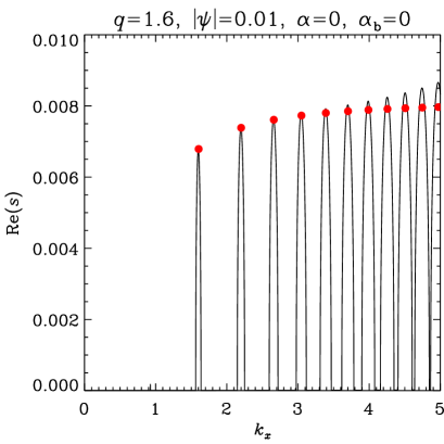
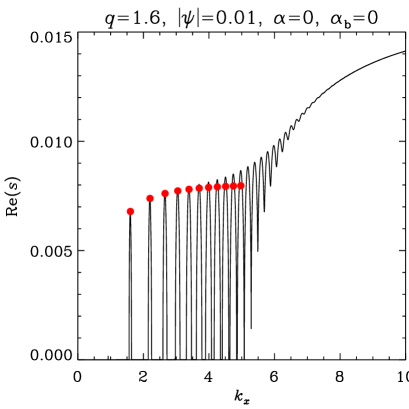
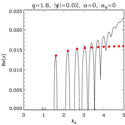
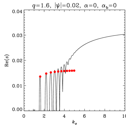
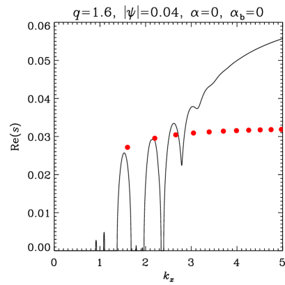
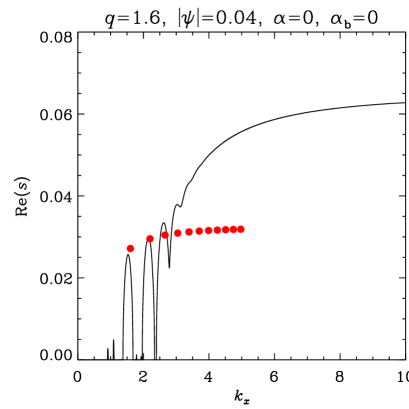
Figure 2: Linear stability of laminar flows for $q=1.6$. The growth rate of the fastest growing mode (in units of $\Omega_{0}$) is plotted versus the radial wavenumber (in units of $\Omega_{0}/c_{\mathrm{s}}$). The red points show the growth rate at the centre of each band of parametric instability (up to $k_{x}=5$), based on the analysis in Appendix C.1. Larger growth rates are obtained where the resonance bands overlap. The left panels require resolutions of up to $N=30$ for convergence. The right panels, which illustrate the behaviour for larger wavenumbers, require up to $N=90$.

In Fig. 3 we show an example of a growing eigenmode, within the first band of parametric instability in the top row of Fig. 2. This mode consists mainly of a superposition of the $n=1$ and $n=2$ inertial waves, coupled resonantly by the warp so as to cause exponential growth. The resulting motion is neither symmetric nor antisymmetric about the midplane, but involves the oblique motions typical of inertial waves below the epicyclic frequency (also seen in fig. 1 of Gammie, Goodman & Ogilvie 2000). The variation of the velocity field with orbital phase is due to the interference of the two inertial waves with different phase speeds $\omega/k_{x}$; the pattern is not significantly distorted by shear, because both the warp amplitude and that of the laminar flow are quite small. By referring to equation (42) and to the first panel of fig. 6 of Paper I (which shows that $u$ is approximately proportional to $\sin\tau$) we can understand how the mode grows: $\delta v_{x}$ and $\delta v_{z}$ are negatively correlated at phase $\tau=\pi/2$ (panel 2) where the shear rate $|\psi|\sin\tau+u$ reaches its positive maximum, and are positively correlated at phase $\tau=3\pi/2$ (panel 4) where the shear rate reaches its negative minimum. The Reynolds stresses associated with this mode are therefore able to release energy from both the warped orbital motion and the laminar flow.

Figure 3: Example of an inviscid growing eigenmode, within the first band of parametric instability in the top row of Fig. 2. Velocity vectors $\delta{\mn@boldsymbol{v}}$, multiplied by $\rho^{1/2}$ to show the distribution of wave energy, are shown in the $x^{\prime}z^{\prime}$ plane at over two radial wavelengths, at orbital phases $\tau=0$, $\pi/2$, $\pi$ and $3\pi/2$.

The situation for a Keplerian disc is more complicated. Viscosity must be included in order to obtain laminar flow solutions, and the analysis of parametric instability is modified, mainly because of the different phase relationships in the laminar flows. Fig. 4 shows some results for very small warps and Fig. 5 for larger, but still probably unobservable, warps. The viscosity parameter $\alpha$ is chosen in each case to be sufficiently large that the laminar flow has a modest amplitude $(|u|<1)$. Distinct bands of parametric instability are clearly visible only for very small $|\psi|$ and $\alpha$, as in the left panel of Fig. 4, where good agreement is found with the analytical calculation in Appendix C.2. Note that viscous damping reduces the growth rate at larger values of $k_{x}$. For larger warp amplitudes, the analytical theory becomes inaccurate and instability occurs in broader ranges of $k_{x}$.

  

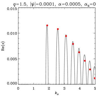
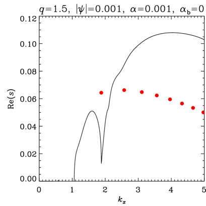
Figure 4: Linear stability of laminar flows for $q=1.5$, including viscosity. The left panel is computed with $N=20$ and the right panel with $N=40$, which are sufficient to provide converged results for this range of $k_{x}$. The red points show the growth rate at the centre of each band of parametric instability, based on the analysis in Appendix C.2, and taking into account viscous damping; this analysis is inaccurate for the right panel. Larger growth rates are obtained where the resonance bands overlap.

  

Figure 5: Continuation of Fig. 5 to larger warp amplitudes. $N=30$ is sufficient for the left panel and $N=80$ for the right panel.

In situations where the laminar flows have large amplitude ($|u|\ga 1$) and the viscosity is small ($\alpha\ll 1$), large growth rates ($\mathrm{Re}(s)\ga 1$) may be expected. However, in this regime the eigenvalues returned by our numerical method do not converge as the truncation order $N$ is increased, and therefore we do not present any such results in this paper. Initially the difficulty takes the form of spurious modes, presumably arising from the truncation of the Hermite basis, with non-convergent growth rates that can exceed those of the genuine modes. Such unwanted solutions can be excluded by comparing the eigenvalues calculated with different truncation orders. Later, however, the entire spectrum fails to converge. The reason for this behaviour is probably that the coupling terms proportional to $\mathrm{i}k_{x}u$ in equations (50)–(53) are strong, and indeed the problem is worse for larger values of $k_{x}$. It may be simply that the Hermite basis, which is designed for wave modes in an unwarped disc, is incapable of handling the modes of a warped disc with strong laminar flows.

It is also possible, however, that modal solutions cease to exist when the laminar flows are too strong, or when the radial wavenumber is too large. After all, it is not obvious why an unwarped isothermal disc supports acoustic and inertial waves whose energy is confined near the midplane. If the vertical gravitational acceleration were constant, instead of being proportional to $z$, there would be a continuous spectrum instead of confined modes. Similarly, in a stably stratified vertical isothermal disc with adiabatic exponent $\gamma>1$, the internal gravity waves are not confined but form a continuous spectrum. In a shearing sheet without radial structure or boundaries, non-axisymmetric eigenmodes do not exist because of the inexorable shear, and are replaced by non-modal solutions. It is possible that the oscillatory shear of a strong laminar flow in a warped disc may prevent the formation of axisymmetric eigenmodes.

So far we have discussed the main bands of instability that occur for radial wavenumbers $k_{x}\ga 1$. There are, however, weaker forms of instability at longer wavelengths. Close to $k_{x}=0.925$ in Fig. 2, for example, is a band of instability (most easily seen in the bottom left panel) whose height and width scale with $|\psi|^{2}$ rather than $|\psi|$, indicative of a weaker, higher-order mode coupling. We also find viscous overstability at smaller values of $k_{x}$. Viscous overstability (Kato 1978; see also Latter & Ogilvie 2006) tends to cause a slow growth of long ‘density’ waves in a viscous disc. In the absence of a warp, the $n=0$ mode has a growth rate scaling as $\alpha k_{x}^{2}$ for $k_{x}\ll 1$, although this can be suppressed by the addition of a sufficiently large bulk viscosity. Modes with $n\geq 1$ are not unstable. Overstability appears in our calculations for viscous warped discs, although it is not visible in Figs 4 and 5 because the growth rates are too small compared to the parametric instability. In the absence of a warp, overstability occurs at $k_{x}\ll 1$ in an isothermal disc when $\alpha_{\mathrm{b}}<{\textstyle\frac{2}{3}}\alpha$ in the case $q=1.5$, or when $\alpha_{\mathrm{b}}<{\textstyle\frac{5}{3}}\alpha$ in the case $q=1.6$. This illustrates the fact that overstability is more likely closer to a black hole, where (effectively) $q$ is closer to $2$. Our calculations suggest that the presence of a warp and fast laminar flows acts against overstability. For example, when $q=1.5$ and $\alpha_{\mathrm{b}}=0$, overstability is present at $|\psi|=0$ but is suppressed for $|\psi|\ga 1.1\alpha$.

We summarize our numerical results in Figs 6 and 7, where we plot contour lines of the maximum growth rate obtained for $0<k_{x}<5$ in the parameter space of warp amplitude ($|\psi|$) and viscosity ($\alpha$), for non-Keplerian ($q=1.6$) and Keplerian ($q=1.5$) discs. In the non-Keplerian case (Fig. 6) parametric instability is found for $\alpha<0.2226|\psi|$ in the limit $|\psi|\ll 1$, as determined in Appendix C.1 and indicated by the dotted straight line. For larger $|\psi|$ the onset of parametric instability deviates somewhat from this straight line. The weaker form of instability found in most of the remainder of the diagram is the viscous overstability, which favours longer wavelengths. Fig. 7 for the Keplerian case covers a smaller range of warp amplitudes. Parametric instability is found for $\alpha<0.1236|\psi|^{1/2}$ in the limit $|\psi|\ll 1$, as determined in Appendix C.2 and indicated by the dotted parabola. Again, viscous overstability provides a weak growth of longer waves above this boundary.

In the lower right corner of Fig. 7, the strength of the laminar flows means that growth rates larger than $0.1$ are expected, but we have not computed this region systematically because of the onset of a lack of numerical convergence as described above. For similar reasons we do not extend the contour plots to larger values of $|\psi|$ and $\alpha$.

Figure 6: Contours of growth rate, maximized over $0<k_{x}<5$, for $q=1.6$ and $\alpha_{\mathrm{b}}=0$. Dashed contours: 0.0005, 0.001, 0.0015, 0.002, 0.0025, showing the region of viscous overstability. Solid contours: 0.01, 0.02, 0.03, …, 0.12, showing the region of parametric instability. Selected contour values are marked. Dotted line: $\alpha=0.2226|\psi|$, the analytical prediction for the onset of parametric instability for $|\psi|\ll 1$.

Figure 7: Contours of growth rate, maximized over $0<k_{x}<5$, for $q=1.5$ and $\alpha_{\mathrm{b}}=0$. Dashed contours: 0.00005, 0.0001, 0.00015, …, 0.0003, showing the region of viscous overstability. Solid contours: 0.01, 0.02, 0.03, …, 0.1, showing the region of parametric instability. Selected contour values are marked. Dotted line: $\alpha=0.1236|\psi|^{1/2}$, the analytical prediction for the onset of parametric instability for $|\psi|\ll 1$. The region of fast laminar flows in the lower right part of the diagram is excluded from the calculation.

4 Discussion

To the best of our knowledge, the linear hydrodynamic instability of warped discs that we have described has not been seen in any of the global, three-dimensional numerical simulations of warped discs. This is probably because the simulations have insufficient spatial resolution or too much viscosity (explicit or numerical) to allow instability to develop. For example, the high-resolution SPH simulations of Lodato & Price (2010), which appear compatible with the laminar nonlinear theory of Ogilvie (1999), have estimated shear viscosities in the range $0.04\la\alpha\la 0.5$, in addition to bulk viscosity. Their largest (initial) values of $|\psi|$ are $0.026$ for their low-amplitude warp and $1.35$ for their high-amplitude warp. Although we would expect instability to occur when the amplitude is high and the viscosity is low, it is not clear whether the unstable modes can be meaningfully resolved, or escape catastrophic damping, when the SPH smoothing length is typically $0.6H$. Furthermore, it is in this regime that the warp tends to steepen into a ‘break’. The high-resolution grid-based simulations of Fragner & Nelson (2010) have a grid spacing of $0.2H$ in the vertical direction and an explicit shear viscosity in the range $0.005\leq\alpha\leq 0.1$. The warps are mostly very small, however. The most warped disc they simulate is also the most viscous, and the instability is probably absent for that reason. It should also be borne in mind that global numerical simulations may not have been run for long enough for weak versions of the hydrodynamic instability to develop.

Given the inherent limitations of current global simulations, it would make sense to study the nonlinear outcome of the hydrodynamic instability of warped discs with local numerical simulations in the warped shearing box as defined in Paper I. Such simulations should be able to determine the more complicated flows that replace the laminar solutions in the unstable regions of the parameter space, and allow a calculation of the torques acting in a warped disc in the presence of the instability. Here we can only speculate on what the outcome might be. Since the instability feeds on the shear in the laminar flows, it is possible that it will reduce the amplitude of those flows and may therefore limit the associated torques that determine the evolution of the warp, as discussed in section 2 of Paper I. In this way the rapid diffusion of warps in Keplerian discs might be ameliorated, allowing warps to survive more readily.

Although we have considered only axisymmetric instabilities ($k_{y}=0$) in this paper, non-axisymmetric shearing waves are also likely to be amplified, if only transiently. The nonlinear evolution could be computed initially with two-dimensional simulations (independent of $y$), although the behaviour in three dimensions may be different.

It will also be important to determine the interaction of a warp and its associated hydrodynamic instability with the magnetorotational instability (MRI) in discs that are sufficiently coupled to a magnetic field. This can be done by solving the MHD equations in a warped shearing box. If the MRI is sufficiently powerful, it may suppress the hydrodynamic instability; the presence of a magnetic field will certainly modify the low-frequency part of the spectrum of waves in the disc (e.g. Ogilvie, 1998). However, if the warp and its associated flows are sufficiently strong, their effects are bound to dominate over the MRI. Indeed, Torkelsson et al. (2000) were able to make a numerical study of the interaction between the MRI and the horizontal shearing motions associated with a warp, and found evidence that the hydrodynamic instability dominates if the shear is sufficiently strong.

The model we have investigated in this paper is intentionally simplified by being isothermal. If the disc is stably stratified, buoyancy forces will modify the details of the instability by replacing the inertial waves with inertia-gravity waves. However, since buoyancy forces vanish at the midplane, their effect may be limited.

5 Conclusion

Even warps that are too small to be observable may have important dynamical consequences for astrophysical discs. The main reason for this is the coincidence of the orbital and epicyclic frequencies in a Keplerian disc. A warp that is stationary, or nearly so, in a non-rotating frame, implies oscillatory pressure gradients that drive horizontal shearing motions close to resonance. The simplest laminar flow solutions provide a large torque that leads to the anomalously rapid diffusion or propagation of warps in Keplerian discs that has been noted in previous work. However, these flows are often linearly unstable and will be replaced by more complicated solutions and associated torques that remain to be computed. This dynamics will alter the evolution of warped discs. It also has the potential to introduce non-trivial hydrodynamic behaviour in the form of turbulence, or at least wave activity, in discs with very small warps, especially if no other form of turbulence is present. This effect could be important, for example, in activating the dead zones of protoplanetary discs if there is any small misalignment in the system such as that caused by a planet or a distant binary companion on an inclined orbit.

We have used a local model, the warped shearing sheet, to compute the laminar flows and to analyse their linear stability in Keplerian and non-Keplerian warped discs. Hydrodynamic instability derives from the parametric resonance of inertial waves and is widespread, especially when the viscosity is low or the rotation is close to Keplerian. Our analysis is closely related to that of Gammie, Goodman & Ogilvie (2000), but is more detailed and is based on the nonlinear laminar flow solutions computed in a warped shearing sheet.

Future work on warped discs ought to include numerical simulations of the nonlinear outcome of the hydrodynamic instability in the warped shearing box in two or three dimensions, and also of its interaction with the magnetorotational instability. The linear analysis presented in this paper should provide some initial guidance for this work.

Closely related problems exist for eccentric discs and tidally distorted discs. In both cases the non-circular streamlines present the fluid with an oscillating geometry that leads to the parametric excitation of inertial waves. These are versions of the elliptical instability, well known in fluid dynamics (e.g. Kerswell, 2002). Thus Goodman (1993) analysed the elliptical instability of tidally distorted discs and Ryu & Goodman (1994) computed its nonlinear evolution in a two-dimensional local model, while Papaloizou (2005) analysed the elliptical instability of eccentric discs. In each case the level of hydrodynamic activity that can be expected is limited by the ellipticity of the flow. An important difference in the case of warped discs is that coincidence of the orbital and epicyclic frequencies in a Keplerian disc leads to a resonant enhancement of the internal flows, so that even a very small warp may produce significant hydrodynamic activity.

Appendix A Bound on the growth rate

The right-hand side of equation (42) can be written as the integral of an Hermitian form:

$$-\int\rho(\delta{\mn@boldsymbol{v}})^{*}\cdot\mathbf{E}(\tau)\,\delta{\mn@boldsymbol{v}}\,\mathrm{d}z^{\prime},$$ (59)

where $\mathbf{E}(\tau)$ is the (symmetric) rate-of-strain tensor with (dimensionless) components given by

$$E_{xx}=|\psi|\cos\tau\,u,\qquad E_{yy}=0,\qquad E_{zz}=w,$$ (60)

$$E_{xy}=E_{yx}={\textstyle\frac{1}{2}}(-q+|\psi|\cos\tau\,v),\qquad E_{xz}=E_{zx}={\textstyle\frac{1}{2}}(|\psi|\sin\tau+|\psi|\cos\tau\,w+u),\qquad E_{yz}=E_{zy}={\textstyle\frac{1}{2}}v.$$ (61)

Let the ordered eigenvalues of $\mathbf{E}(\tau)$ be $E_{1}(\tau)\leq E_{2}(\tau)\leq E_{3}(\tau)$. Then we have $E_{1}|\delta{\mn@boldsymbol{v}}|^{2}\leq(\delta{\mn@boldsymbol{v}})^{*}\cdot\mathbf{E}\,\delta{\mn@boldsymbol{v}}\leq E_{3}|\delta{\mn@boldsymbol{v}}|^{2}$ and so the quantity (59) is bounded above by $-E_{1}\int\rho|\delta{\mn@boldsymbol{v}}|^{2}\,\mathrm{d}z^{\prime}$. It follows from equation (42) that the instantaneous growth rate of the amplitude of the perturbation (in the energy norm) is limited by

$$\mathrm{d}_{\tau}\ln\left[\int\rho\left({\textstyle\frac{1}{2}}|\delta{\mn@boldsymbol{v}}|^{2}+{\textstyle\frac{1}{2}}|\delta h|^{2}\right)\mathrm{d}z^{\prime}\right]^{1/2}\leq-E_{1}(\tau).$$ (62)

For the axisymmetric waves discussed in Section 3.5, the Floquet growth rate is therefore bounded by the orbital average,

$$\mathrm{Re}(s)\leq-\langle E_{1}\rangle_{\tau}.$$ (63)

In the absence of a warp the eigenvalues of $\mathbf{E}$ are $\pm q/2$ and $0$, leading to the familiar bound $\mathrm{Re}(s)\leq|q|/2$, i.e. half the shear rate. In the presence of a warp, the eigenvalues do not have simple expressions, but various algebraic bounds can be placed on them if desired. An example of such a bound is

$$E_{1}^{2}\leq E_{ij}E_{ij}=(|\psi|\cos\tau\,u)^{2}+w^{2}+{\textstyle\frac{1}{2}}(-q+|\psi|\cos\tau\,v)^{2}+{\textstyle\frac{1}{2}}(|\psi|\sin\tau+|\psi|\cos\tau\,w+u)^{2}+{\textstyle\frac{1}{2}}v^{2}.$$ (64)

Appendix B Viscous linearized equations

When viscosity is included, the linearized equations (37)–(41) become

$$\mathcal{D}\delta v_{x}+(\delta v_{z}+|\psi|\cos\tau\,\delta v_{x})u-2\delta v_{y}=-(\mathrm{i}k_{x}+|\psi|\cos\tau\,\partial_{z}^{\prime})\delta h$$ (65)

$$+[\mathrm{i}k_{x}+|\psi|\cos\tau(\partial_{z}^{\prime}-gz^{\prime})][2\alpha(\mathrm{i}k_{x}+|\psi|\cos\tau\,\partial_{z}^{\prime})\delta v_{x}+(\alpha_{\mathrm{b}}-{\textstyle\frac{2}{3}}\alpha)\Delta^{\prime}]$$

$$+(\mathrm{i}k_{x}+|\psi|\cos\tau\,\partial_{z}^{\prime})\{[2\alpha|\psi|\cos\tau\,u+(\alpha_{\mathrm{b}}-{\textstyle\frac{2}{3}}\alpha)(w+|\psi|\cos\tau\,u)]\delta h\}$$

$$+\mathrm{i}k_{y}\alpha[(\mathrm{i}k_{x}+|\psi|\cos\tau\,\partial_{z}^{\prime})\delta v_{y}+\mathrm{i}k_{y}\delta v_{x}+(-q+|\psi|\cos\tau\,v)\delta h]$$

$$+\alpha(\partial_{z}^{\prime}-gz^{\prime})[(\mathrm{i}k_{x}+|\psi|\cos\tau\,\partial_{z}^{\prime})\delta v_{z}+\partial_{z}^{\prime}\delta v_{x}]+\alpha(|\psi|\sin\tau+|\psi|\cos\tau\,w+u)\partial_{z}^{\prime}\delta h,$$

$$\mathcal{D}\delta v_{y}+(\delta v_{z}+|\psi|\cos\tau\,\delta v_{x})v+(2-q)\delta v_{x}=-\mathrm{i}k_{y}\delta h$$ (66)

$$+[\mathrm{i}k_{x}+|\psi|\cos\tau(\partial_{z}^{\prime}-gz^{\prime})]\{\alpha[(\mathrm{i}k_{x}+|\psi|\cos\tau\,\partial_{z}^{\prime})\delta v_{y}+\mathrm{i}k_{y}\delta v_{x}]\}$$

$$+(\mathrm{i}k_{x}+|\psi|\cos\tau\,\partial_{z}^{\prime})[\alpha(-q+|\psi|\cos\tau\,v)\delta h]$$

$$+\mathrm{i}k_{y}\{2\alpha\,\mathrm{i}k_{y}\delta v_{y}+(\alpha_{\mathrm{b}}-{\textstyle\frac{2}{3}}\alpha)[\Delta^{\prime}+(w+|\psi|\cos\tau\,u)\delta h]\}$$

$$+(\partial_{z}^{\prime}-gz^{\prime})[\alpha(\mathrm{i}k_{y}\delta v_{z}+\partial_{z}^{\prime}\delta v_{y})]+\alpha v\partial_{z}^{\prime}\delta h,$$

$$\mathcal{D}\delta v_{z}+(\delta v_{z}+|\psi|\cos\tau\,\delta v_{x})w+|\psi|\sin\tau\,\delta v_{x}=-\partial_{z}^{\prime}\delta h$$ (67)

$$+[\mathrm{i}k_{x}+|\psi|\cos\tau(\partial_{z}^{\prime}-gz^{\prime})]\{\alpha[(\mathrm{i}k_{x}+|\psi|\cos\tau\,\partial_{z}^{\prime})\delta v_{z}+\partial_{z}^{\prime}\delta v_{x}]\}$$

$$+(\mathrm{i}k_{x}+|\psi|\cos\tau\,\partial_{z}^{\prime})[\alpha(|\psi|\sin\tau+|\psi|\cos\tau\,w+u)\delta h]+\mathrm{i}k_{y}\alpha(\mathrm{i}k_{y}\delta v_{z}+\partial_{z}^{\prime}\delta v_{y}+v\delta h)$$

$$+(\partial_{z}^{\prime}-gz^{\prime})[2\alpha\partial_{z}^{\prime}\delta v_{z}+(\alpha_{\mathrm{b}}-{\textstyle\frac{2}{3}}\alpha)\Delta^{\prime}]+[2\alpha w+(\alpha_{\mathrm{b}}-{\textstyle\frac{2}{3}}\alpha)(w+|\psi|\cos\tau\,u)]\partial_{z}^{\prime}\delta h,$$

$$\mathcal{D}\delta h-(\delta v_{z}+|\psi|\cos\tau\,\delta v_{x})gz^{\prime}=-\Delta^{\prime},$$ (68)

with

$$\mathcal{D}=\partial_{\tau}+\mathrm{i}(k_{x}u+k_{y}v)z^{\prime}+(w+|\psi|\cos\tau\,u)z^{\prime}\partial_{z}^{\prime}$$ (69)

and

$$\Delta^{\prime}=(\mathrm{i}k_{x}+|\psi|\cos\tau\,\partial_{z}^{\prime})\delta v_{x}+\mathrm{i}k_{y}\delta v_{y}+\partial_{z}^{\prime}\delta v_{z}.$$ (70)

When they are projected on to the basis of Hermite polynomials, they become

$$\mathrm{d}_{\tau}u_{n}+\mathrm{i}(k_{x}u+k_{y}v)[u_{n-1}+(n+1)u_{n+1}]+(w+|\psi|\cos\tau\,u)[nu_{n}+(n+1)(n+2)u_{n+2}]$$ (71)

$$+u(w_{n+1}+|\psi|\cos\tau\,u_{n})-2v_{n}=-\mathrm{i}k_{x}h_{n}-|\psi|\cos\tau\,(n+1)h_{n+1}$$

$$+\mathrm{i}k_{x}\{2\alpha[\mathrm{i}k_{x}u_{n}+|\psi|\cos\tau(n+1)u_{n+1}]+(\alpha_{\mathrm{b}}-{\textstyle\frac{2}{3}}\alpha)\Delta_{n}\}$$

$$-|\psi|\cos\tau(g-1)(n+1)\{2\alpha[\mathrm{i}k_{x}u_{n+1}+|\psi|\cos\tau(n+2)u_{n+2}]+(\alpha_{\mathrm{b}}-{\textstyle\frac{2}{3}}\alpha)\Delta_{n+1}\}$$

$$-|\psi|\cos\tau\,g\{2\alpha[\mathrm{i}k_{x}u_{n-1}+|\psi|\cos\tau\,nu_{n}]+(\alpha_{\mathrm{b}}-{\textstyle\frac{2}{3}}\alpha)\Delta_{n-1}\}$$

$$+[2\alpha|\psi|\cos\tau\,u+(\alpha_{\mathrm{b}}-{\textstyle\frac{2}{3}}\alpha)(w+|\psi|\cos\tau\,u)][\mathrm{i}k_{x}h_{n}+|\psi|\cos\tau(n+1)h_{n+1}]$$

$$+\mathrm{i}k_{y}\alpha[\mathrm{i}k_{x}v_{n}+|\psi|\cos\tau(n+1)v_{n+1}+\mathrm{i}k_{y}u_{n}+(-q+|\psi|\cos\tau\,v)h_{n}]$$

$$-\alpha(g-1)(n+1)[\mathrm{i}k_{x}w_{n+2}+|\psi|\cos\tau(n+2)w_{n+3}+(n+2)u_{n+2}]$$

$$-\alpha g(\mathrm{i}k_{x}w_{n}+|\psi|\cos\tau\,nw_{n+1}+nu_{n})+\alpha(|\psi|\sin\tau+|\psi|\cos\tau\,w+u)(n+1)h_{n+1},$$

$$\mathrm{d}_{\tau}v_{n}+\mathrm{i}(k_{x}u+k_{y}v)[v_{n-1}+(n+1)v_{n+1}]+(w+|\psi|\cos\tau\,u)[nv_{n}+(n+1)(n+2)v_{n+2}]$$ (72)

$$+v(w_{n+1}+|\psi|\cos\tau\,u_{n})+(2-q)u_{n}=-\mathrm{i}k_{y}h_{n}$$

$$+\mathrm{i}k_{x}\alpha[\mathrm{i}k_{x}v_{n}+|\psi|\cos\tau(n+1)v_{n+1}+\mathrm{i}k_{y}u_{n}]$$

$$-|\psi|\cos\tau(g-1)(n+1)\alpha[\mathrm{i}k_{x}v_{n+1}+|\psi|\cos\tau(n+2)v_{n+2}+\mathrm{i}k_{y}u_{n+1}]$$

$$-|\psi|\cos\tau\,g\alpha[\mathrm{i}k_{x}v_{n-1}+|\psi|\cos\tau\,nv_{n}+\mathrm{i}k_{y}u_{n-1}]$$

$$+\alpha(-q+|\psi|\cos\tau\,v)[\mathrm{i}k_{x}h_{n}+|\psi|\cos\tau(n+1)h_{n+1}]$$

$$+\mathrm{i}k_{y}\{2\alpha\,\mathrm{i}k_{y}v_{n}+(\alpha_{\mathrm{b}}-{\textstyle\frac{2}{3}}\alpha)[\Delta_{n}+(w+|\psi|\cos\tau\,u)h_{n}]\}$$

$$-(g-1)(n+1)\alpha[\mathrm{i}k_{y}w_{n+2}+(n+2)v_{n+2}]-g\alpha(\mathrm{i}k_{y}w_{n}+nv_{n})+\alpha v(n+1)h_{n+1},$$

$$\mathrm{d}_{\tau}w_{n}+\mathrm{i}(k_{x}u+k_{y}v)(w_{n-1}+nw_{n+1})+(w+|\psi|\cos\tau\,u)[(n-1)w_{n}+n(n+1)w_{n+2}]$$ (73)

$$+w(w_{n}+|\psi|\cos\tau\,u_{n-1})+|\psi|\sin\tau\,u_{n-1}=-nh_{n}$$

$$+\mathrm{i}k_{x}\alpha[\mathrm{i}k_{x}w_{n}+|\psi|\cos\tau\,nw_{n+1}+nu_{n}]$$

$$-|\psi|\cos\tau(g-1)n\alpha[\mathrm{i}k_{x}w_{n+1}+|\psi|\cos\tau(n+1)w_{n+2}+(n+1)u_{n+1}]$$

$$-|\psi|\cos\tau\,g\alpha[\mathrm{i}k_{x}w_{n-1}+|\psi|\cos\tau(n-1)w_{n}+(n-1)u_{n-1}]$$

$$+\alpha(|\psi|\sin\tau+|\psi|\cos\tau\,w+u)[\mathrm{i}k_{x}h_{n-1}+|\psi|\cos\tau\,nh_{n}]$$

$$+\mathrm{i}k_{y}\alpha(\mathrm{i}k_{y}w_{n}+nv_{n}+vh_{n-1})-(g-1)n[2\alpha(n+1)w_{n+2}+(\alpha_{\mathrm{b}}-{\textstyle\frac{2}{3}}\alpha)\Delta_{n}]$$

$$-g[2\alpha(n-1)w_{n}+(\alpha_{\mathrm{b}}-{\textstyle\frac{2}{3}}\alpha)\Delta_{n-2}]+[2\alpha w+(\alpha_{\mathrm{b}}-{\textstyle\frac{2}{3}}\alpha)(w+|\psi|\cos\tau\,u)]nh_{n},$$

$$\mathrm{d}_{\tau}h_{n}+\mathrm{i}(k_{x}u+k_{y}v)[h_{n-1}+(n+1)h_{n+1}]+(w+|\psi|\cos\tau\,u)[nh_{n}+(n+1)(n+2)h_{n+2}]$$ (74)

$$-g\{w_{n}+(n+1)w_{n+2}+|\psi|\cos\tau[u_{n-1}+(n+1)u_{n+1}]\}=-\Delta_{n},$$

with

$$\Delta_{n}=\mathrm{i}k_{x}u_{n}+|\psi|\cos\tau(n+1)u_{n+1}+\mathrm{i}k_{y}v_{n}+(n+1)w_{n+2}.$$ (75)

Appendix C Parametric instability

C.1 Non-Keplerian case

Parametric instability of a slightly warped disc occurs when the warp provides a weak nonlinear coupling between wave modes of an unwarped disc that satisfy an appropriate resonance condition (Gammie, Goodman & Ogilvie, 2000). This is a special case of three-wave coupling in which one of the waves, namely the warp, is of much larger scale and is therefore effectively of zero wavenumber. A small amount of viscous damping of the waves can be allowed for, to compete with the growth provided by the parametric resonance. To analyse this regime we consider an expansion of the equations for small $|\psi|$ and small $\alpha$, letting $\alpha=|\psi|\alpha_{1}$ and $\alpha_{\mathrm{b}}=|\psi|\alpha_{\mathrm{b}1}$, where $\alpha_{1}$ and $\alpha_{\mathrm{b}1}$ are of order unity in the limit $|\psi|\ll 1$. To avoid the additional complications of the coincidence of the orbital and epicyclic frequencies in a Keplerian disc, we assume here that $q\neq{\textstyle\frac{3}{2}}$. The Keplerian case is discussed in Section C.2 below.

The laminar flow solutions have the expansion

$$u=|\psi|S\sin\tau+O(|\psi|^{2}),\qquad v=|\psi|C\cos\tau+O(|\psi|^{2}),\qquad w=O(|\psi|^{2}),\qquad g-1=O(|\psi|^{2}),$$ (76)

with

$$S=\frac{1}{2q-3},\qquad C=\frac{2-q}{2q-3}.$$ (77)

Then the linearized solutions have the expansion

$$u_{n}(\tau)=u_{n}^{(0)}(\tau_{0},\tau_{1},\cdots)+|\psi|u_{n}^{(1)}(\tau_{0},\tau_{1},\cdots)+O(|\psi|^{2}),$$ (78)

and similarly for $v_{n}$, $w_{n}$ and $h_{n}$, where $(\tau_{0},\tau_{1},\cdots)=(\tau,|\psi|\tau,\cdots)$ are multiple time-scales. Accordingly, the time-derivative $\mathrm{d}_{\tau}$ becomes $\partial_{0}+|\psi|\partial_{1}+\cdots$, where $\partial_{i}=\partial/\partial\tau_{i}$. The reason for allowing for multiple time-scales is that, in the regime of interest, the growth due to parametric resonance and the damping due to viscosity are weak and occur on a time-scale that is long, by a factor $O(|\psi|)$, compared to the orbital time-scale. In this analysis we are not interested in still longer time-scales and will suppress any dependence on $\tau_{2}$, etc.

We consider axisymmetric waves ($k_{y}=0$), which have a well defined frequency in the absence of a warp and are therefore suitable for parametric resonance. At the leading order, $O(|\psi|^{0})$, the linearized equations yield

$$L_{n}{\mn@boldsymbol{U}}_{n}^{(0)}=\mathbf{0},$$ (79)

where $L_{n}$ and ${\mn@boldsymbol{U}}_{n}^{(0)}$ are a linear operator and a vector of unknowns, given by

$$L_{n}=\left[\begin{matrix}\partial_{0}&-2&0&\mathrm{i}k_{x}\\ 2-q&\partial_{0}&0&0\\ 0&0&\partial_{0}&n\\ \mathrm{i}k_{x}&0&-1&\partial_{0}\end{matrix}\right],\qquad{\mn@boldsymbol{U}}_{n}^{(0)}=\left[\begin{matrix}u_{n}^{(0)}\\ v_{n}^{(0)}\\ w_{n}^{(0)}\\ h_{n}^{(0)}\end{matrix}\right].$$ (80)

These are just the linearized equations for axisymmetric waves in an unwarped disc. As discussed in Section 3.4, solutions exist that involve only a single value of $n$ and are proportional to $\exp(-\mathrm{i}\omega\tau_{0})$, where the frequency $\omega$ satisfies the dispersion relation (58). The corresponding eigenvector is

$${\mn@boldsymbol{U}}_{n}^{(0)}=\left[\begin{matrix}\mathrm{i}\omega(\omega^{2}-n)\\ (2-q)(\omega^{2}-n)\\ nk_{x}\omega\\ \mathrm{i}k_{x}\omega^{2}\end{matrix}\right]\mathrm{e}^{-\mathrm{i}\omega\tau_{0}}.$$ (81)

At the next order, $O(|\psi|^{1})$, the linearized equations yield

$$L_{n}{\mn@boldsymbol{U}}_{n}^{(1)}={\mn@boldsymbol{F}}_{n}^{(1)},$$ (82)

where the effective forcing vector is

$${\mn@boldsymbol{F}}_{n}^{(1)}=-\partial_{1}{\mn@boldsymbol{U}}_{n}^{(0)}+\left[\begin{matrix}-\mathrm{i}k_{x}S\sin\tau[u_{n-1}^{(0)}+(n+1)u_{n+1}^{(0)}]-S\sin\tau\,w_{n+1}^{(0)}-\cos\tau(n+1)h_{n+1}^{(0)}+X_{n}\\ -\mathrm{i}k_{x}S\sin\tau[v_{n-1}^{(0)}+(n+1)v_{n+1}^{(0)}]-C\cos\tau\,w_{n+1}^{(0)}+Y_{n}\\ -\mathrm{i}k_{x}S\sin\tau[w_{n-1}^{(0)}+nw_{n+1}^{(0)}]-\sin\tau\,u_{n-1}^{(0)}+Z_{n}\\ -\mathrm{i}k_{x}S\sin\tau[h_{n-1}^{(0)}+(n+1)h_{n+1}^{(0)}]+\cos\tau\,u_{n-1}^{(0)}\end{matrix}\right]$$ (83)

and the viscous terms are

$$X_{n}=-\alpha_{1}[(2k_{x}^{2}+n)u_{n}^{(0)}+\mathrm{i}k_{x}w_{n}^{(0)}]+(\alpha_{\mathrm{b}1}-{\textstyle\frac{2}{3}}\alpha_{1})\mathrm{i}k_{x}[\mathrm{i}k_{x}u_{n}^{(0)}+(n+1)w_{n+2}^{(0)}],$$ (84)

$$Y_{n}=-\alpha_{1}[(k_{x}^{2}+n)v_{n}^{(0)}+q\,\mathrm{i}k_{x}h_{n}^{(0)}],$$ (85)

$$Z_{n}=-\alpha_{1}[(k_{x}^{2}+2(n-1))w_{n}^{(0)}-\mathrm{i}k_{x}nu_{n}^{(0)}]-(\alpha_{\mathrm{b}1}-{\textstyle\frac{2}{3}}\alpha_{1})[\mathrm{i}k_{x}u_{n-2}^{(0)}+(n-1)w_{n}^{(0)}].$$ (86)

In these equations, terms due to the warp couple each mode ($n$) with its neighbours ($n\pm 1$). (The viscous terms also couple $n$ with $n\pm 2$ if $\alpha_{\mathrm{b}}\neq{\textstyle\frac{2}{3}}\alpha$.)

The operator $L_{n}$ is singular, because equation (79) has non-trivial solutions. To discover the associated solvability conditions, we consider an equation of the form $L_{n}{\mn@boldsymbol{U}}_{n}={\mn@boldsymbol{F}}_{n}$ with a forcing vector ${\mn@boldsymbol{F}}_{n}=[a_{n}\;b_{n}\;c_{n}\;d_{n}]^{\mathrm{T}}$. The four components of this equation can be combined into

$$\{(\partial_{0}^{2}+n)[\partial_{0}^{2}+2(2-q)]+k_{x}^{2}\partial_{0}^{2}\}h_{n}=-\mathrm{i}k_{x}\partial_{0}(\partial_{0}a_{n}+2b_{n})+[\partial_{0}^{2}+2(2-q)](c_{n}+\partial_{0}d_{n}).$$ (87)

For the equation to be solvable, the right-hand side should not contain any term proportional to $\mathrm{e}^{-\mathrm{i}\omega\tau_{0}}$, where $\omega$ is any root of the dispersion relation (58). If $a_{n}$, $b_{n}$, $c_{n}$ and $d_{n}$ are simply proportional to $\mathrm{e}^{-\mathrm{i}\omega\tau_{0}}$ then the solvability condition is

$$-k_{x}\omega(-\mathrm{i}\omega a_{n}+2b_{n})+[-\omega^{2}+2(2-q)](c_{n}-\mathrm{i}\omega d_{n})=0.$$ (88)

In order to satisfy the exact conditions for parametric resonance, we should consider two waves whose frequencies combine (by addition or subtraction) to give the frequency of the warp, which is equal to $1$ in our units. Without loss of generality, we call the frequencies of the two waves $\omega$ and $\omega+1$. Their vertical mode numbers should be neighbouring integers, $m$ and $m+1$, so that they are coupled by the terms described above. The exact conditions for parametric resonance are therefore

$$(-\omega^{2}+m)[-\omega^{2}+2(2-q)]-k_{x}^{2}\omega^{2}=0$$ (89)

and

$$(-(\omega+1)^{2}+m+1)[-(\omega+1)^{2}+2(2-q)]-k_{x}^{2}(\omega+1)^{2}=0,$$ (90)

which can be satisfied simultaneously at discrete values of $k_{x}$, as shown in Fig. 1.

Thus we consider a solution in which

$${\mn@boldsymbol{U}}_{m}^{(0)}=\left[\begin{matrix}u_{m}^{(0)}\\ v_{m}^{(0)}\\ w_{m}^{(0)}\\ h_{m}^{(0)}\end{matrix}\right]=A_{m}(\tau_{1})\left[\begin{matrix}\mathrm{i}\omega(\omega^{2}-m)\\ (2-q)(\omega^{2}-m)\\ mk_{x}\omega\\ \mathrm{i}k_{x}\omega^{2}\end{matrix}\right]\mathrm{e}^{-\mathrm{i}\omega\tau_{0}}$$ (91)

and

$${\mn@boldsymbol{U}}_{m+1}^{(0)}=\left[\begin{matrix}u_{m+1}^{(0)}\\ v_{m+1}^{(0)}\\ w_{m+1}^{(0)}\\ h_{m+1}^{(0)}\end{matrix}\right]=A_{m+1}(\tau_{1})\left[\begin{matrix}\mathrm{i}(\omega+1)((\omega+1)^{2}-(m+1))\\ (2-q)((\omega+1)^{2}-(m+1))\\ (m+1)k_{x}(\omega+1)\\ \mathrm{i}k_{x}(\omega+1)^{2}\end{matrix}\right]\mathrm{e}^{-\mathrm{i}(\omega+1)\tau_{0}},$$ (92)

while ${\mn@boldsymbol{U}}_{n}^{(0)}=\mathbf{0}$ for other values of $n$, where $A_{m}(\tau_{1})$ and $A_{m+1}(\tau_{1})$ are the slowly varying amplitudes of the two waves. The solution (91)–(92) satisfies equation (79) because it is a linear combination of eigenmodes. When substituted into equation (82) it generates components of the forcing vector ${\mn@boldsymbol{F}}_{n}^{(1)}$ with various frequencies. Many of these terms produce a non-resonant response ${\mn@boldsymbol{U}}_{n}^{(1)}$ that could be found by solving equation (82). Of interest here, however, are the forcing terms that resonate with the free wave modes. The part of ${\mn@boldsymbol{F}}_{m}^{(1)}$ that is proportional to $\mathrm{e}^{-\mathrm{i}\omega\tau_{0}}$ and therefore resonates with mode $m$ is (omitting viscous terms)

$$-\partial_{1}\left[\begin{matrix}u_{m}^{(0)}\\ v_{m}^{(0)}\\ w_{m}^{(0)}\\ h_{m}^{(0)}\end{matrix}\right]+\left[\begin{matrix}-{\textstyle\frac{1}{2}}k_{x}S(m+1)u_{m+1}^{(0)}+{\textstyle\frac{1}{2}}\mathrm{i}Sw_{m+1}^{(0)}-{\textstyle\frac{1}{2}}(m+1)h_{m+1}^{(0)}\\ -{\textstyle\frac{1}{2}}k_{x}S(m+1)v_{m+1}^{(0)}-{\textstyle\frac{1}{2}}Cw_{m+1}^{(0)}\\ -{\textstyle\frac{1}{2}}k_{x}Smw_{m+1}^{(0)}\\ -{\textstyle\frac{1}{2}}k_{x}S(m+1)h_{m+1}^{(0)}\end{matrix}\right]\mathrm{e}^{\mathrm{i}\tau_{0}},$$ (93)

while the part of ${\mn@boldsymbol{F}}_{m+1}^{(1)}$ that is proportional to $\mathrm{e}^{-\mathrm{i}(\omega+1)\tau_{0}}$ and therefore resonates with mode $m$ is (again omitting viscous terms)

$$-\partial_{1}\left[\begin{matrix}u_{m+1}^{(0)}\\ v_{m+1}^{(0)}\\ w_{m+1}^{(0)}\\ h_{m+1}^{(0)}\end{matrix}\right]+\left[\begin{matrix}{\textstyle\frac{1}{2}}k_{x}Su_{m}^{(0)}\\ {\textstyle\frac{1}{2}}k_{x}Sv_{m}^{(0)}\\ {\textstyle\frac{1}{2}}k_{x}Sw_{m}^{(0)}-{\textstyle\frac{1}{2}}\mathrm{i}u_{m}^{(0)}\\ {\textstyle\frac{1}{2}}k_{x}Sh_{m}^{(0)}+{\textstyle\frac{1}{2}}u_{m}^{(0)}\end{matrix}\right]\mathrm{e}^{-\mathrm{i}\tau_{0}}.$$ (94)

Applying the solvability condition (87) to each of these forcing vectors leads to the following relations between the amplitudes of the two waves:

$$\partial_{1}A_{m}=C_{1}A_{m+1},\qquad\partial_{1}A_{m+1}=C_{2}A_{m},$$ (95)

where

$$C_{1}=\frac{[\omega^{3}(\omega+2)(\omega+q-1)-(2-q)(2\omega+1)m](m+1)k_{x}}{2(2q-3)\omega[-\omega^{4}+2(2-q)m]},$$ (96)

$$C_{2}=\frac{-(2\omega+1)[\omega^{2}(\omega+1)^{2}-2(2-q)m]k_{x}^{2}-(2q-3)\omega(\omega+2)(\omega^{2}-m)(\omega^{2}+2\omega+2q-3)}{4(2q-3)(\omega+1)[-(\omega+1)^{4}+2(2-q)(m+1)]k_{x}}.$$ (97)

The solutions of these coupled equations are proportional to $\mathrm{e}^{s_{1}\tau_{1}}$, with scaled growth rates $s_{1}$ given by $s_{1}^{2}=C_{1}C_{2}$. The true growth rate of the parametric instability is $s=|\psi|s_{1}$.

We have evaluated the growth rates for all the possible resonances shown in Fig. 1 (right panel). Those that involve couplings between an inertial mode and an acoustic mode have $C_{1}C_{2}<0$ and do not lead to instability. Those that involve couplings between two inertial modes have $C_{1}C_{2}>0$ and do lead to instability. The growth rates for $q=1.6$ and $|\psi|=0.01$ or $0.02$ are plotted as points in Fig. 2 together with the results of the full numerical calculations.

In the limit $m\gg 1$ the following approximations hold:

$$\omega=-\frac{1}{2}+\frac{(15-8q)}{64(2-q)}m^{-1}+O(m^{-2}),$$ (98)

$$k_{x}^{2}=(15-8q)m+\frac{15-8q}{4}+O(m^{-1}),$$ (99)

$$C_{1}C_{2}=\frac{(3-q)^{2}(15-8q)}{1024(2-q)^{2}(2q-3)^{2}}+O(m^{-1}).$$ (100)

Instability is therefore possible in this limit if $q<{\textstyle\frac{15}{8}}$. For $q=1.6$, the limiting value of the growth rate is $0.8111|\psi|$. Note that the numerical growth rates at large $k_{x}$ in Fig. 2 exceed this value because of the overlap of resonances.

The calculation given above is readily extended to allow for a slight detuning of the resonance, of order $|\psi|$, and a slight damping of the waves, also of order $|\psi|$. This leads to the system of equations

$$\partial_{1}A_{m}=C_{1}A_{m+1}-C_{3}A_{m},\qquad\partial_{1}A_{m+1}=C_{2}A_{m}-C_{4}A_{m+1}+\mathrm{i}\omega_{1}A_{m+1},$$ (101)

where the viscous damping coefficients are given by

$$C_{3}[-\omega^{4}+2(2-q)m]=\alpha_{1}\{\omega^{2}(-\omega^{2}+2)k_{x}^{2}+\omega^{2}(-\omega^{2}+1)m+2(2-q)[(-\omega^{2}+m)k_{x}^{2}+m(m-1)]\}$$ (102)

$$+{\textstyle\frac{1}{2}}(\alpha_{\mathrm{b}1}-{\textstyle\frac{2}{3}}\alpha_{1})\{\omega^{2}[(-\omega^{2}+m)k_{x}^{2}-m(m-1)]+2(2-q)m(m-1)\}$$

and a similar expression for $C_{4}$, but with $m\mapsto m+1$ and $\omega\mapsto\omega+1$. Here the detuning (i.e. the mismatch between the frequency difference of the two waves and the frequency $1$ of the warp) is $\omega_{1}|\psi|$. In this case instability occurs at the centre of the resonance ($\omega_{1}=0$) if $C_{1}C_{2}>C_{3}C_{4}$. The half-width of the resonance (in terms of frequency) can be seen from the condition for instability,

$$\omega_{1}^{2}<\frac{(C_{3}+C_{4})^{2}(C_{1}C_{2}-C_{3}C_{4})}{C_{3}C_{4}}.$$ (103)

However, in the inviscid case the width is given by

$$\omega_{1}^{2}<4C_{1}C_{2},$$ (104)

which means that the half-width of the resonance is twice the growth rate at the centre of the resonance. In fact, the inviscid growth rate anywhere within the resonant width is $(C_{1}C_{2}-{\textstyle\frac{1}{4}}\omega_{1}^{2})^{1/2}$. The viscous and inviscid expressions for the width agree if $C_{3}=C_{4}\ll(C_{1}C_{2})^{1/2}$. The half-width of the resonance in terms of wavenumber can be found by differentiating the dispersion relation: small departures $\omega_{1}|\psi|$ and $k_{1}|\psi|$ from the centre of the resonance are related by

$$\frac{\omega_{1}}{k_{1}}=\frac{\omega^{3}k_{x}}{[-\omega^{4}+2(2-q)m]}-\frac{(\omega+1)^{3}k_{x}}{[-(\omega+1)^{4}+2(2-q)(m+1)]}.$$ (105)

For the first successful resonance in the case $q=1.6$, which has $m=1$, $k_{x}=1.6038$ and $\omega=-0.4374$, we have $C_{1}=1.7125$, $C_{2}=0.2692$, $C_{3}=3.5485\alpha_{1}+0.2607(\alpha_{\mathrm{b}1}-{\textstyle\frac{2}{3}}\alpha_{1})$, $C_{4}=4.5787\alpha_{1}+0.7792(\alpha_{\mathrm{b}1}-{\textstyle\frac{2}{3}}\alpha_{1})$ and $\omega_{1}/k_{1}=-0.3662$. We then have instability for $\alpha<0.2044|\psi|$ in the case $\alpha_{\mathrm{b}}={\textstyle\frac{2}{3}}\alpha$, or $\alpha<0.2226|\psi|$ in the case $\alpha_{\mathrm{b}}=0$. The wavenumber-half-width of the resonance is $3.708|\psi|$ in the inviscid case.

C.2 Keplerian case

In the Keplerian case $q={\textstyle\frac{3}{2}}$ we must include viscosity in order to find laminar flow solutions. The amplitude of the laminar flows, and therefore the growth rate of the parametric instability, scale with $|\psi|/\alpha$, while the viscous damping rate scales with $\alpha$. In order to allow these to compete, we let $\alpha=|\psi|^{1/2}\alpha_{1}$ and $\alpha_{\mathrm{b}}=|\psi|^{1/2}\alpha_{\mathrm{b}1}$ in this section, where $\alpha_{1}$ and $\alpha_{\mathrm{b}1}$ are of order unity in the limit $|\psi|\ll 1$.

Now the laminar flow solutions have the expansion

$$u=|\psi|^{1/2}C\cos\tau+O(|\psi|^{2}),\qquad v=|\psi|^{1/2}S\sin\tau+O(|\psi|^{2}),\qquad w=O(|\psi|^{3/2}),\qquad g-1=O(|\psi|^{3/2}),$$ (106)

with

$$C=\frac{1}{2\alpha_{1}},\qquad S=-\frac{1}{4\alpha_{1}}.$$ (107)

Their phase relationship to the warp is different from the inviscid non-Keplerian case because now the epicyclic oscillator is driven at its natural frequency and the response is limited by viscous damping. The linearized solutions have the expansion

$$u_{n}(\tau)=u_{n}^{(0)}(\tau_{0},\tau_{1},\cdots)+|\psi|^{1/2}u_{n}^{(1)}(\tau_{0},\tau_{1},\cdots)+O(|\psi|),$$ (108)

etc., where now $(\tau_{0},\tau_{1},\cdots)=(\tau,|\psi|^{1/2}\tau,\cdots)$. The rest of the argument goes through similarly to the non-Keplerian case, but with the simpler forcing vector

$${\mn@boldsymbol{F}}_{n}^{(1)}=-\partial_{1}{\mn@boldsymbol{U}}_{n}^{(0)}+\left[\begin{matrix}-\mathrm{i}k_{x}C\cos\tau[u_{n-1}^{(0)}+(n+1)u_{n+1}^{(0)}]-C\cos\tau\,w_{n+1}^{(0)}+X_{n}\\ -\mathrm{i}k_{x}C\cos\tau[v_{n-1}^{(0)}+(n+1)v_{n+1}^{(0)}]-S\sin\tau\,w_{n+1}^{(0)}+Y_{n}\\ -\mathrm{i}k_{x}C\cos\tau[w_{n-1}^{(0)}+nw_{n+1}^{(0)}]+Z_{n}\\ -\mathrm{i}k_{x}C\cos\tau[h_{n-1}^{(0)}+(n+1)h_{n+1}^{(0)}]\end{matrix}\right].$$ (109)

The part of ${\mn@boldsymbol{F}}_{m}^{(1)}$ that is proportional to $\mathrm{e}^{-\mathrm{i}\omega\tau_{0}}$ and therefore resonates with mode $m$ is (omitting viscous terms)

$$-\partial_{1}\left[\begin{matrix}u_{m}^{(0)}\\ v_{m}^{(0)}\\ w_{m}^{(0)}\\ h_{m}^{(0)}\end{matrix}\right]+\left[\begin{matrix}-{\textstyle\frac{1}{2}}\mathrm{i}k_{x}C(m+1)u_{m+1}^{(0)}-{\textstyle\frac{1}{2}}Cw_{m+1}^{(0)}\\ -{\textstyle\frac{1}{2}}\mathrm{i}k_{x}C(m+1)v_{m+1}^{(0)}+{\textstyle\frac{1}{2}}\mathrm{i}Sw_{m+1}^{(0)}\\ -{\textstyle\frac{1}{2}}\mathrm{i}k_{x}Cmw_{m+1}^{(0)}\\ -{\textstyle\frac{1}{2}}\mathrm{i}k_{x}C(m+1)h_{m+1}^{(0)}\end{matrix}\right]\mathrm{e}^{\mathrm{i}\tau_{0}},$$ (110)

while the part of ${\mn@boldsymbol{F}}_{m+1}^{(1)}$ that is proportional to $\mathrm{e}^{-\mathrm{i}(\omega+1)\tau_{0}}$ and therefore resonates with mode $m$ is (again omitting viscous terms)

$$-\partial_{1}\left[\begin{matrix}u_{m+1}^{(0)}\\ v_{m+1}^{(0)}\\ w_{m+1}^{(0)}\\ h_{m+1}^{(0)}\end{matrix}\right]+\left[\begin{matrix}-{\textstyle\frac{1}{2}}\mathrm{i}k_{x}Cu_{m}^{(0)}\\ -{\textstyle\frac{1}{2}}\mathrm{i}k_{x}Cv_{m}^{(0)}\\ -{\textstyle\frac{1}{2}}\mathrm{i}k_{x}Cw_{m}^{(0)}\\ -{\textstyle\frac{1}{2}}\mathrm{i}k_{x}Ch_{m}^{(0)}\end{matrix}\right]\mathrm{e}^{-\mathrm{i}\tau_{0}}.$$ (111)

From the solvability conditions we now find

$$C_{1}=\frac{(2\omega+1)[\omega^{3}(\omega+2)-m](m+1)\mathrm{i}k_{x}}{8\alpha_{1}\omega(-\omega^{4}+m)},$$ (112)

$$C_{2}=\frac{(2\omega+1)[\omega^{2}(\omega+1)^{2}-m]\mathrm{i}k_{x}}{8\alpha_{1}(\omega+1)[-(\omega+1)^{4}+(m+1)]}.$$ (113)

Although $C_{1}$ and $C_{2}$ are now imaginary, the previous analysis can still be applied and instability is possible if $C_{1}C_{2}>0$, which again occurs for couplings between two inertial modes.

For the first successful resonance, which has $m=1$, $k_{x}=1.8795$ and $\omega=-0.4325$, we have $C_{1}=0.1712\mathrm{i}/\alpha_{1}$, $C_{2}=-0.02769\mathrm{i}/\alpha_{1}$, $C_{3}=4.3750\alpha_{1}+0.2784(\alpha_{\mathrm{b}1}-{\textstyle\frac{2}{3}}\alpha_{1})$, $C_{4}=5.4174\alpha_{1}+0.8608(\alpha_{\mathrm{b}1}-{\textstyle\frac{2}{3}}\alpha_{1})$ and $\omega_{1}/k_{1}=-0.3387$. We then have instability for $\alpha<0.1189|\psi|^{1/2}$ in the case $\alpha_{\mathrm{b}}={\textstyle\frac{2}{3}}\alpha$, or $\alpha<0.1236|\psi|^{1/2}$ in the case $\alpha_{\mathrm{b}}=0$. The wavenumber-half-width of the resonance is $0.4065|\psi|/\alpha$ in the limit of negligible damping.

References

• Ferreira & Ogilvie (2008) Ferreira B. T., Ogilvie G. I., 2008, MNRAS, 386, 2297
• Fragner & Nelson (2010) Fragner M. M., Nelson R. P., 2010, A&A, 511, A77
• Gammie, Goodman & Ogilvie (2000) Gammie C. F., Goodman J., Ogilvie G. I., 2000, MNRAS, 318, 1005
• Goodman (1993) Goodman J., 1993, ApJ, 406, 596
• Kato (1978) Kato S., 1978, MNRAS, 185, 629
• Kato (2004) Kato S., 2004, PASJ, 56, 905
• Kerswell (2002) Kerswell R. R., 2002, AnRFM, 34, 83
• Kumar & Coleman (1993) Kumar S., Coleman C. S., 1993, MNRAS, 260, 323
• Latter & Ogilvie (2006) Latter H. N., Ogilvie G. I., 2006, MNRAS, 372, 1829
• Lodato & Price (2010) Lodato G., Price D. J., 2010, MNRAS, 405, 1212
• Ogilvie (1998) Ogilvie G. I., 1998, MNRAS, 297, 291
• Ogilvie (1999) Ogilvie G. I., 1999, MNRAS, 304, 557
• Ogilvie & Latter (2013) Ogilvie G. I., Latter H. N., 2013, submitted to MNRAS (Paper I)
• Okazaki, Kato & Fukue (1987) Okazaki A. T., Kato S., Fukue J., 1987, PASJ, 39, 457
• Papaloizou (2005) Papaloizou J. C. B., 2005, A&A, 432, 743
• Papaloizou & Lin (1995) Papaloizou J. C. B., Lin D. N. C., 1995, ApJ, 438, 841
• Papaloizou & Pringle (1983) Papaloizou J. C. B., Pringle J. E., 1983, MNRAS, 202, 1181
• Papaloizou & Terquem (1995) Papaloizou J. C. B., Terquem C., 1995, MNRAS, 274, 987
• Ryu & Goodman (1994) Ryu D., Goodman J., 1994, ApJ, 422, 269
• Torkelsson et al. (2000) Torkelsson U., Ogilvie G. I., Brandenburg A., Pringle J. E., Nordlund Å., Stein R. F., 2000, MNRAS, 318, 47