Local and global dynamics of warped astrophysical discs

Abstract

Astrophysical discs are warped whenever a misalignment is present in the system, or when a flat disc is made unstable by external forces. The evolution of the shape and mass distribution of a warped disc is driven not only by external influences but also by an internal torque, which transports angular momentum through the disc. This torque depends on internal flows driven by the oscillating pressure gradient associated with the warp, and on physical processes operating on smaller scales, which may include instability and turbulence. We introduce a local model for the detailed study of warped discs. Starting from the shearing sheet of Goldreich & Lynden-Bell, we impose the oscillating geometry of the orbital plane by means of a coordinate transformation. This warped shearing sheet (or box) is suitable for analytical and computational treatments of fluid dynamics, magnetohydrodynamics, etc., and it can be used to compute the internal torque that drives the large-scale evolution of the disc. The simplest hydrodynamic states in the local model are horizontally uniform laminar flows that oscillate at the orbital frequency. These correspond to the nonlinear solutions for warped discs found in previous work by Ogilvie, and we present an alternative derivation and generalization of that theory. In a companion paper we show that these laminar flows are often linearly unstable, especially if the disc is nearly Keplerian and of low viscosity. The local model can be used in future work to determine the nonlinear outcome of the hydrodynamic instability of warped discs, and its interaction with others such as the magnetorotational instability.

1 Introduction

1.1 Astrophysical motivation

Warped discs, in which the orbital plane varies with radius, have many applications in astrophysics. They occur whenever a misalignment is present in the system, as in the classic scenario of a black hole whose spin axis does not coincide with the orbital axis of gas that is supplied through an accretion disc (Bardeen & Petterson, 1975). Variants of this problem occur when the central object is a magnetized star or a close binary, interacting with the disc through magnetic or gravitational torques. A disc may also be warped by a companion object on an inclined orbit (Papaloizou & Terquem, 1995); this situation is found in sufficiently wide young binary stars and can occur in protoplanetary systems if a mutual inclination of the planet and disc is excited by many-body interactions. Even in systems that are initially coplanar, warps may arise spontaneously through the growth of instabilities, such as those involving tidal forces (Lubow, 1992), winds (Schandl & Meyer, 1994), radiation forces (Pringle, 1996) or magnetic fields (Lai, 1999).

Early studies of warped discs were motivated not only by theoretical problems such as misaligned accretion on to a spinning black hole (Bardeen & Petterson, 1975), but also by observational discoveries such as the low-mass X-ray binary Her X-1 (HZ Her), where the existence of a precessing disc tilted out of the binary plane was deduced from light curves (Katz, 1973). Much later, observations of water masers in the galaxy NGC 4258 (M 106) revealed a warped disc around the central black hole (Miyoshi et al., 1995). There are by now multiple examples of X-ray binaries (e.g. Kotze & Charles, 2012) and active galactic nuclei (e.g. Greenhill, 2005) that may have similar properties to these systems. Recent interest in warped discs has focused mainly on applications to accreting black holes and to protoplanetary systems. Nixon & King (2012), Nixon, King & Price (2012) and Nixon et al. (2012) have argued that, in significantly misaligned accretion on to a spinning black hole, the disc breaks into rings that can precess independently, and the accretion rate is greatly enhanced. Foucart & Lai (2011) have calculated the warping of a protoplanetary disc that is tilted with respect to the spin axis of a magnetized central star, and have investigated the consequences of this dynamics for the spin–orbit misalignment of extrasolar planetary systems.

1.2 Theoretical and computational background

Fundamental theoretical studies of warped discs have mostly aimed to derive equations that govern the evolution of the shape of the disc and, in some cases, its mass distribution. There is also an extensive literature that applies the theory of warped discs, often in a simplified form, to astrophysical systems.

Early versions of evolutionary equations for the shape of a warped disc (Bardeen & Petterson, 1975; Petterson, 1977, 1978; Hatchett, Begelman, & Sarazin, 1981) differed slightly from each other but all suggested that the warp would diffuse on a viscous timescale. They all turned out to be incorrect, mainly because the internal flows driven by the oscillating pressure gradient in a warped disc had not been considered. Papaloizou & Pringle (1983) provided the first consistent linear theory for viscous Keplerian discs (summarized by Kumar & Pringle, 1985), and found that the warp diffuses on a timescale that is shorter than the viscous timescale by a factor of order $\alpha^{2}$, where $\alpha\ll 1$ is the Shakura–Sunyaev viscosity parameter. (In this context, viscosity is usually taken to represent the effects of unresolved physical processes such as small-scale turbulence.) Subsequently, Papaloizou & Lin (1995) showed that a transition from diffusive to wavelike propagation occurs in a Keplerian disc when $\alpha$ is less than the angular semithickness $H/r$ of the disc.

Ogilvie (1999) derived a fully nonlinear theory for the diffusive regime in Keplerian discs and also for bending waves in non-Keplerian discs. While the resulting evolutionary equations are similar in form to those suggested by Papaloizou & Pringle (1983) and Pringle (1992), the analysis also provides a means to calculate the torque coefficients in those equations as functions of the amplitude of the warp and other relevant parameters. The thermal physics of warped discs in the nonlinear regime was taken into account by Ogilvie (2000). More recently, Ogilvie (2006) showed how the wavelike regime for Keplerian discs is modified by weak nonlinearity and dispersion: solitary bending waves would be possible if the adiabatic exponent $\gamma$ were to exceed $3$, but otherwise the dominant weakly nonlinear effect is to enhance the linear dispersion of a bending wave.

Global numerical simulations of warped discs are very demanding because of the ranges of length-scales and time-scales that are involved in a thin disc. While there have been some grid-based simulations of warped discs, the majority of studies have used smoothed particle hydrodynamics (SPH), which is well suited to the complicated geometry, although less good for resolving small scales. The evolution of simple warps in SPH simulations was measured and compared with theoretical expectations by Nelson & Papaloizou (1999), Lodato & Pringle (2007) and Lodato & Price (2010). The last paper, in particular, confirms some aspects of the nonlinear theory of Ogilvie (1999). Previously, Larwood et al. (1996), Larwood & Papaloizou (1997) and Larwood (1997) had studied the interaction of discs with binary companions on inclined orbits; the recent work of Xiang-Gruess & Papaloizou (2013) involves planets on inclined orbits. Nelson & Papaloizou (2000) included a post-Newtonian force within SPH to simulate tilted discs around spinning black holes. The tilting and warping of discs in binary stars by magnetic and radiation forces has been simulated by Murray et al. (2002) and Foulkes, Haswell & Murray (2006, 2010). Simulations using grid-based methods have been applied to tilted discs around spinning black holes (Fragile & Anninos, 2005; Fragile et al., 2007, 2009), where they reveal a complicated behaviour of the accretion streams close to the event horizon. Fragner & Nelson (2010) used rotating grids to compute precessing circumstellar discs in binary stars, obtaining general agreement with theoretical expectations, but finding that in extreme cases the disc tends to break into independently precessing rings. This type of behaviour has also been emphasized in the previously mentioned work by Nixon (e.g. Nixon et al., 2012), which uses SPH.

1.3 Plan of this paper

The main purpose of this paper is to introduce a local model for the detailed study of warped discs, including instability and turbulence. We first discuss the large-scale geometry of a warped disc and show how the evolution of its shape and mass distribution is driven by an internal torque. We then use a circular reference orbit to construct a standard local model, equivalent to the shearing sheet (Goldreich & Lynden-Bell, 1965) and including vertical gravity. To take into account the oscillating local geometry of the orbital plane we then introduce a transformation to warped shearing coordinates and formulate the hydrodynamic equations in this new system. A single dimensionless parameter defines the local properties of the warp in this model, and we show how to compute the internal torque that governs the large-scale evolution of the disc. The simplest hydrodynamic states in the warped shearing box are horizontally uniform laminar flows that oscillate at the orbital frequency. We explore the properties of these laminar flows and the related torques, which correspond to the nonlinear solutions for warped discs found by Ogilvie (1999). In a companion paper (Ogilvie & Latter, 2013, hereafter Paper II) we use the local model to analyse the linear hydrodynamic stability of the laminar flows and find widespread instability, which requires further investigation in future work.

2 Large-scale geometry and dynamics of a warped disc

In a thin astrophysical disc, the orbital motion is hypersonic and fluid elements follow ballistic trajectories to a first approximation. Around a spherical central mass, these trajectories are Keplerian orbits, which can have eccentricity and inclination. A general Keplerian disc involves smoothly nested orbits of variable eccentricity and inclination: it is both elliptical and warped.

We consider a spherically symmetric gravitational potential in which circular orbital motion is possible in any plane containing the centre of the potential. The dominant motion in a warped disc is orbital motion in a plane that varies continuously with radius $r$ and possibly with time $t$. In fact the motion need not be circular, but we will not consider eccentric warped discs in this paper. We assume that the time-dependence is slow so that the shape of the warp can be regarded as fixed on the orbital time-scale. Therefore the warped disc can be considered as a continuum of tilted rings (Fig. 1, top). Since astrophysical discs are of non-zero thickness, this structure can be considered to define the warped midplane of the disc.

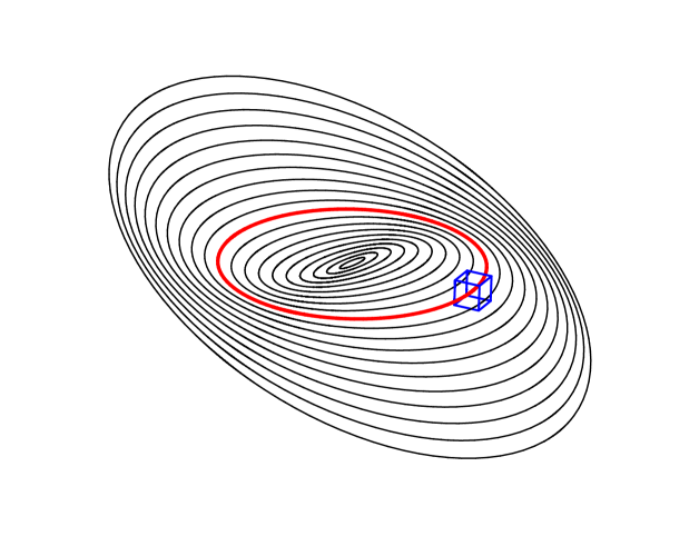
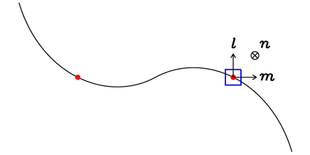
Figure 1: Top: Example of an untwisted warped disc, viewed as a collection of tilted rings. As discussed in Section 3, a reference orbit (red circle) is selected and used to construct a local Cartesian model of the disc. The local frame (blue box) is centred on a point that follows the reference orbit, and therefore experiences a geometry that oscillates at the orbital frequency as the local orientation of the midplane of the disc tilts back and forth. The illustrated box corresponds to the local frame at orbital phase $0$ according to our definitions, and its axes are aligned with the radius-dependent basis vectors $\{{\mn@boldsymbol{l}},{\mn@boldsymbol{m}},{\mn@boldsymbol{n}}\}$ at this phase only. In this example the warp amplitude at the reference radius is $|\psi|=0.5$. Bottom: Edge-on view of the warped disc, showing the local basis vectors.

The orbital angular velocity of the warped disc is ${\mn@boldsymbol{\Omega}}(r,t)=\Omega(r)\,{\mn@boldsymbol{l}}(r,t)$, where the slowly evolving unit tilt vector ${\mn@boldsymbol{l}}(r,t)$ is everywhere normal to the local orbital plane. The rate of orbital shear is

$${\mn@boldsymbol{S}}=r\frac{\partial{\mn@boldsymbol{\Omega}}}{\partial r}=r\frac{\mathrm{d}\Omega}{\mathrm{d}r}\,{\mn@boldsymbol{l}}+r\Omega\frac{\partial{\mn@boldsymbol{l}}}{\partial r}=-q\Omega\,{\mn@boldsymbol{l}}+|\psi|\Omega\,{\mn@boldsymbol{m}},$$ (1)

where $q=-\mathrm{d}\ln\Omega/\mathrm{d}\ln r$ is the usual dimensionless rate of orbital shear, equal to ${\textstyle\frac{3}{2}}$ for Keplerian orbits, $|\psi|=|\partial{\mn@boldsymbol{l}}/\partial\ln r|$ is the dimensionless warp amplitude defined by Ogilvie (1999), and ${\mn@boldsymbol{m}}$ is a unit vector parallel to $\partial{\mn@boldsymbol{l}}/\partial r$ and therefore orthogonal to ${\mn@boldsymbol{l}}$. A right-handed orthonormal triad $\{{\mn@boldsymbol{l}},{\mn@boldsymbol{m}},{\mn@boldsymbol{n}}\}$, dependent on $r$ and $t$ but not on the orbital phase, is completed by ${\mn@boldsymbol{n}}={\mn@boldsymbol{l}}\times{\mn@boldsymbol{m}}$ (Fig. 1, bottom). Note that none of these vectors is normal to the disc, in general.

The simplest type of warp is an ‘untwisted’ warp, by which we mean that, as in Fig. 1, the variation of the vectors ${\mn@boldsymbol{l}}$ and ${\mn@boldsymbol{m}}$ is confined to a plane, while the vector ${\mn@boldsymbol{n}}$ is perpendicular to that plane and independent of $r$. In the language of celestial mechanics, the longitude of the ascending node is independent of the semimajor axis. Although for clarity we choose untwisted warps for the purposes of illustration, our analysis is valid for general, twisted warps. Indeed, the parameter $|\psi|$ measures the local amplitude of the warp whether or not it is twisted. A local measure of twist would involve the second radial derivative of ${\mn@boldsymbol{l}}$, for example the triple scalar product of ${\mn@boldsymbol{l}}$, $\partial{\mn@boldsymbol{l}}/\partial\ln r$ and $\partial^{2}{\mn@boldsymbol{l}}/\partial(\ln r)^{2}$. (Some authors, however, have used the term ‘twisted disc’ as synonymous with ‘warped disc’.)

The significance of the parameter $|\psi|$ is illustrated in Fig. 2, where we present an edge-on view of discs with untwisted warps corresponding to different values of $|\psi|$. We will see in this paper and its companion that a warp of amplitude $|\psi|=0.01$, which might not be directly observable even with high-resolution imaging, can nevertheless have important dynamical consequences.

Figure 2: Edge-on view of discs with untwisted warps of constant amplitudes $|\psi|=0.01$ (top), $0.1$, $0.2$, $0.5$ and $1$ (bottom). Each curve is a logarithmic spiral.

The large-scale dynamics of a warped disc is governed by the conservation of mass and angular momentum (Papaloizou & Pringle, 1983; Pringle, 1992). The usual aim of a theory of warped discs is to obtain a system of partial differential equations in $r$ and $t$ that govern the shape and mass distribution of the disc. For a thin disc in which the angular momentum is dominated by orbital motion, the conservation laws in the absence of external influences can be written in the one-dimensional form

$$\frac{\partial\mathcal{M}}{\partial t}+\frac{\partial\mathcal{F}}{\partial r}=0,$$ (2)

$$\frac{\partial}{\partial t}(\mathcal{M}{\mn@boldsymbol{h}})+\frac{\partial}{\partial r}(\mathcal{F}{\mn@boldsymbol{h}}+{\mn@boldsymbol{\mathcal{G}}})=\mathbf{0},$$ (3)

where $\mathcal{M}(r,t)$ is the one-dimensional mass density of the disc (related to the surface density $\Sigma$ through $\mathcal{M}=2\pi r\Sigma$ and defined such that the mass contained between any two radii is given by an integral $\int\mathcal{M}\,\mathrm{d}r$ between those radii), $\mathcal{F}(r,t)$ is the outward radial flux of mass and ${\mn@boldsymbol{h}}(r,t)=r^{2}{\mn@boldsymbol{\Omega}}(r,t)=h(r){\mn@boldsymbol{l}}(r,t)$ is the specific angular momentum. The outward radial flux of angular momentum consists of two parts: $\mathcal{F}(r,t){\mn@boldsymbol{h}}(r,t)$ due to advection and ${\mn@boldsymbol{\mathcal{G}}}(r,t)$ being an internal torque associated with internal flows and stresses due to viscosity, magnetic fields, turbulence, self-gravitation, etc. Subtracting ${\mn@boldsymbol{h}}$ times equation (2) from equation (3), we obtain the equation governing the shape of the disc,

$$\mathcal{M}h\frac{\partial{\mn@boldsymbol{l}}}{\partial t}+\mathcal{F}\frac{\partial{\mn@boldsymbol{h}}}{\partial r}+\frac{\partial{\mn@boldsymbol{\mathcal{G}}}}{\partial r}=\mathbf{0}.$$ (4)

A scalar product with the unit vector ${\mn@boldsymbol{l}}$ gives

$$\mathcal{F}\frac{\mathrm{d}h}{\mathrm{d}r}+{\mn@boldsymbol{l}}\cdot\frac{\partial{\mn@boldsymbol{\mathcal{G}}}}{\partial r}=0,$$ (5)

which determines $\mathcal{F}$ in terms of ${\mn@boldsymbol{\mathcal{G}}}$. Therefore our task is to determine the internal torque ${\mn@boldsymbol{\mathcal{G}}}$. It is the transport of angular momentum that drives the evolution of both the shape of the disc and its mass distribution. The reason for this is of course that, within the family of circular orbits, the specific angular momentum vector determines both the orbital plane and the orbital radius.

This analysis is easily extended to allow for external forces by including a source term ${\mn@boldsymbol{\mathcal{T}}}$, the external torque per unit radius, on the right-hand side of equation (3).

Although the internal torque ${\mn@boldsymbol{\mathcal{G}}}$ at any radius in a thin disc involves an integral with respect to the azimuthal angle and is in this sense a global or large-scale quantity, we will see below that this integral naturally emerges in the form of a time-average in a local model that follows the orbital motion.

3 Local model of a warped disc

3.1 Geometry and particle dynamics

A local model can be constructed around any reference point that is situated on the warped midplane of the disc and moves in a circular orbit of radius $r_{0}$, where the orbital angular velocity is $\Omega_{0}=\Omega(r_{0})$. A Cartesian coordinate system is set up with its origin at the moving reference point and with axes that rotate with the orbital motion, so that the $x$, $y$ and $z$ directions are always radial, azimuthal and vertical. This is the standard construction of a local model, as used in the shearing sheet or shearing box.

The effective potential in this frame is the sum of the gravitational potential and the centrifugal potential arising from the rotation of the frame. When the effective potential is expanded in a Taylor series about the reference point and the unimportant constant term is neglected, the dominant terms are $-q\Omega_{0}^{2}x^{2}+{\textstyle\frac{1}{2}}\Omega_{0}^{2}z^{2}$. The equations of particle dynamics in this model are therefore

$$\ddot{x}-2\Omega_{0}\dot{y}=2q\Omega_{0}^{2}x,$$ (6)

$$\ddot{y}+2\Omega_{0}\dot{x}=0,$$ (7)

$$\ddot{z}=-\Omega_{0}^{2}z,$$ (8)

which reduce to Hill’s equations (without a satellite) in the Keplerian case $q={\textstyle\frac{3}{2}}$.

As stated above, we assume that the geometry of the warped disc can be regarded as fixed on the orbital time-scale relevant to the local model, although we discuss this assumption further in Section 4.4 below. The basis vectors associated with the warp at the reference radius, $\{{\mn@boldsymbol{l}}_{0},{\mn@boldsymbol{m}}_{0},{\mn@boldsymbol{n}}_{0}\}$, are therefore non-rotating, while the basis $\{{\mn@boldsymbol{e}}_{x},{\mn@boldsymbol{e}}_{y},{\mn@boldsymbol{e}}_{z}\}$ rotates as the reference point traverses its orbit. Without loss of generality, we choose the orbital phase of the reference point, or the origin of time, such that ${\mn@boldsymbol{m}}_{0}$ is in the radial direction at $t=0$ (as in Fig. 1). Then the basis vectors are related by

$${\mn@boldsymbol{l}}_{0}={\mn@boldsymbol{e}}_{z},\qquad{\mn@boldsymbol{m}}_{0}+\mathrm{i}{\mn@boldsymbol{n}}_{0}=({\mn@boldsymbol{e}}_{x}+\mathrm{i}{\mn@boldsymbol{e}}_{y})\mathrm{e}^{\mathrm{i}\Omega_{0}t}$$ (9)

(Fig. 3). While the rate of orbital shear is stationary in a non-rotating frame, in the local frame it rotates in a negative sense according to

$${\mn@boldsymbol{S}}_{0}(t)=-q\Omega_{0}\,{\mn@boldsymbol{e}}_{z}+|\psi|\Omega_{0}[{\mn@boldsymbol{e}}_{x}\cos(\Omega_{0}t)-{\mn@boldsymbol{e}}_{y}\sin(\Omega_{0}t)],$$ (10)

which follows from equations (1) and (9). In Fig. 1 the box can be thought of as following the red reference orbit, experiencing a local geometry that oscillates at the orbital frequency as the local orientation of the midplane of the disc tilts back and forth.

Figure 3: Time-dependent relation between the rotating horizontal basis vectors ${\mn@boldsymbol{e}}_{x}$ and ${\mn@boldsymbol{e}}_{y}$ of the local model and the non-rotating basis vectors ${\mn@boldsymbol{m}}_{0}$ and ${\mn@boldsymbol{n}}_{0}$ associated with the geometry of the warp at the reference radius. The vertical basis vectors ${\mn@boldsymbol{e}}_{z}$ and ${\mn@boldsymbol{l}}_{0}$ both point out of the page.

The local representation of circular orbital motion in the $xy$ plane is the linear motion $\dot{y}=-q\Omega_{0}x$ with $x=\mathrm{constant}$. To this can be added a free vertical oscillation $z=\mathrm{Re}(Z\,\mathrm{e}^{-\mathrm{i}\Omega_{0}t})$. The amplitude of the complex number $Z$ is related to the (small) inclination of the orbit with respect to the $xy$ plane, while the phase of $Z$ is related to the longitude of the ascending node; the complex tilt variable (used by Papaloizou & Pringle 1983 and many other authors), measured with respect to the $xy$ plane, would be $W=-Z/r_{0}$.

An orbital motion with a smooth warp can be represented locally by allowing $Z$ to vary linearly with $x$. Since the reference point is on the warped midplane of the disc, $Z$ vanishes at $x=0$. With the choice of orbital phase explained above, we have $Z=-|\psi|x$, and so $z=-|\psi|\cos(\Omega_{0}t)x$. This motion corresponds to the velocity field

$$\dot{\mn@boldsymbol{x}}={\mn@boldsymbol{u}}=-q\Omega_{0}x\,{\mn@boldsymbol{e}}_{y}+|\psi|\Omega_{0}\sin(\Omega_{0}t)x\,{\mn@boldsymbol{e}}_{z}.$$ (11)

Thus, while a particle at the origin remains there (corresponding to the reference orbit), a particle with a positive value of $x$ lags behind and also oscillates up and down at the orbital frequency (corresponding to an orbit slightly larger than the reference orbit).

Later we will need to calculate the internal torque in the local model. To prepare the way for this, we consider here the specific angular momentum, which in the local model can be regarded as

$$r_{0}(\dot{y}+2\Omega_{0}x){\mn@boldsymbol{e}}_{z}-r_{0}\dot{z}\,{\mn@boldsymbol{e}}_{y}-r_{0}\Omega_{0}z\,{\mn@boldsymbol{e}}_{x}.$$ (12)

The first two vectors involve non-radial motions combined with the long radial lever arm, while the third vector involves the large azimuthal motion combined with a vertical lever arm. (The $2\Omega_{0}x$ term represents the contribution to the azimuthal motion from the rotation of the frame of reference.) If we had also included the large azimuthal motion combined with the long radial lever arm, we would have obtained an additional term $r_{0}^{2}\Omega_{0}\,{\mn@boldsymbol{e}}_{z}={\mn@boldsymbol{h}}_{0}$, which is constant and large compared to the terms considered here. For a general particle motion governed by equations (6)–(8), it can be verified that the vector (12) is constant in a non-rotating frame. Its components in the local frame, however, are not constant.

For the orbital motion (11) associated with a warped disc, the specific angular momentum evaluates to

$$r_{0}({\mn@boldsymbol{S}}_{0}+2{\mn@boldsymbol{\Omega}}_{0})x=\left(\frac{\partial{\mn@boldsymbol{h}}}{\partial r}\right)_{0}x,$$ (13)

and therefore agrees with a linear local approximation to the orbital angular momentum. Again, if we had also included the large azimuthal motion combined with the long radial lever arm, we would have obtained an additional term ${\mn@boldsymbol{h}}_{0}$, which is constant and large compared to the terms considered here.

3.2 Fluid dynamics

So far we have considered the motion of test particles. The local hydrodynamic solutions for a warped disc are more complicated than the particle motion (11) because of pressure gradients. These solutions generally require numerical calculations and are most easily obtained by introducing a coordinate transformation that accounts for the warped orbital motion. Before doing so we establish the equations to be solved.

The basic equations for an ideal fluid in the local model (neglecting magnetic fields and self-gravity) are

$$\mathrm{D}u_{x}-2\Omega_{0}u_{y}=2q\Omega_{0}^{2}x-\frac{1}{\rho}\partial_{x}p,$$ (14)

$$\mathrm{D}u_{y}+2\Omega_{0}u_{x}=-\frac{1}{\rho}\partial_{y}p,$$ (15)

$$\mathrm{D}u_{z}=-\Omega_{0}^{2}z-\frac{1}{\rho}\partial_{z}p,$$ (16)

$$\mathrm{D}\rho=-\rho(\partial_{x}u_{x}+\partial_{y}u_{y}+\partial_{z}u_{z}),$$ (17)

where

$$\mathrm{D}=\partial_{t}+u_{x}\partial_{x}+u_{y}\partial_{y}+u_{z}\partial_{z}$$ (18)

is the Lagrangian derivative, ${\mn@boldsymbol{u}}$ is the velocity, $\rho$ is the density and $p$ is the pressure. These are the standard equations for hydrodynamics in the shearing sheet or box (e.g. Hawley, Gammie & Balbus, 1995). For simplicity, we consider an isothermal gas for which

$$p=c_{\mathrm{s}}^{2}\rho,$$ (19)

where $c_{\mathrm{s}}=\mathrm{constant}$ is the isothermal sound speed. In terms of the pseudo-enthalpy

$$h=c_{\mathrm{s}}^{2}\ln\rho+\mathrm{constant},$$ (20)

we then have

$$\mathrm{D}u_{x}-2\Omega_{0}u_{y}=2q\Omega_{0}^{2}x-\partial_{x}h,$$ (21)

$$\mathrm{D}u_{y}+2\Omega_{0}u_{x}=-\partial_{y}h,$$ (22)

$$\mathrm{D}u_{z}=-\Omega_{0}^{2}z-\partial_{z}h,$$ (23)

$$\mathrm{D}h=-c_{\mathrm{s}}^{2}(\partial_{x}u_{x}+\partial_{y}u_{y}+\partial_{z}u_{z}).$$ (24)

The alternative equations for adiabatic flow are developed in Appendix A.

Note that our local model correctly includes the vertical gravitational acceleration $-\Omega_{0}^{2}z$ deriving from a spherically symmetric potential. Without this term the model would be incapable of representing a warped disc and the dynamics described in this paper would not occur.

If the disc is unwarped, the orbital plane everywhere coincides with the $xy$ plane and the local representation of circular orbital motion is ${\mn@boldsymbol{u}}=-q\Omega_{0}x\,{\mn@boldsymbol{e}}_{y}$. Equations (21)–(24) are then satisfied when hydrostatic equilibrium, $\partial_{z}h=-\Omega_{0}^{2}z$, is also imposed.

If the disc is warped at the reference radius, then we might expect the velocity field (11) corresponding to the warped orbital motion to satisfy the hydrodynamic equations (21)–(24), together with some version of hydrostatic equilibrium. However, this is not the case; the problem lies with equation (23). If hydrostatic equilibrium, $\partial_{z}h=-\Omega_{0}^{2}z$, is imposed, then there is an unbalanced, $x$-dependent acceleration on the left-hand side of equation (23). If the pressure is allowed to vary with $x$ to compensate for this term, then equation (21) is disrupted. The actual hydrodynamic solutions must be more complicated than equation (11) in order to account for the interplay of these additional forces. The simplest (laminar) versions of these solutions are derived in Section 4 below.

3.3 Warped shearing coordinates

We now adapt the local model to incorporate the oscillating local geometry of the warp explicitly. This will allow us to find the simplest hydrodynamic states and to formulate a theoretical and computational model for the further study of warped discs.

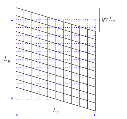
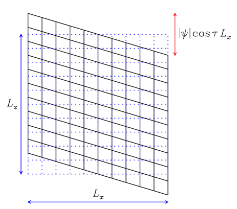
Figure 4: Illustration of warped shearing coordinates. The dotted blue grid represents the Cartesian coordinates of the standard local approximation or shearing box, while the solid black grid represents the warped shearing coordinates. The shear in the $xy$ plane (left) increases linearly with time, although in a computational model the grid should be remapped periodically by resetting the origin of time. The shear in the $xz$ plane (right) oscillates at the orbital frequency and is proportional to the amplitude of the warp.

We introduce new coordinates

$$t^{\prime}=t,$$ (25)

$$x^{\prime}=x,$$ (26)

$$y^{\prime}=y+q\Omega_{0}tx,$$ (27)

$$z^{\prime}=z+|\psi|\cos(\Omega_{0}t)x$$ (28)

that follow the warped orbital motion: a particle on an inclined circular orbit would have constant $x^{\prime}$, $y^{\prime}$ and $z^{\prime}$. We define the orbital phase

$$\tau=\Omega_{0}t^{\prime}=\Omega_{0}t.$$ (29)

Partial derivatives transform according to

$$\partial_{t}=\partial_{t}^{\prime}+q\Omega_{0}x\partial_{y}^{\prime}-|\psi|\Omega_{0}\sin\tau\,x\partial_{z}^{\prime},$$ (30)

$$\partial_{x}=\partial_{x}^{\prime}+q\tau\,\partial_{y}^{\prime}+|\psi|\cos\tau\,\partial_{z}^{\prime},$$ (31)

$$\partial_{y}=\partial_{y}^{\prime},$$ (32)

$$\partial_{z}=\partial_{z}^{\prime},$$ (33)

so that

$$\mathrm{D}=\partial_{t}^{\prime}+v_{x}\partial_{x}^{\prime}+(v_{y}+q\tau v_{x})\partial_{y}^{\prime}+(v_{z}+|\psi|\cos\tau\,v_{x})\partial_{z}^{\prime},$$ (34)

where

$$v_{x}=u_{x},$$ (35)

$$v_{y}=u_{y}+q\Omega_{0}x,$$ (36)

$$v_{z}=u_{z}-|\psi|\Omega_{0}\sin\tau\,x$$ (37)

are the relative velocity components. Thus, if ${\mn@boldsymbol{v}}=\mathbf{0}$ (which is not a solution of the equations), the fluid follows the prescribed warped orbital motion and the velocity ${\mn@boldsymbol{u}}$, which corresponds to the rate of change of the Cartesian coordinates $(x,y,z)$, is non-zero. (We should not call ${\mn@boldsymbol{u}}$ the absolute velocity, however, because it is measured in a rotating frame of reference.) We continue to refer vector components to the Cartesian basis $\{{\mn@boldsymbol{e}}_{x},{\mn@boldsymbol{e}}_{y},{\mn@boldsymbol{e}}_{z}\}$. The grid of warped shearing coordinates is illustrated in Fig. 4.

The hydrodynamic equations are therefore transformed into

$$\mathrm{D}v_{x}-2\Omega_{0}v_{y}=-(\partial_{x}^{\prime}+q\tau\,\partial_{y}^{\prime}+|\psi|\cos\tau\,\partial_{z}^{\prime})h,$$ (38)

$$\mathrm{D}v_{y}+(2-q)\Omega_{0}v_{x}=-\partial_{y}^{\prime}h,$$ (39)

$$\mathrm{D}v_{z}+|\psi|\Omega_{0}\sin\tau\,v_{x}=-\Omega_{0}^{2}z^{\prime}-\partial_{z}^{\prime}h,$$ (40)

$$\mathrm{D}h=-c_{\mathrm{s}}^{2}[(\partial_{x}^{\prime}+q\tau\,\partial_{y}^{\prime}+|\psi|\cos\tau\,\partial_{z}^{\prime})v_{x}+\partial_{y}^{\prime}v_{y}+\partial_{z}^{\prime}v_{z}].$$ (41)

An alternative form of equation (41), in which the conservation of mass is manifest, is

$$\partial_{t}^{\prime}\rho+\partial_{x}^{\prime}(\rho v_{x})+\partial_{y}^{\prime}[\rho(v_{y}+q\tau v_{x})]$$ (42)

$$+\partial_{z}^{\prime}[\rho(v_{z}+|\psi|\cos\tau\,v_{x})]=0.$$

These equations contain $\tau$ explicitly but not $x^{\prime}$ or $y^{\prime}$. This shows that the local model of a warped disc is horizontally homogeneous. As in the standard shearing sheet, every point in the $x^{\prime}y^{\prime}$ plane is equivalent, if allowance is made for an appropriate change of frame of reference.

We can see from these equations that ${\mn@boldsymbol{v}}=\mathbf{0}$ is not a solution in the presence of a warp. Equation (40) would require hydrostatic equilibrium in the form $\partial_{z}^{\prime}h=-\Omega_{0}^{2}z^{\prime}$, but this would provide an unbalanced horizontal force in equation (38), as illustrated in Fig. 5.

Figure 5: Regions of high (H) and low (L) pressure in the local representation of a warped disc, showing how the hydrostatic vertical pressure gradient leads to a horizontal force that is unbalanced by gravity (arrows). The $xz$ plane (of unwarped coordinates) is depicted at $t=0$, with the dotted line corresponding to $z=0$. These horizontal pressure gradients oscillate at the orbital frequency as the local geometry tilts back and forth, giving rise to oscillatory planar motions.

The total energy equation associated with equations (38)–(41) is

$$\partial_{t}^{\prime}(\rho\mathcal{E})+\partial_{x}^{\prime}[(\rho\mathcal{E}+p)v_{x}]+\partial_{y}^{\prime}[(\rho\mathcal{E}+p)(v_{y}+q\tau v_{x})]$$ (43)

$$+\partial_{z}^{\prime}[(\rho\mathcal{E}+p)(v_{z}+|\psi|\cos\tau\,v_{x})]$$

$$=\rho v_{x}(q\Omega_{0}v_{y}-|\psi|\Omega_{0}\sin\tau\,v_{z}+|\psi|\Omega_{0}\cos\tau\,\Omega_{0}z^{\prime}),$$

where

$$\mathcal{E}=\frac{1}{2}(v_{x}^{2}+v_{y}^{2}+v_{z}^{2})+h+\frac{1}{2}\Omega_{0}^{2}z^{\prime 2}.$$ (44)

We will interpret the source term on the right-hand side of equation (43) below.

3.4 Fluxes of mass and angular momentum

In order to connect the local model with the large-scale dynamics of the warped disc described in Section 2, we consider the outward radial fluxes of mass and angular momentum. The mass flux at the reference radius $r_{0}$ is

$$\mathcal{F}_{0}=\int\!\!\int_{0}^{2\pi}\langle\rho u_{x}\rangle_{\mathrm{h}}\,r_{0}\,\mathrm{d}\tau\,\mathrm{d}z^{\prime}$$ (45)

(in which $u_{x}$ can be replaced by $v_{x}$), where the notation $\langle\cdot\rangle_{\mathrm{h}}$ denotes local horizontal averaging over the coordinates $x^{\prime}$ and $y^{\prime}$ (where necessary), and the $z^{\prime}$ integral is over the entire vertical extent of the disc. The $\tau$ integral, which in the local model is with respect to time, can be interpreted as an integral with respect to azimuth as the reference point traverses its orbit. Similarly, the angular-momentum flux in the local model is (cf. equations 12 and 13)

$$\mathcal{F}_{0}\left(\frac{\partial{\mn@boldsymbol{h}}}{\partial r}\right)_{0}x+{\mn@boldsymbol{\mathcal{G}}}_{0}=\int\!\!\int_{0}^{2\pi}\big{\langle}\rho u_{x}[r_{0}(u_{y}+2\Omega_{0}x)\,{\mn@boldsymbol{e}}_{z}-r_{0}u_{z}\,{\mn@boldsymbol{e}}_{y}$$ (46)

$$\qquad\qquad\qquad\qquad\qquad-r_{0}\Omega_{0}z\,{\mn@boldsymbol{e}}_{x}]\big{\rangle}_{\mathrm{h}}\,r_{0}\,\mathrm{d}\tau\,\mathrm{d}z^{\prime}.$$

As in equation (12), the first two vectors inside the square brackets, contributing to the specific angular momentum of the fluid, involve non-radial motions combined with the long radial lever arm, while the third expression involves the large azimuthal motion combined with a vertical lever arm; again, we choose not to include the larger constant term involving the large azimuthal motion combined with the long radial lever arm, which generates the larger flux $\mathcal{F}_{0}{\mn@boldsymbol{h}}_{0}$. Writing ${\mn@boldsymbol{u}}$ and $z$ in terms of ${\mn@boldsymbol{v}}$ and $z^{\prime}$, and using the definition (45) of $\mathcal{F}_{0}$, we find that the terms proportional to $x$ on each side of the equation cancel, leaving

$${\mn@boldsymbol{\mathcal{G}}}_{0}=\int\!\!\int_{0}^{2\pi}\langle{\mn@boldsymbol{g}}_{0}\rangle_{\mathrm{h}}\,r_{0}\,\mathrm{d}\tau\,\mathrm{d}z^{\prime},$$ (47)

where

$${\mn@boldsymbol{g}}_{0}=\rho v_{x}(r_{0}v_{y}\,{\mn@boldsymbol{e}}_{z}-r_{0}v_{z}\,{\mn@boldsymbol{e}}_{y}-r_{0}\Omega_{0}z^{\prime}\,{\mn@boldsymbol{e}}_{x})$$ (48)

is the internal torque per unit area. We then recognize the right-hand side of equation (43) as the scalar product $-({\mn@boldsymbol{g}}_{0}\cdot{\mn@boldsymbol{S}}_{0})/r_{0}$, which is the rate at which energy is extracted, per unit volume, by the torque acting on the orbital shear.

So far we have considered inviscid hydrodynamics. More generally, there may be shear stresses in the fluid resulting from viscosity or magnetic fields. In the presence of a symmetric stress tensor $\mathbf{T}$, which can also represent the effects of turbulence or self-gravitation, the torque per unit area is given by the more general expression

$$\frac{{\mn@boldsymbol{g}}_{0}}{r_{0}}=\rho v_{x}(v_{y}\,{\mn@boldsymbol{e}}_{z}-v_{z}\,{\mn@boldsymbol{e}}_{y}-\Omega_{0}z^{\prime}\,{\mn@boldsymbol{e}}_{x})-T_{xy}\,{\mn@boldsymbol{e}}_{z}+T_{xz}\,{\mn@boldsymbol{e}}_{y}.$$ (49)

In the case of a viscous stress, for example,

$$T_{xy}=\mu[-q\Omega_{0}+(\partial_{x}^{\prime}+q\tau\,\partial_{y}^{\prime}+|\psi|\cos\tau\,\partial_{z}^{\prime})v_{y}+\partial_{y}^{\prime}v_{x}]$$ (50)

and

$$T_{xz}=\mu[|\psi|\Omega_{0}\sin\tau+(\partial_{x}^{\prime}+q\tau\,\partial_{y}^{\prime}+|\psi|\cos\tau\,\partial_{z}^{\prime})v_{z}+\partial_{z}^{\prime}v_{x}]$$ (51)

are the relevant components, where $\mu$ is the dynamic viscosity.

Since ${\mn@boldsymbol{g}}_{0}\cdot{\mn@boldsymbol{l}}_{0}=g_{0z}$, the vertical component of the torque is given by

$$\frac{{\mn@boldsymbol{\mathcal{G}}}_{0}\cdot{\mn@boldsymbol{l}}_{0}}{2\pi r_{0}^{2}}=\bigg{\langle}\int(\rho v_{x}v_{y}-T_{xy})\,\mathrm{d}z^{\prime}\bigg{\rangle}_{\!\!\mathrm{h},\tau},$$ (52)

where the notation $\langle\cdot\rangle_{\mathrm{h},\tau}$ denotes horizontal averaging over the coordinates $x^{\prime}$ and $y^{\prime}$ (where necessary) and averaging over the orbital phase $\tau$. This is easily understood as involving the radial transport of azimuthal momentum (or vertical angular momentum) by Reynolds and viscous (or other) stresses.

In computing the horizontal components of the torque we must bear in mind that the basis vectors ${\mn@boldsymbol{e}}_{x}$ and ${\mn@boldsymbol{e}}_{y}$ depend on orbital phase. We make use of a complex notation and equation (9). Thus

$${\mn@boldsymbol{g}}_{0}\cdot({\mn@boldsymbol{m}}_{0}+\mathrm{i}{\mn@boldsymbol{n}}_{0})=(g_{0x}+\mathrm{i}g_{0y})\mathrm{e}^{\mathrm{i}\tau}$$ (53)

and so

$$\frac{{\mn@boldsymbol{\mathcal{G}}}_{0}\cdot({\mn@boldsymbol{m}}_{0}+\mathrm{i}{\mn@boldsymbol{n}}_{0})}{2\pi r_{0}^{2}}=$$ (54)

$$\qquad\bigg{\langle}\mathrm{e}^{\mathrm{i}\tau}\int[\rho v_{x}(-\Omega_{0}z^{\prime}-\mathrm{i}v_{z})+\mathrm{i}T_{xz}]\,\mathrm{d}z^{\prime}\bigg{\rangle}_{\!\!\mathrm{h},\tau}.$$

The horizontal components of the torque are conveniently encoded in the real and imaginary parts of this expression. Not surprisingly, it involves the radial transport of vertical momentum (or horizontal angular momentum).

It is natural to represent the torque for an isothermal disc in the form (cf. Ogilvie, 1999)

$${\mn@boldsymbol{\mathcal{G}}} = -2\pi\Sigma c_{\mathrm{s}}^{2}r^{2}(Q_{1}\,{\mn@boldsymbol{l}}+Q_{2}|\psi|\,{\mn@boldsymbol{m}}+Q_{3}|\psi|\,{\mn@boldsymbol{n}})$$ (55)

$$= -2\pi\Sigma c_{\mathrm{s}}^{2}r^{2}\left(Q_{1}\,{\mn@boldsymbol{l}}+Q_{2}r\frac{\partial{\mn@boldsymbol{l}}}{\partial r}+Q_{3}r\,{\mn@boldsymbol{l}}\times\frac{\partial{\mn@boldsymbol{l}}}{\partial r}\right),$$

where $Q_{1}$, $Q_{2}$ and $Q_{3}$ are dimensionless coefficients and

$$\Sigma=\bigg{\langle}\int\rho\,\mathrm{d}z^{\prime}\bigg{\rangle}_{\!\!\mathrm{h}}$$ (56)

is the horizontally averaged surface density of the disc, which is independent of $\tau$ by virtue of mass conservation. This representation is just a projection of the torque on to the local basis defined by the geometry of the disc. Comparison of the vertical component of the torque shows that

$$-Q_{1}\Sigma c_{\mathrm{s}}^{2}=\bigg{\langle}\int(\rho v_{x}v_{y}-T_{xy})\,\mathrm{d}z^{\prime}\bigg{\rangle}_{\!\!\mathrm{h},\tau},$$ (57)

while comparison of the horizontal components shows that

$$-Q_{4}|\psi|\Sigma c_{\mathrm{s}}^{2}=\bigg{\langle}\mathrm{e}^{\mathrm{i}\tau}\int[\rho v_{x}(-\Omega_{0}z^{\prime}-\mathrm{i}v_{z})+\mathrm{i}T_{xz}]\,\mathrm{d}z^{\prime}\bigg{\rangle}_{\!\!\mathrm{h},\tau},$$ (58)

where $Q_{4}=Q_{2}+\mathrm{i}Q_{3}$ is a useful combination. Roughly speaking, the $Q_{1}$ term is similar to the usual torque in an accretion disc, and (if negative) causes the mass distribution to evolve diffusively, while the $Q_{2}$ term (if positive) causes a diffusion of the warp and the $Q_{3}$ term causes a dispersive wavelike propagation of the warp.

The correspondence between these dimensionless torque coefficients and the viscosity coefficients $\nu_{1}$ and $\nu_{2}$ of Pringle (1992) (deriving from the ‘naive approach’ in Section 2 of Papaloizou & Pringle 1983) is

$$Q_{1}c_{\mathrm{s}}^{2}=-q\nu_{1}\Omega,\qquad Q_{2}c_{\mathrm{s}}^{2}={\textstyle\frac{1}{2}}\nu_{2}\Omega,$$ (59)

while $Q_{3}$ has no counterpart in that description. (It would be potentially misleading to associate $Q_{3}$ with a ‘viscosity’ coefficient $\nu_{3}$ because the $Q_{3}$ term is non-dissipative. However, the combination $Q_{4}=Q_{2}+\mathrm{i}Q_{3}$ does emerge naturally as a complex diffusion coefficient, especially in linear theory.)

Since the shape of the disc is defined in the local model only by the dimensionless warp amplitude $|\psi|$, it is natural to expect the dimensionless torque coefficients $Q_{1}$, $Q_{2}$ and $Q_{3}$ to emerge as functions of $|\psi|$, as well as any other relevant dimensionless parameters such as $\alpha$. We will see in Section 4.5 how this works for laminar flows, but in the presence of instability and turbulence these functions must be determined by means of numerical simulations.

3.5 Computational considerations

The hydrodynamic equations (38)–(41) or their equivalents can be solved numerically by standard methods, for example by using finite differences on a regular grid in the coordinates $(x^{\prime},y^{\prime},z^{\prime})$ and imposing periodic boundary conditions in $x^{\prime}$ and $y^{\prime}$ and some other appropriate boundary conditions in $z^{\prime}$. The additional terms proportional to $|\psi|$ would of course require some rewriting of existing codes. Note that the primed coordinate grid undergoes an inexorable shearing, even in the absence of a warp. The coordinates should therefore be remapped periodically to avoid excessive distortion of the grid. This procedure is equivalent to periodically resetting the arbitrary origin of time, and can be done without interpolation if the remapping frequency and the aspect ratio of the grid are chosen correctly. In the case of a warped disc with its oscillating local geometry, it may be convenient to remap once per orbital period, for example by letting $\tau$ run from $-\pi$ to $\pi$ repeatedly, giving rise to a periodic dynamical system.

In the standard shearing box for an unwarped disc, there are in fact two different methods of solving the hydrodynamic equations. The more common method is to discretize the equations (with time-independent coefficients) in a cuboidal domain in unsheared coordinates $(x,y,z)$ and to apply (time-dependent) modified periodic boundary conditions. The other method is to discretize the equations (with time-dependent coefficients) in a cuboidal domain in sheared coordinates $(x^{\prime},y^{\prime},z^{\prime})$ (with periodic remapping of the grid) and to apply (time-independent) periodic boundary conditions. For a warped disc, only the second approach is possible: the equations must be discretized in primed coordinates, because a fixed cuboidal domain in unprimed coordinates cannot represent the regions above and below the warped midplane of the disc in a way that allows the radial boundaries to be identified (cf. Fig. 5). This limitation is related to the fact that vertical gravity is essential to the description of a warped disc, and the $z$ direction cannot be regarded as periodic. When supplied with periodic boundary conditions in $x^{\prime}$ and $y^{\prime}$, our local model takes the form of a warped shearing box.

4 Laminar flows

4.1 Separation of variables

The simplest solutions of equations (38)–(41) are in fact independent of $x^{\prime}$ and $y^{\prime}$ and $2\pi$-periodic in $\tau$: they are horizontally uniform and oscillate at the orbital frequency. (In a global context, such local solutions correspond to the situation in which the warped disc has a structure that varies on a horizontal length-scale much larger than the thickness of the disc, and on a time-scale much longer than the orbital time-scale.) These laminar flows satisfy

$$\mathrm{D}v_{x}-2\Omega_{0}v_{y}=-|\psi|\cos\tau\,\partial_{z}^{\prime}h,$$ (60)

$$\mathrm{D}v_{y}+(2-q)\Omega_{0}v_{x}=0,$$ (61)

$$\mathrm{D}v_{z}+|\psi|\Omega_{0}\sin\tau\,v_{x}=-\Omega_{0}^{2}z^{\prime}-\partial_{z}^{\prime}h,$$ (62)

$$\mathrm{D}h=-c_{\mathrm{s}}^{2}(|\psi|\cos\tau\,\partial_{z}^{\prime}v_{x}+\partial_{z}^{\prime}v_{z}),$$ (63)

with

$$\mathrm{D}=\partial_{t}^{\prime}+(v_{z}+|\psi|\cos\tau\,v_{x})\partial_{z}^{\prime}.$$ (64)

A nonlinear separation of variables is then possible, with

$$v_{x}(z^{\prime},t^{\prime})=u(\tau)\Omega_{0}z^{\prime},$$ (65)

$$v_{y}(z^{\prime},t^{\prime})=v(\tau)\Omega_{0}z^{\prime},$$ (66)

$$v_{z}(z^{\prime},t^{\prime})=w(\tau)\Omega_{0}z^{\prime},$$ (67)

$$h(z^{\prime},t^{\prime})=c_{\mathrm{s}}^{2}f(\tau)-{\textstyle\frac{1}{2}}\Omega_{0}^{2}z^{\prime 2}g(\tau),$$ (68)

where $u$, $v$, $w$, $f$ and $g$ are all dimensionless. Thus

$$\mathrm{d}_{\tau}u+(w+|\psi|\cos\tau\,u)u-2v=|\psi|\cos\tau\,g,$$ (69)

$$\mathrm{d}_{\tau}v+(w+|\psi|\cos\tau\,u)v+(2-q)u=0,$$ (70)

$$\mathrm{d}_{\tau}w+(w+|\psi|\cos\tau\,u)w+|\psi|\sin\tau\,u=g-1,$$ (71)

$$\mathrm{d}_{\tau}f=-(w+|\psi|\cos\tau\,u),$$ (72)

$$\mathrm{d}_{\tau}g=-2(w+|\psi|\cos\tau\,u)g,$$ (73)

where $\mathrm{d}_{\tau}$ denotes the ordinary derivative $\mathrm{d}/\mathrm{d}\tau$.

When a dynamic shear viscosity $\mu=\alpha p/\Omega_{0}$ and a dynamic bulk viscosity $\mu_{\mathrm{b}}=\alpha_{\mathrm{b}}p/\Omega_{0}$ are included, where $\alpha$ and $\alpha_{\mathrm{b}}$ are constant dimensionless coefficients (thus providing a kinematic shear viscosity $\nu=\alpha c_{\mathrm{s}}^{2}/\Omega_{0}$, etc.), these equations become

$$\mathrm{d}_{\tau}u+(w+|\psi|\cos\tau\,u)u-2v=|\psi|\cos\tau\,g$$ (74)

$$-(\alpha_{\mathrm{b}}+{\textstyle\frac{1}{3}}\alpha)|\psi|\cos\tau\,g(w+|\psi|\cos\tau\,u)$$

$$-\alpha g[|\psi|\sin\tau+(1+|\psi|^{2}\cos^{2}\tau)u],$$

$$\mathrm{d}_{\tau}v+(w+|\psi|\cos\tau\,u)v+(2-q)u$$ (75)

$$=-\alpha g[-q|\psi|\cos\tau+(1+|\psi|^{2}\cos^{2}\tau)v],$$

$$\mathrm{d}_{\tau}w+(w+|\psi|\cos\tau\,u)w+|\psi|\sin\tau\,u=g-1$$ (76)

$$-(\alpha_{\mathrm{b}}+{\textstyle\frac{1}{3}}\alpha)g(w+|\psi|\cos\tau\,u)$$

$$-\alpha g[|\psi|^{2}\sin\tau\cos\tau+(1+|\psi|^{2}\cos^{2}\tau)w],$$

$$\mathrm{d}_{\tau}f=-(w+|\psi|\cos\tau\,u),$$ (77)

$$\mathrm{d}_{\tau}g=-2(w+|\psi|\cos\tau\,u)g.$$ (78)

Our numerical treatment of these ordinary differential equations in Section 4.3 below provides us with a family of ‘exact’ nonlinear solutions representing the laminar flows in a warped disc. The same laminar flows, combined with the warping motion, can alternatively be regarded as nonlinear solutions of equations (21)–(24) in the variables of the standard shearing sheet, although they do not then appear to be horizontally uniform and it would not be obvious how to obtain them without making the transformation to warped coordinates. For example, the vertical velocity would be

$$u_{z}=|\psi|\Omega_{0}\sin\tau\,x+w(\tau)\Omega_{0}(z+|\psi|\cos\tau\,x).$$ (79)

The differential equations for $f$ and $g$ are related in such a way that the surface density of the disc, which is proportional to $\mathrm{e}^{f}g^{-1/2}$, is independent of $\tau$. The total energy equation for the laminar flows has the form

$$\mathrm{d}_{\tau}\left[\frac{1}{2g}(u^{2}+v^{2}+w^{2}+g\ln g+1)\right]$$ (80)

$$=\frac{1}{g}(quv-|\psi|\sin\tau\,uw+|\psi|\cos\tau\,u)$$

$$-\alpha|\psi|(\sin\tau\,u-q\cos\tau\,v+|\psi|\sin\tau\cos\tau\,w)$$

$$-\alpha(1+|\psi|^{2}\cos^{2}\tau)(u^{2}+v^{2}+w^{2})$$

$$-(\alpha_{\mathrm{b}}+{\textstyle\frac{1}{3}}\alpha)(w+|\psi|\cos\tau\,u)^{2}.$$

The first expression on the right-hand side is equivalent to the right-hand side of equation (43) and corresponds to the extraction of energy by the torque acting on the orbital shear. The third and fourth expressions are negative definite and correspond to viscous damping of the flow. The second expression is proportional to viscosity but is not negative definite; its interpretation is not straightforward.

In Appendix A we give the corresponding equations for adiabatic flow. They are exactly equivalent to those derived by Ogilvie (1999) in a different way, by writing the hydrodynamic equations in a warped spherical polar coordinate system that follows the global distortion of the warped midplane, and carrying out an asymptotic expansion of the solution in the limit of a thin disc. In that paper the orbital phase $\tau$ is directly related to the azimuthal angle $\phi$. Here we have not explicitly made use of an asymptotic expansion, but have derived the equations consistently within the context of the local approximation.

4.2 Horizontal and vertical oscillators

The physical interpretation of the laminar flows is assisted by changing to the variables

$$(U,V,W)=(u,v,w)H,\qquad H=g^{-1/2}.$$ (81)

Since the density and pressure then have the form

$$\rho\propto p\propto\exp\left\{f(\tau)-\frac{1}{2}\left[\frac{\Omega_{0}z^{\prime}}{c_{\mathrm{s}}H(\tau)}\right]^{2}\right\},$$ (82)

it can be seen that $H(\tau)$ is the scale-height of the disc in units of the scale-height $c_{\mathrm{s}}/\Omega_{0}$ of an equilibrium unwarped disc. The variables $(U,V,W)$ are therefore more like momenta, or vertically integrated velocities.

In the inviscid case we then have

$$\mathrm{d}_{\tau}U-2V=|\psi|\cos\tau\,H^{-1},$$ (83)

$$\mathrm{d}_{\tau}V+(2-q)U=0,$$ (84)

$$\mathrm{d}_{\tau}W+|\psi|\sin\tau\,U=H^{-1}-H,$$ (85)

$$\mathrm{d}_{\tau}H=W+|\psi|\cos\tau\,U.$$ (86)

In the absence of a warp ($|\psi|=0$), equations (83) and (84) describe a linear epicyclic oscillator. They can be combined to give $\mathrm{d}_{\tau}^{2}V=-2(2-q)V$, or the same equation for $U$. Equations (85) and (86) describe a nonlinear vertical oscillator, the ‘breathing mode’ of the disc. They can be combined to give $\mathrm{d}_{\tau}^{2}H=H^{-1}-H$. The vertical oscillator therefore has a potential energy function $-\ln H+{\textstyle\frac{1}{2}}H^{2}+\mathrm{constant}$, representing the sum of internal energy and gravitational energy, with equilibrium at $H=1$. It can in principle support oscillations of any energy, but this may involve severe compression because of the slow divergence of the potential as $H\to 0$. The natural frequency of the oscillator in the linear regime is $\sqrt{2}\,\Omega_{0}$ (or $\sqrt{\gamma+1}\,\Omega_{0}$ for an arbitrary adiabatic exponent $\gamma$); more generally, it depends on the amplitude of the oscillation.

The horizontal and vertical oscillators are coupled in the presence of a warp. The $|\psi|$ term in equation (83) represents the radial pressure gradient that occurs in a warped disc: in the absence of a warp, the pressure varies with $z$ to provide hydrostatic equilibrium, and warping of the disc causes a radial gradient to appear (Fig. 5). The $|\psi|$ term in equation (85) represents the horizontal transport of the vertical momentum of the warped orbital motion. Finally, the $|\psi|$ term in equation (86) represents a contribution to the velocity divergence from horizontal motion in a warped disc. These coupled horizontal and vertical oscillators featured prominently in the analysis of weakly nonlinear bending waves in Keplerian discs by Ogilvie (2006).

As we have seen, the viscous terms in a warped disc have a complicated form. In the absence of a warp, the equations for laminar viscous flows can be written

$$\mathrm{d}_{\tau}U-2V=-\alpha H^{-2}U,$$ (87)

$$\mathrm{d}_{\tau}V+(2-q)U=-\alpha H^{-2}V,$$ (88)

$$\mathrm{d}_{\tau}W=H^{-1}-H-(\alpha_{\mathrm{b}}+{\textstyle\frac{4}{3}}\alpha)H^{-2}W,$$ (89)

$$\mathrm{d}_{\tau}H=W,$$ (90)

showing that the horizontal motion is damped by shear viscosity while the vertical motion is damped by both shear and bulk viscosity.

4.3 Numerical solutions

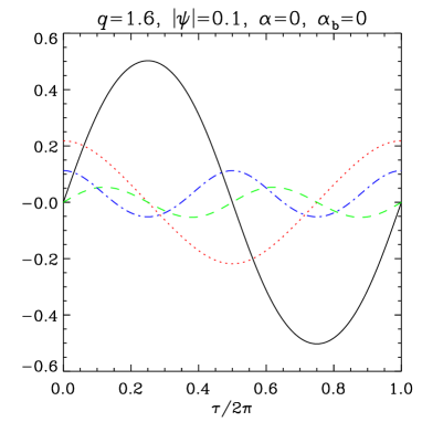
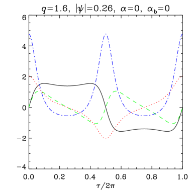
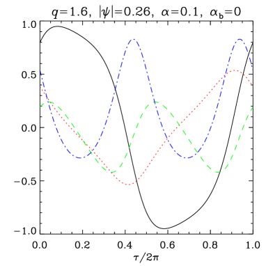
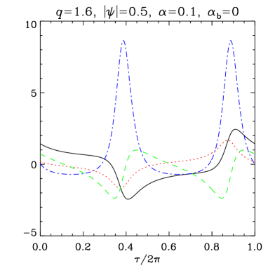
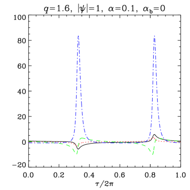
Figure 6: Selection of laminar flows for $q=1.6$. Solid (black), dotted (red), dashed (green) and dot-dashed (blue) lines represent $u$, $v$, $w$ and $g-1$, respectively (see equations 65–68). The inviscid solutions terminate at $|\psi|\approx 0.261$ in this case, but larger values of $|\psi|$ can be reached by including viscosity.

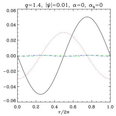
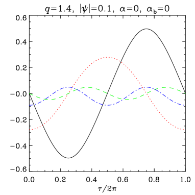
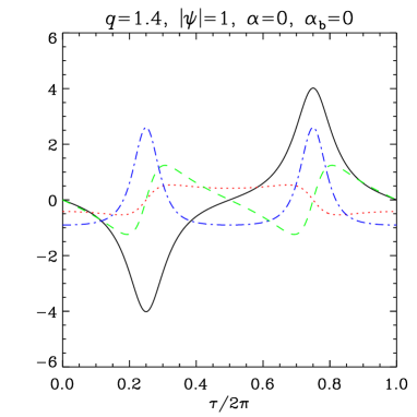
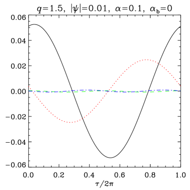
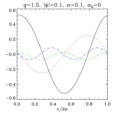
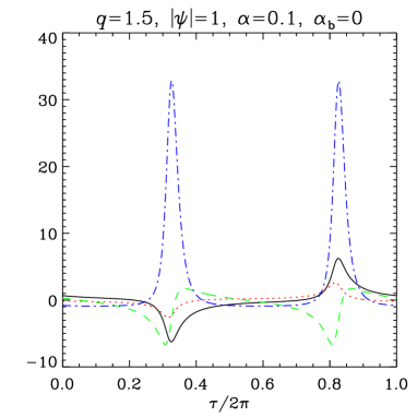
Figure 7: Continuation of Fig. 6 for $q=1.4$ and $q=1.5$. The inviscid solutions for $q=1.4$ continue to large values of $|\psi|$. For $q=1.5$ some viscosity is required.

Typical numerical solutions for the laminar flows are shown in Figs 6 and 7. These were computed by a standard shooting method using a Runge–Kutta integrator with adaptive stepsize. We first consider the inviscid case $\alpha=\alpha_{\mathrm{b}}=0$ for a non-Keplerian disc with $q=1.6$ (Fig. 6, panels 1–3). Note that the regime ${\textstyle\frac{3}{2}}<q<2$, in which the epicyclic frequency is positive but less than the orbital frequency, corresponds to conditions close to a black hole, where relativistic effects are important. For sufficiently small warp amplitude $|\psi|$, the horizontal flows $u$ and $v$ are proportional to $|\psi|$ and have a sinusoidal dependence on orbital phase, corresponding to the linear horizontal oscillator being driven at the orbital frequency, which here is greater than the natural (epicyclic) frequency of the oscillator (panels 1–2). The vertical velocity $w$ and the departure from hydrostatic equilibrium, $g-1$, are proportional to $|\psi|^{2}$ and therefore smaller. (Note that $w$ does not include the vertical velocity associated with the warped orbital motion itself.)

As the warp amplitude is increased further, however, the behaviour of the solutions changes markedly and the branch of inviscid solutions terminates; this happens at $|\psi|\approx 0.261$ in the case $q=1.6$ (panel 3). This phenomenon was already noted by Ogilvie (1999) and is shown in fig. 2 of that paper. In Appendix B we explore mathematically the breakdown of the inviscid solution and find that this occurs at $|\psi|^{2}\approx(q-{\textstyle\frac{3}{2}})/1.45$ for $0<(q-{\textstyle\frac{3}{2}})\ll 1$. The physical reason for the breakdown is a type of nonlinear resonance involving the coupled horizontal and vertical oscillators. If a viscosity is included, it is possible to avoid the breakdown and obtain solutions for larger values of $|\psi|$, but they can have quite extreme properties (panels 4–6).

For non-Keplerian discs with $q<{\textstyle\frac{3}{2}}$ no such breakdown occurs and the inviscid solutions can be continued to large values of $|\psi|$ (Fig. 7, panels 1–3). The phases of the horizontal velocities differ by $\pi$ from the case $q<{\textstyle\frac{3}{2}}$ because the orbital frequency is now less than the epicyclic frequency.

The Keplerian case $q={\textstyle\frac{3}{2}}$ is of course of greatest interest. Here no $2\pi$-periodic solutions can be obtained without introducing a viscosity to moderate the resonance resulting from the coincidence of orbital and epicyclic frequencies. For sufficiently small $|\psi|$, the horizontal velocities $u$ and $v$ are sinusoidal and proportional to $|\psi|/\alpha$; their phases are intermediate between those of the inviscid flows in the cases $q>{\textstyle\frac{3}{2}}$ and $q<{\textstyle\frac{3}{2}}$ because the horizontal oscillator is being driven at its natural frequency, rather than above or below it (panels 4–5). The solutions can be continued to large values of $|\psi|$, but again they can have quite extreme properties (panel 6).

4.4 Role of time-dependence of the warp

In the various situations in which warped discs occur, the evolution of the shape of the disc may take different forms, such as rigid precession, propagating bending waves, or relaxation towards a stationary shape. However, it will usually do so on a time-scale that is long compared to the orbital time-scale. This is the justification of the assumption we made in constructing the local model of a warped disc, that the geometry of the warp is fixed in a non-rotating frame of reference.

However, because of the anomalous behaviour of Keplerian warped discs, it is possible that even a slow time-dependence of the shape of the disc may have an effect on the local dynamics. This is because the horizontal forcing due to the warp no longer occurs at exactly the epicyclic frequency in a Keplerian disc, and the resonance is slightly detuned. A simple way of estimating this effect within the present framework is to allow the parameter $q$ to be adjusted from its resonant value of ${\textstyle\frac{3}{2}}$. If, for example, the warp precesses slowly at a rate $\Omega_{\mathrm{p}}$ ($<0$ for retrograde precession), which is determined by global considerations, then in the fluid frame the geometry oscillates at frequency $\Omega-\Omega_{\mathrm{p}}$. If the disc is Keplerian, then the required detuning of $\Omega_{\mathrm{p}}$ between the horizontal forcing frequency and the epicyclic frequency can be achieved by adjusting $q$ such that $[\sqrt{2(2-q)}-1]\Omega=\Omega_{\mathrm{p}}$. This adjustment is very small if, as is usually the case, $|\Omega_{\mathrm{p}}|\ll\Omega$, but it is possible that the detuning it provides may limit the amplitude of the laminar flows if $\alpha$ is also very small.

4.5 Torques

In Section 3.4 we showed how to compute the internal torque in the local model. For the laminar viscous flows described in Section 4.1, the dimensionless torque coefficients evaluate to

$$Q_{1}=\langle-g^{-1}uv+\alpha(-q+|\psi|\cos\tau\,v)\rangle_{\tau}$$ (91)

and

$$Q_{4}|\psi|=\langle\mathrm{e}^{\mathrm{i}\tau}[g^{-1}u(1+\mathrm{i}w)-\mathrm{i}\alpha(|\psi|\sin\tau+|\psi|\cos\tau\,w+u)]\rangle_{\tau}.$$ (92)

These are the direct analogues of equations (112) and (120) in Ogilvie (1999), but are expressed in a different notation, and are slightly simplified because the disc is isothermal. The case of adiabatic flow is treated in Appendix A, where we obtain expressions that are exactly equivalent to those of Ogilvie (1999) and we explain the notational correspondence.

Note that, if the laminar flow is neglected by setting $u=v=w=0$, we obtain the simple but incorrect results $Q_{1}=-\alpha q$ and $Q_{4}={\textstyle\frac{1}{2}}\alpha$. These torque coefficients represent only the viscous stresses associated with the warped orbital motion, and would lead to a diffusion of the warp on (twice) the viscous timescale as found erroneously in early theoretical work on warped discs. In practice the torque (mainly from the radial advective transport of horizontal angular momentum) associated with the laminar flows exceeds the viscous torque, and leads to a more rapid evolution of the warp.

Figure 8: Dependence of the torque coefficient $Q_{3}$ of laminar flows on the warp amplitude and dimensionless shear rate for an inviscid non-Keplerian disc. In the blank sector (top right) no solutions are found. The short unlabelled contours have values $\pm 10$.

For an inviscid disc, which must be non-Keplerian for laminar solutions to exist, only $Q_{3}$ is non-zero and it determines the (dispersive) propagation of bending waves according to the equation

$$\Sigma r^{3}\Omega\frac{\partial{\mn@boldsymbol{l}}}{\partial t}=\frac{\partial}{\partial r}\left(Q_{3}\Sigma c_{\mathrm{s}}^{2}r^{3}\,{\mn@boldsymbol{l}}\times\frac{\partial{\mn@boldsymbol{l}}}{\partial r}\right),$$ (93)

which follows from equation (4) with $\mathcal{F}=0$ in this case. The variation of $Q_{3}$ with $|\psi|$ and $q$ is shown in Fig. 8, which is equivalent to fig. 2 of Ogilvie (1999) except that it is for an isothermal disc. As noted in Section 4.3, the inviscid solutions break down for ${\textstyle{\frac{3}{2}}}<q<2$ when $|\psi|$ exceeds a critical value, owing to a type of nonlinear resonance. The analytical result for sufficiently small $|\psi|^{2}/(2q-3)$ is

$$Q_{3}=\frac{1}{2(2q-3)}\left[1+\frac{5}{4}\frac{|\psi|^{2}}{(2q-3)}+O\left(\frac{|\psi|^{4}}{(2q-3)^{2}}\right)\right].$$ (94)

  

  

  

Figure 9: Dependence of the torque coefficients $Q_{1}$ (top), $Q_{2}$ (middle) and $Q_{3}$ (bottom) of laminar flows on the warp amplitude and viscosity for a Keplerian disc without bulk viscosity. The right-hand panels show the torque coefficients as functions of viscosity for $0<\alpha<0.2$ for various values of the warp amplitude as labelled on each curve.

In Fig. 9 we show the variation of all three coefficients with $|\psi|$ and $\alpha$ for a Keplerian disc without bulk viscosity. These results are equivalent to figs 3–5 of Ogilvie (1999) except that they are for an isothermal disc. The analytical results for sufficiently small $|\psi|^{2}$ in this case are

$$Q_{1}=-\frac{3\alpha}{2}+\frac{(1-8\alpha^{2}+3\alpha^{4})}{4\alpha(4+\alpha^{2})}|\psi|^{2}+O(|\psi|^{4})$$ (95)

and

$$Q_{4}=\frac{1+2\mathrm{i}\alpha+6\alpha^{2}}{2\alpha(2+\mathrm{i}\alpha)}+O(|\psi|^{2}),$$ (96)

which can be decomposed into

$$Q_{2}=\frac{1+7\alpha^{2}}{\alpha(4+\alpha^{2})}+O(|\psi|^{2}),$$ (97)

$$Q_{3}=\frac{3-6\alpha^{2}}{2(4+\alpha^{2})}+O(|\psi|^{2}).$$ (98)

The figures show that the variation with amplitude is mild except when the viscosity is small, as highlighted in the right-hand panels. In particular, the coefficient $Q_{1}$ reverses sign for sufficiently large $|\psi|$ and small $\alpha$. This angular-momentum flux reversal occurs when the Reynolds stress associated with the correlation of $u$ and $v$ exceeds the usual viscous stress. If it occurs, it can be expected to cause an antidiffusion of the mass distribution of the disc, leading to the formation of disjoint rings. The warp diffusion coefficient $Q_{2}$ diverges at small $\alpha$ and small $|\psi|$ where the resonance is located, but this effect is weakened by nonlinearity at larger amplitude. As shown in Paper II, however, the laminar solutions are generally unstable at small $\alpha$ and large $|\psi|$, so the torque coefficients cannot be trusted in this region.

5 Conclusion

This paper offers several advances in the theory of warped discs. First, we have constructed a local model that generalizes the shearing sheet of Goldreich & Lynden-Bell (1965). The warped shearing sheet is horizontally homogeneous and admits periodic boundary conditions, although its geometry oscillates at the orbital frequency. This leads to a computational model in the form of a warped shearing box, which can be used for linear and nonlinear studies of fluid dynamics, magnetohydrodynamics, etc. in warped discs, especially to investigate processes such as instability and turbulence that cannot be resolved in global numerical simulations. It is related to the standard shearing box by a relatively simple coordinate transformation described in Section 3.3. Second, we have shown how to use the local model to calculate all three components of the torque that governs the large-scale evolution of the shape and mass distribution of the disc. Third, we have provided an independent and simpler route to the nonlinear theory of warped discs derived by Ogilvie (1999), showing how the solutions obtained in that paper correspond to the simplest laminar flows that can occur in the local model. In Paper II we use the local model to analyse the linear hydrodynamic stability of these laminar flows. The widespread instability that we find there requires further investigation in future work.

Appendix A Adiabatic flow

The basic equations governing the adiabatic flow of an inviscid fluid in the local model are

$$\mathrm{D}u_{x}-2\Omega_{0}u_{y}=2q\Omega_{0}^{2}x-\frac{1}{\rho}\partial_{x}p,$$ (99)

$$\mathrm{D}u_{y}+2\Omega_{0}u_{x}=-\frac{1}{\rho}\partial_{y}p,$$ (100)

$$\mathrm{D}u_{z}=-\Omega_{0}^{2}z-\frac{1}{\rho}\partial_{z}p,$$ (101)

$$\mathrm{D}\rho=-\rho(\partial_{x}u_{x}+\partial_{y}u_{y}+\partial_{z}u_{z}),$$ (102)

$$\mathrm{D}p=-\gamma p(\partial_{x}u_{x}+\partial_{y}u_{y}+\partial_{z}u_{z}),$$ (103)

where

$$\mathrm{D}=\partial_{t}+u_{x}\partial_{x}+u_{y}\partial_{y}+u_{z}\partial_{z}$$ (104)

is the Lagrangian derivative and $\gamma$ is the adiabatic exponent, which we assume to be constant. By introducing the specific internal energy $e$, the specific enthalpy $h$, the specific entropy $s$ and the temperature $T$, which satisfy the relations

$$h=e+\frac{p}{\rho},$$ (105)

$$\mathrm{d}h=T\,\mathrm{d}s+\frac{\mathrm{d}p}{\rho},$$ (106)

the basic equations can be rewritten in the form

$$\mathrm{D}u_{x}-2\Omega_{0}u_{y}=2q\Omega_{0}^{2}x-\partial_{x}h+T\partial_{x}s,$$ (107)

$$\mathrm{D}u_{y}+2\Omega_{0}u_{x}=-\partial_{y}h+T\partial_{y}s,$$ (108)

$$\mathrm{D}u_{z}=-\Omega_{0}^{2}z-\partial_{z}h+T\partial_{z}s,$$ (109)

$$\mathrm{D}h=-(\gamma-1)h(\partial_{x}u_{x}+\partial_{y}u_{y}+\partial_{z}u_{z}),$$ (110)

$$\mathrm{D}s=0,$$ (111)

assuming an ideal gas for which $h=\gamma e$. In warped shearing coordinates, these equations take the form

$$\mathrm{D}v_{x}-2\Omega_{0}v_{y}=-(\partial_{x}^{\prime}+q\tau\,\partial_{y}^{\prime}+|\psi|\cos\tau\,\partial_{z}^{\prime})h$$ (112)

$$+T(\partial_{x}^{\prime}+q\tau\,\partial_{y}^{\prime}+|\psi|\cos\tau\,\partial_{z}^{\prime})s,$$

$$\mathrm{D}v_{y}+(2-q)\Omega_{0}v_{x}=-\partial_{y}^{\prime}h+T\partial_{y}^{\prime}s,$$ (113)

$$\mathrm{D}v_{z}+|\psi|\Omega_{0}\sin\tau\,v_{x}=-\Omega_{0}^{2}z^{\prime}-\partial_{z}^{\prime}h+T\partial_{z}^{\prime}s,$$ (114)

$$\mathrm{D}h=-(\gamma-1)h[(\partial_{x}^{\prime}+q\tau\,\partial_{y}^{\prime}+|\psi|\cos\tau\,\partial_{z}^{\prime})v_{x}+\partial_{y}^{\prime}v_{y}+\partial_{z}^{\prime}v_{z}],$$

$$\mathrm{D}s=0,$$ (116)

with

$$\mathrm{D}=\partial_{t}^{\prime}+v_{x}\partial_{x}^{\prime}+(v_{y}+q\tau v_{x})\partial_{y}^{\prime}+(v_{z}+|\psi|\cos\tau\,v_{x})\partial_{z}^{\prime},$$ (117)

where ${\mn@boldsymbol{v}}$ is the relative velocity. Laminar flows independent of $x^{\prime}$ and $y^{\prime}$ satisfy

$$\mathrm{D}v_{x}-2\Omega_{0}v_{y}=-|\psi|\cos\tau\,\partial_{z}^{\prime}h+T|\psi|\cos\tau\,\partial_{z}^{\prime}s,$$ (118)

$$\mathrm{D}v_{y}+(2-q)\Omega_{0}v_{x}=0,$$ (119)

$$\mathrm{D}v_{z}+|\psi|\Omega_{0}\sin\tau\,v_{x}=-\Omega_{0}^{2}z^{\prime}-\partial_{z}^{\prime}h+T\partial_{z}^{\prime}s,$$ (120)

$$\mathrm{D}h=-(\gamma-1)h(|\psi|\cos\tau\,\partial_{z}^{\prime}v_{x}+\partial_{z}^{\prime}v_{z}),$$ (121)

$$\mathrm{D}s=0,$$ (122)

with

$$\mathrm{D}=\partial_{t}^{\prime}+(v_{z}+|\psi|\cos\tau\,v_{x})\partial_{z}^{\prime}.$$ (123)

A nonlinear separation of variables is then possible, with

$$v_{x}(z^{\prime},t^{\prime})=u(\tau)\Omega_{0}z^{\prime},$$ (124)

$$v_{y}(z^{\prime},t^{\prime})=v(\tau)\Omega_{0}z^{\prime},$$ (125)

$$v_{z}(z^{\prime},t^{\prime})=w(\tau)\Omega_{0}z^{\prime},$$ (126)

$$h(z^{\prime},t^{\prime})=\Omega_{0}^{2}[f(\tau)-{\textstyle\frac{1}{2}}g(\tau)z^{\prime 2}],$$ (127)

$$s(z^{\prime},t^{\prime})=s(\tau),$$ (128)

where $u$, $v$, $w$ and $g$ are all dimensionless. Thus

$$\mathrm{d}_{\tau}u+(w+|\psi|\cos\tau\,u)u-2v=|\psi|\cos\tau\,g,$$ (129)

$$\mathrm{d}_{\tau}v+(w+|\psi|\cos\tau\,u)v+(2-q)u=0,$$ (130)

$$\mathrm{d}_{\tau}w+(w+|\psi|\cos\tau\,u)w+|\psi|\sin\tau\,u=g-1,$$ (131)

$$\mathrm{d}_{\tau}f=-(\gamma-1)(w+|\psi|\cos\tau\,u)f,$$ (132)

$$\mathrm{d}_{\tau}g=-(\gamma+1)(w+|\psi|\cos\tau\,u)g,$$ (133)

$$\mathrm{d}_{\tau}s=0.$$ (134)

When viscosity is included in the equation of motion, but viscous heating is neglected, these equations become

$$\mathrm{d}_{\tau}u+(w+|\psi|\cos\tau\,u)u-2v=|\psi|\cos\tau\,g$$ (135)

$$-(\alpha_{\mathrm{b}}+{\textstyle\frac{1}{3}}\alpha)|\psi|\cos\tau\,g(w+|\psi|\cos\tau\,u)$$

$$-\alpha g[|\psi|\sin\tau+(1+|\psi|^{2}\cos^{2}\tau)u],$$

$$\mathrm{d}_{\tau}v+(w+|\psi|\cos\tau\,u)v+(2-q)u$$ (136)

$$=-\alpha g[-q|\psi|\cos\tau+(1+|\psi|^{2}\cos^{2}\tau)v],$$

$$\mathrm{d}_{\tau}w+(w+|\psi|\cos\tau\,u)w+|\psi|\sin\tau\,u=g-1$$ (137)

$$-(\alpha_{\mathrm{b}}+{\textstyle\frac{1}{3}}\alpha)g(w+|\psi|\cos\tau\,u)$$

$$-\alpha g[|\psi|^{2}\sin\tau\cos\tau+(1+|\psi|^{2}\cos^{2}\tau)w],$$

$$\mathrm{d}_{\tau}f=-(\gamma-1)(w+|\psi|\cos\tau\,u)f,$$ (138)

$$\mathrm{d}_{\tau}g=-(\gamma+1)(w+|\psi|\cos\tau\,u)g,$$ (139)

$$\mathrm{d}_{\tau}s=0.$$ (140)

These are exactly equivalent to equations (105)–(109) of Ogilvie (1999). The mapping from the earlier notation to the current notation is as follows: $f_{1}\mapsto f$, $f_{2}\mapsto g$, $f_{3}\mapsto u$, $f_{4}\mapsto-(w+|\psi|\cos\tau\,u)$, $f_{5}\mapsto v$, $\Gamma\mapsto\gamma$, $\hat{\kappa}^{2}\mapsto 2(2-q)$, $\phi\mapsto\tau$. The equations for $f$ and $g$ are related in such a way that the surface density of the disc, which is proportional to $f^{(\gamma+1)/2(\gamma-1)}g^{-1/2}$, is independent of $\tau$.

The dimensionless torque coefficients for a non-isothermal disc must be defined differently from equation (55), because $c_{\mathrm{s}}$ is no longer constant. As in Ogilvie (1999), we define instead

$${\mn@boldsymbol{\mathcal{G}}}=-2\pi\mathcal{I}r^{2}\Omega^{2}\left(Q_{1}\,{\mn@boldsymbol{l}}+Q_{2}r\frac{\partial{\mn@boldsymbol{l}}}{\partial r}+Q_{3}r\,{\mn@boldsymbol{l}}\times\frac{\partial{\mn@boldsymbol{l}}}{\partial r}\right),$$ (141)

where

$$\mathcal{I}=\bigg{\langle}\int\rho z^{\prime 2}\,\mathrm{d}z^{\prime}\bigg{\rangle}_{\!\!\mathrm{h},\tau}$$ (142)

is the orbitally averaged second vertical moment of the density. Prior to averaging, its variation with orbital phase is proportional to $\propto fg^{-1}$, and we define $f_{6}=fg^{-1}/\langle fg^{-1}\rangle_{\tau}$ as in the earlier notation. Then the dimensionless torque coefficients for these laminar flows are given by

$$Q_{1}=\langle f_{6}[-uv+\alpha g(-q+|\psi|\cos\tau\,v)]\rangle_{\tau},$$ (143)

$$Q_{4}|\psi|=\langle\mathrm{e}^{\mathrm{i}\tau}f_{6}[u(1+\mathrm{i}w)-\mathrm{i}\alpha g(|\psi|\sin\tau+|\psi|\cos\tau\,w+u)]\rangle_{\tau},$$

which agree with equations (112) and (120) in Ogilvie (1999).

Appendix B Existence of inviscid laminar flow solutions

Equations (83)–(86) for inviscid laminar flows are

$$\mathrm{d}_{\tau}U-2V=|\psi|\cos\tau\,H^{-1},$$ (145)

$$\mathrm{d}_{\tau}V+(2-q)U=0,$$ (146)

$$\mathrm{d}_{\tau}W+|\psi|\sin\tau\,U=H^{-1}-H,$$ (147)

$$\mathrm{d}_{\tau}H=W+|\psi|\cos\tau\,U.$$ (148)

Note that $U$ and $W$ are expected to be odd in $\tau$ while $V$ and $H$ are even.

The regular expansion of the solution for small $|\psi|$ is

$$U=|\psi|U_{1}+O(|\psi|^{3}),$$ (149)

$$V=|\psi|V_{1}+O(|\psi|^{3}),$$ (150)

$$W=|\psi|^{2}W_{2}+O(|\psi|^{4}),$$ (151)

$$H=1+|\psi|^{2}H_{2}+O(|\psi|^{4}).$$ (152)

At leading order we find

$$\mathrm{d}_{\tau}U_{1}-2V_{1}=\cos\tau,$$ (153)

$$\mathrm{d}_{\tau}V_{1}+(2-q)U_{1}=0,$$ (154)

with the solution (having the required period of $2\pi$)

$$U_{1}=\frac{\sin\tau}{2q-3},$$ (155)

$$V_{1}=\frac{(2-q)\cos\tau}{2q-3},$$ (156)

provided that $q\neq{\textstyle\frac{3}{2}}$. This solution breaks down in the Keplerian case because of the coincidence between the orbital frequency and the epicyclic frequency.

Solutions valid for small $|\psi|$ and $q$ close to ${\textstyle\frac{3}{2}}$ can be found instead by the following expansion:

$$U=|\psi|^{-1}[U_{0}+|\psi|^{2}U_{2}+O(|\psi|^{2})],$$ (157)

$$V=|\psi|^{-1}[V_{0}+|\psi|^{2}V_{2}+O(|\psi|^{2})],$$ (158)

$$W=W_{0}+O(|\psi|^{2}),$$ (159)

$$H=H_{0}+O(|\psi|^{2}),$$ (160)

$$q=\frac{3}{2}+|\psi|^{2}Q.$$ (161)

Then we find

$$\mathrm{d}_{\tau}U_{0}-2V_{0}=0,$$ (162)

$$\mathrm{d}_{\tau}V_{0}+\frac{1}{2}U_{0}=0,$$ (163)

$$\mathrm{d}_{\tau}W_{0}+\sin\tau\,U_{0}=H_{0}^{-1}-H_{0},$$ (164)

$$\mathrm{d}_{\tau}H_{0}=W_{0}+\cos\tau\,U_{0},$$ (165)

$$\mathrm{d}_{\tau}U_{2}-2V_{2}=\cos\tau\,H_{0}^{-1},$$ (166)

$$\mathrm{d}_{\tau}V_{2}+\frac{1}{2}U_{2}-QU_{0}=0.$$ (167)

Equations (162) and (163) give $(\mathrm{d}_{\tau}^{2}+1)(U_{0},V_{0})=0$ (a free linear epicyclic oscillator) and have the general solution

$$V_{0}=A\cos\tau+B\sin\tau,$$ (168)

$$U_{0}=2A\sin\tau-2B\cos\tau.$$ (169)

We set $B=0$ on grounds of symmetry.

Equations (164) and (165) give

$$\mathrm{d}_{\tau}^{2}H_{0}=H_{0}^{-1}-H_{0}+A(3\cos 2\tau-1).$$ (170)

Here we see the nonlinear vertical oscillator forced by the coupling (through the warp) to the horizontal oscillator. The natural frequency of the vertical oscillator in the linear regime is $\sqrt{2}$, which is far from resonance with the forcing at frequency $2$. However, the natural frequency depends on the amplitude of the oscillation. The constant term $-A$ in the forcing also shifts the centre of the oscillation away from the equilibrium position $H_{0}=1$.

Equations (166) and (167) give

$$(\mathrm{d}_{\tau}^{2}+1)V_{2}=2QA\cos\tau-\frac{1}{2}\cos\tau\,H_{0}^{-1},$$ (171)

a forced linear epicyclic oscillator. For a periodic solution to exist, the right-hand side must contain no Fourier component proportional to $\cos\tau$. The mean value and the $\cos 2\tau$ content of $H_{0}^{-1}$ depend nonlinearly on $A$. The aforementioned solvability condition is therefore a nonlinear equation for $A$, which may or may not have a solution.

For sufficiently small $A$, the solution of equation (170) can be obtained by a series expansion. It is

$$H_{0}=1-\frac{A}{2}(1+3\cos 2\tau)+\frac{A^{2}}{112}(77-84\cos 2\tau-9\cos 4\tau)$$ (172)

$$\qquad+O(A^{3}),$$

and so

$$2QA\cos\tau-\frac{1}{2}\cos\tau\,H_{0}^{-1}=-\frac{1}{2}\cos\tau$$ (173)

$$+\frac{A}{8}[(16Q-5)\cos\tau-3\cos 3\tau]$$

$$-\frac{A^{2}}{448}(406\cos\tau+387\cos 3\tau+135\cos 5\tau)$$

$$+O(A^{3}).$$

This series can be continued to higher order and is accurate if $|A|$ is not too large. The solvability condition gives

$$QA=\frac{1}{4}+\frac{5A}{16}+\frac{29A^{2}}{64}+\frac{333A^{3}}{448}+\frac{270913A^{4}}{200704}$$ (174)

$$+\frac{15848541A^{5}}{5970944}+\frac{36001767715A^{6}}{6496387072}$$

$$+\frac{253686124482669A^{7}}{20969525420032}+O(A^{8}).$$

For larger $|A|$, we solve equation (170) numerically instead. The solution breaks down for $A\ga 0.36$, although it can be continued to large negative $A$. (In fact the solution of equation 170 is not unique, but we consider here only the solution that is consistent with the expansion 172.) In Fig. 10 we plot the numerically determined function of $A$ that should equal $QA$ when the solvability condition is applied. The red dashed line shows the series approximation given by the right-hand side of equation (174). The solvability condition is satisfied when the black line in Fig. 10 intersects with a straight line of slope $Q$ through the origin. For negative values of $Q$ this condition can always be met for some negative value of $A$, but for positive values of $Q$ a solution exists only if $Q$ is sufficiently large. The critical slope is indicated by the blue dotted line and corresponds to $Q\approx 1.45$. Therefore there are no solutions for $0<Q\la 1.45$. In the full numerical problem for inviscid laminar flows, the solution does indeed break down at $Q\approx 1.45$ and $A\approx 0.30$.

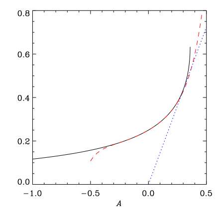
Figure 10: The numerically determined function of the amplitude $A$ that should equal $QA$ when the solvability condition for equation (171) is applied. The black solid line, which terminates at $A\approx 0.36$, shows the component of $\cos\tau$ in the Fourier series of $(1/4)\cos\tau\,H_{0}^{-1}$ determined from the numerical solution of equation (170). The red dashed line shows the series approximation given by the right-hand side of equation (174). The blue dotted line is of slope $1.45$ and passes through the origin.

The breakdown of the solution can be understood as a type of nonlinear resonance. It occurs while the nonlinear vertical oscillator exhibits a finite response, but the anharmonic and asymmetric character of that oscillator is essential to the behaviour.