A two-dimensional mixing length theory of convective transport

Abstract

The helioseismic observations of the internal rotation profile of the Sun raise questions about the two-dimensional (2D) nature of the transport of angular momentum in stars. Here we derive a convective prescription for axisymmetric (2D) stellar evolution models. We describe the small scale motions by a spectrum of unstable linear modes in a Boussinesq fluid. Our saturation prescription makes use of the angular dependence of the linear dispersion relation to estimate the anisotropy of convective velocities. We are then able to provide closed form expressions for the thermal and angular momentum fluxes with only one free parameter, the mixing length.

We illustrate our prescription for slow rotation, to first order in the rotation rate. In this limit, the thermodynamical variables are spherically symetric, while the angular momentum depends both on radius and latitude. We obtain a closed set of equations for stellar evolution, with a self-consistent description for the transport of angular momentum in convective regions. We derive the linear coefficients which link the angular momentum flux to the rotation rate ($\Lambda$- effect) and its gradient ($\alpha$-effect). We compare our results to former relevant numerical work.

1 Introduction

Computations in stellar evolution have generally been carried in one-dimensional (1D) frameworks. Since the seminal paper of Böhm-Vitense (1958), mixing length theory (MLT) has proved to be a very powerful tool to compute the transport of heat in stars, even though its underlying assumptions are very often regarded as crude in comparison to the complexity of the usually highly turbulent convective flows. Recently, it has also become clear from helioseismic observations that the rotational profile of the Sun is intrinsically two-dimensional (2D, see Schou & co authors, 1998, for example). Moreover, the inclusion of rotation in stars has been shown to be essential in many phases of stellar evolution (Meynet & Maeder, 1997; Yoon & Langer, 2004) but these simulations usually assume solid-body rotation within convective regions and a self-consistent treatment of rotation and convection is still lacking. We shall emphasise in this work that the characteristics of the angular momentum fluxes depend on the latitude even for spherically symmetric rotating stars. Indeed, the properties of the turbulent motions should naturally depend on the angle between the gravitational field and the angular velocity vector. It is thus clear that a proper treatment of the evolution of the rotation profile of stars requires a two-dimensional description. In this work we lay the basis of a self-consistent MLT formulation for 2D-axisymmetric rotating stars which could be adapted for future 2D stellar evolution computations. We illustrate our precriptions in the case of slow rotation, to first order in the rotation rate. In this limit we recover the classical 1D stellar evolution set of equations for spherically symetric stars with an additional 2D equation for angular momentum transport. We also provide a spherically averaged version for practical uses in current 1D stellar evolution codes including slow rotation, which allows for a self-consistent treatment of angular momentum transport in convective regions. We discuss our results in comparison to appropriate existing numerical simulations.

We start from the stellar fluid dynamical equations which we average on a smoothing length scale. Next, we consider the equations for perturbed quantities, for which we use a quasi-linear approximation: namely, we assume the perturbed fields are composed of a spectrum of unstable linear modes. Their amplitude is then determined by a saturation prescription which takes into accounts some of the non-linearities. We finally proceed to compute the heat and momentum fluxes which enter our averaged equations, thus closing our system. The only parameter in our model is the smoothing length scale, which we identify with the mixing length. This enables us to construct the stellar evolutionary equations without invoking additional parameters with accompanying assumptions.

Earlier Gough (1978) and Durney & Spruit (1979) developed very similar ideas but they adopted slightly different saturation prescriptions. They modelled the perturbed quantities with a single representative unstable mode with unspecified parameters to characterize its orientation whereas here we use the linear dispersion relation to infer the full spectrum of the perturbations. We therefore predict the anisotropy without extra parameters. An advantage of our approach is that it spells out the underlying assumptions which can then form the basis to improve the prescription. Ogilvie (2003) followed by Garaud et al. (2010) derived dynamical equations for the second order correlations supplemented by closure relations which introduce a set of additional non-dimensional parameters. Earlier, Canuto (1997) went even further in the hierarchy of correlations and provided a set of dynamical equations for quantities up to third order correlation terms with closure relations parametrized by even more free parameters. Kichatinov & Rudiger (1993) approximated the effects of turbulence by a viscous stress tensor and computed the effects of rotation on the momentum fluxes. Except for Canuto (1997), all these authors discussed only solid body rotation. We consider here the dynamics of convective motions in the presence of large-scale fields, such as non-uniform rotation and incorporate the presence of a shear in the calculation of turbulent fluxes.

In Section 2 we describe our framework in a Cartesian geometry and we present and discuss our MLT prescription, comparing it with the works of Gough (1978) and Durney & Spruit (1979). We apply it to slowly rotating spherical axisymmetric stars in Section 3. We discuss our results and conclusions in Section 4. In the Appendix, we give the full closed set of stellar evolution equations in the limit of slow rotation and we provide their spherically averaged equivalent for 1D stellar models.

2 General framework

We start with the equations of fluid dynamics subject to a local gravitational acceleration $\boldsymbol{g}$ with Cartesian components $g_{i}$. The mass conservation is given by

$$\partial_{t}\rho+\partial_{i}(\rho v_{i})=0,$$ (1)

where $\rho$ is the mass density, $v_{i}$ the components of the velocity and $\partial_{t}\equiv\partial/\partial t$ and $\partial_{i}\equiv\partial/\partial x_{i}$ are the partial derivatives with respect to time and each of the three spatial coordinates. We have used Einstein’s summation convention.

The momentum conservation leads to

$$\partial_{t}(\rho v_{i})+\partial_{j}(\rho v_{i}v_{j}+p\delta_{ij})=\rho g_{i},$$ (2)

where $p$ is the pressure and we have neglected viscosity.

The heat transport equation (see for example Landau & Lifshitz, 1987, equation 49.4) combined with continuity (equation 1) becomes

$$T\partial_{t}(\rho S)+T\partial_{j}(v_{j}\rho S)+\partial_{j}F_{j}=q,$$ (3)

where $S$ is the specific entropy, $q$ the net heat generation rate, $T$ the temperature and it is assumed there is no dependence of entropy on the chemical composition. The radiative flux is given by

$$F_{j}=-\rho c_{p}\chi\partial_{j}T$$ (4)

where $c_{p}$ is the heat capacity at constant pressure, $\chi$ is the thermal diffusivity (unit length $\times$ velocity). The spatial derivatives of both $c_{p}$ and $\chi$ are assumed to be negligible.

2.1 Average equations

We now define the sliding average of a quantity $y$ at position $\boldsymbol{x}$ by

$$\langle y\rangle=\frac{1}{\mathcal{V}}\int_{V(\boldsymbol{x})}y\,\mathrm{d}^{3}x$$ (5)

where $V(\boldsymbol{x})$ is a small cube of volume $\mathcal{V}$ centred on position $\boldsymbol{x}$. We want to find a new set of equations for the averaged quantities. These constitute our stellar model equations. We use as new variables the volume and mass weighted averages,

$$\bar{\rho}=\langle\rho\rangle,$$ (6)

$$\bar{v}_{i}=\frac{\langle\rho v_{i}\rangle}{\langle\rho\rangle}$$ (7)

and

$$\bar{e}=\langle\rho e\rangle/\langle\rho\rangle.$$ (8)

We then define the residuals with respect to these averages by

$$y^{\prime}=y-\bar{y}$$ (9)

for any quantity $y$.

We now make use of the Boussinesq approximations that velocities are small compared to the sound speed, wavelengths are small compared to the local scale height and $\rho^{\prime}\simeq 0$ except when coupled with the gravity $g_{i}$ (cf. Spiegel & Veronis, 1960). Although Gough (1969) has shown these approximations to be not suitable for stellar convective regions, and instead the anelastic approximation should be used, we feel they capture the essential physics while simplifying the derivation. In particular, these approximations allow us to work with nearly incompressible equations and to have $\langle y^{\prime}\rangle=0$ for most quantities of interest. With these approximations, the volume averaged continuity is unchanged,

$$\partial_{t}\bar{\rho}+\partial_{i}(\bar{\rho}\bar{v}_{i})=0.$$ (10)

The momentum equation becomes

$$\partial_{t}(\bar{\rho}\bar{v}_{i})+\partial_{j}(\bar{\rho}\bar{v}_{i}\bar{v}_{j}+\bar{p}\delta_{ij}+{\cal R}_{ij})=\bar{\rho}\bar{g}_{i},$$ (11)

where we discard $\langle\rho^{\prime}g^{\prime}\rangle$, because gravity is slowly varying and we use the convective momentum flux (more commonly referred to as the Reynolds stress tensor)

$${\cal R}_{ij}=\bar{\rho}\langle v^{\prime}_{i}v^{\prime}_{j}\rangle.$$ (12)

Finally the average entropy evolution equation is

$$\bar{T}\partial_{t}(\bar{\rho}\bar{S})+\bar{T}\partial_{j}(\bar{\rho}\bar{v_{j}}\bar{S}+\mathcal{F}_{j})+\partial_{j}F_{j}=\bar{q}$$ (13)

where, noting that $(\bar{T}+T^{\prime})^{-1}\approx\bar{T}^{-1}(1-T^{\prime}/T)$ we neglect the non-linear terms $\langle q^{\prime}T^{\prime}\rangle$ and $\langle T^{\prime}\partial_{j}F^{\prime}_{j}\rangle$, as is necessary to recover the classical formulation of MLT, and define the convective heat flux

$${\cal F}_{j}=\bar{\rho}\langle S^{\prime}v^{\prime}_{j}\rangle.$$ (14)

We drop the over bars in what follows to ease writing and reading but they should be assumed in the remainder of this section. In order to get expressions for the convective fluxes, we now turn to the estimation of the small scales (or $y^{\prime}$ ) quantities.

2.2 The sub-grid model

In order to make progress, we make assumptions about the linearity and scale of the perturbations. These are those usually made for a local mixing length theory. In the linear theory, we will then apply some kind of closure condition to determine the amplitudes of turbulent modes.

We appeal to the Boussinesq approximation and compute the difference between the general equations and their averages in order to obtain governing equations for the $y^{\prime}$ quantities. The continuity equation for the perturbed velocity becomes

$$\partial_{i}v^{\prime}_{i}=0.$$ (15)

The momentum equations yield

$$\partial_{t}(\rho v^{\prime}_{i})+\partial_{j}[\rho v_{i}\delta v_{j}+\rho v_{j}v^{\prime}_{i}+\rho v^{\prime}_{i}v^{\prime}_{j}+\delta p\delta_{ij}-{\cal R}_{ij}]=\rho^{\prime}g_{i},$$ (16)

where we have discarded $g^{\prime}$ because the gravitational field is produced by mass deep inside the star.

We now resort to a length scale separation hypothesis: averaged quantities are assumed to be nearly uniform in the local volume $V$ and perturbed quantities vary over scales that are much smaller than the diameter of $V$. Hence the gradient of ${\cal R}_{ij}$,

$$\partial_{j}{\cal R}_{ij}\ll\partial_{j}[\rho v_{i}v^{\prime}_{j}+\rho v_{j}v^{\prime}_{i}+\rho v^{\prime}_{i}v^{\prime}_{j}+p^{\prime}\delta_{ij}],$$ (17)

the gradients of the perturbed quantities. Mixing-length theories which make use of this approximation are generally called local mixing length theories. Most MLT used for practical purposes in stellar evolution are of this type.

We further neglect the non-linear terms and so set

$$\rho v^{\prime}_{i}v^{\prime}_{j}\approx 0$$ (18)

and retain only the linear approximation. In accord with the Boussinesq approximation we also neglect the temporal and spatial variation of the average mass density. Hence, the perturbed quantities are determined by solving the linear problem for the scales that fit well inside the local volume $V$ so that

$$\partial_{t}v^{\prime}_{i}+v^{\prime}_{j}\partial_{j}v_{i}+v_{j}\partial_{j}v^{\prime}_{i}+\frac{1}{\rho}\partial_{i}p^{\prime}=\frac{\rho^{\prime}}{\rho}g_{i}$$ (19)

where we have retained the shear term from the background velocity. This is necessary for the redistribution of angular momentum. With the Boussinesq approximation and neglecting the pressure perturbations with respect to thermal effects, we write the first law of thermodynamics as

$$S^{\prime}=c_{p}(\frac{T^{\prime}}{T}-\nabla_{\!\rm a}\frac{p^{\prime}}{p})\simeq c_{p}\frac{T^{\prime}}{T}$$ (20)

where $\nabla_{\!\rm a}=(\partial\log T/\partial\log p)_{S}$ is the usual adiabatic gradient. The entropy conservation equation is then linearised as

$$\partial_{t}\frac{T^{\prime}}{T}+{v}_{i}\partial_{i}\left(\frac{T^{\prime}}{T}\right)+\frac{1}{c_{p}}v^{\prime}_{i}\partial_{i}S=\chi\partial_{i}\partial_{i}\left(\frac{T^{\prime}}{T}\right),$$ (21)

where we have neglected $q^{\prime}$, the time-dependence of $c_{p}$ and the stratification in the thermal diffusion term. As is customary in mixing length theories, we have neglected the term

$$\frac{q}{\rho T}\left(\frac{q^{\prime}}{q}-\frac{\rho^{\prime}}{\rho}-\frac{T^{\prime}}{T}\right).$$ (22)

We simply note here that this term could become important when strong nuclear burning takes place within convective regions.

2.3 Saturation and amplitude of the linear modes

We restore some of the non-linear effects by adopting a strong assumption for the saturation of each mode. We denote by $\lambda_{\rm m}$ the smoothing length-scale, a typical scale of the smoothing volume $V$. At the largest scales within this volume, i.e. scales on the order of or just below the smoothing length scale $\lambda_{\rm m}$, we assume that the saturation of a given mode is due solely to its own shear. Parasitic instabilities, such as Kelvin-Helmholtz rolls, feed on the shear motions generated by the parent mode. We assume that eventually they are responsible for its saturation. We designate $\widetilde{\mn@boldsymbol{v^{\prime}}}_{\boldsymbol{k}}$ to be the complex amplitude of the Fourier mode of the velocity perturbation associated with a wave vector $\boldsymbol{k}$ and define the amplitude of the velocity perturbation

$$u_{\mn@boldsymbol{k}}=\sqrt{|\widetilde{v^{\prime}}_{1\boldsymbol{k}}|^{2}+|\widetilde{v^{\prime}}_{2\boldsymbol{k}}|^{2}+|\widetilde{v^{\prime}}_{3\boldsymbol{k}}|^{2}}.$$ (23)

We write schematically the time evolution of this amplitude by

$${\dot{u}_{\boldsymbol{k}}}\approx\sigma_{\boldsymbol{k}}u_{\boldsymbol{k}}-\sigma_{\mathrm{p}}(\boldsymbol{k},u_{\boldsymbol{k}})u_{\boldsymbol{k}}$$ (24)

where $\sigma_{\boldsymbol{k}}$ is the real part of the linear growth rate of the mode and $\sigma_{\mathrm{p}}(\boldsymbol{k},u_{\boldsymbol{k}})$ is the real part of the growth rate of the parasitic mode responsible for its saturation and we assume that $\sigma_{\mathrm{p}}$ depends only on $\boldsymbol{k}$ and on the amplitude $u_{\boldsymbol{k}}$ of the parent mode. For example, in the case of Kelvin-Helmholtz rolls, $\sigma_{\mathrm{p}}$ depends on the component of $\boldsymbol{k}$ orthogonal to $\boldsymbol{\widetilde{v^{\prime}}_{\mn@boldsymbol{k}}}$ but, because we have assumed that the motions are almost incompressible, $\sigma_{\mathrm{p}}$ is equal to $ku_{\mn@boldsymbol{k}}$ where $k=|\boldsymbol{k}|$ is the wave number. At saturation, equation (24) allows to write

$$\sigma_{\boldsymbol{k}}=\sigma_{\mathrm{p}}(\boldsymbol{k},u_{\boldsymbol{k}})$$ (25)

which determines the mode’s amplitude. For example, if Kelvin-Helmholtz is the dominant parasitic instability, the saturation is reached when the velocity is of the order of

$$u_{\boldsymbol{k}}=\sigma_{\boldsymbol{k}}/k.$$ (26)

Note that, provided $\sigma_{\boldsymbol{k}}$ depends on the direction of the wave vector $\boldsymbol{k}$, this prescription leads to an anisotropic amplitude of the velocity.

Similar ideas have been used to assess the saturation of other instabilities. The parasitic instabilities of the magnetorotational instability (MRI) were described by Goodman & Xu (1994) and Latter et al. (2009). Their role for the saturation of the MRI was examined independently by Lesaffre et al. (2009) and Pessah & Goodman (2009). The prescription we use here is very similar to that used by Pessah & Goodman (2009) and Pessah (2010). Guilet et al. (2010) have used a slight refinement of these prescriptions to predict the saturation amplitude of the standing accretion shock instability (SASI) in core-collapse supernovae. However, these ideas have so far been concerned with individual unstable modes. We propose here to extend this prescription to a whole spectrum of modes. At the largest scale we use the prescription (26). But the smallest scales are likely to feel the non-linear interactions of the scales immediately above and below, as in the Kolmogorov cascade (Kolmogorov, 1941). We therefore use a power-law scaling for each direction individually as a first approximation. We write $k_{\rm m}=\pi/\lambda_{\rm m}$ the minimum wave number in our smoothing volume. The resulting closure expression is then

$$u_{\boldsymbol{k}}=\left(\frac{k}{k_{\rm m}}\right)^{-n}\,\frac{1}{k_{\rm m}}\sigma_{\boldsymbol{k^{\prime}}},$$ (27)

where $\boldsymbol{k^{\prime}}=\frac{k_{\rm m}}{k}\boldsymbol{k}$ with $n=11/6$ for Kolmogorov scaling or $n=21/10$ for Bolgiano-Obukhov scaling (Bolgiano, 1959; Obukhov, 1959). These will likely bracket the actual spectrum index (see Rincon, 2006). The last factor accounts for the anisotropy of the driving instability and the first for the energy cascade. Our closure equation completely determines the amplitude of all Fourier coefficients of the velociy perturbations. Once the velocity amplitude is known, the linear system of equations for the perturbations is used to estimate the amplitude of all other perturbed variables relative to the velocity. The numerical study of Rincon (2006) has carefully examined the anisotropy and scaling of turbulent convection and we plan to validate our approach with such numerical studies. Note that the fluxes involve integrals of $u_{\boldsymbol{k}}^{2}\mathrm{d}^{3}k\propto k^{2-2n}dk$ for $k\geqslant k_{\rm m}$, so our results are only weakly sensitive to the exponent $n$ as long as it is strictly greater than $3/2$, otherwise these integrals diverge. This means that the fluxes are dominated by the largest scales just below the mixing length. In fact this conflicts with our assumption of scale separation but this is a common inconsistency of mixing length theories.

Others have avoided such divergent behaviour by considering only a limited number of modes. For example, in Gough’s (1978) statistical picture eddies of a given shape are randomly formed, grow and get disrupted whereas we envisage the sub-grid scale motions to be a collection of saturated unstable modes. Gough has an elaborate time-dependent model for the evolution of an eddy, whereas our work assumes a steady-state which saves us from specifying the initial conditions. For example, he has to assume seeds for the eddies to be isotropically distributed. Further, he has to prescribe a space filling factor for the shape of his representative eddy.

From equation (4.6) of Gough (1978), his definition of $\ell=\pi/k_{v}$ and if we identify his $\bar{w^{2}}$ with the square of the magnitude of the radial component of our velocity $|\widetilde{v^{\prime}}_{r\boldsymbol{k}}|^{2}$ and his $\sigma$ to our $\sigma_{\boldsymbol{k}}$, we arrive at

$$|\widetilde{v^{\prime}}_{r\boldsymbol{k}}|^{2}=\Lambda\pi^{2}\sigma_{\boldsymbol{k}}^{2}(k_{h}^{2}/k^{4}),$$ (28)

where $k_{h}$ is the magnitude of the horizontal part of the representative wave vector and $\Lambda$ is a calibrateable dimensionless constant which incorporates the anisotropy parameter as well as the filling factor.

Durney & Spruit (1979) have also proposed a similar saturation prescription to ours. They set

$$\langle{v^{\prime}}_{r}^{2}\rangle=\langle\sigma_{\boldsymbol{k}}^{2}\rangle\pi^{2}/k_{r}^{2}$$ (29)

for a linear combination of a few modes with similar wave vectors. Both these prescriptions slightly differ mathematically from ours. However, the fundamental difference lies in the existence of a parameter which prescribes the anisotropy of the velocity field in both the works of Gough (1978) and Durney & Spruit (1979), whereas our prescription links this anisotropy to physics of the underlying instability which generates the perturbations.

2.4 Computation of the fluxes

We have hitherto discussed how to determine the modulus of all the Fourier coefficients of the perturbations. We now summarize how to compute the convective fluxes, which depend on the volume average of a product of two perturbed quantities:

$$\langle y^{\prime}z^{\prime}\rangle=\frac{1}{\mathcal{V}}\int_{V}y^{\prime}z^{\prime}\,{\rm d}^{3}x\mbox{.}$$ (30)

We assume the volume $V$ is a cube of side $\lambda_{\rm m}$, hence $\mathcal{V}=\lambda_{\rm m}^{3}$. Any field on this cube can be represented by its Fourier modes with wave number coordinates as multiples of $k_{\rm m}=\pi/\lambda_{\rm m}$, for instance:

$$y^{\prime}(\mn@boldsymbol{x})=\sum_{\mn@boldsymbol{k}/k_{\rm m}\in\mathbb{Z}^{3}}\widetilde{y^{\prime}}_{\mn@boldsymbol{k}}e^{i\mn@boldsymbol{k.x}}\mbox{.}$$ (31)

where $\widetilde{y^{\prime}}$ denotes the Fourier transform of $y^{\prime}$. We use Parseval’s theorem to write

$$\int_{V}y^{\prime}z^{\prime*}\,{\rm d}^{3}x=\lambda_{\rm m}^{3}\sum_{\mn@boldsymbol{k}/k_{\rm m}\in\mathbb{Z}^{3}}\widetilde{y^{\prime}}_{\mn@boldsymbol{k}}\widetilde{z^{\prime}}^{*}_{\mn@boldsymbol{k}}$$ (32)

and

$$\int_{V}y^{\prime*}z^{\prime}\,{\rm d}^{3}x=\lambda_{\rm m}^{3}\sum_{\mn@boldsymbol{k}/k_{\rm m}\in\mathbb{Z}^{3}}\widetilde{y^{\prime}}^{*}_{\mn@boldsymbol{k}}\widetilde{z^{\prime}}_{\mn@boldsymbol{k}}\mbox{.}$$ (33)

We take the average of the two previous equations and use the fact that $y^{\prime}$ and $z^{\prime}$ are real fields to get

$$\int_{V}y^{\prime}z^{\prime}\,{\rm d}^{3}x=\lambda_{\rm m}^{3}\sum_{\mn@boldsymbol{k}/k_{\rm m}\in\mathbb{Z}^{3}}|\widetilde{y^{\prime}}_{\mn@boldsymbol{k}}||\widetilde{z^{\prime}}_{\mn@boldsymbol{k}}|\cos(\psi(\mn@boldsymbol{k}))$$ (34)

where $\psi(\mn@boldsymbol{k})$ is the phase difference between $\widetilde{y^{\prime}_{\mn@boldsymbol{k}}}$ and $\widetilde{z^{\prime}_{\mn@boldsymbol{k}}}$. We estimate this phase difference from the linear analysis of the corresponding mode.

Finally, we approximate the sum on all wave vectors by a continuous integral over the non-dimensional wave-vector $\widetilde{\mn@boldsymbol{k}}=\mn@boldsymbol{k}/k_{\rm m}$:

$$\langle y^{\prime}z^{\prime}\rangle=\int_{|\widetilde{\mn@boldsymbol{k}}|>1}|\widetilde{y^{\prime}}_{\widetilde{\mn@boldsymbol{k}}}||\widetilde{z^{\prime}}_{\widetilde{\mn@boldsymbol{k}}}|\cos(\psi(\widetilde{\mn@boldsymbol{k}}))\,{\rm d}^{3}\widetilde{k}\mbox{.}$$ (35)

3 Slowly rotating axisymmetric stars

The local rotation rate $\Omega$ of a star can be compared to two rates of interest to construct dimensionless numbers. On the one hand, the inverse of the free-fall time scale yields $\epsilon_{0}=\Omega\sqrt{r/g}$, while the buoyancy frequency provides another number $\epsilon=\Omega/N$ where $N$ is the magnitude of the Brunt-Väisälä frequency. The latter can also be written $\epsilon=\Omega\sqrt{H_{S}/g}$ where $H_{S}$ is on the order of the entropy scale height. Although most stars have $\epsilon_{0}\ll 1$, the entropy mixing in convective regions can make $H_{S}$ very large and $\epsilon$ is not necessarily close to zero. For example, our Sun has $\epsilon_{0}=7.4\times 10^{-4}$ at the surface, but $\epsilon$ can be of order unity at the bottom of the convective region. In the following, we derive the stellar evolution equations to first order in the parameter $\epsilon$ and assume $\epsilon_{0}<\epsilon$. We will further assume that the tides are weak and that an axisymmetric model about the rotation axis can suffice.

3.1 Background state

In such an axisymmetric star, it is natural to use a spherical coordinate system, with $r$, $\theta$ and $\phi$ as the radius, co-latitude and azimuth respectively, for the definition of the background. The hydrostatic pressure balance with centrifugal acceleration necessarily implies that the deviation from spherical symetry in the thermodynamic quantities $p$ and $\rho$ is on the order of $\epsilon_{0}^{2}$. In the first order we can therefore safely assume that the thermal background depends on the radius $r$ only and that the gravitational acceleration is radial. Similarly, since meridional circulation is the result of second order terms ($\Omega^{2}$), we neglect it. Then the averaged velocity profile consists only of cylindrical rotation so that

$$\bar{v}_{\phi}=r\Omega(r,\theta)\sin\theta$$

and

$$\bar{v}_{r}=\bar{v}_{\theta}=0.$$

According to our assumptions the background must be smooth over the scale of the volume $V$. This requires that the first derivative of $\Omega$ with respect to the cylindrical radius is zero on the axis of symmetry.

3.2 Linear System of equations for the modes

We develop the perturbation at a position $\boldsymbol{x_{0}}$ in terms of local Fourier modes in a local Cartesian frame rotating about the axis of symmetry with angular velocity $\Omega_{0}=\Omega(\boldsymbol{x_{0}})$. The three axes of the frame $\hat{\mn@boldsymbol{x}}$, $\hat{\mn@boldsymbol{y}}$ and $\hat{\mn@boldsymbol{z}}$ are made to coincide with the local spherical coordinate unit vectors, $\hat{\mn@boldsymbol{r}}$, $\hat{\mn@boldsymbol{\theta}}$ and $\hat{\mn@boldsymbol{\phi}}$ at $\boldsymbol{x_{0}}$. We consider only one single mode in this subsection. Thus

$$y^{\prime}_{\boldsymbol{k}}\equiv\Re[\widetilde{y^{\prime}}_{\boldsymbol{k}}\,\exp(st+ik_{x}x+ik_{y}y+ik_{z}z)],$$ (36)

where $\widetilde{y^{\prime}}_{\boldsymbol{k}}$ is the complex amplitude of the mode under consideration, $i=\sqrt{-1}$ , $x$, $y$ and $z$ are the coordinates in this local Cartesian frame and $k_{x}$, $k_{y}$ and $k_{z}$ are the three components of the wave vector in this frame. The three coordinates have the physical dimension of the radius $r.$ In particular, $\mathrm{d}x=\mathrm{d}r$, $\mathrm{d}y=r\mathrm{{}_{0}d}\theta$ and $\mathrm{d}z=r_{0}\sin\theta_{0}\mathrm{d}\phi$. In principle, shear deforms non-axisymmetric perturbations on a time scale of the order of the local shear time, which we therefore assume to be long compared with the growth time $\Re(s)^{-1}$ in order to apply our linear analysis. Although this is true for the Sun now, it may not necessarily hold for all stars. It certainly is not true for Keplerian discs, where the shear rate is comparable to the rotation rate and to the inverse of the vertical convective turnover time-scale. We shall drop the $\boldsymbol{k}$ subscripts from the complex amplitudes in this section and the next in order to ease the readability.

The linearised continuity equation (15) leads to the incompressibility condition

$$k_{x}\widetilde{v^{\prime}}_{r}+k_{y}\widetilde{v^{\prime}}_{\theta}+k_{z}\widetilde{v^{\prime}}_{\phi}=0.$$ (37)

The momentum equation (19) now includes an additional Coriolis term $2\boldsymbol{\Omega}_{0}\times\boldsymbol{v^{\prime}}$ because the background velocity in the rotating frame is $\bar{v}_{\phi}=r\sin\theta[\Omega(r,\theta)-\Omega_{0}]$. We assume that the apparent gravitational field (including centrifugal acceleration) is vertical and write $g=g_{r}$, in accordance with our first order expansion in the rotation rate. The linearised Euler equations become

$$s\widetilde{v^{\prime}}_{r}-2\Omega_{0}\sin\theta_{0}\,\widetilde{v^{\prime}}_{\phi}=-\frac{ik_{x}}{\rho}p^{\prime}-g\frac{\rho^{\prime}}{\rho},$$ (38)

$$s\widetilde{v^{\prime}}_{\phi}-2\Omega_{0}\cos\theta_{0}\,\widetilde{v^{\prime}}_{\phi}=-\frac{ik_{y}}{\rho}p^{\prime}$$ (39)

and

$$s\widetilde{v^{\prime}}_{\phi}+2\Omega_{0}M_{r}\widetilde{v^{\prime}}_{r}+2\Omega_{0}M_{\theta}\widetilde{v^{\prime}}_{\theta}=-\frac{ik_{z}}{\rho}p^{\prime},$$ (40)

where

$$M_{r}=\frac{1}{2\Omega r\sin\theta_{0}}\partial_{r}j$$ (41)

and

$$M_{\theta}=\frac{1}{2\Omega r^{2}\sin\theta_{0}}\partial_{\theta_{0}}j$$ (42)

and the specific angular momentum $j$ is

$$j=r^{2}\Omega\sin^{2}\theta_{0}.$$ (43)

Here, $M_{r}$ and $M_{\theta}$ are two dimensionless quantities proportional to the spherical coordinates of the gradient of specific angular momentum at our reference point so that

$$\boldsymbol{M}=\frac{1}{2\Omega r\sin\theta_{0}}\boldsymbol{\nabla}j.$$ (44)

For uniform rotation, this vector is simply $\boldsymbol{M}=\boldsymbol{\hat{R}}$ where $\boldsymbol{\hat{R}}$ is the cylindrical radius unit vector.

The Boussinesq approximation means that pressure perturbations are negligible when compared to density and thermal perturbations. So the equation of state becomes

$$\frac{\rho^{\prime}}{\rho}+\Delta\frac{T^{\prime}}{T}=0,$$ (45)

where

$$\Delta=-\left(\frac{\partial\ln\rho}{\partial\ln T}\right)_{p}$$ (46)

is the compressibility at constant pressure.

Finally, the entropy equation (21) becomes

$$(s+\chi k^{2})\frac{T^{\prime}}{T}=-\frac{1}{g\Delta}N^{2}\widetilde{v^{\prime}}_{r},$$ (47)

where

$$k^{2}=k_{x}^{2}+k_{y}^{2}+k_{z}^{2}$$ (48)

is the square of the modulus of the wave vector and the thermal Brunt-Väisälä frequency $N^{2}$ is

$$N^{2}=\frac{g\Delta}{c_{p}}\partial_{r}S$$ (49)

where we neglect the latitudinal thermal gradients, in accordance with our first order expansion in the rotation frequency. In the following, we drop the $0$ subscripts of $\theta$ and $\boldsymbol{M}$ for the sake of tidiness.

3.3 Dispersion relation and growth rate

The set of linear equations (37) to (47) forms an eigenvalue problem for $s$. Its dispersion relation is a cubic in $s$ which we express as:

$$s^{3}+ [1-(\hat{\mn@boldsymbol{k}}.\hat{\mn@boldsymbol{r}})^{2}]N^{2}s$$

$$+ 2\Omega(\hat{\mn@boldsymbol{k}}.\hat{\mn@boldsymbol{\phi}})(\hat{\mn@boldsymbol{R}}-\hat{\mn@boldsymbol{M}}).[s^{2}\hat{\mn@boldsymbol{k}}+(\hat{\mn@boldsymbol{k}}.\hat{\mn@boldsymbol{\theta}})N^{2}\hat{\mn@boldsymbol{\theta}}]+4\Omega^{2}(\hat{\mn@boldsymbol{k}}.\hat{\mn@boldsymbol{\Omega}})\hat{\mn@boldsymbol{k}}.(\hat{\mn@boldsymbol{M}}\times\hat{\mn@boldsymbol{\phi}})\,s$$

$$+ \chi k^{2}[s^{2}+2\Omega\hat{\mn@boldsymbol{k}}.(\hat{\mn@boldsymbol{R}}-\hat{\mn@boldsymbol{M}})s+2\Omega^{2}(\hat{\mn@boldsymbol{k}}.\hat{\mn@boldsymbol{\Omega}})\hat{\mn@boldsymbol{k}}.(\hat{\mn@boldsymbol{M}}\times\hat{\mn@boldsymbol{\phi}})]=0$$ (50)

where $\hat{\mn@boldsymbol{k}}$ and $\hat{\mn@boldsymbol{\Omega}}$ are the unit vectors along $\mn@boldsymbol{k}$ and $\mn@boldsymbol{\Omega}$. Without thermal diffusion, this dispersion relation depends only on the direction of the wave vector $\hat{\mn@boldsymbol{k}}$ and not on its magnitude. For uniform rotation ($\hat{\mn@boldsymbol{M}}=\hat{\mn@boldsymbol{R}}$) and $\chi=0$, we recover the results from both Cowling (1951) and Durney & Spruit (1979). For axisymmetric modes ($\hat{\mn@boldsymbol{k}}.\hat{\mn@boldsymbol{\phi}}=0$), we recover the dispersion relation of Goldreich & Schubert (1967) without viscosity.

We now set $\chi=0$ and turn to evaluate the largest real part of the roots of the dispersion relation. We will seek the first order expansion of the growth rate in the form $s=Ns_{0}+\Omega s_{1}=N(s_{0}+\epsilon s_{1})$. For the largest real root at zeroth order, we get

$$s_{0}=\sqrt{1-(\hat{\mn@boldsymbol{k}}.\hat{\mn@boldsymbol{r}})^{2}}$$ (51)

provided $N^{2}<0$, which is the condition for instability. This expression shows that the fastest growing modes have zero radial wave number so that vertical convective plumes are preferred. Our saturation prescription based on the directional dependence of the growth rate will be sensitive to this.

The first order of the largest real root is

$$s_{1}=(\hat{\mn@boldsymbol{k}}.\hat{\mn@boldsymbol{\phi}})(\hat{\mn@boldsymbol{R}}-\hat{\mn@boldsymbol{M}}).[\hat{\mn@boldsymbol{k}}+\frac{\hat{\mn@boldsymbol{k}}.\hat{\mn@boldsymbol{\theta}}}{1-(\hat{\mn@boldsymbol{k}}.\hat{\mn@boldsymbol{r}})^{2}}\hat{\mn@boldsymbol{\theta}}].$$ (52)

Close to marginal stability, the marginal root $s_{\rm m}=0$ without rotation can have the largest real part for slow rotation. However, $s_{\rm m}$ is first order in $\epsilon$ and the associated fluxes are of order $\epsilon^{2}$ and we safely neglect it.

Finally, since $s_{0}$ and $s_{1}$ are always real, we simply take

$$\sigma_{\mn@boldsymbol{k}}=N(s_{0}+\epsilon s_{1})$$ (53)

when $N^{2}<0$ and $\sigma_{\mn@boldsymbol{k}}=0$ otherwise.

3.4 Convective fluxes

Both the first and second order of the growth rate are real numbers, consequently the linear system of equations (37) to (47) introduces no phase shift between the perturbed fields involved. In our notations, the phase shift which enters the expression (35) for the flux is $\psi(\mn@boldsymbol{k})=0$ or $\pi$ for all pairs of variables of interest.

3.4.1 Kinetic energy

We start by deriving a useful relation between variables $\widetilde{v^{\prime}}_{r}$ and $\widetilde{v^{\prime}}_{\theta}$. We use equation (37) to express the variable $\widetilde{v^{\prime}}_{\phi}$ in terms of the other two components of the velocity. Then, we combine equations (39) and (40) to eliminate the variable $p^{\prime}$ and so find the relationship between $\widetilde{v^{\prime}}_{r}$ and $\widetilde{v^{\prime}}_{\theta}$ to be

$$-[\alpha\beta s- \beta\gamma 2\Omega M_{r}+\alpha\gamma 2\Omega\cos\theta]\widetilde{v^{\prime}}_{r}$$

$$=[(1-\alpha^{2})s- \beta\gamma 2\Omega M_{\theta}+\beta\gamma 2\Omega\cos\theta]\widetilde{v^{\prime}}_{\theta}.$$ (54)

where we defined the more compact variables

$$\alpha= \hat{\mn@boldsymbol{k}}.\hat{\mn@boldsymbol{r}}=k_{x}/k,$$ (55)

$$\beta= \hat{\mn@boldsymbol{k}}.\hat{\mn@boldsymbol{\theta}}=k_{y}/k\mbox{ and}$$ (56)

$$\gamma= \hat{\mn@boldsymbol{k}}.\hat{\mn@boldsymbol{\phi}}=k_{z}/k.$$ (57)

Here $\alpha^{2}+\beta^{2}+\gamma^{2}=1$.

We now develop to first order in $\epsilon$ the ratio of $\widetilde{v^{\prime}}_{\theta}$ over $\widetilde{v^{\prime}}_{r}$ from relation (54) to formally obtain

$$\widetilde{v^{\prime}}_{\theta}/\widetilde{v^{\prime}}_{r}=-\frac{\alpha\beta}{\beta^{2}+\gamma^{2}}+\gamma\epsilon f(\alpha^{2},\beta^{2}),$$ (58)

where $f$ is a complicated function of $\alpha^{2}$ and $\beta^{2}$ of order 1. The terms involving $s_{1}$ cancel. We now use equation (37) to get

$$\widetilde{v^{\prime}}_{\phi}/\widetilde{v^{\prime}}_{r}=-\frac{\alpha\gamma}{\beta^{2}+\gamma^{2}}+\gamma\epsilon f(\alpha^{2},\beta^{2})$$ (59)

and we apply our saturation prescription (27) to arrive at

$$\sigma_{\boldsymbol{k^{\prime}}}^{2}k_{\rm m}^{-2}\tilde{k}^{-2n}=|\widetilde{v^{\prime}}_{r}|^{2}+|\widetilde{v^{\prime}}_{\theta}|^{2}+|\widetilde{v^{\prime}}_{\phi}|^{2}=\widetilde{v^{\prime}}_{r}^{2}\,(1-4\epsilon\alpha\beta\gamma f)/(\beta^{2}+\gamma^{2}).$$ (60)

In the expression (35) we separate the integral over the magnitude of the wave vector from the integral over all possible directions of the wave vector. We determine that

$$\langle v_{r}^{{}^{\prime}2}\rangle=\int_{1}^{+\infty}\frac{N^{2}}{k_{\rm m}^{2}}\tilde{k}^{-2n}\,4\pi\tilde{k}^{2}\mathrm{d}\tilde{k}\,\int_{\alpha^{2}+\beta^{2}+\gamma^{2}=1}s_{0}^{2}(\beta^{2}+\gamma^{2})\,\frac{\mathrm{d}\alpha\mathrm{d}\beta\mathrm{d}\gamma}{4\pi}$$ (61)

to the lowest (zeroth) order in $\epsilon$ and we use $\tilde{k}=k/k_{\rm m}$. The first order in $\epsilon$ is odd in $\gamma$ and its integration over the unit sphere yields a zero contribution. We perform the integral on the non-dimensional modulus of the wave vector $\tilde{k}$ and write

$$\langle v_{r}^{{}^{\prime}2}\rangle=\frac{4N^{2}\lambda_{\rm m}^{2}}{\pi(2n-3)}\,F_{rr}$$ (62)

with

$$F_{rr}=\langle s_{0}^{4}\rangle_{\rm S}\simeq 0.533$$ (63)

where $\langle\rangle_{\rm S}$ denotes averaging over the unit sphere and we used $s_{0}^{2}=1-\alpha^{2}=\beta^{2}+\gamma^{2}$. With Kolomogorov scaling ($n=11/6$),

$$\langle v_{r}^{{}^{\prime}2}\rangle=\frac{6}{\pi}\lambda_{\rm m}^{2}N^{2}F_{rr}.$$ (64)

Note that with Bolgiano-Obukhov scaling ($n=21/10$), the prefactor $6/\pi$ decreases to $10/3\pi$ which is about twice smaller. We retain Kolomogorov scaling in the following. The other diagonal components of the Reynolds-stress tensor are

$$\langle v_{\theta}^{{}^{\prime}2}\rangle=\frac{6}{\pi}\lambda_{\rm m}^{2}N^{2}F_{\theta\theta},$$ (65)

with

$$F_{\theta\theta}=\langle\alpha^{2}\beta^{2}\rangle_{\rm S}$$ (66)

and

$$\langle v_{\phi}^{{}^{\prime}2}\rangle=\frac{6}{\pi}\lambda_{\rm m}^{2}N^{2}F_{\phi\phi},$$ (67)

with

$$F_{\phi\phi}=\langle\alpha^{2}\gamma^{2}\rangle_{\rm S}=F_{\theta\theta}\simeq 0.067.$$ (68)

Our model predicts a strong anisotropic distribution of velocities with motions mostly in the radial direction. In accordance with the symetry of the problem, our model predicts equipartition between the azimuthal and latitudinal directions.

Käpylä et al. (2004) compute these quantities in a number of simulations of convection including rotation. Our small parameter $\epsilon=\Omega/N$ translates in their notations as $\epsilon=\frac{1}{2}(\frac{PrTa}{Ra})^{\frac{1}{2}}$. Their simulation with $Co=1$ corresponds to our $\epsilon=0.09$. On the other hand we need the thermal diffusion timescale to be small before the rotation timescale because we neglected thermal diffusion (and viscosity), and we require $\chi/H_{p}^{2}/\Omega$ to be small where $H_{p}$ is the pressure scale height. The value of this parameter is $0.17$ for their simulation with $Co=1$ and bigger for lower rotation rates, so we consider only their results at $Co=1$. Using $\lambda_{\rm m}=\frac{1}{2}H_{p}$ in equations (64), (65) and (67) we find $\langle\mn@boldsymbol{{v^{\prime}}^{2}}\rangle^{\frac{1}{2}}=0.120$ which is only slightly bigger than the value $0.090$ which they find (viscous damping or a smaller $\lambda_{\rm m}$ could bring these values closer to one another). We also predict the ratio of horizontal to vertical motions $\langle v^{\prime}_{\theta}v^{\prime}_{\theta}+v^{\prime}_{\phi}v^{\prime}_{\phi}\rangle/\langle v^{\prime}_{r}v^{\prime}_{r}\rangle=0.125$ instead of their value of 0.186. Our saturation prescription probably overestimates the anisotropy because it neglects the tendency to isotropy at small scales down the turbulent cascade (cf. Rincon, 2006). Nevertheless, our model correctly accounts for the fact that the anisotropy does not depend on the latitude.

3.4.2 Thermal fluxes

From equation (47), we write

$$\langle\frac{T^{\prime}}{T}v^{\prime}_{i}\rangle=\frac{6}{\pi}\frac{\lambda_{\rm m}^{2}N^{3}}{g}F_{Ti},$$ (69)

with

$$F_{Tr}=\langle s_{0}^{3}\rangle_{\rm S}\simeq 0.589$$ (70)

and

$$F_{T\theta}=-\langle s_{0}\alpha\beta\rangle_{\rm S}=0$$ (71)

to the lowest order in $\epsilon$. The latitudinal thermal flux is zero to first order, consistent with the direction of the thermal gradients being vertical.

The average equation for the evolution of thermal energy is

$$T\partial_{t}S+\frac{T}{r^{2}}\partial_{r}(r^{2}{\cal F}_{r})-\boldsymbol{\nabla.}(\rho c_{p}\chi\boldsymbol{\nabla}T)=q,$$ (72)

with the thermal convective flux given by

$${\cal F}_{r}=\frac{1}{2}\rho c_{p}\int_{0}^{\pi}d\theta\,\sin\theta\langle v^{\prime}_{r}\frac{T^{\prime}}{T}\rangle.$$ (73)

Using equation (69) we write

$${\cal F}_{r}=\rho c_{p}\,\frac{6}{\pi}\,F_{Tr}\,\frac{\lambda_{\rm m}^{2}N^{3}}{g},$$ (74)

which we further develop into the more familiar thermal diffusive flux

$${\cal F}_{r}=-D_{T}\,\rho c_{p}\,\Delta\partial_{r}S,$$ (75)

with the effective diffusion coefficient

$$D_{T}=\frac{6}{\pi}\,F_{Tr}\,N\lambda_{\rm m}^{2}\simeq 0.68N\lambda_{\rm m}^{2}$$ (76)

MLTs traditionally make use of a diffusion coefficient of the form

$$D_{\rm MLT}=\frac{1}{3}N\ell_{\rm mix}^{2}$$ (77)

where $\ell_{mix}$ is the mixing length. Comparing this expressions to the usual 1D MLT, we can readily identify our smoothing length $\lambda_{\rm m}$ with the mixing length to a numerical factor of order one.

In the simulations of Käpylä et al. (2004) with $Co=1$, they compute the eddy heat conductivity, $\chi_{rr}=\langle v^{\prime}_{r}T^{\prime}/T\rangle g/N^{2}$ in our notations. They compute the ratio $\chi_{rr}/\nu_{t}$ where $\nu_{t}=\langle{v^{\prime}}^{2}\rangle^{\frac{1}{2}}d/3$ and $d$ is the size of the convective zone (see their figure 19) and find it is between 0.5 and 0.6 depending on the latitude. With $\lambda_{\rm m}=\frac{1}{2}H_{p}$, we predict a slightly bigger value of 0.67 for this number, which is overestimated by about the same factor than for the r.m.s. velocity (a lower value for $\lambda_{\rm m}$ would fix both numbers at the same time).

3.4.3 Momentum fluxes

The expressions for momentum fluxes are a bit more complicated. It has become common practice (see Rüdiger, 1989) to separate the momentum fluxes into a term linear in the rotation frequency (the $\Lambda$-effect) and a term which depends on the gradients of the rotation frequency ($\alpha$-effect), rather than the gradients of specific angular momentum which we have used here. Therefore we offset the quantities $M_{r}$ and $M_{\theta}$ by their respective values for solid body rotation to compare more directly with previous work. Each momentum flux develops into a linear combination of terms, characterized by four constant coefficients. For instance, we develop the radial momentum flux as

$$\frac{\langle v^{\prime}_{r}v^{\prime}_{\phi}\rangle}{\frac{6}{\pi}\lambda_{\rm m}^{2}N\Omega}=F_{r\phi,Mr}(M_{r}-\sin\theta)+F_{r\phi,M\theta}(M_{\theta}-\cos\theta)+F_{r\phi,\cos\theta}\cos\theta+F_{r\phi,\sin\theta}\sin\theta.$$ (78)

Since $F_{r\phi,M\theta}=F_{r\phi,\cos\theta}=0$, this reduces to

$${\langle v^{\prime}_{r}v^{\prime}_{\phi}\rangle}={\frac{6}{\pi}\lambda_{\rm m}^{2}N\Omega}\,(\frac{1}{2}F_{r\phi,Mr}\frac{\partial\ln\Omega}{\partial\ln r}+F_{r\phi,\sin\theta})\,\sin\theta$$ (79)

with

$$F_{r\phi,Mr}=\langle-2s_{0}^{3}(\alpha^{2}+\beta^{2})\rangle_{\rm S}\simeq-0.687,$$ (80)

and

$$F_{r\phi,\sin\theta}=\langle-2s_{0}\beta^{2}\rangle_{\rm S}=\langle-s_{0}^{3}\rangle_{\rm S}=-F_{Tr}\simeq-0.589.$$ (81)

The two terms in expression (79) represent respectively the $\alpha$-effect and the $\Lambda$-effect (see Rüdiger, 1989). The radial $\alpha$-effect is linked to differential rotation and is diffusive in character. This was also found by Houdek & Gough (2001) at the equator ($\theta=\pi/2$), but some quantities in their expression are defined only implicitly which makes a direct comparison difficult. In the case of solid body rotation, we predict a $\Lambda$-effect in the form

$$\Lambda_{r\phi}=\frac{6}{\pi}\,F_{r\phi,\sin\theta}\,\lambda_{\rm m}^{2}N\Omega\sin\theta\simeq-1.12\lambda_{\rm m}^{2}N\Omega\sin\theta.$$ (82)

This compares very well with the work of both Kichatinov & Rudiger (1993) and Garaud et al. (2010) in the slow rotation limit (see in particular equations (75) and (76) of Garaud et al., 2010). However, we note the $\Lambda$-effect of Kichatinov & Rudiger (1993) is essentially due to density gradients which we have neglected here, and they find a $\Lambda$-effect with the opposite sign compared to us. Note that Garaud et al. (2010) present their results as a function of anisotropy but, as they point out, the anisotropy is not arbitrary in their framework as in ours. In effect, the numerical coefficient in front of their $\Lambda$-term depends on the values of their closure parameters $C_{1}$, $C_{2}$, $C_{6}$ and $C_{7}$ and their expression does not differ from that of Kichatinov & Rudiger (1993), except possibly for the numerical value of the pre-factor and the sign which could be either positive or negative. Although the notion of a $\Lambda$-term was not used at that time, both Gough (1978) and Durney & Spruit (1979) have such a term in their formulation and correctly estimate its form in the slow rotation limit.

Simulations of Chan (2001), Rieutord et al. (1994) and Käpylä et al. (2004) all find a negative $\Lambda$-effect for slow rotation, in agreement with our results. However, we over-estimate by a large amount (up to a factor 4 near the equator) the value of the transport coefficient compared to the simulations of Käpylä et al. (2004), as seen in figure 1. The numbers extracted from the simulations are corrected from large scale shear flows which appear in their simulations. We use the numbers from their table 3, which shows the corrections themselves are of the same order as the measured radial momentum fluxes.

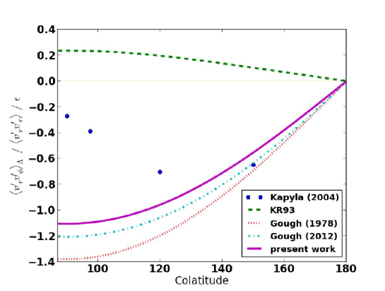
Figure 1: Normalised radial angular momentum flux due to the $\Lambda$-effect, $\langle v^{\prime}_{r}v^{\prime}_{\phi}\rangle_{\Lambda}/\langle v^{\prime}_{r}v^{\prime}_{r}\rangle/\epsilon$, according to simulations in Käpylä et al. (2004) (blue dots), to the predictions of Kichatinov & Rudiger (1993) (green), to both predictions by Gough (1978) (red, first order in $\epsilon$), Gough (2012) (cyan) and to our predictions (magenta). The numbers from the numerical simulations are corrected from the shear (see table 3 in Käpylä et al., 2004). To plot the results by Kichatinov & Rudiger (1993), we use the effective viscosity $\nu_{t}$ defined as $\nu_{t}=\langle{v^{\prime}}^{2}\rangle^{\frac{1}{2}}d/3$ where $d$ is the size of the convective region in their numerical setup and we took $\langle v^{\prime}_{r}v^{\prime}_{r}\rangle$ as measured in the simulations by Käpylä et al. (2004). To plot the results by Gough, we used the parameter $\Phi=1.9$ as measured from the simulations.

In a similar way we write the latitudinal momentum flux as

$${\langle v^{\prime}_{\theta}v^{\prime}_{\phi}\rangle}={\frac{6}{\pi}\lambda_{\rm m}^{2}N\Omega}\,\frac{1}{2}F_{\theta\phi,M\theta}\frac{\partial\ln\Omega}{\partial\theta}\sin\theta$$ (83)

with

$$F_{\theta\phi,M\theta}=\langle\frac{2}{s_{0}^{3}}\alpha^{2}\beta^{2}(\gamma^{4}-\alpha^{2}\beta^{2}-\beta^{4})\rangle_{\rm S}\simeq-0.123.$$ (84)

The latitudinal $\alpha$-effect is also diffusive but with a diffusion coefficient about six times smaller than the radial one. The latitudinal $\Lambda$-effect for solid body rotation and our vertical entropy gradient is absent to first order in $\Omega$. This is in agreement with all of Gough (1978), Durney & Spruit (1979), Kichatinov & Rudiger (1993) and Garaud et al. (2010), though in the case of Durney & Spruit (1979) the latitudinal-azimuthal balance of kinetic energy is needed to cancel this term. This is also consistent with the results of Käpylä et al. (2004) who find this term is much smaller than its radial counterpart in the limit of slow rotation.

The average equation for the transport of angular momentum can be found in Durney (1985) (equation (3)). To first order the meridional circulation is absent and with our notations the angular momentum transport equation may be written as

$$\rho\partial_{t}r^{2}\sin^{2}\theta\,\Omega+\frac{\sin\theta}{r^{2}}\partial_{r}(r^{3}\,{\cal R}_{r\phi})+\frac{1}{\sin\theta}\partial_{\theta}(\sin^{2}\theta\,{\cal R}_{\phi\theta})=0$$ (85)

We now consider the special case of spherical symmetry which is more useful for 1D stellar evolution codes. For this purpose we take $\Omega$ to be a function of $r$ only, so $M_{\theta}=\cos\theta$ and the latitudinal transport of momentum vanishes. It is however customary to integrate equation (85) over the angles $\frac{1}{r}\int_{0}^{\pi}d\theta\,\sin\theta\,\times...$ in order to eliminate the $\partial_{\theta}$ term so that

$$\rho\frac{4}{3}r^{2}\partial_{t}\Omega+\frac{1}{r^{2}}\partial_{r}(r^{3}\bar{\cal R}_{r\phi})=0,$$ (86)

with

$$\bar{\cal R}_{r\phi}=\int_{0}^{\pi}d\theta\,\sin^{2}\theta\rho\langle v^{\prime}_{r}v^{\prime}_{\phi}\rangle$$ (87)

which also reads

$$\bar{\cal R}_{r\phi}=\frac{6}{\pi}\rho\lambda_{\rm m}^{2}N\Omega\,\int_{0}^{\pi}d\theta\,\sin^{2}\theta\,\left[M_{r}\,F_{r\phi,Mr}+\sin\theta\,(F_{r\phi,\sin\theta}-F_{r\phi,Mr})\right].$$ (88)

We put the last expression back in the average momentum equation to obtain

$$\partial_{t}r^{2}\Omega+\frac{1}{\rho r^{2}}\partial_{r}\left\{\rho r^{2}\,\frac{1}{\pi}F_{r\phi,Mr}\,\lambda_{\rm m}^{2}N\left[\partial_{r}(r^{2}\Omega)+\left(\frac{F_{r\phi,\sin\theta}}{F_{r\phi,Mr}}-1\right)r\Omega\right]\right\}=0,$$ (89)

which shows that specific angular momentum is diffused with a diffusion coefficient

$$D_{r^{2}\Omega}=-\frac{1}{\pi}F_{r\phi,Mr}\lambda_{\rm m}^{2}N\simeq 0.19\,D_{\mathrm{T}}.$$ (90)

The $\Lambda$-effect yields an advection term which can be combined with the specific angular momentum gradient to provide

$$\partial_{t}r^{2}\Omega-\frac{1}{\rho r^{2}}\partial_{r}\left\{\rho r^{2}\,D_{r^{2}\Omega}\,r^{2}\Omega\partial_{r}\ln\left[r^{1+\frac{F_{r\phi,\sin\theta}(0)}{F_{r\phi,Mr}(0)}}\Omega\right]\right\}=0$$ (91)

which, after we evaluate the exponent of $r$ in the logarithm, predicts a steady rotational profile in $\Omega\propto r^{-1.86}$. Thus the $\Lambda$-effect offsets the constant specific angular momentum profile ($\Omega\propto r^{-2}$) by only a small amount. This contrasts with most 1D studies of stellar rotation which assume solid body rotation in convection zones (e.g. Meynet & Maeder, 1997; Heger, Langer & Woosley, 2000). Potter, Tout & Eldridge (2011) studied the effects of varying the specific angular momentum distribution in 1D stellar models and found that the change in the total angular momentum and additional shear generated at the boundary between convective and radiative regions can have a significant effect on the evolution of a star.

4 Conclusion

Using a generalized mixing length prescription, we have derived a self-consistent set of equations for axisymmetric 2D stellar evolution which includes a description of convective transport of angular momentum and heat. In the appendix A we list the full set of equations required to model the evolution of 2D stellar interiors at first order in $\Omega/N$ as well as their 1D spherically averaged equivalents.

The thermal and momentum fluxes in radial and latitudinal directions are linked to the properties of the most unstable local linear modes. In this respect our work in essence follows the spirit that Gough (1978) pioneered to estimate the fluxes due to small scale turbulent motions. However, our approach uses the angular directional dependence of the convective linear growth rate and determines the orientation of the convective motions. Thus, our prescription uses only one parameter, the smoothing length $\lambda_{\rm m}$, which is readily seen to correspond to the mixing length in the 1D limit. We have also studied the dynamics of convective motions in the presence of an arbitrary rotation field, with radial and latitudinal shear, as well as a radial and latitudinal thermal stratification. We provide simplified expressions relevant for special cases which can readily be incorporated in stellar evolution codes when the rotation is slow to first order in $\Omega/N$. The second order immediately brings features such as meridional circulation, non radial effective gravity and thermal gradients, and all terms of the dispersion relation need to be retained. In the future, we hope to be able incorporate these ingredients in our formalism as well as to include magnetic fields.

Appendix A Summary of stellar evolution equations for slow rotation

Coefficient	Expression	Value
$F_{rr}$	$\langle s_{0}^{4}\rangle_{\rm S}$	0.533
$F_{\theta\theta}=F_{\phi\phi}$	$\langle\alpha^{2}\beta^{2}\rangle_{\rm S}$	0.067
$F_{Tr}$	$\langle s_{0}^{3}\rangle_{\rm S}$	0.589
$F_{r\phi,Mr}$	$\langle-2s_{0}^{3}(\alpha^{2}+\beta^{2})\rangle_{\rm S}$	-0.687
$F_{r\phi,\sin\theta}=-F_{Tr}$	$\langle-s_{0}^{3}\rangle_{\rm S}$	-0.589
$F_{\theta\phi,M\theta}$	$\langle\frac{2}{s_{0}^{3}}\alpha^{2}\beta^{2}(\gamma^{4}-\alpha^{2}\beta^{2}-\beta^{4})\rangle_{\rm S}$	-0.123

Table 1: Coefficients relevant to the various correlations involved in the fluxes.

We reproduce here equations for the evolution of spherically symmetric slowly rotating stellar interiors, valid at first order in the rotation rate:

$$\frac{1}{\rho}\partial_{r}p+g=0$$ (92)

and

$$T\partial_{t}S+\frac{T}{r^{2}}\partial_{r}(r^{2}D_{T}\rho c_{p}\Delta\partial_{r}S)-\boldsymbol{\nabla.}(\rho c_{p}\chi\boldsymbol{\nabla}T)=q$$ (93)

with

$$D_{T}=\frac{6}{\pi}\,F_{Tr}\,N\lambda_{\rm m}^{2}$$ (94)

where $N$, the absolute magnitude of the square root of

$$N^{2}=\frac{g\Delta}{c_{p}}\,\partial_{r}S$$ (95)

is the buoyancy frequency and $\lambda_{\rm m}$ is our only parameter. We suggest to take the smoothing length $\lambda_{\rm m}$ as a given fraction of the pressure scale height as is usually done for the mixing length. Our comparison with numerical simulations and classical MLT suggests $\lambda_{\rm m}=\frac{1}{2}H_{p}$ might be a reasonable choice.

Poisson’s equation reduces to

$$g(r)=\frac{G}{r^{2}}\int_{0}^{r}\mathbf{\mathrm{d}}r^{\prime}\,4\pi\rho r^{\prime 2}$$ (96)

and the usual boundary conditions are employed. The angular momentum evolution follows the equation

$$\rho\partial_{t}r^{2}\sin^{2}\theta\,\Omega+\frac{\sin\theta}{r^{2}}\partial_{r}(r^{3}\,{\cal R}_{r\phi})+\frac{1}{\sin\theta}\partial_{\theta}(\sin^{2}\theta\,{\cal R}_{\phi\theta})=0$$ (97)

with

$${{\cal R}_{r\phi}}={\frac{6}{\pi}\rho\lambda_{\rm m}^{2}N\Omega}\,(\frac{1}{2}F_{r\phi,Mr}\frac{\partial\ln\Omega}{\partial\ln r}+F_{r\phi,\sin\theta})\,\sin\theta$$ (98)

and

$${{\cal R}_{\phi\theta}}={\frac{6}{\pi}\rho\lambda_{\rm m}^{2}N\Omega}\,\frac{1}{2}F_{\theta\phi,M\theta}\frac{\partial\ln\Omega}{\partial\theta}\sin\theta\mbox{.}$$ (99)

We summarize in table 1 the linear coefficients $F_{j}$ needed to determine the convective fluxes.

When the rotation rate $\Omega$ is taken spherically symetric, we obtain

$$\partial_{t}r^{2}\Omega-\frac{1}{\rho r^{2}}\partial_{r}\left\{\rho r^{2}0.19D_{T}\,r^{2}\Omega\partial_{r}\ln\left[r^{1.86}\Omega\right]\right\}=0$$ (100)

for the transport of angular momentum.

References

- Böhm-Vitense (1958) Böhm-Vitense E., 1958, Z. Astrophys., 46, 108
- Bolgiano (1959) Bolgiano R., 1959, J. Geophys. Res., 64, 2226
- Canuto (1997) Canuto V. M., 1997, ApJ, 482, 827
- Chan (2001) Chan K. L., 2001, ApJ, 548, 1102
- Cowling (1951) Cowling T. G., 1951, ApJ, 114, 272
- Durney (1985) Durney B. R., 1985, ApJ, 297, 787
- Durney & Spruit (1979) Durney B. R., Spruit H. C., 1979, ApJ, 234, 1067
- Garaud et al. (2010) Garaud P., Ogilvie G. I., Miller N., Stellmach S., 2010, MNRAS, 407, 2451
- Goldreich & Schubert (1967) Goldreich P., Schubert G., 1967, ApJ, 150, 571
- Goodman & Xu (1994) Goodman J., Xu G., 1994, ApJ, 432, 213
- Gough (1969) Gough D. O., 1969, Journal of Atmospheric Sciences, 26, 448
- Gough (1978) Gough D. O., 1978, in Belvedere G., Paternò L., eds, Proceedings of the Workshop on Solar Rotation., University of Catania, Catania, p. 337
- Gough (2012) Gough D. O., 2012, ISRN Astron. Astrophys., 2012, 987275
- Guilet et al. (2010) Guilet J., Sato J., Foglizzo T., 2010, ApJ, 713, 1350
- Heger, Langer & Woosley (2000) Heger A., Langer N., Woosley S. E., 2000, ApJ, 528, 368
- Houdek & Gough (2001) Houdek G., Gough D. O., 2001, in IAU Symposium, Vol. 203, Recent Insights into the Physics of the Sun and Heliosphere: Highlights from SOHO and Other Space Missions, Brekke P., Fleck B., Gurman J. B., eds., p. 115
- Käpylä et al. (2004) Käpylä P. J., Korpi M. J., Tuominen I., 2004, A&A, 422, 793
- Kichatinov & Rudiger (1993) Kichatinov L. L., Rudiger G., 1993, A&A, 276, 96
- Kolmogorov (1941) Kolmogorov A., 1941, Doklady Akademiia Nauk SSSR, 30, 301
- Landau & Lifshitz (1987) Landau L. D., Lifshitz E. M., 1987, Fluid Mechanics 2nd edition, Pergamon Press, Oxford
- Latter et al. (2009) Latter H. N., Lesaffre P., Balbus S. A., 2009, MNRAS, 394, 715
- Lesaffre et al. (2009) Lesaffre P., Balbus S. A., Latter H., 2009, MNRAS, 396, 779
- Meynet & Maeder (1997) Meynet G., Maeder A., 1997, A&A, 321, 465
- Obukhov (1959) Obukhov A. M., 1959, Doklady Akademiia Nauk SSSR, 125, 1246
- Ogilvie (2003) Ogilvie G. I., 2003, MNRAS, 340, 969
- Pessah (2010) Pessah M. E., 2010, ApJ, 716, 1012
- Pessah & Goodman (2009) Pessah M. E., Goodman J., 2009, ApJ, 698, L72
- Potter, Tout & Eldridge (2011) Potter A. T., Tout C. A., Eldridge J. J., 2011, MNRAS, 419, 748
- Rieutord et al. (1994) Rieutord M., Brandenburg A., Mangeney A., Drossart P., 1994, A&A, 286, 471
- Rincon (2006) Rincon F., 2006, Journal of Fluid Mechanics, 563, 43
- Rüdiger (1989) Rüdiger G., 1989, Differential Rotation and Stellar Convection. Sun and the Solar Stars. Academie Verlag, Berlin
- Schou & co authors (1998) Schou J., co authors ., 1998, ApJ, 505, 390
- Spiegel & Veronis (1960) Spiegel E. A., Veronis G., 1960, ApJ, 131, 442
- Yoon & Langer (2004) Yoon S., Langer N., 2004, A&A, 419, 623