Narrow-line H i and cold structures in the ISM

Abstract

Context. In the H i line profiles in the Leiden-Argentina-Bonn (LAB) all-sky database, we have found a population of very cold H i clouds. So far, the role of these clouds in the interstellar medium (ISM) has remained unclear.

Aims. In this paper, we attempt to confirm the existence of the narrow-line H i emission (NHIE) clouds by using the data from the Parkes Galactic all-sky survey (GASS) and try to find their place among other coldest constituents of the ISM.

Methods. We repeat the search of NHIE with the GASS data and derive or compile some preliminary estimates for the distribution, temperatures, distances, linear sizes, column and number densities, masses, and the composition of NHIE clouds, and compare these data with corresponding estimates for H i self-absorption (HISA) features, the Planck cold clumps (CC), and infrared dark clouds (IRDC).

Results. We demonstrate that from LAB and GASS we can separate comparable NHIE complexes, and the properties of the obtained NHIE clouds are very similar to those of HISA features, but both of these types of clouds are somewhat warmer and more extended and have lower densities than the cores in the Planck CC and IRDC.

Conclusions. We conclude that NHIE may be the same type of clouds as HISA, but in different observing conditions, in the same way as the Planck CC and IRDC are most likely similar ISM structures in different observing conditions and probably in slightly different evolutionary stages. Both NHIE and HISA may be an intermediate phase between the diffuse cold neutral medium and star-forming molecular clumps represented by the Planck CC and IRDC.

1 Introduction

In a series of papers, we have described the Gaussian decomposition of 21-cm line surveys (Haud Hau00 (2000)) and the use of the obtained Gaussians for the detection of different observational and reductional problems (Haud & Kalberla Hau06 (2006)), for the separation of thermal phases in the interstellar medium (ISM; Haud & Kalberla Hau07 (2007)), and for the studies of intermediate- and high-velocity hydrogen clouds (Haud Hau08 (2008)). Observational data for the decomposition were taken from the Leiden-Argentina-Bonn (LAB) all-sky database of H i 21-cm line profiles, which combines the Leiden/Dwingeloo Survey (LDS, Hartmann & Burton Har97 (1997)) and a similar southern sky survey (Bajaja et al. Baj05 (2005)) completed at the Instituto Argentino de Radioastronomía. The LAB database with its improved stray-radiation correction is described in detail by Kalberla et al. (Kal05 (2005)).

In the latest paper in this series (Haud Hau10 (2010), hereafter Paper I), we tested our new algorithm for the separation of the clouds of similar Gaussians from the general database of the Gaussian parameters. For technical reasons, we focused mainly on the clouds of the narrowest Gaussians, and this led us to surprising results. We found in the sky a $80\degr$ long filament of narrow-lined H i emission (NHIE) clouds and modeled this filament as part of a ring-like structure (Figs. 3 and 4 of Paper I). According to the obtained model, the center of the ring is located in the direction $l=236\aas@@fstack{\circ}2\pm 0\aas@@fstack{\circ}9,b=-13\aas@@fstack{\circ}2\pm 0\aas@@fstack{\circ}3$. We also obtained a very rough distance estimate of $126\pm 82\leavevmode\nobreak\ \mathrm{pc}$ for the ring center, reported that the linear radius of the ring of $113\leavevmode\nobreak\ \mathrm{pc}$ follows from this distance, and found that at its nearest point to the Sun the ring clouds are at about $33\leavevmode\nobreak\ \mathrm{pc}$ from the Sun.

Based on the LAB data, the ring clouds are mostly represented by the strong narrow Gaussians, which are clearly distinguishable from the broader lines of H i in the same sky region. The mean $\mathrm{FWHM}$ of the H i lines in the ring clouds is only about $1.8\leavevmode\nobreak\ \mathrm{km\,s}^{-1}$. This is more than two times less than the average $\mathrm{FWHM}=3.9\leavevmode\nobreak\ \mathrm{km\,s}^{-1}$, corresponding to the ordinary cold neutral medium (CNM, Haud & Kalberla Hau07 (2007)) in interstellar space. At the same time, the actual line widths of the ring clouds may be even less than the estimated average. The channel separation of the LAB profiles is no less than $1.03\leavevmode\nobreak\ \mathrm{km\,s}^{-1}$, and owing to the saturation effects, possible substructure and turbulent motions inside the clouds, the actual line shapes need not be exactly Gaussian. All this may increase our line-width estimates, and therefore we may be sure that these lines are unusually narrow for Galactic H i 21-cm emission. However, for weaker components and when approaching the Galactic plane, the non-uniqueness of the Gaussian decomposition, the blending with other H i features, and the presence of traces of radio-frequency interferences (RFI) and stronger noise peaks in observed profiles become increasingly complicating factors for the separation of the narrow line components. Therefore, in Paper I we did not discuss in detail the possible continuation of the ring to $b<20\degr$, where, according to our model, the clouds are located at greater distances from the Sun, and the corresponding line components become weaker and more blended with the ordinary emission of the Galactic disk.

As mentioned above, the ring clouds found in Paper I were among the most reliably detected narrow-lined features in LAB, but all together, we found 1 336 cloud candidates (including those at $|b|\leq 20\degr$), each with estimated mean $T_{\mathrm{b}}\geq 1.0\leavevmode\nobreak\ \mathrm{K}$, $\mathrm{FWHM}\leq 3.0\leavevmode\nobreak\ \mathrm{km\,s}^{-1}$, detected in at least seven neighboring sky positions and having $|V_{\mathrm{LSR}}|\leq 15\leavevmode\nobreak\ \mathrm{km\,s}^{-1}$. The problems mentioned above make us admit that a fraction of these cloud candidates may be spurious features. Moreover, we also pointed out that the estimates of the Gaussian widths were only the upper limits for the actual line widths, and we could not discuss the physical properties of these clouds in detail. Therefore, the nature of these clouds remained rather enigmatic. In this paper, we try to use additional observations, data found in the literature, and indirect evidence from our own results to shed light on the question. To do this, in the next section we discuss the reliability of detecting of the narrow line components, then summarize the existing knowledge of these clouds, and in subsequent sections we review the properties of other objects, more or less similar to our NHIE clouds. In the final sections, we try to draw a coherent picture of the sequence of objects, representing different stages in the conversion of the diffuse CNM to star-forming, dense molecular cores, and present the conclusions.

2 Reliability of detections

In the Introduction we mentioned that our list of narrow-lined cloud candidates may be contaminated by the spurious features. The main sources of such contamination are

• the uncertainties in the Gaussian decomposition,

• blending of the narrow components with wider line emission,

• the presence of traces of radio-frequency interferences in the profiles, and

• the noise peaks in the profiles, which may be rather similar to weak narrow line emission.

Now we discuss these sources of contamination in greater detail, starting from the end of the list above.

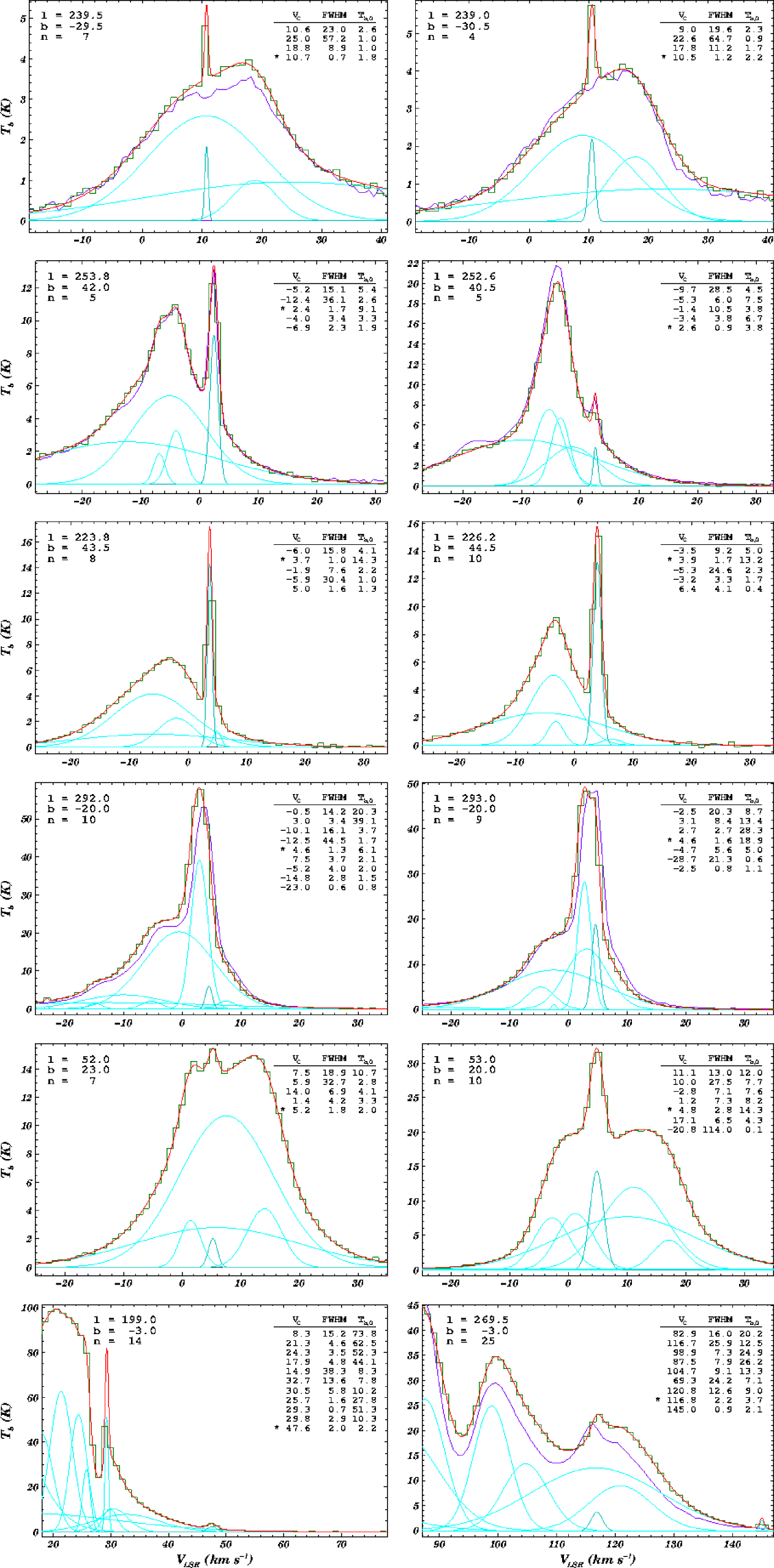
Figure 1: Examples of profile fragments with narrow components. The observed LAB profiles are plotted by green stepped lines, individual Gaussian components by turquoise thin smooth lines, and the Gaussian representations of the profiles by red thick smooth lines. The dark violet piecewise linear lines represent the GASS observations. The numerical data in the upper left corner of each panel give the Galactic coordinates and the total number of Gaussians for this profile. In the upper right corner are the parameters of Gaussians, contributing to the model profile in the velocity range of the figure. The Gaussian component, belonging to the cloud under discussion, is drawn by a thicker dark turquoise line near the center of the velocity axis of each panel and marked with an asterisk in the table of Gaussian parameters. Row 1: the cloud candidate with the narrowest average line width. Row 2: the ring cloud with the narrowest average line width. Row 3: Verschuur’s cloud A. Row 4: heavily blended components. Row 5: profiles from the comet-like structure, discussed in Sec. 3. Row 6: two clouds at higher velocities near the Galactic plane, used for Fig. 4.

As described in Haud (Hau00 (2000)), the Gaussian decomposition of the LAB profiles was adjusted so that on average once per two profiles some stronger noise peak was fitted with a Gaussian, which was then also included in the final database of the Gaussians. This approach improved the detection of weak signal features, but at the same time, in this way slightly more than $6\%$ of all Gaussians in our final database actually represent noise, and most of these components are rather narrow (in Fig. 3, discussed in greater detail later in this paper, they are concentrated around $(T_{\mathrm{b}},\mathrm{FWHM})=(0.5\leavevmode\nobreak\ \mathrm{K},0.9\leavevmode\nobreak\ \mathrm{km\,s}^{-1})$). Therefore, at first glance, it may seem that a considerable part of the cloud candidates may represent such noise features, but actually this is not the case. First of all, we have required from all cloud candidates to have a mean of $T_{\mathrm{b}}\geq 1.0\leavevmode\nobreak\ \mathrm{K}$, and this excludes most of the noise peaks from consideration. Moreover, the noise is random in its nature, and therefore, it is highly improbable that many neighboring profiles exhibit strong noise features at similar velocities. Since our cloud candidates all have similar components from at least seven neighboring sky positions, we believe that the contamination by the noise is actually negligible and may become somewhat considerable only in the case of Fig. 4, for which smaller clouds, detected at least in three neighboring sky positions, were also used.

The situation is more complicated with RFI, since they are often considerably stronger than the noise and persist during certain time periods during the observations. In the case of the LAB, the sky was observed by $5\degr\times 5\degr$ fields. If the interference existed during a considerable part of the observations of one field and remained undetected in the process of the following data reduction, we may obtain nice “clouds” of RFI. These doubts are deepened by Fig. 3 of Paper I, or the upper panel of Fig. 2 here. Especially in the southern sky, we can see some “clouds” of approximately rectangular shape and size close to $5\degr\times 5\degr$ (e.g., the “clouds” near $(l,b)=(336\degr,-70\degr)$ and $(318\degr,-62\degr)$, but also others). As described in Paper I, we applied special selection criteria to suppress such features, but it seems that these criteria have not been successful in all cases.

This confirms that not all our candidates correspond to real clouds, but from the LAB alone, it is hard to distinguish which may be real and which may be spurious. However, the RFI is often specific to a particular observation time, location, or equipment. Therefore, the best check of the situation may be obtained by observing the same sky regions at different times and locations with different equipment. Such a possibility for the southern sky is provided by the Parkes Galactic all-sky survey (GASS; McClure-Griffiths et al. McC09 (2009), the data of the second data release by Kalberla et al. Kal10 (2010) are available at http://www.astro.uni-bonn.de/hisurvey), and this check confirms that not only the rectangular “clouds” referred to above, but also some more naturally looking ones are most likely caused by RFI.

The example of the situation is given in the first row of Fig. 1. From the LAB data we found at $(l,b)=(239\degr,-31\degr)$ a “cloud” with narrow line width. The line profiles from this region exhibit a clear narrow feature at about $V_{\mathrm{LSR}}=10.7\leavevmode\nobreak\ \mathrm{km\,s}^{-1}$. Similar features are detected in nine neighboring profiles, and Fig. 1 illustrates two of them together with corresponding Gaussian decompositions. However, nothing similar was found in GASS. As a result, we must recognize that this “cloud” is most likely a spurious feature. At the same time, as we can see from the second row of Fig. 1, the reality of one ring cloud is confirmed well by the GASS data and, as discussed later, some more of them, located outside the region which is covered by the GASS, are confirmed by other independent observations (e.g., the one in the third row of Fig. 1).

Many narrow Gaussians are heavily blended by the wider ones, and in such cases, even the direct comparison of the observed profiles from the LAB and GASS may not give a conclusive result (the fourth row of Fig. 1). Such blended components may easily be the artifacts of the Gaussian decomposition, since it is well known that often the Gaussian decomposition is not unique, and several quite different solutions may approximate the observed profiles almost equally well. The decomposition provides no satisfactory means of choosing between these solutions, while other equally good or even better ones may not be found at all. Such nonuniqueness affects the heavily blended components most seriously, as in these cases even small changes in the data or in the decomposition process may lead to completely different decomposition results. Therefore, to check how prone our results are to such uncertainties, the most conclusive solution is to repeat the search of the clouds using more or less independent observations and a more or less different decomposition algorithm.

As mentioned above, in the southern sky the possibility of using independent data is offered by the GASS. For the LAB and GASS, different observing instruments (30-m dish of the Instituto Argentino de Radioastronomía and the Parkes 64 m radio telescope, respectively) and techniques (pointed observations for the LAB against on-the-fly observations in the GASS) were used. Compared to the LAB, the GASS has considerably better spatial resolution and slightly better velocity resolution and sensitivity. For the northern sky, the observations, similar to the GASS, are going on in Germany (the Effelsberg-Bonn H i Survey or EBHIS; Kerp et al. Ker11 (2011)), but the corresponding results are not yet available. Therefore, it seems interesting to decompose the GASS data and to compare the results with the decomposition of the LAB. For the northern sky we have to hope that the outcome of any future comparison of the EBHIS and LAB will in general be similar.

For decomposition, the GASS data were prepared in the HEALPix grid (Górski et al. Gor05 (2005)) with $N_{\mathrm{side}}=1024$ by P. Kalberla, and the obtained 6 655 155 profiles were decomposed with the modified version of our decomposition program into 60 349 584 Gaussians. We used the original version of the same program (Haud Hau00 (2000)) also for the decomposition of the LAB data, and therefore we cannot claim that the decomposition algorithms, which were applied to the LAB and GASS, were completely independent, but there were nevertheless important differences. First of all, the algorithms for finding the initial approximations for the decomposition of each profile were completely different. When processing the LAB, for the decomposition of a new profile the result of the earlier decomposition of one of its neighbors was used as the initial approximation. In the case of the GASS, the decomposition of each profile was started independently of all the others with only one Gaussian roughly fitting the main peak of the given profile. During the following decomposition, the weighting of the profile channels was also made differently for the LAB and GASS. In the LAB, we had just one profile for most sky positions, and therefore the dependence of the uncertainties of the channel values on the signal strength had to be estimated semitheoretically (discussed in detail in Haud Hau00 (2000)). In the GASS, typically 40 individual spectra contributed to every final resolution element. Therefore, it was possible to estimate, for every final profile, the uncertainties of all channels from the mutual deviations of the contributing profiles and from the presence of the flagged channels (Kalberla et al. Kal10 (2010)). Besides these main differences in the decomposition algorithms, there were also some others (a new path for proceeding through the survey profiles, a new definition of the neighborhood of all profiles, etc.), but their influence on the final decomposition results is probably less severe.

Owing the described differences in the decomposition processes of the LAB and GASS, it seems plausible that in ambiguous cases we will get rather different sets of Gaussians for the profiles of these two surveys, and similar Gaussians will indicate the real features, detected by both surveys. For the final comparison of the decomposition results, we decided also to repeat the cloud-finding procedure applied to the LAB Gaussians with the GASS data. We carried this procedure out in exactly the same way as for the LAB with only one exception. The HEALPix grid for $N_{\mathrm{side}}=1024$ is much denser than the grid used for the observations of the LAB, and therefore, if we would like to search in both surveys for the clouds of approximately the same sizes, the requirement on the number of neighboring sky positions with similar narrow components must be considerably increased for the GASS. From the comparison of the total number of the profiles in the LAB with the number of resolution elements in HEALPix, we concluded that seven neighboring positions in the LAB correspond to 464 positions in the GASS and considered further only the GASS clouds of at least this size.

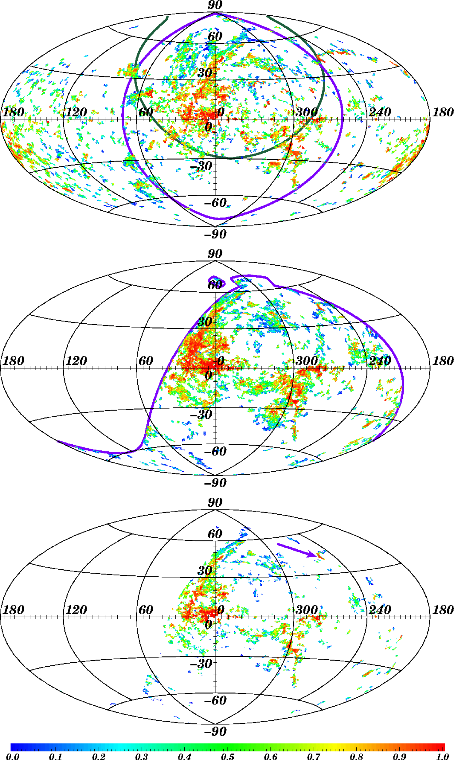
Figure 2: The NHIE clouds from the LAB (upper panel), from the GASS (middle panel), and from both (lower panel). Every Gaussian, belonging to an NHIE cloud candidate, is represented with the color, corresponding to the sequence number of this component in the ascending list of the values of $T_{\mathrm{b,0}}/\mathrm{FWHM}^{2}$ of these Gaussians. The red color corresponds to the highest values of $T_{\mathrm{b,0}}/\mathrm{FWHM}^{2}$. The numbers on the color scale below the figure denote the fractions of the length of the list. The thick lines in the upper panel indicate the location of the expanding superbubble shells S1 (dark violet) and S2 (sea green). In the middle panel, the border of the region covered by the GASS is indicated. The arrow in the lower panel points to the cloud with the narrowest lines, reliably detected in both the LAB and GASS.

The results of the comparison are presented in Fig. 2. The color of the points in this figure represents the values of the rather arbitrarily chosen parameter $T_{\mathrm{b,0}}/\mathrm{FWHM}^{2}$. The justification for this choice is that this parameter has the highest values for the strongest and narrowest components, which are the most interesting ones in the context of our discussion. However, as the actual values of the parameter are not very important, we rescaled them for every part of Fig. 2 in the following way. First, we found which clouds satisfy all our selection criteria, then we calculated $T_{\mathrm{b,0}}/\mathrm{FWHM}^{2}$ for every Gaussian of these clouds, sorted the Gaussians in ascending order of the parameter values, and colored them according to their sequence number in the ordered list. In this way, in each panel the $10\%$ of the strongest and narrowest Gaussians are drawn with red color, next $10\%$ are orange, next $10\%$ yellow, etc. The upper panel of Fig. 2 reproduces all clouds from the LAB, the middle panel is for the results from the GASS and the lowest panel represents the product of the upper two. This means that in the lowest panel only those clouds are represented that were found in both the LAB and GASS. We see that all three panels of Fig. 2 are remarkably similar and for the southern sky we may find all main features in all these panels. This is not the result that we expect if most of our narrow Gaussians are artifacts of the Gaussian decomposition of ambiguous cases of heavily blended profile features. Therefore, we conclude that despite some spurious features in the list of the cloud candidates, most of the clouds, found by us in the LAB and then found again in the GASS, are real. However, if so, we may also ask about their physical nature.

3 Narrow-line neutral hydrogen emission

When we started to search for references to objects similar to those found in our study, the results were rather scarce. The situation was clarified by the recent statement of Gibson (Gib11 (2011)): “Historically only a few NHIE features were known (Knapp & Verschuur Kna72 (1972); Goerigk et al. Goe83 (1983)), but increasingly sophisticated spectral decompositions have revealed more (Verschuur & Schmelz Ver89 (1989); Pöppel et al. Pop94 (1994); Haud Hau10 (2010))”. Of all these papers, Knapp & Verschuur (Kna72 (1972)) studied a cloud, which is also a part of the filament discussed by us in Paper I. Goerigk et al. (Goe83 (1983)) studied the Draco cloud, which we also found in our analysis, but because according to Goerigk et al. (Goe83 (1983)), its mean $\mathrm{FWHM}>4.0\leavevmode\nobreak\ \mathrm{km\,s}^{-1}$ (the velocity resolution of their data was $1.69\leavevmode\nobreak\ \mathrm{km\,s}^{-1}$) and $V_{\mathrm{LSR}}\approx-22\leavevmode\nobreak\ \mathrm{km\,s}^{-1}$, it is not among the 1 336 cloud candidates discussed in Paper I.

Verschuur & Schmelz (Ver89 (1989)) presented the results of observations of H i emission profiles in 180 directions over the northern sky and noticed that the peak in the histogram of the line-width distribution occurs at $3\leavevmode\nobreak\ \mathrm{km\,s}^{-1}$. Their observations were made with the channel bandwidth of $0.258\leavevmode\nobreak\ \mathrm{km\,s}^{-1}$. Therefore, this NHIE most likely corresponds to normal CNM (mean $\mathrm{FWHM}=3.9\pm 0.6\leavevmode\nobreak\ \mathrm{km\,s}^{-1}$ according to Haud & Kalberla Hau07 (2007)). We can also offer a similar comment on the results by Pöppel et al. (Pop94 (1994)), who made a systematic separation of the CNM from the warm neutral medium (WNM). Using the data with a velocity resolution of about $2\leavevmode\nobreak\ \mathrm{km\,s}^{-1}$, and considering only the profile peaks with $\mathrm{FWHM}\geq 6\leavevmode\nobreak\ \mathrm{km\,s}^{-1}$, they found the mean $\mathrm{FWHM}\approx 10.6\leavevmode\nobreak\ \mathrm{km\,s}^{-1}$ for the CNM and about $23.5\leavevmode\nobreak\ \mathrm{km\,s}^{-1}$ for the WNM. Therefore, their NHIE most likely corresponds already to our line-width group 2 in the thermally unstable regime (mean $\mathrm{FWHM}=11.8\pm 0.5\leavevmode\nobreak\ \mathrm{km\,s}^{-1}$; Haud & Kalberla Hau07 (2007)).

All this indicates that the notion of NHIE has so far been used almost for any H i, colder than the WNM, and our clouds are among the most narrow-lined ones of the NHIE objects discussed above. From the frequency distribution of the Gaussian widths and heights, it may even seem that these very narrow-lined H i emission (VNHIE?) clouds may belong to the population distinct from the CNM (Fig. 3, below the thick blue line). However, this conclusion is most likely an artifact of the observations and data reduction. We modeled the observations of Gaussian-shaped lines of different widths and realistic noise with a velocity channel separation typical of the LDS. After Gaussian decomposition of these “observations”, we found that all lines are statistically well reproduced by such a procedure down to the line width of about $\mathrm{FWHM}\approx 0.77\leavevmode\nobreak\ \mathrm{km\,s}^{-1}$. Below this limit the obtained widths of Gaussians become independent of the original line widths, and most decomposition results concentrate around the value of $0.77\leavevmode\nobreak\ \mathrm{km\,s}^{-1}$, with the sharp boundary of the distribution at $0.54\leavevmode\nobreak\ \mathrm{km\,s}^{-1}$. The same behavior is also observed in Fig. 3. Moreover, the frequency concentration below the thick line in Fig. 3 is also enhanced by the contamination of the survey by the radio interferences, and most of the weakest Gaussians at these widths are due to the highest noise peaks in the data, which were considered by the decomposition program as a possible signal (Haud & Kalberla Hau06 (2006)). For these reasons, we continue to use the acronym NHIE for our clouds, but at least in this paper we mean the VNHIE by it.

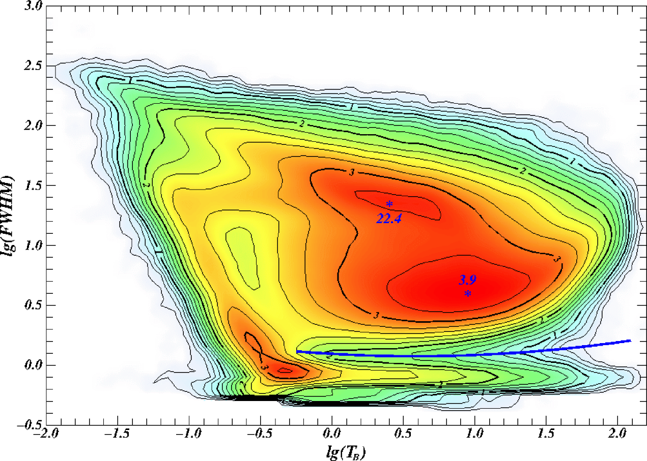
Figure 3: Frequency distribution of the parameter values in the $(\lg(T_{\mathrm{b,0}}),\lg(\mathrm{FWHM}))$ plane for all Gaussians obtained in the decomposition of the LAB. Isodensity lines are drawn on the scale of $\lg(N+1)$ with the interval of 0.2. The two main maxima, corresponding to WNM and CNM, are labeled with the values of corresponding Gaussian $\mathrm{FWHM}$. The blue thick solid line represents the selection criterion defined by Eq. 4 of Haud & Kalberla (Hau06 (2006)).

Probably the most thoroughly studied object among our clouds is the one discovered by Verschuur (Ver69 (1969)) as cloud A at $(l,b)\approx(226\degr,44\degr)$, and studied in more detail later by Verschuur & Knapp (Ver71 (1971)), Knapp & Verschuur (Kna72 (1972)), Crovisier & Kazès (Cro80 (1980)), Crovisier et al. (Cro85 (1985)), Heiles & Troland (2003b ), Meyer et al. (Mey06 (2006)), and Peek et al. (2011b ). Already in his first paper on cloud A, Verschuur (Ver69 (1969)) stated that the cloud must have a kinetic temperature $T_{\mathrm{k}}\leq 30\leavevmode\nobreak\ \mathrm{K}$. Later authors have agreed with this estimate, and recent papers explain the observed line width as a result of the kinetic temperature $20_{-8}^{+6}\leavevmode\nobreak\ \mathrm{K}$, and the one-dimensional RMS turbulent velocity of $0.37\pm 0.08\leavevmode\nobreak\ \mathrm{km\,s}^{-1}$ (Meyer et al. Mey06 (2006)). Up to now, this cloud A has contained the narrowest H i emission lines ever discovered, and it is also part of our ringlike ribbon of clouds (example profiles in the third row of Fig. 1), but it may not be the cloud with the narrowest lines in this ribbon. According to our estimates, the cloud (example profiles in the second row of Fig. 1) at the highest Galactic longitude tip of the stream may have even narrower lines. However, even now Verschuur’s cloud A presents the narrow components, which are among the strongest and most securely identifiable of all similar components discussed in this paper.

For other cloud candidates in our sample, we do not have such temperature estimates, and we even do not have enough information for obtaining them. In the Introduction we pointed out why our line-width estimates may be only the upper limits to the actual line widths. To obtain the temperatures from line widths, we must additionally know how much of the real line width is caused by the temperature and what is contributed by turbulence. We do not have this information. However, Heiles & Troland (2003b ) have established a correlation between the upper limit on the kinetic temperature, $T_{\mathrm{k,max}}$, as estimated from the fitted width of the Gaussian component and the spin temperature $T_{\mathrm{s}}$ (their Eq. 15a). From our decomposition of the LAB data we found the average line width of the Gaussians belonging to cloud A, of about $1.6\leavevmode\nobreak\ \mathrm{km\,s}^{-1}$. Using this result in the correlation and taking into account that $T_{\mathrm{k,max}}=21.86\mathrm{FWHM}^{2}$ and that for CNM the spin temperature is equal to the kinetic temperature (Heiles & Troland 2003a ; 2003b ), we obtain for this cloud $25\leavevmode\nobreak\ \mathrm{K}$. This is already within the errors of the more accurate estimate above.

At the same time, the correlation by Heiles & Troland (2003b ) was established for $T_{\mathrm{k,max}}$, estimated from the Gaussian fit of the opacity profiles, but we have used the decomposition of the emission lines. It is known from the equation of transfer that the emission line of an isolated, single, homogeneous H i cloud may be represented well by a Gaussian only when its optical depth $\tau\ll 1$. For cloud A, Verschuur & Knapp (Ver71 (1971)) already found that the shapes of the narrow lines were not a Gaussian, and they managed to fit these shapes with the values of the maximum optical depth between 1 and 2. We fitted these non-Gaussian lines with a single Gaussian, and if we disregard that the criteria of isolation and homogeneity are essentially never met, we may calculate that for the optical depths cited above, such a Gaussian fitting results in the $13-25\%$ overestimation of the width of corresponding opacity profiles. Taking this into account, we reach the temperature estimates in the range $18<T_{\mathrm{k}}<21\leavevmode\nobreak\ \mathrm{K}$, in excellent agreement with the results of Meyer et al. (Mey06 (2006)). Therefore, we expect that it is possible in this way to obtain at least crude estimates of the temperatures of all clouds in our sample.

The most interesting are the coldest clouds. The cloud candidate with the narrowest mean line width, $\mathrm{FWHM}\approx 1.18\leavevmode\nobreak\ \mathrm{km\,s}^{-1}$, in our all-sky sample is located at $(l,b)\approx(239\degr,-31\degr)$. However, as mentioned above, when discussing the first row of Fig. 1, this cloud has not been confirmed by the GASS data. The cloud with the narrowest lines, strong signal, and clear confirmation from the GASS is at $(l,b)\approx 254\degr,42\degr$ (the second row of Fig. 1, arrow in Fig. 2) and has the mean line width, $\mathrm{FWHM}\approx 1.25\leavevmode\nobreak\ \mathrm{km\,s}^{-1}$. From the correlation, established by Heiles & Troland (2003b ), this line width corresponds to the temperature $T_{\mathrm{k}}=18\leavevmode\nobreak\ \mathrm{K}$. As described above, this estimate is most likely higher than the actual kinetic temperature of the cloud, which may be somewhere around $12\leavevmode\nobreak\ \mathrm{K}$ for the $25\%$ line-width correction.

The upper limit of the temperatures of the clouds in our sample is not of special interest, since the limiting mean line width of the clouds in the sample was chosen rather arbitrarily. Nevertheless, the condition $\mathrm{FWHM}\leq 3.0\leavevmode\nobreak\ \mathrm{km\,s}^{-1}$ corresponds to $T_{\mathrm{k}}\leq 66\leavevmode\nobreak\ \mathrm{K}$ with the same comments as for the lower temperature limit. Also applying the $25\%$ line-width correction here, this temperature becomes equal to $47\leavevmode\nobreak\ \mathrm{K}$. These rough estimates from the whole-sky data are in good agreement with the more accurate results by Dickey et al. (Dic03 (2003)) for a small test field. They find that clouds with temperatures below $40\leavevmode\nobreak\ \mathrm{K}$ are common (though not as common as warmer clouds with $40-100\leavevmode\nobreak\ \mathrm{K}$), with a long tail of the distribution reaching down to temperatures below $20\leavevmode\nobreak\ \mathrm{K}$.

For the ring clouds, we also have some distance information. From our model in Paper I, it follows that the clouds of the observed part of the ring are at distances $33-63\leavevmode\nobreak\ \mathrm{pc}$ from the Sun. At these distances their linear diameters, corresponding to the largest angular separation of the observed cloud points, are in the range $0.9-6.9\leavevmode\nobreak\ \mathrm{pc}$. The total length of the ribbon of the clouds is about $66\leavevmode\nobreak\ \mathrm{pc}$. At the same time, according to our rather rough estimates, Verschuur’s cloud A is at the distance of about $34\leavevmode\nobreak\ \mathrm{pc}$ from the Sun. More recently, Peek et al. (2011b ) have found that this cloud is most likely in the distance interval of about $11.3-24.3\leavevmode\nobreak\ \mathrm{pc}$. Proceeding from this distance estimate, we may conclude that the cloud sizes in our ribbon are about $0.3-4.1\leavevmode\nobreak\ \mathrm{pc}$, and the total length of the discussed cloud complex is $21.9-47.0\leavevmode\nobreak\ \mathrm{pc}$.

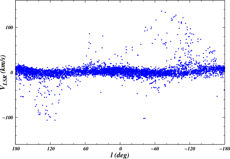
Figure 4: The $l-V$ diagram for NHIE clouds (blue dots), observed in at least three neighboring sky positions.

Information on the distances of other clouds in our whole sky sample, identified in Paper I, is practically missing. However, these objects have small line widths and, consequently, low temperatures and turbulent motions. If they have large linear dimensions, they cannot exist in such a state for a long time, and most likely they are relatively small clouds. At the same time, some of them cover up to 150 square degrees in the sky. This is only possible if they are relatively nearby.

This also agrees with the fact that all clouds of this sample have the line-of-sight velocities $|V_{\mathrm{LSR}}|\leq 15\leavevmode\nobreak\ \mathrm{km\,s}^{-1}$. At the distances beyond the local spiral arm, the differential rotation of the Galactic disk would produce higher velocities at least in some regions near the Galactic plane. However, in Paper I we also mentioned that in the initial selection 44 clouds with higher velocities were detected near the Galactic plane. These clouds were in the regions of the sky, where their velocities are naturally explained by the Galactic differential rotation. If we relax our selection criteria on the cloud sizes and velocities, we will get more clouds with higher velocities and their velocity distribution starts to resemble the usual $l-V$ diagram for the Galactic gas (Fig. 4). Unfortunately, such relaxation also increases the probability of confusion of the real NHIE clouds with the “clouds” of Gaussians, representing the traces of the removed radio interferences or observational noise. Nevertheless, we believe that we may conclude that the narrow lined clouds are detectable in the LAB at distances from some or some tens of parsecs up to several kiloparsecs. Two examples of the line profiles near the Galactic plane, containing the narrow components at higher velocities are given in the last row of Fig. 1.

Something could also be said about the locations and shapes of NHIE clouds on the basis of their sky maps (Figs. 3 and 5 of Paper I or the upper panel of Fig. 2 here). Besides the long filament of the ring clouds discussed above, the most prominent clouds or complexes seem to be four structures at approximately $l=70\degr$ and $b=-50\degr$, $-30\degr$, $15\degr$, $35\degr$, and the wide bands of clouds from $(l,b)=(20\degr,0\degr)$ to $(290\degr,70\degr)$ and from $(l,b)=(320\degr,-10\degr)$ to $(260\degr,-55\degr)$. All these apparently largest structures seem to be somehow related to expanding spherical superbubble shells S1 and S2, which are part of Loop I superbubble. These shells were introduced by Wolleben (Wol07 (2007)) to explain the results of the Dominion Radio Astrophysical Observatory Low-Resolution Polarization Survey (Wolleben et al. Wol06 (2006)) in the North Polar Spur (NPS) region.

The ring structure, modeled in Paper I, nearly perpendicularly intersects shell S2 in the direction $l=256\degr,b=43\degr$ and extends outward of this shell towards the lower Galactic longitudes. The gas stream from $(l,b)=(320\degr,-10\degr)$ to $(260\degr,-55\degr)$ is similar to the ring clouds. The stream projects onto the shell S1, and starts near the outer boundary of the shell S2, extending nearly perpendicular away from this shell. Both the ring clouds and the stream have their lowest line-of-sight velocities near S2, and the velocities increase when moving away from the shell. At the same time, the southern stream is much more irregular than the ring clouds in the northern sky. Nevertheless, both these structures may be parts of some shell structures.

Most of these other NHIE structures touch or intersect the visible boundaries of these shells as well, and the structure nearest to $l=0\degr$ resembles in its location, shape, and size the NPS, the brightest filament of Loop I, which is a large circular feature in the radio continuum sky (Quigley & Haslam Qui65 (1965); Fig. 5 of Paper I or Fig. 2 here). As the distance of the NPS from the Sun is estimated to be about $120\leavevmode\nobreak\ \mathrm{pc}$ (Bingham Bin67 (1967), Spoelstra Spo72 (1972)), the similarity of this stream to NPS may also serve as an additional hint that the NHIE clouds are probably rather nearby features. Many authors (e.g. Berkhuijsen et al. Ber71 (1971), Salter Sal83 (1983), Egger Egg95 (1995), Breitschwerdt & Avillez Bre06 (2006)) have argued that the radio loops are correlated with expanding gas and dust shells, energized by supernovas or stellar winds. They may be interesting objects where a hot gas interacts with a cool and dense H i interstellar medium (Park et al. Par07 (2007)).

Many of the NHIE features discussed here have elongated or filamentary shapes, and some of them also have an interesting internal structure. The most remarkable is the cloud complex around $(l,b)=(60\degr,15\degr)$ (Fig. 6 of Paper I). Its densest parts have the highest velocities and resemble the stream of gas, nearly perpendicular to the borders of the images of the S1 and S2 shells. This relatively dense and fast-moving gas is mostly surrounded by an envelope with lower observed line-of-sight velocities and surface densities. The most narrow-lined (the coolest?) gas is located in front of the head of this comet-like stream (in the region, closest to the S1 and S2). In central regions of the cloud, the narrow features are much stronger and slightly wider. The examples of the profile segments of the coolest gas and the gas near the center of the head of the comet-like structure are given in the fifth row of Fig. 1. The traces of a similar cometary structure may also be observed in the cloud around $(l,b)=(70\degr,-50\degr)$.

Finally, if we know the H i 21-cm line profiles, it is possible to calculate neutral hydrogen column densities for the optically thin clouds. Knowing the sizes of the clouds, it is possible to convert these column densities to spatial densities and the H i mass estimates of the clouds. Using the temperature estimates, we can determine the pressure and so on. However, we have already mentioned that at least some line profiles are seriously affected by the limited velocity resolution of the LAB data, by blending the narrow features with other H i gas, and by problems in the Gaussian decomposition. Moreover, according to Verschuur & Knapp (Ver71 (1971)), the clouds are not optically thin. Later, Peek et al. (2011b ) found that their double unsaturated Gaussian model is the best for narrow lines of cloud A. In any case, since we have fitted these lines with single Gaussians, the parameters of these Gaussians cannot be representative of the actual physical properties of the clouds. Moreover, our temperature estimates are only based on the statistical correlation between absorption line widths and kinetic temperatures which is applied to emission line widths. The distances follow from the correlation between the line widths and linear dimensions of the molecular clouds which is applied to H i clouds. Therefore, we must conclude that the obtained estimates are only very rough ones, and their combinations are even more questionable.

However, such estimates based on better data were made for Verschuur’s cloud A by Heiles & Troland (2003b ), Meyer et al. (Mey06 (2006)), and Peek et al. (2011b ). They find for this one cloud the H i column densities ranging up to $2.5\times 10^{20}\leavevmode\nobreak\ \mathrm{cm}^{-2}$, the density of $150-320\leavevmode\nobreak\ \mathrm{cm}^{-3}$, and the mass $0.235-1.07\leavevmode\nobreak\ M_{\sun}$. This cloud has been also observed in 18-cm OH and 2.6-mm CO lines, but without positive detections (Crovisier & Kazès Cro80 (1980)). From the $100\leavevmode\nobreak\ \mu\mathrm{m}$ infrared observations Peek et al. (2011b ) conclude that cloud A has either a lower-than-expected overall dust grain density or a population that has somewhat larger grains than is typical for the ISM.

4 Neutral hydrogen self-absorption

More commonly than in emission, the cold H i is identified in absorption against either a continuum source (H i continuum absorption = HICA) or other line emission (H i self-absorption = HISA). HICA is the method of choice for exploring CNM properties, because it has fewer radiative transfer unknowns (Heiles & Troland 2003b ). However, HICA sight lines are discrete and well separated in present surveys, so that individual clouds are often sampled only once, or missed entirely. Therefore, HISA is the preferred method for mapping detailed CNM structure in absorption. Moreover, HISA backgrounds are typically not as bright as HICA backgrounds, and so HISA observations are more focused on the coldest H i (Gibson Gib11 (2011)).

Neutral hydrogen self-absorption was discovered (Heeschen Hee54 (1954, 1955)) only three years after the first detection of H i emission from interstellar hydrogen in the Galactic plane (Ewen & Purcell Ewe51 (1951)). HISA was observed in H i profiles as a very narrow absorption dip of only $1-4\leavevmode\nobreak\ \mathrm{km\,s}^{-1}$ wide (Knapp Kna74 (1974)). Much of the earlier work used single-dish observations and achieved the angular resolutions of up to $3\aas@@fstack{\prime}2$ with the 1 000-foot Arecibo telescope (Baker & Burton Bak79 (1979); Bania & Lockman Ban84 (1984)). More recently, such interferometric surveys as the Canadian Galactic Plane Survey (CGPS; Taylor et al. Tay03 (2003)), Southern Galactic Plane Survey (SGPS; McClure-Griffiths et al. McC05 (2005)), and VLA Galactic Plane Survey (VGPS; Stil et al. Sti06 (2006)) have reached the angular resolutions of $1\arcmin$ and a velocity sampling around $0.82\leavevmode\nobreak\ \mathrm{km\,s}^{-1}$. These surveys have provided a wealth of data in which to look for and study the HISA phenomenon (Kavars et al. Kav05 (2005)).

From these data, the physical parameters of some HISA features have been determined. The results have been reviewed by Kavars et al. (Kav05 (2005)) and Gibson (Gib11 (2011)), among others. From these reviews and other sources, it follows that HISA features are observable around the Sun in the distance range from about $0.1\leavevmode\nobreak\ \mathrm{kpc}$ up to at least $7\leavevmode\nobreak\ \mathrm{kpc}$, that their linear dimensions are about $0.029-3.6\leavevmode\nobreak\ \mathrm{pc}$, and that the dimensions of the cloud complexes extend up to $10-110\leavevmode\nobreak\ \mathrm{pc}$ (Table 2 from Kavars et al. Kav05 (2005), excluding the clouds with only the upper limits for distances, and the Local Filament from Table 1 of Gibson et al. Gib00 (2000)). The estimated spin temperatures of HISA clouds depend on assumptions about their optical depth and the fraction of H i emission that originates behind the cloud. After considering the most probable values for these parameters, Kavars et al. (Kav05 (2005)) found that the spin temperatures of the 70 largest HISA complexes in their catalog range from 6 to $41\leavevmode\nobreak\ \mathrm{K}$.

Density and mass estimates of the clouds depend on the same assumptions, made for calculating the spin temperatures, but also on the uncertainties in the distance estimates and in the filling factor of the cold gas in the clouds. For their 70 HISA complexes, Kavars et al. (Kav05 (2005)) find that the total hydrogen density may range from 42 to $550\leavevmode\nobreak\ \mathrm{cm}^{-3}$, and the H i masses are about $3-4\,400\leavevmode\nobreak\ M_{\sun}$. Tighter constraints on the physical properties are possible for clouds that are seen to move from absorption into emission. Such an analysis for the HISA feature at $l=115\aas@@fstack{\circ}5$, $b=7\degr$, $V_{\mathrm{LSR}}=-13\leavevmode\nobreak\ \mathrm{km\,s}^{-1}$ is done by Kerton (Ker05 (2005)), for example. As a result, he reported the spin temperature $30.5<T_{\mathrm{s}}<45\leavevmode\nobreak\ \mathrm{K}$ and the optical depth $0.97<\tau<3.7$. For this cold H i feature he also estimated the column density $N=(1.0-6.9)\times 10^{20}\leavevmode\nobreak\ \mathrm{cm}^{-2}$, the number density $51-260\leavevmode\nobreak\ \mathrm{cm}^{-3}$, and the total mass of the object $M=5-48\leavevmode\nobreak\ M_{\sun}$.

To distinguish the HISA features from the gaps in the H i emission profiles, which are caused by other factors than absorption, the detected HISA features were verified in early studies by molecular or dust tracers at the same velocity and position (Knapp Kna74 (1974); Baker & Burton Bak79 (1979)). This was justified by the common presumption that HISA gas is too cold to exist without some form of molecular cooling and shielding from the interstellar radiation field (Gibson Gib11 (2011)), and it led to the conclusion that the HISA features are caused by the residual amounts of very cold H i in molecular clouds (Burton et al. Bur78 (1978); Baker & Burton Bak79 (1979); Burton & Liszt Bur81 (1981); Liszt et al. Lis81 (1981)). Later the cold H i clouds were found in which the H i distribution only in part coincides with that of CO cloud, while the fragments of cool H i are found well beyond the limit of the CO detection (Hasegawa et al. Has83 (1983); Gibson et al. Gib00 (2000); Kavars et al. Kav05 (2005)), or corresponding CO emission is missing at all (Peters & Bash Pet83 (1983, 1987)). Therefore, when the automated methods of feature identification and extraction for new large-scale Galactic plane surveys were developed, the requirement of verification by molecular or dust tracers was abandoned (Gibson et al. 2005b ; Kavars et al. Kav05 (2005)).

The results for the Galactic distribution of HISA and their relation to molecular gas are summarized by Gibson (Gib11 (2011)). He points out that weak self-absorption is found essentially in all directions where the emission background is bright enough. However, stronger HISA is clumped into complexes along spiral arms and tangent points. HISA also has a varying degree of correspondence with the CO emission. Most of the inner-Galaxy HISA has matching CO, but most outer-Galaxy HISA does not. In the SGPS only about 60% of the identified HISA clouds have a ${}^{12}\mathrm{CO}$ brightness temperature of at least $0.5\leavevmode\nobreak\ \mathrm{K}$ (Kavars et al. Kav05 (2005)), but some HISA lacking CO show far-infrared dust emission. Many HISA features have a filamentary appearance (Taylor et al. Tay03 (2003)), but there are also examples of cometary HISA clouds (see Fig. 2 in Gibson Gib11 (2011)). Hosokawa & Inutsuka (Hos07 (2007)) have found shell-like HISA features around the giant H ii regions W4 and W5. Even a more spectacular feature is the cold, dark arc of Knee & Brunt (Kne01 (2001)).

5 Infrared and submillimeter structures

With its unprecedented sensitivity and broad spectral coverage in the submm-to-mm range, the full-sky survey performed by the Planck satellite is providing an inventory of the cold clumps (CC) of the interstellar matter in the Galaxy (Planck Col. 2011b ). However, the detection method used to extract sources from the Planck data is based on the color signature of the objects. This results in the discovery of more extended cold components with more complex morphology than the sources found with methods that identify structures on the basis of surface brightness (Planck Col. 2011a ). Because the separation of NHIE objects was at least partly based on the surface brightness distribution, it is clear that comparing their properties with those of the Planck CC may be somewhat problematic. Moreover, the Planck CC are most likely a heterogeneous ensemble of objects, in which only the smallest nearby sources are probably the cold cores. Most of the others trace cold dust in larger irregular structures up to the mass of giant molecular complexes, and a small fraction of the sources in the Galactic plane may be superpositions of nearby and distant sources (Planck Col. 2011b ). Therefore, when trying to compare the properties of the Planck CC with the parameters of NHIE clouds, we focus our attention on the nearby subsample of CC (Figs. 17 and 18 of the Planck Col. 2011b ) or on the smallest regions of higher resolution observations (Table 3 of the Planck Col. 2011a ).

Table 1: Properties of cold clouds

	NHIE	HISA	Planck CC	IRDC
Complex size (pc)	$\sim 50$	$10-110$	$<20$	$<30$
Cloud size (pc)	$0.3-4.1$	$0.029-3.6$	$0.2-2.4$	$0.4-1.0$
Temperature (K)	$12-47$	$6-45$	$7-21$	$8-28$
Column density ($\times 10^{20}\leavevmode\nobreak\ \mathrm{cm}^{-2}$)	$2.5$	$1.0-6.9$	$8-160$	$50-200$
Number density ($\mathrm{cm}^{-3}$)	$150-320$	$42-550$	$5\times 10^{3}-10^{5}$	$5\times 10^{5}-3\times 10^{6}$
Mass ($M_{\sun}$)	$0.235-1.07$	$5-48$	$0.4-1\,800$	$23-300$

Whole-sky catalogs exist both for NHIE and the Planck CC, but the data do not have very good resolution, and the catalogs may contain rather heterogeneous ensembles of objects. For H i more detailed absorption observations exist (HISA). The cold structures, observed in absorption at shorter wavelengths are infrared dark clouds (IRDC). These clouds were initially discovered by the Infrared Space Observatory (ISO, Perault et al. Per96 (1996)) and the Midcourse Space Experiment (MSX, Carey et al. Car98 (1998); Egan et al. Ega98 (1998)) as dark structures against the bright mid-infrared background of the Galaxy. Later extensive catalogs of IRDC have been compiled by Simon et al. (2006a ) and Peretto & Fuller (Per09 (2009)). These clouds may be closely related to the Planck CC because fewer than 8% of the Planck clumps inside the region studied by Simon et al. (2006a ) are not directly associated with IRDC, and the Planck observations are sensitive to lower dust column densities than those of MSX (Planck Col. 2011b ). From the comparison of the physical parameters of the Planck CC and IRDC, the Planck Col. (2011a ) has proposed that in general the Planck CC population may be representative of a slightly earlier stage of the evolution of IRDC cold dense cores.

From the Planck Col. (2011a ; 2011b ) we may conclude that the Planck CC are observed in the distance range of $0.14-7.0\leavevmode\nobreak\ \mathrm{kpc}$, their linear dimensions are about $0.2-2.4\leavevmode\nobreak\ \mathrm{pc}$, and the dimensions of the cloud complexes extend up to $20\leavevmode\nobreak\ \mathrm{pc}$. The estimated color temperatures of the CC are mostly in the range of about $7-15\leavevmode\nobreak\ \mathrm{K}$, but some substructures are found to be warmer with $19-21\leavevmode\nobreak\ \mathrm{K}$. For such clumps, the presence of bright compact sources within the Planck-detected structures has been revealed (Juvela et al., Juv10 (2010)). These sources are probably very young stellar objects, still embedded in their cold surrounding cloud. The column density, number density, and the total mass estimates for the Planck CC are $(0.8-16)\times 10^{21}\leavevmode\nobreak\ \mathrm{cm}^{-2}$, $5\times 10^{3}-10^{5}\leavevmode\nobreak\ \mathrm{cm}^{-3}$, and $0.4-1\,800\leavevmode\nobreak\ M_{\sun}$, respectively.

IRDC are preferably high column-density objects at the distances up to $8.0\leavevmode\nobreak\ \mathrm{kpc}$ (Kainulainen et al. Kai11 (2011)). The typical linear size of an IRDC is about $5\leavevmode\nobreak\ \mathrm{pc}$ with some larger ones extending up to $30\leavevmode\nobreak\ \mathrm{pc}$ (Simon et al. 2006b ). IRDC usually contain smaller cores, defined as localized regions of higher extinction than the cloud’s average (Simon et al. 2006a ). These cold, compact cores have typical sizes of about $0.5\leavevmode\nobreak\ \mathrm{pc}$ (Rathborne et al. Rat06 (2006), Wilcock et al. Wil11 (2011)). Using the kinematic distances, Simon et al. (2006b ) have estimated that IRDC have typical peak column densities of $\sim 10^{22}\leavevmode\nobreak\ \mathrm{cm}^{-2}$, volume-averaged $\mathrm{H}_{2}$ densities of $\sim 5\times 10^{3}\leavevmode\nobreak\ \mathrm{cm}^{-3}$, and local thermodynamic equilibrium masses of $\sim 5\,000\leavevmode\nobreak\ M_{\sun}$. Many of the IRDC are completely opaque at wavelengths $7-100\leavevmode\nobreak\ \mu\mathrm{m}$. This lack of emission constrains the dust temperature to $<25\leavevmode\nobreak\ \mathrm{K}$. The median values of these parameters for cores are $\log[N(\mathrm{H}_{2})(\mathrm{cm}^{-2})]=22.01\pm 0.29$, $\log[n(\mathrm{H}_{2})(\mathrm{cm}^{-3})]=6.06\pm 0.39$, and $\log[M(M_{\sun})]=1.92\pm 0.55$ (Rathborne et al. Rat10 (2010)). The temperatures of the cores range from $8-11\leavevmode\nobreak\ \mathrm{K}$ at the center to $18-28\leavevmode\nobreak\ \mathrm{K}$ at the surface (Wilcock et al. Wil11 (2011)). The local temperature minima are strongly correlated with column density peaks, which in a few cases reach $10^{23}\leavevmode\nobreak\ \mathrm{cm}^{-2}$ (Peretto et al. Per10 (2010)). Many of the cores in IRDC are associated with bright $24\leavevmode\nobreak\ \mu\mathrm{m}$ emission sources, which suggests that they contain one or more embedded protostars. These active cores typically have warmer dust temperatures than the more quiescent, perhaps “pre-protostellar”, cores (Rathborne et al. Rat10 (2010)).

The distribution of the Planck CC is mostly concentrated in the Galactic plane, but some detections are also observed at high Galactic latitudes. The population is closely associated with Galactic structures, especially the molecular component: more than 95% of the clumps are associated with CO structures and about 75% are associated with an extinction greater than 1. Superimposed on the large-scale spiral structure of the Galaxy is a distribution of features known as shells, loops, etc. CC are primarily distributed on such structures (Planck Col. 2011b ). The clumps are found to be significantly elongated and embedded in filamentary or cometary large-scale structures (Planck Col. 2011a ). IRDC have been searched so far mostly in the inner Galaxy at $|l|<60\degr$ and $|b|<1\degr$. It has been found that they may represent the densest clumps within giant molecular clouds (Simon et al. 2006b ), and their distribution in the Galaxy may follow the spiral arms (Jackson et al. Jac08 (2008)).

6 Discussion

In this section we would like to compare the properties of the cold structures in the ISM, described in the previous sections, but this is not a straightforward task. Various methods are used to derive physical parameters from different kinds of observations, also resulting in a slightly different meaning of the obtained results. The observations used do not have the same angular resolution, and the observed objects are located from our local neighborhood to the outskirts of the Galaxy. Therefore, it is easy to confuse the small cores in the nearby objects with the complexes of such cores in more distant clouds or from the observations with poorer resolution. The mass and density estimates for NHIE and HISA are mostly from H i, whereas these estimates for the Planck CC and IRDC are mainly from the dust and molecular data, etc. Nevertheless, we try to concentrate on the coolest and densest structures in the objects discussed, and to compare their temperatures, sizes, densities, and masses in the hope of revealing at least some general trends. A short compilation of such data from the previous sections of this paper is given in Table 1.

If we compare NHIE and HISA, we may conclude that most of the properties of these two types of H i clouds are at least very similar. The only obvious difference is in their sky distribution. When HISA features are observed only near the Galactic plane, our NHIE clouds do not even demonstrate a remarkable concentration on this plane. It may seem that the reason for the discrepancy is that we have looked for NHIE clouds in the all-sky H i survey, but HISA features are searched for in the Galactic plane surveys, which do not extend to high latitudes. However, even in the narrow strips of these plane surveys, a strong concentration of HISA in the Galactic plane is clearly visible (e.g. Fig. 1 of Gibson et al. 2005a ).

Actually, the discrepancy in the sky distributions of HISA and NHIE clouds is a reflection of the differences in the observing conditions of these features. For self-absorption the background brightness temperature needs to be higher than the spin temperature of the absorbing gas. As most of the gas is concentrated in the Galactic plane, here we have plenty of both the foreground clouds and background H i emission. Therefore, near the Galactic plane may we expect to find a lot of HISA features. At higher latitudes the general gas density decreases quickly, and even if there are cold H i clouds, they do not have enough background emission to be observed in absorption. If at all, such cold clouds could be found there as NHIE features. An additional factor that reduces the concentration of our NHIE clouds to the Galactic plane, may be that the results of the Gaussian decomposition are more questionable in regions of more complicated H i profiles, where different features are heavily blended by each other. Therefore, very narrow Gaussian components are harder to detect at lower latitudes.

This explanation of the differences in the sky distribution of NHIE and HISA features seems to some extent also supported by the comparison of our Fig. 4 with Fig. 4 of Gibson (Gib11 (2011)). From the Gibson’s figure we can see that the strongest HISA is observed in the I and IV quadrants of the Galaxy. These quadrants correspond to the inner Galaxy with high gas densities and double-valued distance-velocity relation. This means that with the high probability for any H i cloud closer to us than the subcentral point of the sightline, there is enough background gas behind the subcentral point with the same velocity as that of the foreground cloud, so that the foreground cloud is seen in absorption against the emission of the background gas. In the outer Galaxy, the gas densities are generally lower, and the distance-velocity relation is single valued. In these regions, it is much harder to find suitable background sources for cold clouds to be observed in absorption, and therefore they are relatively rare in quadrants II and III. Here a possible source of background emission is discussed by Gibson et al. (2005a ).

If the cold H i clouds exist in the regions of the sky where they are hardly observable in absorption, they may be observable in emission as NHIE. From our Fig. 4 we see that most of the NHIE are probably rather local, since they have low line-of-sight velocities. According to Fig. 3 of Paper I or Fig. 2 here, these clouds are also located at relatively high Galactic latitudes, where the background emission is weak. The sky distribution of the small NHIE clouds with $|V_{\mathrm{LSR}}|>15\leavevmode\nobreak\ \mathrm{km\,s}^{-1}$ and $N<7$ is more strongly concentrated in the Galactic plane, and most of them have $|b|<10\degr$. However, as can be seen from Fig. 4, these objects are mostly observed in Galactic quadrants II and III, where the cold clouds are less likely observed in absorption. Therefore, the sky distributions of the HISA and NHIE are largely complementary to each other as if they have been derived from the same space distribution of objects by mutually exclusive observing conditions.

We do not see good agreement in the mass estimates of NHIE and HISA either. However, the estimate for NHIE is based on the properties of only one cloud (Verschuur’s cloud A), which is clearly a small, nearby subcondensation in a considerably larger NHIE structure (the ring, discussed in Paper I). Most of the HISA mass estimates discussed in the present paper are for large HISA complexes, but the value given in Table 1 is also derived for only one feature, whose mass may have been estimated more reliably than the masses of other clouds, because this cloud is seen in transition from absorption to emission. At the same time, the dimensions ($35\times 1.7\leavevmode\nobreak\ \mathrm{pc}$; Kerton Ker05 (2005)) of this HISA at the distance of about $1\leavevmode\nobreak\ \mathrm{kpc}$ are comparable to the full size of the observable part of our ring. If we suppose that this feature may also contain approximately the same number of subcondensations as the ring, and we divide its mass estimate by the number of assumed subcondensations, the agreement is much better. Moreover, if we compare the mass of Verschuur’s cloud A, given in Table 1, for example with the $p=f_{n}=1$ estimate for the Perseus HISA globule $M_{\mathrm{HISA}}=0.53-0.80\leavevmode\nobreak\ M_{\sun}$ (Gibson et al. 2005b ), the agreement is very good.

Finally, some cases exist where one part of the cold H i cloud is seen in self-absorption and the other part in emission. An example of this situation is the Riegel & Crutcher cold cloud, first reported as HISA by Heeschen (Hee55 (1955)) and afterwards studied by Riegel & Jennings (Rie69 (1969)), Riegel & Crutcher (Rie72 (1972)), and others. Montgomery et al. (Mon95 (1995)) reported that at longitude $l=9\aas@@fstack{\circ}87$ this cloud is detected in self-absorption between $b=-4\aas@@fstack{\circ}2$ and $+8\degr$, but outside this latitude range, the H i is observed in emission at a similar velocity. In the corresponding region of the sky, we have also detected the NHIE cloud fragments with the similar velocity. The HISA/NHIE cloud, studied by Kerton (Ker05 (2005)), has too small an angular extent to be detected by our algorithm, but nearby we have found an NHIE cloud with rather similar parameters $l=119\aas@@fstack{\circ}7$, $b=6\aas@@fstack{\circ}4$, and $V_{\mathrm{LSR}}=-10.3\leavevmode\nobreak\ \mathrm{km\,s}^{-1}$. Recently Moss et al. (Mos12 (2012)) have found a local Galactic supershell GSH 006-15+7 in which the transition from H i emission to self-absorption is observed. Fragments of this supershell seem to also be visible on our NHIE map (Fig. 5 of Paper I or Fig. 2 here). All this leads us to the conclusion that most likely HISA and NHIE features both represent the same physical class of cold H i clouds in different observing conditions.

When we compare the sky distributions of the Planck CC and IRDC with those of NHIE and HISA, we must take similar considerations into account as explained when comparing NHIE and HISA. The catalog of NHIE clouds is based on the LAB data with the gridpoint separation of about $0\aas@@fstack{\circ}5$ (Kalberla et al., Kal05 (2005)). Only the nearest clouds have large enough apparent sizes to be detected in at least seven gridpoints, as required for the catalog, and such clouds demonstrate only weak concentration in the Galactic plane. The angular resolution of the Planck observations is about $4.5\arcmin$ (Planck Col. 2011b ), the proportion of the distant, apparently smaller clumps in the detected sample is higher, and they demonstrate clearer concentration to the Galactic plane, but there are also objects at high Galactic latitudes. The surveys of HISA mostly have the resolution of $1\arcmin$ (Taylor et al. Tay03 (2003), Stil et al. Sti06 (2006)), and these observations also require the presence of bright background emission. Therefore, the observations were only made near the Galactic plane and the detections demonstrate strong concentration to it. The same is also true for IRDC, but for them the resolution of the data in sky coordinates is even better ($20\arcsec$ for MSX, up to $5\arcsec$ for the Herschel Infrared Galactic Plane Survey, and $2\arcsec$ for Spitzer satellite data). Nevertheless, all four classes of objects may be related to shock fronts in the ISM, in the spiral structure, or in shell-like structures. Also the shapes of these objects share similarities: the filamentary or cometary structures are often found.

By other parameters, the Planck CC and IRDC are most likely different from NHIE and HISA. They seem to be even colder than most of NHIE and HISA, their linear sizes are slightly smaller, and densities considerably higher than those of H i features. And, of course, when only about half of the HISA features seem to be related to the ${}^{12}\mathrm{CO}$ emission, practically all of the Planck CC and IRDC are dominated by the molecular gas.

Gibson & Taylor (Gib98 (1998)) pointed out that the complex forms of HISA exhibit morphological aspects of both HI emission wisps and molecular cloud clumps. We have already mentioned that many HISA features also appear to be associated with CO emission, though the wide range of CO brightness to HISA opacity precludes a simple relationship between the two. Gibson & Taylor (Gib98 (1998)) concluded that a possible explanation for this is that we may be seeing the actual phase transition from atomic to molecular gas brought about by the shock environment. This means that HISA features may be an intermediate evolutionary phase between the diffuse CNM and much denser molecular clumps. This assumption was later elaborated by Kavars et al. (Kav05 (2005)) and others. From the data presented in the present paper, it seems natural to suppose that NHIE clouds also represent the same intermediate phase between diffuse CNM and molecular clumps, later represented by the Planck CC and IRDC features.

The description of the discussed objects as different evolutionary stages in the conversion of diffuse CNM to molecular clumps, in which new stars may be born, seems to also be in general agreement with some theoretical calculations. We have pointed out several times that the structures described in this paper seem to have a certain relation to shock fronts in the ISM. Hosokawa & Inutsuka (Hos07 (2007)) have studied the role of an expanding H ii region in the ambient neutral medium. They have found that a shock front emerges and sweeps up the ambient CNM. The swept-up shell becomes cold ($T\sim 30\leavevmode\nobreak\ \mathrm{K}$) and dense ($n\sim 10^{3}\leavevmode\nobreak\ \mathrm{cm}^{-3}$), and $\mathrm{H}_{2}$ molecules form in the shell without CO molecules. This is just the intermediate phase between the neutral medium and molecular clouds, something like HISA or NHIE clouds in which $\mathrm{H}_{2}$ may already exist, but it is hardly detectable since CO is still largely missing. Later the shell will fragment into small clouds as a result of gravitational instability. If each fragment contracts into a dense core and increases the column density, CO molecules may form.

Molinari et al. (Mol10 (2010)) have outlined a scenario where diffuse clouds first collapse into filaments, which later fragment to cores. They point out that recent MHD numerical simulations (Banerjee et al. Ban09 (2009)) of the formation and subsequent fragmentation of filaments in the post-shock regions of large H i converging flows or in the context of helical magnetic fields (Fiege & Pudritz Fie00 (2000)) are in good agreement with the first results from the Hi-GAL survey on the core-hosting filaments, as well as with the mass regime of the cores being formed.

From the data presented in this paper, only the comparison of the masses of NHIE and HISA clouds with those of the Planck CC and IRDC cores may be somewhat disturbing. The estimates for the Planck CC and IRDC seem to be considerably higher than those for NHIE and HISA. However, we must consider at least two circumstances. First of all, the estimates for NHIE and HISA are mostly based only on H i, and so the possible contribution of the molecular gas remains largely unknown. Moreover, the cores of IRDC (and recalling their correlation with the Planck CC, also the latter) are considered as the places of high-mass star formation (Rathborne et al. Rat06 (2006)). The earliest phase of isolated low-mass star formation occurs within Bok globules (Rathborne et al. Rat10 (2010)). Viewed against background stars, Bok globules are identified as isolated, well-defined patches of optical obscuration (Bok & Reilly Bok47 (1947)). The cores of Bok globules are typically small ($\sim 0.05\leavevmode\nobreak\ \mathrm{pc}$) and dense ($10^{5}-10^{6}\leavevmode\nobreak\ \mathrm{cm}^{-3}$), with low temperatures ($\sim 10\leavevmode\nobreak\ \mathrm{K}$) and low masses ($0.5-5\leavevmode\nobreak\ M_{\sun}$; e.g., Myers & Benson Mye83 (1983); Ward-Thompson et al. War94 (1994)). Many of these low-mass star-forming regions are nearby, as most likely are also our NHIE clouds, and their masses are of the same order of magnitude as the mass estimate of Verschuur’s cloud A.

7 Conclusions

In this paper, we have argued that the Gaussian decomposition enables us to separate narrow line components from the LAB H i 21-cm line database and to compile a list of candidates of the NHIE clouds. To exclude artificial clouds, caused by RFI, non-uniqueness of the Gaussian decomposition in heavily blended cases, and the observational noise, we used the comparison of the LAB results with those obtained from the GASS in the southern sky. The obtained lists of NHIE cloud candidates for the LAB and GASS are available on request from the author (urmas@aai.ee). Then we reviewed the sizes, gas temperatures, column and number densities, and masses for NHIE and HISA clouds and for the Planck CC and IRDC. We also discussed the distribution of these clouds in the Galaxy, their basic shapes, and composition. From this discussion we draw the following conclusions

• The LAB Survey enables us to compile the low-resolution all-sky catalog of NHIE cloud candidates.

• NHIE objects share the physical properties of HISA clouds and may therefore be the same type of clouds as HISA, but in different observing conditions. In some respects, these clouds resemble the diffuse CNM, but NHIE and HISA are denser and colder.

• The Planck CC and IRDC are even colder and denser, and they contain more molecular gas than NHIE and HISA clouds, but by their distribution in the Galaxy and shapes they still resemble NHIE and HISA features.

• As proposed by Gibson & Taylor (Gib98 (1998)) and Kavars et al. (Kav05 (2005)) for HISA features, NHIE clouds may also be an intermediate phase between the diffuse cold neutral medium and molecular clumps, represented by the Planck CC and IRDC or Bok globules for the nearby, less massive clumps.

To obtain more detailed whole-sky information on the NHIE clouds, new large-scale H i 21-cm line surveys with better angular and velocity resolution than that of the LAB are needed. Unfortunately, the next generation whole-sky surveys, such as the GASS and EBHIS, offer better angular resolution than the LAB, but the velocity resolution is essentially the same. Both resolutions are considerably better in GALFA-H i (the Galactic Arecibo L-band feed array H i; Peek et al. 2011a ) survey, but it can cover only about a $39\degr$ wide strip across the sky.

- (1) Bajaja, E., Arnal, E. M., Larrarte, J. J., et al. 2005, A&A, 440, 767
- (2) Baker, P. L., & Burton, W. B. 1979, A&AS, 35, 129
- (3) Banerjee, R., Vázquez-Semadeni, E., Hennebelle, P., & Klessen, R. S. 2009, MNRAS, 398, 1082
- (4) Bania, T. M., & Lockman, F. J. 1984, ApJS, 54, 513
- (5) Berkhuijsen, E. M., Haslam, C. G. T., & Salter, C. J. 1971, A&A, 14, 252
- (6) Bingham, R. G. 1967, MNRAS, 137, 157
- (7) Bok, B. J., & Reilly, E. F. 1947, ApJ, 105, 255
- (8) Breitschwerdt, D., & de Avillez, M. A. 2006, A&A, 452, L1
- (9) Burton, W. B., & Liszt, H. S. 1981, in IAU Symp. 94, Origin of Cosmic Rays, ed. G. Setti, G. Spada & A. W. Wolfendale, 227
- (10) Burton, W. B., Liszt, H. S., & Baker, P. L. 1978, ApJ, 219, 67
- (11) Carey, S., Clark, F., Egan, M., et al. 1998, ApJ, 508, 721
- (12) Crovisier, J., & Kazès, I. 1980, A&A, 88, 329
- (13) Crovisier, J., Dickey, J. M., & Kazès, I. 1985, A&A, 149, 209
- (14) Dickey, J. M., McClure-Griffiths, N. M., Gaensler, B. M., & Green, A. J. 2003, ApJ, 585, 801
- (15) Egan, M., Shipman, R., Price, S., et al. 1998, ApJ, 494, 199
- (16) Egger, R. J. 1995, in ASP Conf. Ser. 80, The Physics of the Interstellar Medium and the Intergalactic Medium, ed. A. Ferrara et al., 45
- (17) Ewen, H. I., & Purcell, E. M. 1951, Nature, 168, 356
- (18) Fiege, J. D., & Pudritz, R. E. 2000, MNRAS, 311, 105
- (19) Gibson, S. J. 2011, in ASP Conf. Ser. 438, The Dynamic Interstellar Medium: A Celebration of the Canadian Galactic Plane Survey, ed. R. Kothes, T. L. Landecker, & A. G. Willis, 111
- (20) Gibson, S. J., & Taylor, A. R. 1998, BAAS, 30, 1341
- (21) Gibson, S. J., Taylor, A. R., Higgs, L. A., & Dewdney, P. E. 2000, ApJ, 540, 851
- (22) Gibson, S. J., Taylor, A. R., Higgs, L. A., Brunt, C. M., & Dewdney, P. E. 2005a, ApJ, 626, 195
- (23) Gibson, S. J., Taylor, A. R., Higgs, L. A., Brunt, C. M., & Dewdney, P. E. 2005b, ApJ, 626, 214
- (24) Goerigk, W., Mebold, U., Reif, K., Kalberla, P. M. W., & Velden, L. 1983, A&A, 120, 63
- (25) Górski, K. M., Hivon, E., Banday, A. J., et al. 2005, ApJ, 622, 759
- (26) Hartmann, D., & Burton, W. B. 1997, Atlas of Galactic Neutral Hydrogen, Cambridge University Press
- (27) Hasegawa, T., Sato, F., & Fukui, Y. 1983, AJ, 88, 658
- (28) Haud, U. 2000, A&A, 364, 83
- (29) Haud, U., & Kalberla, P. M. W. 2006, Balt. Astron., 15, 413
- (30) Haud, U., & Kalberla, P. M. W. 2007, A&A, 466, 555
- (31) Haud, U. 2008, A&A, 483, 469
- (32) Haud, U. 2010, arXiv:1001.4155v1 (Paper I)
- (33) Heeschen, D. S. 1954, AJ, 59, 324
- (34) Heeschen, D. S. 1955, ApJ, 121, 569
- (35) Heiles, C., & Troland, T. H. 2003a, ApJS, 145, 329
- (36) Heiles, C., & Troland, T. H. 2003b, ApJ, 586, 1067
- (37) Hosokawa, T., & Inutsuka, S-I. 2007, ApJ, 664, 363
- (38) Jackson, J. M., Finn, S. C., Rathborne, J. M., & Chambers, E. T. 2008, ApJ, 680, 349
- (39) Juvela, M., Ristorcelli, I., Montier, L. A., et al. 2010, A&A, 518, L93
- (40) Kainulainen, J., Alves, J., Beuther, H., Henning, T., & Schuller, F. 2011, A&A, 536, A48
- (41) Kalberla, P. M. W., Burton, W. B., Hartmann, D., et al. 2005, A&A, 440, 775
- (42) Kalberla, P. M. W., McClure-Griffith, N. M., Pisano, D. J., et al. 2010, A&A, 521, A17
- (43) Kavars, D. W., Dickey. J. M., McClure-Griffiths, N. M., Gaensler, B. M., & Green, A. J. 2005, ApJ, 626, 887
- (44) Kerp, J., Winkel, B., Bekhti, B. N., Fl er, L., & Kalberla, P. M. W. 2011, Astron. Nachr., 332, 637
- (45) Kerton, C. R. 2005, ApJ, 623, 235
- (46) Knapp, G. R. 1974, AJ, 79, 527
- (47) Knapp, G. R., & Verschuur, G. L. 1972, AJ, 77, 717
- (48) Knee, L. B. G., & Brunt, C. M. 2001, Nature, 412, 308
- (49) Liszt, H. S., Burton, W. B., & Bania, T. M. 1981, ApJ, 246, 74
- (50) McClure-Griffiths, N. M., Dickey, J. M., Gaensler, A. J., et al. 2005, ApJS, 158, 178
- (51) McClure-Griffiths, N. M., Pisano, D. J., Calabretta, M. R., et al. 2009, ApJS, 181, 398
- (52) Meyer, D. M., Lauroesch, J. T., Heiles, C., Peek, J. E. G., & Engelhorn, K. 2006, ApJ, 650, 67
- (53) Molinari, S., Swinyard, B., Bally, J., et al. 2010, A&A, 518, L100
- (54) Montgomery, A. S., Bates, B., & Davies, R. D. 1995, MNRAS, 273, 449
- (55) Moss, V. A., McClure-Griffiths, N. M., Braun, R., Hill, A. S., & Madsen, G. J. 2012, arXiv:1201.2700v1 [astro-ph.GA]
- (56) Myers, P. C., & Benson, P. J. 1983, ApJ, 266, 309
- (57) Park, J.-W., Min, K.-W., Seon, K.-I., et al. 2007, ApJ, 665, 39
- (58) Peek, J. E. G., Heiles, C., Douglas, K. A., et al. 2011a, ApJS, 194, 20
- (59) Peek, J. E. G., Heiles, C., Peek, K. M. G., Meyer, D. M., & Lauroesch, J. T. 2011b, ApJ, 735, 129
- (60) Perault, M., Omont, A., Simon, G., et al. 1996, A&A, 315, 165
- (61) Peretto, N., & Fuller, G. A. 2009, A&A, 505, 405
- (62) Peretto, N., Fuller, G. A., Plume, R., et al. 2010, A&A, 518, L98
- (63) Peters, W. L., & Bash, F. N. 1983, PASA, 5, 224
- (64) Peters, W. L., & Bash, F. N. 1987, ApJ, 317, 646
- (65) Planck Collaboration 2011a, A&A, 536, A22
- (66) Planck Collaboration 2011b, A&A, 536, A23
- (67) Pöppel, W. G. L., Marronetti, P., & Benaglia, P. 1994, A&A, 877, 601
- (68) Quigley, M. J. S., & Haslam, C. G. T. 1965, Nature, 208, 741
- (69) Rathborne, J. M., Jackson, J. M., & Simon, R. 2006, ApJ, 641, 389
- (70) Rathborne, J. M., Jackson, J. M., Chambers, E. T., et al. 2010, ApJ, 715, 310
- (71) Riegel, K. W., & Crutcher, R. M. 1972, A&A, 18, 55
- (72) Riegel, K. W., & Jennings, M. C. 1969, ApJ, 157, 563
- (73) Salter, C. J. 1983, Bull. astr. Inst. India, 11, 1
- (74) Simon, R., Jackson, J. M., Rathborne, J. M., & Chambers, E. T. 2006a, ApJ, 639, 227
- (75) Simon, R., Rathborne, J. M., Shah, R. Y., Jackson, J. M., & Chambers, E. T. 2006b, ApJ, 653, 1325
- (76) Spoelstra, T. A. Th. 1972, A&A, 21, 61
- (77) Taylor, A. R., Gibson, S. J., Peracaula, M., et al. 2003, ApJ, 125, 3145
- (78) Stil, J. M., Taylor, A. R., Dickey, J. M., et al. 2006, ApJ, 132, 1158
- (79) Verschuur, G. L. 1969, ApL, 4, 85
- (80) Verschuur, G. L., & Knapp, G. R. 1971, AJ, 76, 403
- (81) Verschuur, G. L., & Schmelz, J. T. 1989, AJ, 98, 267
- (82) Ward-Thompson, D., Scott, P. F., Hills, R. E., & Andre, P. 1994, MNRAS, 268, 276
- (83) Wilcock, L. A., Kirk, J. M., Stamatellos, D., et al. 2011, A&A, 526, A159
- (84) Wolleben, M. 2007, ApJ, 664, 349
- (85) Wolleben, M., Landecker, T. L, Reich, W., & Wielebinski, R. 2006, A&A, 448, 411