A Directional Gradient-Curvature Method for Gap Filling of Gridded Environmental Spatial Data with Potentially Anisotropic Correlations

Abstract

We introduce the Directional Gradient-Curvature (DGC) method, a novel approach for filling gaps in gridded environmental data. DGC is based on an objective function that measures the distance between the directionally segregated normalized squared gradient and curvature energies of the sample and entire domain data. DGC employs data-conditioned simulations, which sample the local minima configuration space of the objective function instead of the full conditional probability density function. Anisotropy and non-stationarity can be captured by the local constraints and the direction-dependent global constraints. DGC is computationally efficient and requires minimal user input, making it suitable for automated processing of large (e.g., remotely sensed) spatial data sets. Various effects are investigated on synthetic data. The gap-filling performance of DGC is assessed in comparison with established classification and interpolation methods using synthetic and real satellite data, including a skewed distribution of daily column ozone values. It is shown that DGC is competitive in terms of cross validation performance.

url]http://www.mred.tuc.gr/home/hristopoulos/dionisi.htm

1 Introduction

Atmospheric data, whether they are obtained by means of ground or remote sensing methods, often include data gaps. Such gaps arise due to different reasons, e.g. incomplete time series, spatial irregularities of sampling pattern, equipment limitations or sensor malfunctions (Jun & Stein,, 2004; Lehman et al.,, 2004; Albert et al.,, 2012; Bechle et al.,, 2013). For example, remote sensing images may include obscured areas due to cloud cover, whereas gaps also appear between satellite paths where there is no coverage for a specific period (Emili et al.,, 2011). The impact of missing data on the estimate of statistical averages and trends can be significant (Sickles & Shadwick,, 2007). There is an interest in the development of new methods for filling gaps in atmospheric data and their comparison with existing imputation methods (Junninen et al.,, 2004). Particularly for frequently collected, massive remotely sensed data, the efficient filling of the gaps is a challenging task. Traditional geostatistical interpolation methods such as kriging, e.g. (Wackernagel,, 2003), can be impractical due to high computational complexity, restriction to Gaussian data, as well as various subjective choices in variogram modeling and interpolation search radius (Diggle & Ribeiro,, 2007). In particular, computationally efficient methods are needed for filling gaps in very large data sets (Cressie,, 2008; Hartman & Hössjer,, 2008).

In the following, we consider a set of sampling points $G_{s}=\{\vec{s}_{i},\,i=1,\ldots,N\}$, where $\vec{s}_{i}=(x_{i},y_{i})\in{\mathbb{R}}^{2}$. The points are scattered on a rectangular grid $\tilde{G}$ of size $N_{G}=L_{x}\times L_{y}$, where $L_{x}$ and $L_{y}$ are respectively the horizontal and vertical dimensions of the rectangle (in terms of the unit length), such that $N_{G}>N$. Let $G_{p}=\{\vec{s}_{p},p=1,\ldots,P\}$ be the set of prediction points, representing locations of missing values, such that $\tilde{G}=G_{s}\cup G_{p}$. The data, ${\bf Z}(G_{s})=\{z_{i},\forall\vec{s}_{i}\in G_{s}\},$ are considered as a realization of the continuous random field $Z({\vec{s}_{i}})$. To reduce the dimensionality of the configuration space, we discretize the continuously valued field. For applications that do not require high resolution, e.g. environmental monitoring and risk management, ${\bf Z}(G_{s})$ can be discretized into a small (e.g., eight) number $N_{c}$ of levels (classes). Continuous distributions are obtained at the limit $N_{c}\rightarrow\infty$. In the current study, the spatial prediction of missing values is posed as a spatial classification problem for ranked numerical data. Continuous interpolation is approximated by considering an arbitrarily high number of levels.

The discretization classes ${\mathcal{C}}_{q},\,q=1,\ldots,N_{c}$ correspond to the intervals ${\mathcal{C}}_{q}=(t_{q},t_{q+1}]$ for $q=2,\ldots,N_{c}-1$, ${\mathcal{C}}_{1}=(-\infty,t_{2}],$ and ${\mathcal{C}}_{N_{c}}=(t_{N_{c}},\infty).$ The classes are defined with respect to threshold levels $t_{k},\,k=2,\ldots,N_{c}$. All the classes have a uniform width except ${\mathcal{C}}_{1}$ and ${\mathcal{C}}_{N_{c}}$ which extend to negative and positive infinity respectively, to include values outside the observed interval $[z_{\min},z_{\max}]$. More general class definitions can be investigated. The class identity field $I(\vec{s})$ takes integer values $q=1,\ldots,N_{c}$ that represent the respective class index. In particular, $I(\vec{s_{i}})=q$ implies that $z_{i}\in{\mathcal{C}}_{q}.$ The prediction problem is equivalent to assigning a class label at each point in $G_{p}$. A map of the process $Z$ can be generated consisting of equivalent-class (isolevel) contours.

2 The Directional Gradient-Curvature Model

The Directional Gradient-Curvature (DGC) model is inspired by Spartan spatial random fields (SSRF) (Hristopulos,, 2003), which are based on short-range interactions between the field values. The SSRF model is parametric and represents stationary, continuous and isotropic Gaussian random fields. To relax these assumptions, we introduce an almost non-parametric approach that aims at matching short-range correlations in $G_{s}$ with those of $\tilde{G}$. This idea was recently successfully applied to spatial random fields still assuming spatial isotropy (Žukovič & Hristopulos,, 2012). The present model extends this approach by relaxing even the isotropic assumption through incorporating anisotropic dependence. In particular, the correlations used in DGC represent the normalized squared gradient and curvature energies of the discretized class identity field along different directions. Let $a_{n}$ be the lattice step in direction $\vec{e}_{n}$. The local square gradient and curvature terms in each of the $d$ directions used are given by

$$G_{n}(I;\vec{s}_{i})=\frac{\left[I(\vec{s_{i}}+a_{n}\vec{e}_{n})-I(\vec{s_{i}})\right]^{2}}{a_{n}^{2}},\quad n=1,\ldots,d$$ (1)

$$C_{n}(I;\vec{s}_{i})=\frac{\left[I(\vec{s_{i}}+a_{n}\vec{e}_{n})+I(\vec{s_{i}}-a_{n}\vec{e}_{n})-2I(\vec{s_{i}})\right]^{2}}{a_{n}^{4}},\quad n=1,\ldots,d.$$ (2)

The normalized squared gradient, $\overline{G}_{n}({\bf I}_{g}),$ and curvature, $\overline{C}_{n}({\bf I}_{g})$ energies in a direction $\vec{e}_{n}$, are defined as averages of the above over the grid $\tilde{G}$. ${\bf I}_{g}=[I(\vec{s}_{1})\ldots I(\vec{s}_{N_{G}})]\,\forall\,\vec{s}_{i}\in\tilde{G},$ represents the values of the class identity field on the entire grid, ${\bf I}_{p}=[I(\vec{s}_{1})\ldots I(\vec{s}_{P})]\,\forall\,\vec{s}_{i}\in G_{p},$ is the class field at the prediction sites, and ${\bf I}_{s}=[I(\vec{s}_{1})\ldots I(\vec{s}_{N})]\,\forall\,\vec{s}_{i}\in G_{s}$ are the class identity values at the sampling sites. The matching of the gradient and curvature constraints on $G_{s}$ and $\tilde{G}$ is based on the following objective functional:

$$U({\bf I}_{p}|{\bf I}_{s}) =\sum\limits_{n=1}^{d}\,\left[w_{1}\,\phi\big{(}\overline{G}_{n}({\bf I}_{g}),\overline{G}_{n}({\bf I}_{s})\big{)}+w_{2}\,\phi\big{(}\overline{C}_{n}({\bf I}_{g}),\overline{C}_{n}({\bf I}_{s})\big{)}\right],$$ (3)

$$\phi(x,x^{\prime}) =\left\{\begin{array}[]{ll}\left(1-x/x^{\prime}\right)^{2},&x^{\prime}\neq 0\\ x^{2},&x^{\prime}=0.\end{array}\right.$$ (6)

In the above, $w=(w_{1},w_{2})$ represent gradient and curvature weights ($w_{1},w_{2}\geq 0$, $w_{1}+w_{2}=1$), and $d$ is the number of the directions used. We use (6) to measure the deviation between the $G_{s}-$ and $\tilde{G}-$based values instead of $\phi=(x-x^{\prime})^{2}$, because the gradient and curvature can have very different magnitudes, depending on the units used; this means that one term may dominate in the optimization. By using normalized constraints we compensate for the possible disparity of magnitudes between gradient and curvature. If one of the sample quantities is zero, the second line of (6) is used to avoid a singular denominator.

We select $w=(0.5,0.5)$ and $d=4$, representing four directions with the following angles (with respect to the positive x-axis): $0^{\circ}$, $45^{\circ}$, $90^{\circ}$, and $135^{\circ}$. Given the above, the classification problem is equivalent to determining the optimal configuration $\hat{{\bf I}}_{p}$ that corresponds to the minimum of (3):

$$\hat{{\bf I}}_{p}=\operatorname*{arg\,min}_{{\bf I}_{p}}U({\bf I}_{p}|{\bf I}_{s}).$$ (7)

The optimization of (3) is conducted numerically. The choice of the initial configuration is important to obtain a reliable, fast and automatic algorithm: it should prevent the optimization from getting trapped in poor local minima and minimize the relaxation path in configuration space to the equilibrium, and it should also minimize the need for user intervention. The sampling points retain their values ${\bf I}_{s}$. Assuming a certain degree of spatial continuity, common in geospatial data sets, the initial state of ${\bf I}_{p}$ is determined based on the sample states in the immediate neighborhood of the individual prediction points. The neighborhood of ${\vec{s}_{p}}$ is determined by an $m\times m$ stencil ($m=2l+1$) centered at ${\vec{s}_{p}}$. Then, the initial value at a prediction point is assigned by majority rule, based on the prevailing value of its sample neighbors inside the stencil. The stencil size is chosen automatically, reflecting the local sampling density and the distribution of class identity values. Namely, it is adaptively set to the smallest size that contains a finite number of sampling points with a prevailing value. If no majority is reached up to some neighborhood size $m_{\max}\times m_{\max}$, the initial value is assigned (i) randomly from the range of the labels with tie votes or (ii) from the entire range of labels $1,...,N_{c}$, if majority is not reached due to absence of sampling points within the maximum stencil. The above method of initial state assignment will be referred to as majority rule with adaptable stencil size (MRASS).

The updating of class identity states on $G_{p}$ uses the “greedy” Monte Carlo (MC) method (Papadimitriou & Steiglitz,, 1982), which unconditionally accepts a new state if the latter lowers the cost function. The greedy MC algorithm may cause the termination of the DGC algorithm at local minima of the objective function (3). Targeting exclusively global minima (e.g. by simulated annealing) unduly emphasizes exact matching of the energies on the entire domain with those in the sample domain; however, the latter are subject to sampling fluctuations and measurement errors.

The algorithm performs a random walk through the grid $G_{p}$. It terminates if $P$ consecutive update trials do not produce a single successful update. If the computational budget is a concern, the algorithm can terminate when a pre-specified maximum number of Monte Carlo steps is exceeded. In either case, the generated realization is accepted only if the residual value of the cost function is below a user-defined tolerance level $tol$. Otherwise, the realization is rejected and a new one is generated. The algorithm generates $M$ different realizations. The median values from all the accepted realizations at each missing-value point represent the prediction of the algorithm. Associated confidence intervals are also derived.

The main steps of the procedure described above are summarized by means of the following algorithm.

1. Define the number of realizations $M$, the number of classes $N_{c}$, the maximum stencil size $m_{\max}$, the residual cost function tolerance $tol$ and the maximum number of Monte Carlo steps $i_{\max}$ (optional).

2. Discretize ${\bf Z}(G_{s})$ to obtain the sample class identity field ${\bf I}_{s}.$

3. Calculate the directional sample energies $\overline{G}_{n}({\bf I}_{s})$, $\overline{C}_{n}({\bf I}_{s})$, $n=1,\ldots,d.$

4. Initialize the simulated realization index $j=1$.

5. while $j\leq M$ repeat the following steps:

   1. Assign initial values $\hat{\bf I}_{p}^{(0)}$ to the prediction points in $G_{p}$ based on MRASS.

   2. Calculate the initial energy values $\overline{G}_{n}({\bf I}^{(0)}_{g})$, $\overline{C}_{n}({\bf I}^{(0)}_{g})$, $n=1,\ldots,d$, and the objective function $U^{(0)}=U(\hat{\bf I}^{(0)}_{p}|{\bf I}_{s}).$

   3. Initialize the simulated state index $i=0,$ and the rejected states index $i_{r}=0$.

   4. while $(i_{r}<P)\wedge(i\leq i_{\max})$ repeat the following updating steps:

      1. Generate a new state $\hat{\bf I}_{p}^{(i+1)}$ by randomly, i.e., with probability 0.5, adding $\pm 1$ to the state $\hat{{\bf I}}_{p}^{(i)}$, maintaining the condition $1\leq\hat{I}^{(i+1)}(\vec{s}_{j})\leq N_{c},\;\forall\vec{s}_{j}\in G_{p}.$

      2. Calculate $\overline{G}_{n}({\bf I}^{(i+1)}_{g})$, $\overline{C}_{n}({\bf I}^{(i+1)}_{g})$, $n=1,\ldots,d.$

      3. Calculate $U^{(i+1)}=U(\hat{{\bf I}}^{(i+1)}_{p}|{\bf I}_{s}).$

      4. If $U^{(i+1)}<U^{(i)}$ accept the new state $\hat{{\bf I}}^{(i+1)}_{p}$; $i_{r}\rightarrow 0$;
         else $\hat{{\bf I}}^{(i+1)}_{p}=\hat{{\bf I}}^{(i)}_{p}$; $U^{(i+1)}=U^{(i)}$; $i_{r}\rightarrow i_{r}+1$; end.

      5. $i\rightarrow i+1$;

      end while

   5. If $U^{(i)}<tol$ store the realization $\hat{{\bf I}}^{*}_{p}(j)=\hat{{\bf I}}^{(i)}_{p}$; $j=j+1$;
      else return to 5 (a); end.

   end while

6. Evaluate the statistics from the realizations $\hat{{\bf I}}^{*}_{p}(j),\ j=1,...,M.$

The DGC method lies between interpolation and conditional simulation. Interpolation methods provide a single optimal configuration of the missing values, e.g., kriging is based on the minimization of the mean square error. Conditional simulation based on Markov Chain Monte Carlo methods aims to sample the entire configuration space and reconstruct the joint conditional probability density function of the missing data. DGC on the other hand samples the configuration space that corresponds to local minima of the objective function. Since DGC returns multiple realizations, we can characterize it as a stochastic method. However, in DGC the sampling of the configuration space is restricted to the subspace of local minima. The afforded dimensionality reduction is responsible for the computational efficiency of the method.

3 DGC validation methodology

In this section we conduct numerical experiments, in which a portion of the data is set aside to be used for validation of the classification/interpolation algorithms tested. The performance of DGC is evaluated by calculating the misclassification rate $F^{*}=1/P\sum_{\vec{s}_{p}\in G_{p}}\left[1-\delta\big{(}I(\vec{s}_{p}),\hat{I}(\vec{s}_{p})\big{)}\right]$, where $I(\vec{s}_{p})$ is the true class identity value at the validation points, $\hat{I}(\vec{s}_{p})$ is the classification estimate and $\delta(I,I^{\prime})=1$ if $I=I^{\prime}$, $\delta(I,I^{\prime})=0$ if $I\neq I^{\prime}$. The gap-filling of DGC is compared with the $k$-nearest neighbor (KNN) (Dasarathy,, 1991) and fuzzy $k$-nearest neighbor (FKNN) (Keller et al.,, 1985) classification algorithms. We chose the $k$ values that minimize the cross validation errors to obtain the lowest achievable errors by KNN and FKNN. The KNN and FKNN algorithms are applied using the Matlab®  function fknn (Akbas,, 2007).

The interpolation performance is compared with the inverse distance weighted (ID) (Shepard,, 1968), nearest neighbors (NN), bilinear (BL), bicubic (BC), and biharmonic spline (BS)(Sandwell,, 1987) methods. For the Gaussian synthetic data we also include the ordinary kriging (OK) method (Wackernagel,, 2003). Given the Gaussian distribution and knowledge of the covariance parameters, OK provides optimal predictions and thus also a standard for comparing DGC estimates. The NN, BL, BC and BS interpolation algorithms were implemented by means of the Matlab®  function griddata. For ID we used the Matlab®  function fillnans (Howat,, 2007). Finally, for OK we used the routines available in the Matlab®  library vebyk (Sidler,, 2009).

Let $\hat{Z}(\vec{s}_{p})$ be the estimate of the continuous field calculated from the back transformation

$$\hat{Z}(\vec{s}_{p})=[t_{\hat{I}_{Z}(\vec{s}_{p})}+t_{\hat{I}_{Z}(\vec{s}_{p})+1}]/2,\ p=1,\ldots,P.$$ (8)

If $Z(\vec{s}_{p})$ is the true value at $\vec{s}_{p}$ the estimation error is $\epsilon(\vec{s}_{p})=Z(\vec{s}_{p})-\hat{Z}(\vec{s}_{p}).$ For $N_{c}>>1$ we calculate the following prediction errors: average absolute error

$${\rm AAE}=(1/P)\sum_{\vec{s}_{p}\in G_{p}}|\epsilon(\vec{s}_{p})|,$$ (9)

average relative error

$${\rm ARE}=(1/P)\sum_{\vec{s}_{p}\in G_{p}}\epsilon(\vec{s}_{p})/Z(\vec{s}_{p}),$$ (10)

average absolute relative error

$${\rm AARE}=(1/P)\sum_{\vec{s}_{p}\in G_{p}}|\epsilon(\vec{s}_{p})|/Z(\vec{s}_{p}),$$ (11)

root average squared error

$${\rm RASE}=\sqrt{\sum_{\vec{s}_{p}\in G_{p}}(1/P)\,\epsilon^{2}(\vec{s}_{p})},$$ (12)

and linear correlation coefficient $R$.

If $S$ sample configurations are considered, the mean values of the validation measures (i.e., the MAAE, MARE, MAARE, MRASE, and MR) are calculated by averaging over the sample configurations. To focus on the local performance of DGC, we use the respective “local” errors, i.e., MAE, MRE, MARE, and RMSE, in which the spatial average is replaced by the mean over predictions obtained from $M$ different simulations. Furthermore, we record the optimization CPU time, $T_{cpu}$, and the number of Monte Carlo steps (MCS).

The computations are performed in Matlab® programming environment on a desktop computer with 3.25 GB RAM and an Intel®Core™2 Quad CPU Q9650 processor with an 3 GHz clock.

4 Results

4.1 Synthetic Data

DGC performance is first studied on synthetic data sampled on regular grids. The data are simulated from the Gaussian random field $Z\sim N(m=50,\sigma=10)$ with Whittle-Matérn covariance given by $c_{\rm Z}(\vec{r})=\sigma^{2}\,\frac{{2}^{1-\nu}}{\Gamma(\nu)}\,h^{\nu}\,K_{\nu}(h)$, where $h=\sqrt{r^{2}_{1}/\xi_{1}^{2}+r^{2}_{2}/\xi_{2}^{2}}$ and $\vec{r}=(r_{1},r_{2})$ is the lag distance between two points. $K_{\nu}$ is the modified Bessel function of the second kind and of order $\nu$, where $\nu=2.5$ is the covariance smoothness parameter. The principal axes of anisotropy are aligned with the coordinate axes. The correlation length in the vertical direction is set to $\xi_{2}=2$ and in the horizontal direction to $\xi_{1}=4.$ The field is sampled on a square grid $\tilde{G}$, with $N_{G}=50\times 50$ nodes using the spectral method (Drummond and Horgan,, 1987). Missing data samples ${\bf Z}(G_{s})$ of size $N=N_{G}-\lfloor(p/100\%)\,N_{G}\rfloor$ are generated from the complete sets by randomly removing $P=\lfloor(p/100\%)\,N_{G}\rfloor$ values, which are used as validation points. For different degrees of thinning (typically $p=33\%$ and $66\%$), we generate $S=100$ different sampling configurations. The predictions at the removed points are calculated and compared with the true values.

Table 1: Mean misclassification rate $\langle F^{*}\rangle$ $[\%]$ and standard deviation $S_{F^{*}}$ for synthetic Gaussian data with anisotropic Matérn covariance obtained by the DGC, KNN and FKNN algorithms.

Levels	$N_{c}=8$						$N_{c}=16$
$p[\%]$	33			66			33			66
Model	DGC	KNN	FKNN	DGC	KNN	FKNN	DGC	KNN	FKNN	DGC	KNN	FKNN
$\langle F^{*}\rangle$	18.9	29.1	27.5	26.9	35.6	34.8	26.4	51.4	51.4	38.6	58.1	57.9
${\rm S}_{F^{*}}$	1.6	1.4	1.4	2.2	1.2	1.2	2.1	1.6	1.5	2.5	1.1	1.0

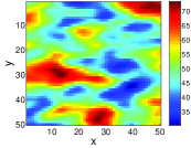
(a) Original data

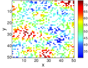
(b) Sample data

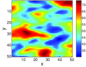
(c) Interpolated data

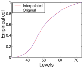
(d) Empirical cdf

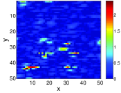
(e) 95% c.i. width

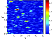
(f) RMSE

Figure 1: DGC interpolation results for synthetic Gaussian data with anisotropic Matérn covariance based on $M=100$ simulation runs on a single sample generated by $66\%$ thinning. Subfigures include (a) original field, (b) thinned sample, (c) interpolated data based on the median values from $M$ runs, (d) comparison of the empirical cdfs of the original and interpolated data, (e) spatial distribution of the $95\%$ confidence interval (c.i.) widths, and (f) root mean squared errors of predictions.

The classification results for the synthetic data are summarized in Table 1. The misclassification rate obtained by DGC is considerably smaller than the KNN and FKNN rates in all cases, although DGC shows somewhat larger sample-to-sample fluctuations. The mean CPU time required by DGC ranges between 0.96 and 1.11 seconds and the mean number of Monte Carlo steps between $10^{4}$ and $5\times 10^{4}$. The DGC interpolation performance is evaluated in Table 2 using $N_{c}=1000$ classes. In terms of validation errors (smallest errors and largest $R$), for the uniformly thinned data ($p=33\%,66\%$) OK ranked best. As mentioned above, for Gaussian data with known covariance parameters OK is expected to give optimal predictions. The known directional correlation lengths also allowed identifying a region of influence around the prediction points, thus optimizing search neighborhoods and consequently the OK CPU time. Nevertheless, the OK CPU time was the highest. For $p=33\%$ the DGC performance ranked second and for $p=66\%$ it was comparable to BS, with the other models performing worse than DGC. We note that DGC values in Tables 1 and 2 are based on $M=1$ simulation run for each of $S=100$ sample realizations. Increased values of $M$ (e.g. $M=100$) only marginally improved the validation results.

To account for more realistic patterns of missing data in remote sensing, e.g. due to cloud cover, we investigate a sample realization in which a solid block of data (rectangle of $16\times 8$ pixels) is missing (see Fig. 2). The block is deliberately chosen to include a small area with extreme values to test the ability of DGC to predict a “hotspot”. For this study, DCG performs better than the other methods. To compensate for using one sample $(S=1)$, we run $M=100$ simulations. Therefore the DGC CPU time is considerably higher compared to the (a) and (b) cases $(M=1)$.

The dramatic increase of the OK CPU time is caused by the augmented search neighborhood necessary to span the missing data gap and the cubic dependence of kriging on the number of points in the search neighborhood. Generally, the DGC CPU time is proportional to $N_{c}$ and increases with $p$, reflecting the increased dimension of the configuration space and number of variables involved in the optimization. For $p=66\%$ the optimization involves approximately $10^{6}$ Monte Carlo steps. As shown in Fig. 1, multiple simulation runs allow estimating the interpolation uncertainty, with respect to the subspace of configurations that correspond to local minima of the objective function (3).

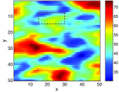
(a) OK interpolation

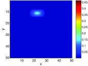
(b) OK variance

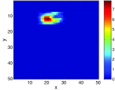
(c) OK absolute error

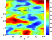
(d) DGC interpolation

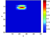
(e) DGC variance

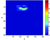
(f) DGC absolute error

Figure 2: Interpolation results for synthetic Gaussian data with anisotropic Matérn covariance. Sample data are generated by removal of a block of data in the area marked by the dashed rectangle. The DGC results are based on $M=100$ simulation runs. Subfigures show data interpolated by (a) OK and (d) DGC, variance by (b) OK and (e) DGC, and absolute errors by (c) OK and (f) DGC.

Table 2: Interpolation validation measures for Gaussian data with anisotropic Matérn covariance, using (a,b) $S=100$ samples generated by $33\%$ and $66\%$ random thinning, respectively, and (c) $S=1$ sample generated by removal of a solid block of data. The DGC uses $N_{c}=1000$ and the results are based on $M=1$ simulation run in (a) and (b) and $M=100$ simulation runs in (c).

	MAAE			MARE [%]			MAARE [%]			MRASE			$MR$ [%]			$\langle T_{cpu}\rangle$
	(a)	(b)	(c)	(a)	(b)	(c)	(a)	(b)	(c)	(a)	(b)	(c)	(a)	(b)	(c)	(a)	(b)	(c)
DGC	0.17	0.50	1.28	$-$0.01	$-$0.07	1.70	0.35	1.04	2.45	0.33	0.83	1.71	99.93	99.56	98.84	3.16	8.78	166
NN	2.08	2.09	5.01	$-$0.19	$-$0.17	8.12	4.25	4.26	9.77	2.65	2.73	6.24	95.61	95.35	75.52	0.04	0.02	0.08
BL	0.63	1.01	4.95	$-$0.12	$-$0.21	6.49	1.29	2.10	9.41	0.91	1.51	6.07	95.59	95.30	75.52	0.04	0.02	0.06
BC	0.43	0.78	4.92	$-$0.06	$-$0.12	6.82	0.89	1.61	9.32	0.65	1.21	6.09	99.74	99.09	79.00	0.04	0.02	0.06
BS	0.32	0.55	5.09	$-$0.02	$-$0.06	9.19	0.65	1.13	9.61	0.41	0.78	6.30	99.90	99.62	83.45	2.06	0.57	0.49
ID	1.04	1.44	5.14	$-$0.29	$-$0.33	7.33	2.15	2.96	9.85	1.34	1.91	6.22	99.09	97.84	77.06	0.16	0.17	0.06
OK	0.06	0.31	2.49	$-$1E-5	$-$0.01	4.66	0.12	0.65	4.71	0.12	0.49	3.19	99.99	99.85	96.75	31.1	9.15	2546

4.2 Real Data

4.2.1 Radioactive Potassium Concentration

The first real data set represents soil concentration of radioactive potassium measured by gamma-ray spectrometry over part of Canada (Anonymous,, 2008), on a grid with $N_{G}=256\times 256$ nodes extending in latitude from 56S to 57N and in longitude from $-$100W to $-$98E, with a resolution of 250 m. The data have been preprocessed to correct for background and airplane flight height. The potassium concentrations are in units of % and their summary statistics are as follows: $N_{G}=65536$, $z_{\min}=0.39$, $z_{\max}=3.26$, $\bar{z}=1.60$, $z_{0.50}=1.61$, $\sigma_{z}=0.52$, skewness coefficient equal to $0.10$, and kurtosis coefficient equal to $2.45$. A plot of the data in Fig. 3(a) displays clear signs of anisotropy. Samples ${\bf Z}(G_{s})$ were generated from the original data by random thinning with $p=33\%$ and $66\%$.

Classification $(N_{c}=8,16)$ and interpolation $(N_{c}=1500)$ results for $p=33\%$ are listed in Table 3. The prediction performance of DGC is superior to other models except for the BS. The outstanding performance of the latter is likely due to the smooth spatial variation of the radioactivity data. An example of prediction results based on $M=100$ simulation runs for one sample realization with $p=66\%$ is shown in Fig. 3. The DGC classification CPU time with $N_{c}=8,16$ was 2.6 and 3.3 seconds respectively. The computational time for DGC interpolation is comparable to that of BS, but one order higher than NN, BL, and BC times. The limiting factor in DGC are the MC simulations that involve up to $\sim 10^{7}$ Monte Carlo steps (see Fig. 4(a)). The histogram in Fig. 4(b) gives the distribution of the objective function residuals for 100 accepted configurations and verifies that all of them correspond to small $(<2\times 10^{-4})$ values.

(a) Original data

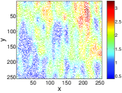
(b) Sample data

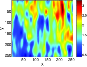
(c) Interpolated data

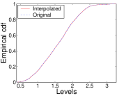
(d) Empirical cdf

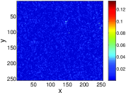
(e) 95% c.i. width

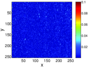
(f) RMSE

Figure 3: DGC interpolation of the radioactivity data obtained from $M=100$ simulation runs using one sample set generated by $66\%$ thinning. The plots are as those in Fig. 1.

Table 3: Classification ($N_{c}=8,16$) and interpolation $(N_{c}=1500)$ results for the radioactivity data with $p=33\%$ thinning. DGC is compared with k-nearest neighbor (KNN) and fuzzy k-nearest neighbor (FKNN) models for classifications, and with the nearest neighbor (NN), bilinear (BL), bicubic (BC), biharmonic spline (BS) and inverse distance (ID) models for interpolation.

	Classification				Interpolation
	$N_{c}=8$		$N_{c}=16$		$N_{c}=1500$
Model	$\langle F^{*}\rangle$	${\rm S}_{F^{*}}$	$\langle F^{*}\rangle$	${\rm S}_{F^{*}}$	MAAE	MARE [%]	MAARE [%]	MRASE	$MR$ [%]	$\langle T_{cpu}\rangle$
DGC	4.01	0.21	8.64	0.28	9.4e$-$4	$-$2.2e$-$3	6.8e$-$2	1.56e$-$3	100.00	39.94
KNN	4.96	0.16	11.44	0.22	-	-	-	-	-	-
FKNN	4.22	0.16	10.14	0.23	-	-		-	-	-
NN	-	-	-	-	2.3e$-$2	-0.165	1.64	3.5e$-$2	99.78	1.41
BL	-	-	-	-	3.7e$-$3	-5.9e$-$2	0.27	5.9e$-$3	99.78	1.40
BC	-	-	-	-	1.7e$-$3	-2.2e$-$2	0.12	2.9e$-$3	100.00	1.46
BS	-	-	-	-	4.7e$-$4	-1.2e$-$3	3.4e$-$2	7.6e$-$4	100.00	32.82
ID	-	-	-	-	1.3e$-$2	-0.160	0.90	1.7e$-$2	99.95	183.64

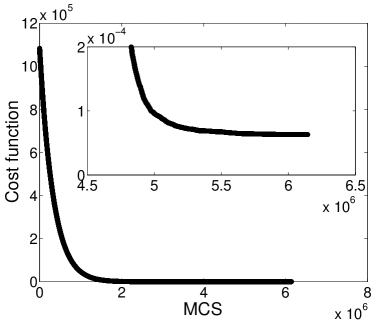
(a) Objective function evolution

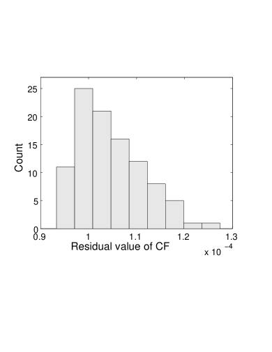
(b) Residual objective function

Figure 4: Left: Evolution of the objective (cost) function (3) for potassium concentration versus the number of Monte Carlo steps. Inset focuses on the convergence to the optimum. Right: Histogram of the objective function residual values obtained from $100$ different runs.

4.2.2 Ozone Layer Thickness

The second real-world data set represents daily column ozone measurements on June 1, 2007 (Acker and Leptoukh,, 2007). The data are on a $1^{\circ}\times 1^{\circ}$ grid with $N_{G}=180\times 360$ nodes extending in latitude from 90S to 90N and in longitude from 180W to 180E. The data set includes naturally missing (and therefore unknown) values. The data are in Dobson units with the following summary statistics: $N=48501$, $z_{\min}=158$, $z_{\max}=596$, $\bar{z}=311.58$, $z_{0.50}=308$, $\sigma_{z}=46.05$, skewness coefficient equal to $0.31$, and kurtosis coefficient equal to $2.30$. The gaps are mainly due to limited coverage on the particular day, generating conspicuous stripes of missing values in the south-north direction. Since the true values at these locations are not known, validation measures are not evaluated. Instead, the interpolation quality is assessed empirically, based on the visual continuity between the observed data and the predictions.

In the DGC reconstructed image, as shown in Fig. 5(b), some traces of the stripe pattern due to overestimation in low-value areas (averaging effect) can still be observed. However, this effect is somewhat less pronounced than in other interpolation methods, presented in Fig. 6. Indeed, histograms of the predicted values, see Fig. 7, show a larger proportion of DGC predictions in bins below the sample average $\bar{z}=311.58$ compared to the other methods.

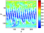
(a) Gappy ozone data

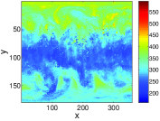
(b) DGC interpolation

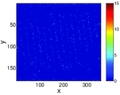
(c) 95% c.i. width

Figure 5: DGC interpolation results for ozone data, obtained from $M=100$ simulation runs on one set of the original data with missing values: Original data (a), interpolated data based on the median values from $M$ runs (b), and spatial distribution of the $95\%$ confidence interval (c.i.) widths (c).

(a) NN interpolation

(b) ID interpolation

(c) BS interpolation

Figure 6: Interpolation results for ozone data, using the nearest-neighbor (NN) (a), the inverse distance (ID) (b), and the biharmonic spline (BS) (c) methods.

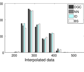
Figure 7: Histograms of the ozone values predicted by the respective methods: DGC, NN, ID, and BS.

5 Discussion and Conclusions

We presented and investigated the DGC method for the prediction of missing data on rectangular grids. DGC is based on stochastic simulation conditioned by sample data with a global objective function that accounts for anisotropic correlations. The constraints involve normalized directional gradient and curvature energies in specified directions. The simulation samples the configuration subspace that leads to local minima of the objective function.

For reliable application of DGC sufficiently high sampling density and number of data for the calculation of sample constraints are desirable. We evaluated the average numbers $n_{p}$ of nearest-neighbor sampling-point pairs per direction and $n_{t}$ of compact triplets of sampling points per direction. The first, $n_{p}$, is equal to the number of terms involved in $\overline{G}_{n}({\bf I}_{s})$, while the second, $n_{t}$, is the number of terms in $\overline{C}_{n}({\bf I}_{s})$. For uniform random thinning $n_{p}$ and $n_{t}$ depend only on the degree of thinning $p$ and the domain size $L$. For $p=66\%$ we obtained $(n_{p},n_{t})=(280,92)$ for $L=50$ and $(n_{p},n_{t})=(7523,2542)$ for $L=256$ without significant differences between different directions. These values are sufficient for reliable estimates of $\overline{G}_{n}({\bf I}_{s})$ and $\overline{C}_{n}({\bf I}_{s})$. However, smaller grids or higher thinning degrees can lead to insufficient sampling.

Regarding sensitivity of DGC to noise, we have run tests on simulated random field realizations to which Gaussian white noise is added. DGC seems more sensitive to noise than other interpolation methods (e.g., BL, BC, BS), resulting in a larger increase of cross-validation errors with increasing noise variance. This effect is caused by the fact that methods like BL, BC, and BS perform some smoothing of the noise by means of the weighted average over extended neighbors. DGC on the other hand focuses on correlations over a small local neighborhood, which are sensitive to noise. Hence, in its current formulation DGC is more useful for smooth data distributions, such as the ones studied herein. For noisy data, improvements can be made by developing directional kernel-based estimators for the square gradient and curvature in the spirit of (Elogne & Hristopulos,, 2008; Hristopulos & Elogne,, 2009) or by incorporating an initial filtering stage to reduce noise (Brownrigg,, 1984; Yin,, 1996).

DGC does not rely on assumptions about the probability distribution of the data, it is reasonably efficient computationally, and it requires very little user input (i.e., the number of simulation runs, the number of class levels and the size of the maximum stencil for initial state selection). Potential applications include filling of data gaps in satellite images and restoration of damaged digital records. For applications in the interpolation of data sampled on an irregular grid, DGC needs to be extended to account for the lack of grid structure. This can be accomplished using kernel functions with adjustable bandwidth as shown in (Elogne & Hristopulos,, 2008; Hristopulos & Elogne,, 2009).

DGC shares conceptual similarities with interpolation methods based on splines, which are generated by minimizing an objective function formed by the linear combination of the square gradient and the square curvature (Wessel,, 2009). A special case of the splines-based approach is the BS method used above for comparison purposes. DGC does not require minimization of the square gradient and curvature but requires matching the sample and entire-grid values of these constraints. Splines-based methods require solving a linear system involving the Green’s function of the interpolation operator; the numerical complexity of this calculation scales with the third power of the system size. DGC does not require such a costly operation, because the objective functional is defined using local couplings. Finally, in contrast with splines interpolation, DGC introduces a stochastic element by sampling the configuration subspace of local minima of the DGC objective function. On the other hand, splines-based methods can handle irregularly spaced samples, while DGC is currently restricted to grid data.

References

References

- Acker and Leptoukh, (2007) Acker, J.G., Leptoukh, G., 2007. Online Analysis Enhances of NASA Earth Science Data , Eos, Trans. AGU, Vol. 88, No. 2 (9 January 2007), 14-17. Online at: http://disc.sci.gsfc.nasa.gov/giovanni/
- Akbas, (2007) Akbas, E., 2007. Fuzzy k-NN (http://www.mathworks.com/matlabcentral/fileexchange/13358-fuzzy-k-nn), MATLAB Central File Exchange. Retrieved August 10, 2008.
- Albert et al., (2012) Albert, M.F.M.A., Schaap, M., Manders, A.M.M., Scannell, C. , O’Dowd, C.D. , de Leeuw, G., 2012. Uncertainties in the determination of global sub-micron marine organic matter emissions. Atmospheric Environment, 57(9), 289-300.
- Anonymous, (2008) Anonymous, 2008. National Gamma-Ray Spectrometry Data Base, Geoscience Data Repository, Geological Survey of Canada, Earth Sciences Sector, Natural Resources Canada, Government of Canada. Online at: http://www.nrcan.gc.ca/earth-sciences/home
- Bechle et al., (2013) Bechle, M.J., Millet, D.B., Marshall, J.D. Remote sensing of exposure to NO2: satellite versus ground based measurement in a large urban area. Atmospheric Environment, Available online 13 December 2012, doi: 10.1016/j.atmosenv.2012.11.046.
- Brownrigg, (1984) Brownrigg, D.R.K., 1984. The weighted median filter. ACM Communications, 27(8), 807-818.
- Cressie, (2008) Cressie, N., 2008. Fixed rank kriging for very large spatial data sets. Journal of the Royal Statistical Society Series B, 70(1), 209-226.
- Dasarathy, (1991) Dasarathy, B.V. (Ed.), 1991. Nearest neighbor norms: NN pattern classification techniques. IEEE Computer Society Press, Los Alamitos, CA.
- Diggle & Ribeiro, (2007) Diggle, P.J., Ribeiro, Jr., P.J., 2007. Model-based Geostatistics. Series: Springer series in statistics. Springer, New York.
- Drummond and Horgan, (1987) Drummond, I.T., Horgan, R.R., 1987. The effective permeability of a random medium. Journal of Physics A, 20, 4661-4672.
- Elogne & Hristopulos, (2008) Elogne S.N., Hristopulos D.T., 2008. Geostatistical applications of Spartan spatial random fields. In: Proceedings of the 6th International Conference on Geostatistics for Environmental Applications, Rhodes, Greece: October 2006. Eds. A. Soares and M.J. Pereira and R. Dimitrakopoulos, Vol. 15, pp. 477-488, Springer, Berlin.
- Emili et al., (2011) Emili, E., Popp, C., Wunderle, S., Zebisch, M., Petitta, M., 2011. Mapping particulate matter in alpine regions with satellite and ground-based measurements: An exploratory study for data assimilation. Atmospheric Environment, 45(26), 4344-4353.
- Hartman & Hössjer, (2008) Hartman, L., Hössjer, O., 2008. Fast kriging of large data sets with Gaussian Markov random fields. Computational Statistics and Data Analysis, 52, 2331 - 2349.
- Howat, (2007) Howat, I.M., 2007. Filling NaNs in array using inverse-distance weighting. (http://www.mathworks.com/matlabcentral/fileexchange/15590-fillnans), MATLAB Central File Exchange. Retrieved June 15, 2009.
- Hristopulos, (2003) Hristopulos, D.T., 2003. Spartan Gibbs random field models for geostatistical applications, SIAM Journal in Scientific Computation, 24, 2125-2162.
- Hristopulos & Elogne, (2009) Hristopulos, D.T., Elogne, S.N., 2009. Computationally efficient spatial interpolators based on Spartan spatial random fields, SIAM Journal in Scientific Computation, 57(9), 3475-3487.
- Jun & Stein, (2004) Jun, M., Stein, M.L., 2004. Statistical comparison of observed and CMAQ modeled daily sulfate levels. Atmospheric Environment, 38(27), 4427-4436.
- Junninen et al., (2004) Junninen, H., Niska, H., Tuppurainen, K., Ruuskanen, J., Kolehmainen, M., 2004. Methods for imputation of missing values in air quality data sets. Atmospheric Environment, 38(18), 2895-2907.
- Keller et al., (1985) Keller, J.M., Gray, M.R., Givens, J.A.Jr., 1985. Fuzzy k-nearest neighbor algorithm. IEEE Transactions on Systems, Man and Cybernetics, 15, 580-585.
- Lehman et al., (2004) Lehman, J., Swinton, K., Bortnick, S., Hamilton, C., Baldridge, E., Eder, B., Cox, B. 2004. Spatio-temporal characterization of tropospheric ozone across the eastern United States. Atmospheric Environment, 38(26), 4357-4369.
- Papadimitriou & Steiglitz, (1982) Papadimitriou, C.H., Steiglitz, K., 1982. Combinatorial Optimization. Prentice Hall, New Jersey.
- Sandwell, (1987) Sandwell, D.T., 1987. Biharmonic Spline Interpolation of GEOS-3 and SEASAT Altimeter Data. Geophysical Research Letters, 14, 139-142.
- Shepard, (1968) Shepard, D., 1968. A two-dimensional interpolation function for irregularly-spaced data. Proceedings of the 1968 ACM National Conference, 517-524.
- Sickles & Shadwick, (2007) Sickles, J.E., Shadwick, D.S., 2007. Effects of missing seasonal data on estimates of period means of dry and wet deposition. Atmospheric Environment, 41(23), 4931-4939.
- Sidler, (2009) Sidler, R., 2009. vebyk: Value Estimation BY Kriging. (http://www.mathworks.com/matlabcentral/fileexchange/4566-vebyk), MATLAB Central File Exchange. Retrieved June 15, 2009.
- Wackernagel, (2003) Wackernagel, H., 2003. Multivariate Geostatistics. Springer, New York.
- Wessel, (2009) Wessel, P., 2009. A general-purpose Green’s function-based interpolator. Computers & Geosciences, 35(6), 1247-1254.
- Yin, (1996) Yin, L., Yang, R.K., Gabbouj, M., Neuvo, Y., 1996. Weighted median filters: A tutorial. IEEE Transactions on Circuits and Systems II, 43(3), 157 192.
- Žukovič & Hristopulos, (2012) Žukovič, M., Hristopulos D.T., 2012. Reconstruction of missing data in remote sensing images using conditional stochastic optimization with global geometric constraints, Stoch Environ Res Risk Assess, Available online 4 Spetember 2012, doi: 10.1007/s00477-012-0618-5.