Reverse dynamical evolution of Eta Chamaeleontis

Abstract

Context. In the scope of the star formation process, it is unclear how the environment shapes the initial mass function (IMF). While observations of open clusters propose a universal picture for the IMF from the substellar domain up to a few solar masses, the young association $\eta$ Chamaeleontis presents an apparent lack of low mass objects ($m<0.1\$$\text{M}_{\odot}$). Another unusual feature of this cluster is the absence of wide binaries with a separation $>50$ AU.

Aims. We aim to test whether dynamical evolution alone can reproduce the peculiar properties of the association under the assumption of a universal IMF.

Methods. We use a pure N-body code to simulate the dynamical evolution of the cluster for 10 Myr, and compare the results with observations. A wide range of values for the initial parameters are tested (number of systems, typical radius of the density distribution and virial ratio) in order to identify the initial state that would most likely lead to observations. In this context we also investigate the influence of the initial binary population on the dynamics and the possibility of having a discontinuous single IMF near the transition to the brown dwarf regime. We consider as an extreme case an IMF with no low mass systems ($m<0.1\$$\text{M}_{\odot}$).

Results. The initial configurations cover a wide range of initial density, from $10^{2}$ to $10^{8}$ stars/$\text{pc}^{3}$, in virialized, hot and cold dynamical state. We do not find any initial state that would evolve from a universal single IMF to fit the observations. Only when starting with a truncated IMF without any very low mass systems and no wide binaries, can we reproduce the cluster core properties with a success rate of 10% at best.

Conclusions. Pure dynamical evolution alone cannot explain the observed properties of $\eta$ Chamaeleontis from universal initial conditions. The lack of brown dwarfs and very low mass stars, and the peculiar binary properties (low binary fraction and lack of wide binaries), are probably the result of the star formation process in this association.

1 Introduction

As an imprint of the star formation process and governing the evolution of star populations, the initial mass function (IMF) has been studied in depth in the solar neighbourhood as well as in young open clusters. Particular interest has been devoted to the question of the universality of the IMF: is there a unique mass distribution resulting from the interplay of physical processes of star formation, or does it vary with gas density, metallicity (Marks et al. 2012) or turbulence?
Introduced by Salpeter (1955), the IMF was first described for stars in the mass range $0.4$ $\text{M}_{\odot}$ to $10$ $\text{M}_{\odot}$ as a power law $\xi(\log\ m)=\frac{dn}{d\log\ m}\propto m^{-\Gamma}$, with $\Gamma=1.35$ in logarithmic scale. This field star power-law index was independently established by Kroupa et al. (1993a) for $0.5$ $\text{M}_{\odot}$ to $1$ $\text{M}_{\odot}$ and extended by Massey (2003) to $10$ $\text{M}_{\odot}$. Focussing on close open clusters, e.g. the Pleiades (Moraux et al. 2003; Lodieu et al. 2007), IC 4665 (de Wit et al. 2006), $\alpha$ Per (Barrado y Navascués et al. 2002), or Blanco 1 (Moraux et al. 2007a), it was possible to explore the system (i.e. incorporating both single objects and unresolved binaries) mass function in the lower mass regime down to $\simeq$ 0.03 $\text{M}_{\odot}$. Investigations on the shape of the mass function in various environments show some deviations that can be explained by uncertainties due to e.g. different sampling, dynamical evolution, and stellar evolution models, but show no evidence for any significant variation (Scalo 2005; Bastian et al. 2010).These studies lead to a universal picture of the system IMF down to 0.03 $\text{M}_{\odot}$(see review of Kroupa et al. 2011) as a non-monotonic function showing a maximum around 0.25 $\text{M}_{\odot}$ and a power-law tail at the high mass end. Many functional forms can be tailored to this IMF, e.g. segmented power-laws (Kroupa et al. 1993b), a log-normal function plus a power-law tail (Chabrier 2003), or a tapered power law (de Marchi et al. 2005; Parravano et al. 2011; Maschberger 2012).
In this paper, the universality of the IMF is investigated by focussing on the dynamical evolution of the stellar group $\eta$ Chamaeleontis. Since its discovery by Mamajek et al. (1999) this cluster has been the target of many observational studies (e.g Luhman 2004; Brandeker et al. 2006; Lyo et al. 2003). It is a young (6-9 Myr, Lawson & Feigelson 2001; Jilinski et al. 2005), close (d $\simeq$ 94 pc) and compact group of 18 systems (contained in a radius of 0.5 pc). Its system mass function was found to be consistent with that of other young open clusters and the field (Lyo et al. 2004) in the mass range 0.15-3.8 $\text{M}_{\odot}$, but with a lack of lower mass members. This challenges the universal picture of the IMF, unless the observed present day mass function has already been affected by dynamical evolution. Despite deep and wide-field surveys (Luhman 2004; Song et al. 2004; Lyo et al. 2006), no very low mass systems ($m\lesssim 0.1$ $\text{M}_{\odot}$) was found within 2.6 pc from the center. A recent study by Murphy et al. (2010) reported the discovery of four probable and three possible low mass members ($m<0.3$ $\text{M}_{\odot}$) in the outer region, between 2.6 and 10 pc from the cluster center. This suggests that the lower mass members might have escaped from the cluster core due to dynamical encounters and lie at larger radii than the more massive members. Moreover, the cluster appears to be mass segregated with all the massive stars ($m>1.5$ $\text{M}_{\odot}$) concentrated in its very central region, which supports the picture of dynamical evolution. Among the 18 systems 5 are confirmed binaries and 3 are possible binaries yielding a binary fraction in the range [28%,44%]. As summarised by Brandeker et al. (2006), none of these binaries have a projected separation greater than 20 AU, and the probability for a star to have a companion at separations larger than 30 AU was estimated to be less than 18%. This is opposed to the 58% wide binary probability in the TW Hydrae association (Brandeker et al. 2003), despite its similar age. This deficit of wide binaries in $\eta$ Chamaeleontis may also be explained by their disruption through dynamical interactions.
In a previous study (Moraux et al. 2007b), we considered whether dynamical interactions could explain the lack of very low mass systems ($m<0.1$ $\text{M}_{\odot}$) in the cluster core, starting with a universal IMF. We applied an inverse time integration method by sweeping the parameter space for the initial state in order to find those that best lead, as a result of a pure N-body simulation, to the observed properties of $\eta$ Cha. This method has been applied in numerous earlier studies (e.g Kroupa 1995a; Kroupa & Bouvier 2003; Marks & Kroupa 2012) to obtain a comprehensive picture of the early dynamical evolution of star clusters. In our case this was designed as a test of the universality of the IMF. Assuming a log-normal shape for the system IMF (Chabrier 2003) we span a large range of initial densities. We found that it was possible to reproduce the observations starting from a very dense configuration ($10^{8}$ stars/$\text{pc}^{3}$) with a success rate of 5%. The simulations, however, did not include any primordial binaries nor considered the creation of binaries in the detailed analysis. The gas was removed initially and we assumed that the cluster was in virial equilibrium.
In the present study, we follow the same method in an attempt to reproduce the observed state of $\eta$ Cha, but we now take into account an initial binary population and its evolution. In a first set of models, we assume a universal log-normal IMF (Chabrier 2005) before considering a possible discontinuity (Thies & Kroupa 2007) around the substellar limit, and a truncated IMF with no system below 0.1 $\text{M}_{\odot}$. The simulations still start after the gas has been expelled but virial equilibrium is not required.
The outline of this paper is as follows: we first discuss the statistical significance of the deficit of very low mass systems ($m<0.1$ $\text{M}_{\odot}$) in the cluster core (Section 2) before describing the numerical scheme adopted for the simulations, especially the initial conditions and the parameter grid (Section 3). The analysis procedure is introduced in Section 4. Section 5 presents the results obtained when starting with a log-normal IMF. We discuss alternative initial conditions in Section 6 before presenting our conclusions.

2 Statistical issues

With less than 20 systems in the cluster core, the statistical analysis of $\eta$ Cha has to be done carefully, especially when considering a standard distribution such as the IMF. In the range from 0.15 to 4 $\text{M}_{\odot}$, the $\eta$ Cha mass function (MF) was found to be consistent with the IMF derived for young embedded clusters (Lyo et al. 2004; Meyer et al. 2000) and field stars by comparing the ratio of stars with mass $m>1\ \text{M}_{\odot}$ to stars with mass $0.1<m<1\leavevmode\nobreak\ \text{M}_{\odot}$. Lyo et al. (2004) predicted about 20 members with $m<0.15\ \text{M}_{\odot}$ by comparison with the Trapezium MF. None has been found within a 2.6 pc radius despite deep and wide searches, indicating a strong deficit of very low mass systems in $\eta$ Cha. However, using a Kolmogorov-Smirnov (KS) test, Luhman et al. (2009) derived a probability of $\simeq$10% that $\eta$ Cha is drawn from the same IMF as Chameleon I or IC348, not revealing significant differences between those distributions. One can therefore wonder whether the lack of very low mass objects (single stars/brown dwarfs or unresolved binaries with $m<0.1\ \text{M}_{\odot}$, hereafter VLMOs) inside a 2.6 pc radius from the cluster center represents a significant deviation from the universal MF of open clusters.

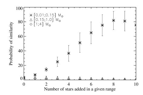
Figure 1: KS test evaluating the similarity of the $\eta$ Cha mass distribution with the log-normal system IMF. The comparison is done considering three mass ranges, in order to assess which parts of the distribution are alike. We progressively added ten stars in $\eta$ Cha data set, selected randomly from the IMF within the mass range [0.01;0.15] $\text{M}_{\odot}$. Each time a star is added we compute a probability from the KS test. This process is repeated for the mass ranges [0.15;1] $\text{M}_{\odot}$ and [1;4] $\text{M}_{\odot}$.

If we choose the log-normal fit to the Pleiades system MF as a reference (Moraux et al. 2003), then the KS probability for testing the hypothesis that the stellar masses in $\eta$ Cha are chosen from this log-normal MF is 2.8 %. To assess the sensitivity of this result to the data set, we present in Fig. 1 the evolution of the KS probability while systems are randomly added to the list of known $\eta$ Cha members from three different mass ranges ([1-4] $\text{M}_{\odot}$, [0.15-1] $\text{M}_{\odot}$ and [0.01-0.15] $\text{M}_{\odot}$). The probability increases uniformly to 80% until eight systems with $m<0.15$ $\text{M}_{\odot}$ are added, which points out the importance of the deficit of VLMOs relatively to medium and high mass stars. However the KS probability is already greater than 5% when only one such system is added, and we cannot reject the possibility that this data set is drawn from the MF used as reference. As a result, a paucity of VLMOs may be present but it might not be statistically inconsistent with the Pleiades MF.
Nevertheless, even if the deficit of very low mass systems is not really significant, it is additional to the other peculiar properties that also need to be understood: the lack of wide binaries with separation larger than 20 AU, and the presence of mass segregation.

3 Numerical set-up

In this Section we describe the physical properties that we tested in our models: the single initial mass function (of all stars counted individually) and the primordial binary properties (binary fraction, separation and mass ratio distribution). We then review the assumptions corresponding to the lack of gas treatment and the density profile, and we present the parameter grid that we used for each model: the number of systems, the characteristic spatial scale for the density distribution function, and the global virial ratio.

3.1 IMF

As our main hypothesis we choose a single IMF of log-normal form as suggested by Miller & Scalo (1979)

$$\xi\text{(}log\ m)\ \propto\ \exp\left[-\frac{(\text{log}\ m\ -\text{log}\ \mu)^{2}}{2\sigma^{2}}\right]$$

This function was fitted in the 0.1-1 $\text{M}_{\odot}$ mass range to the nearby galactic disk MF based on a volume limited sample within 8 pc and yields $\mu=$ 0.2 $\text{M}_{\odot}$ and $\sigma=$ 0.55 (Chabrier 2005). A similar result was obtained by Bochanski et al. (2010) for the field M-dwarf MF based on a much larger (several million stars), but unresolved sample. In order to test its universality, we use the single IMF proposed by Chabrier (2005) in our models A, B and C. Masses were chosen within a mass range consistent with observation, from 0.01 to 4 $\text{M}_{\odot}$.
As an alternative, we test the possibility that the single star IMF may be discontinuous (model D) with the majority of brown dwarfs following their own IMF, as suggested by Thies & Kroupa (2007). Since this may result in a lower number of VLMOs in the cluster initially, we might expect this initial condition to be more favourable in reproducing the observations.
We also study the extreme case where the IMF is not universal but truncated in the low mass domain, with no system below 0.1 $\text{M}_{\odot}$ to follow the observations (models E and F).

3.2 Binary properties

Observations of young clusters reveal a broad range of binary fractions $b_{f}$, defined as $\displaystyle b_{f}\ =\ \frac{N_{b}}{N_{b}+N_{s}}$, where $N_{b}$ is the number of binaries and $N_{s}$ the number of single objects. According to N-body numerical simulations (Kroupa 1995a), this is consistent with a universal initial binary fraction of 100% that decreases with time depending on the star cluster density. We thus fixed the initial binary fraction to $b_{f}=$100% for most of our models (except model C and F).
Concerning the mass-ratio distribution, we draw two masses randomly (in Model A) from the same single IMF in order to get the primary and the secondary masses ; the approach adopted by Kroupa (1995a). For all other models (except Model D) we adopted a flat mass-ratio distribution (Reggiani & Meyer 2011), and the IMF used to obtain the mass for the primary had to adjusted (see section 6.1) so that once the pairing is done we retrieve the single IMF from Chabrier (2005) presented above.
As for the separation distribution, we took the one derived by Kroupa et al. (2011) (see their equation 46) to fit the observational data for F, G and K field stars (Duquennoy & Mayor 1991; Raghavan et al. 2010) using inverse dynamical population synthesis and taking into account early evolution of the orbital parameters for small period systems. The separation distribution ranges from 0.1 AU to $10^{5}$ AU for the models A, B, D and E. In accordance with conclusions of the work by Kroupa et al. (2011), we also chose an initial eccentricity distribution already in statistical equilibrium to ensure a thermal final distribution. Although observations of multiple systems rather support an essentially flat distribution of eccentricity (e.g Abt 2006), we note that dynamical simulations are hardly sensitive to the selected eccentricity distribution (Kroupa 1995b). We therefore favour consistency with previous work to enable direct comparisons.
Given the observed lack of wide binaries, we consider the possibility that no wide binary has formed initially. Instead of assuming a Kroupa-like separation distribution we also explore a truncated distribution at large separation together with a smaller binary fraction (models C and F, see section 6.2).
A summary of all considered models is given in Table 1.

Table 1: Physical properties corresponding to each model.

	log-normal IMF	discont. IMF	truncated IMF
$b_{f}=$100% + random pairing	model A	model D
$b_{f}=$100% + flat mass ratio	model B		model E
separation cut-off + flat mass ratio	model C		model F

3.3 Gas

For all our models, we assume that the gas is already removed at the start of the simulations, but that the cluster is not necessarily relaxed to virial equilibrium. We estimate that our initial state depicts a cluster that is between 0.1 Myr to 3 Myr old, depending on the picture for gas removal (Tutukov 1978). Indeed, there is no clear consensus about the time scale for gas dispersal, estimated from 0.1 to a few crossing times, depending on the mechanism in play (OB star wind, supernovae remnant or stellar outflows). In the case of $\eta$ Cha, the mechanism for gas removal may involve an external factor on a time scale that could be as long as a few Myr. Ortega et al. (2009) proposed a common formation scenario for young clusters in the Scorpio-Centaurus OB association ($\eta$ Cha, $\epsilon$ Cha and Upper Sco), by backtracking bulk motions. In this dynamical picture, $\eta$ Cha was born in a medium likely being progressively blown out by strong stellar winds coming out from the Lower and Upper Centaurus Crux complex. Another possibility to expel the gas from the cluster may involve feedback from a massive stellar member. Moraux et al. (2007b) showed that $\eta$ Cha initial state might have been very compact, with a crossing time of about $2\leavevmode\nobreak\ 10^{4}$ yrs (for a total mass of 15 $\text{M}_{\odot}$ and a radius of 0.005 pc). In this extreme case, the presence of one B8 star (after which the cluster is named) might be sufficient to remove the gas within $10^{5}$ years. With a cluster age estimate of $8\pm 1$ Myr, we run the simulations for 10 Myr.

3.4 Density and velocity distribution

For all models, the systems are distributed spatially using a Plummer model

$$\rho_{\text{Pl}}(r)=\frac{3N_{\text{sys}}}{4\pi R_{\text{Pl}}^{3}}\left[1+(r/R_{\text{Pl}})^{2}\right]^{-5/2}$$

where $N_{\text{sys}}$ is the initial number of systems.
The velocities of each individual object are computed according to this density distribution and to the initial virial ratio $Q_{i}\ =\ {E_{kin}}/{E_{pot}}$ where $E_{kin}$ is the total kinetic energy of the cluster and $E_{pot}$ the gravitational energy. For each model, we are thus left with three free parameters: the initial number of systems $N_{\text{sys}}$, the Plummer radius $R_{\text{Pl}}$ and the virial ratio, $Q_{i}$.

3.5 Parameter grid

Table 2: Parameter grid for model A. We considered all combinations of $N_{\text{sys}}$, $R_{\text{Pl}}$, and $Q_{i}$

$N_{\text{sys}}$	20	30	40	50	60	70
$R_{\text{Pl}}$ (pc)	0.3	0.1	0.05	0.03	0.01	0.005
$Q_{i}$	0.3	0.4	0.5	0.6	0.7

From the shape of the IMF, we estimated an initial value of $N_{\text{sys}}=50$ by the requirement to have four stars with mass greater than 1 $\text{M}_{\odot}$. To cover a wide range of densities at fixed radius, we tested $N_{\text{sys}}$ from 20 to 70. The initial cluster radius was first estimated to fit a constant surface density derived from observations of star forming regions (Adams et al. 2006), giving 0.3 to 1.0 pc for 50 systems. The study of Moraux et al. (2007b) showed that a dense initial configuration was necessary in order to eject enough members from the cluster core and reproduce the lack of VLMOs. To favour dynamical interactions, we took a radius varying from 0.3 to 0.005 pc, yielding a density range from 500 stars/$\text{pc}^{3}$ to $10^{8}$ stars/$\text{pc}^{3}$. In order to assess the effect of initial equilibrium, we tested cold, gravitation-dominated configuration ($Q_{i}\ =\ 0.3$) and hot, initially expanding configuration ($Q_{i}\ =\ 0.7$).
For each model (A to F), an initial configuration is characterized by a combination of {$N_{\text{sys}}$, $R_{\text{Pl}}$, $Q_{i}$} from the values given in Table 2. In total, 180 arrangements were tested for each model.

3.6 N-body code

We use the NBODY3 code (Aarseth 1999) that performs a direct force summation to compute the dynamical evolution of the cluster. Close encounters are treated by Kustaanheimo-Stiefel (KS) regularization for hard binaries (Kustaanheimo & Stiefel 1965), which uses a space-time transformation to remove the singularity and then simplify the two body treatment, or chain regularization method (Mikkola & Aarseth 1990) for few body interactions (e.g. binary-single star). There is no stellar evolution.

3.7 Modelling procedure

The time evolution of the initial conditions described earlier produces output of positions and velocities for each star every 0.05 Myr. The NBODY3 output files also provide details for close binaries (semi-major axis, eccentricity) identified as bound double systems.The stellar cluster is put in a galactic potential that defines its tidal radius:

$$r_{t}=\left(\frac{G\ M}{4A(A-B)}\right)^{1/3}\simeq 1.4\ M^{1/3}\ \textrm{pc}$$

where $M$ is the cluster total mass (in solar masses) and $A$ and $B$ are the Oort constants (King 1962). Given the parameter grid, the initial $r_{t}$ value varies between 3.1 and 4.8 pc (the estimated value for $\eta$ Cha is around 3.5 pc assuming a total mass of 15 $\text{M}_{\odot}$, Lyo et al. (2004)). Objects are considered as being ejected and then removed from the simulation as soon as they are further than twice the cluster tidal radius from the center.
For each initial configuration {$N_{\text{sys}}$, $R_{\text{Pl}}$, $Q_{i}$} we generated 200 simulations, changing only the random seed, for statistical purposes. Every simulation computed the cluster dynamical evolution for 10 Myr.

4 Analysis procedure

In order to retrieve as much information as possible we analyse our set of simulations in two different ways for each model. First we consider the same analysis procedure as in Moraux et al. (2007b) that aims at finding final states that fit the observational data. Secondly, in order to better understand the results of the first analysis, we perform a statistical analysis. Both methods are based upon a set of constraints derived from the observations.

4.1 Observational criteria

We use a set of criteria described below to evaluate if a simulation at a given time is close to reproducing the observations. Each criterion is associated with a range of validity assuming Poisson statistics: a criterion $i$ is satisfied if $N_{i}\in[O_{i}-\sqrt{O_{i}},O_{i}+\sqrt{O_{i}}]$, where $N_{i}$ is obtained by simulation and $O_{i}$ is given by the observations. A summary of the chosen ranges is given in Table 3.

Table 3: Selection range adopted for the observational criteria

Criterion	Range	Restricted to
Systems	$N_{1}=[14,22]$	$r<0.5$ pc
Massive stars	$N_{2}=[2,4]$	$r<0.5$ pc
		$m>1.5$ $\text{M}_{\odot}$
VLMOs	$N_{3}=[0,1]$	$r<2.6$ pc
		$m<0.1$ $\text{M}_{\odot}$
Halo	$N_{4}=[0,1]$	$0.5<r<10$ pc
		$m>0.5$ $\text{M}_{\odot}$
Binary fraction	$N_{5}=[22,50]$%	$r<0.5$ pc
Wide binaries	$N_{6}=[0,1]$	$[50;400]$ AU
		$r<0.5$ pc
Time	[5,8] Myr	-

Number of systems ($N_{1}$)

To account for the membership and compactness of the core, we consider the total number of systems in a $0.5$ pc sphere. Since 18 systems have been observed within the core radius, we choose the range of 14 to 22 systems for a simulation to fulfil this criterion. Unless mentioned otherwise the term system refers to a single object or a binary of any mass within the stellar or substellar domain.
To take into account observational limitations in the comparison between simulations and observations, we identify binaries as closest neighbour pairs in projection (i.e. not necessarily bound) with a separation smaller than 400 AU (which corresponds to 4” at the cluster’s distance). At larger separations binaries are observationally identified as two single objects (Köhler & Petr-Gotzens 2002).

Number of massive stars ($N_{2}$)

Since three systems were found in the central region with a mass $m>1.5$ $\text{M}_{\odot}$, we require to have between $2$ and $4$ of them in the simulations. When counting massive stars, a binary system is considered as a single object with a mass corresponding to its total mass.

Number of systems in the halo ($N_{3}$)

No potential cluster member has been identified by the ROSAT All Sky Survey (sensitive to late-K type stars) outside the cluster core up to a distance of 10 pc. This translates into the following criterion: less than one cluster member more massive than 0.5 $\text{M}_{\odot}$ must lie within the distance range [0.5-10] pc from the cluster center.
Recently Murphy et al. (2010) have discovered four probable and three possible less massive members (in the spectral range K7 to M4, i.e. $0.1\text{M}_{\odot}\leavevmode\nobreak\ <m<0.3$ $\text{M}_{\odot}$) at a distance between 2.6 pc and 10 pc from the cluster centre. However, since the status of these candidates is not confirmed, we will check a posteriori that some simulations matching all other criteria do produce a number of low-mass halo stars that is consistent with the small number suggested by Murphy’s study.

Number of very low mass objects ($N_{4}$)

No system with $m<0.1\$$\text{M}_{\odot}$ has been found within $2.6$ pc radius from the cluster centre (Luhman 2004). The associated criterion is to have either zero or one of this kind of object left in the simulation.
The absence of very low-mass systems is observed for both single objects and companions at a separation larger than 50 AU. In our simulations, the number of VLMOs is therefore the total number of companions (within a separation range of [50-400] AU), single objects and close binaries (separation smaller than 50 AU) whose mass is below 0.1 $\text{M}_{\odot}$.

Binary fraction ($N_{5}$)

Brandeker et al. (2006) identified 5 binaries and 3 candidates for a total of 18 systems in the core region. Considering the average value of 6.5 binaries, this gives an observed binary fraction of 36% and the validity range for this criterion is from 22% to 50%. Since binaries wider than 400 AU are considered as two separate single stars in our analysis, the simulated binary fraction is already of the order of $50$% before any dynamical evolution for models A, B, D and E because of the initial period distribution. Therefore this criterion is not expected to be critical.

Number of wide binaries ($N_{6}$)

$\eta$ Cha does not contain any binary with a projected separation greater than 30 AU. This was put into the following constraint : we require the model not to contain any binary with a separation larger than 50 AU. We choose a loose cut on separation to be more conservative and to take projection effects into account. In the following we refer to the number of wide binaries as the number of binaries with separations larger than 50 AU and smaller than 400 AU.

Age

With an initial state estimated to be between 0.1 to 3 Myr (see section 3.3), and an age for $\eta$ Cha taken to be 8 Myr, we require the simulations to be in the age range from 5 to 8 Myr. We also require the time window during which the other criteria are fulfilled not to be smaller than 1 Myr, to exclude transient states.

4.2 Probability maps

Since it appears very difficult to satisfy all criteria simultaneously for most models, we refine our analysis and build a probability to estimate how likely a set of simulations reproduces each observational constraint independently. At each time step we compute the probability $a_{i}(t)$ for the simulation to fulfil a criterion $i$. This probability is calculated from the normalized histogram generated from the simulations by summing all the bins in the range $[O_{i}-\sqrt{O_{i}},O_{i}+\sqrt{O_{i}}]$. Statistical scatter is dealt with using a smoothed histogram in case of a poor bin sampling. If none of the 200 simulations recover the range associated to the observed value, we set the probability to 1/200, regardless of the gap separating this interval to the value of the first non-zero bin. In the case of a complete mismatch between observation and model, this method does not provide more information than an upper limit.
The probability $a_{i}(t)$ can be calculated for each configuration {$N_{\text{sys}}$, $R_{\text{Pl}}$, $Q_{i}$} and each model. In particular we can produce maps of $a_{i}(t_{i,m})$ in coordinates of $N_{\text{sys}}$ and $R_{\text{Pl}}$ for a given $Q_{i}$ and a given model (see e.g. Fig. 4), where $t_{i,m}$ corresponds to the time, in the range [5,8] Myr, at which $a_{i}(t)$ is maximum.

5 Results from our standard model (model A)

In this section, we discuss the results given by model A to test whether $\eta$ Cha can be reproduced from a universal log-normal single star IMF, with 100% binary fraction and random pairing. This model is a first guess, based on standard assumptions. The analysis presented below motivated us to relax some assumptions (section 6).

5.1 Reproducing $\eta$ Cha

The criteria described in the previous section allow us, when used together, to check the ability of model A to reproduce the observations for a given set of initial parameters. Considering each of the 200 realizations for all configurations {$N_{\text{sys}}$, $R_{\text{Pl}}$, $Q_{i}$}, we apply these criteria at each time snapshot to see if they can all be satisfied simultaneously. Table. 4 shows a summary of this procedure for a specific value of virial ratio ($Q_{i}=0.5$) and number of systems ($N_{\text{sys}}=20$) for the first 4 criteria (thus without any constraint on the binary properties nor the age).

Table 4: Results of the quantitative analysis for different values of $R_{\text{pl}}$, and for $N_{\text{sys}}=20$ and $Q_{i}=0.5$ for model A. For each value of $R_{\text{pl}}$ we apply the four first criteria one after the other. Every time a criterion is added, we compute the number of runs that fulfil the condition. As a result of our successive elimination scheme, only three simulations satisfies the first four criteria. However, none of those fulfil all six criteria simultaneously.

Criterion	$R_{\text{pl}}$
	0.005	0.01	0.03	0.05	0.1	0.3
Systems	195	199	197	199	199	200
+ Massive stars	96	114	139	150	154	143
+ Halo	21	41	67	89	100	72
+ VLMOs	0	1	1	0	1	0

Even if most runs satisfy the first criterion on the number of systems, this is valid only for a given time range, in which the next criterion will have to be fulfilled. The most important result is that the percentage of runs passing the selection drops to zero as we apply the fourth condition on the number of VLMOs for all the initial configurations with $N_{\text{sys}}>20$, and to $0.5\%$ at best for $N_{\text{sys}}=20$.

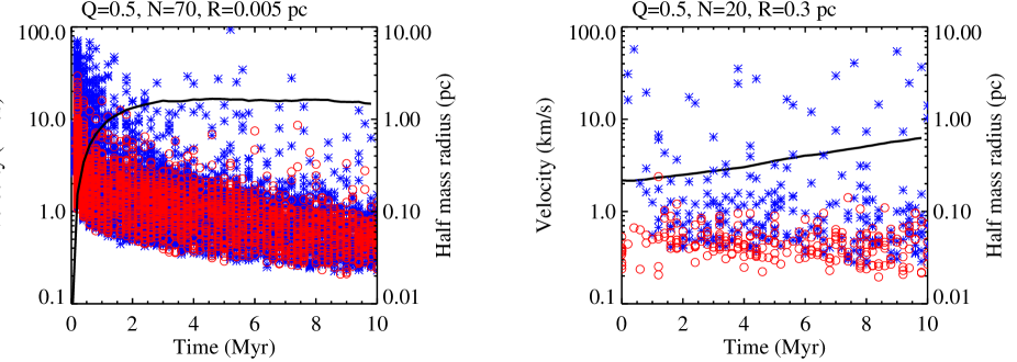
Figure 2: The left panel displays the velocity of ejected members at the time of ejection (blue asterisks for single objects, and red open circles for binaries) for a dense configuration from model A, with $N_{\text{sys}}=70$, $Q_{i}=0.5$, and $R_{\text{Pl}}=0.005$ pc. The right panel corresponds to a sparse configuration with $N_{\text{sys}}=20$, $Q_{i}=0.5$, and $R_{\text{Pl}}=0.3$ pc). The half mass radius evolution is superimposed (thick line), as a footprint of the stellar density for both cases.

This indicates that this criterion is very difficult to fulfil simultaneously with the other criteria. A dense initial state is necessary to remove all (or almost all) very low mass members from the cluster by enhancing two-body encounters, especially as more objects are released during the processing of wide binaries. However this tends to quickly inflate the inner core, acting in opposition to the criteria on the number of systems ($N_{1}$) and massive stars ($N_{2}$) and increasing the number of stars in the halo ($N_{3}$). This is illustrated for the dense initial configuration with {$N_{\text{sys}}=70$, $R_{\text{Pl}}=0.005$ pc, $Q_{i}=0.5$} in the left panel Fig.  2. There is a peak of cluster members ejection before 1 Myr with velocities as high as 60 km/s (especially for single objects released by binary decay). As an imprint of this highly dynamic phase the cluster undergoes a fast expansion phase, shown by the increase of the half mass radius from 0.01 pc to 1 pc within 1 Myr. Once the density has fallen off, the dynamics involves softer interactions (secular evolution) and the number of ejected members decreases along with their velocity. During this phase the cluster expands slowly until reaching virial equilibrium.
As a result of the fast relaxation phase the VLMOs are ejected efficiently but the numbers of systems ($N_{1}$) and massive stars ($N_{2}$) remaining in the cluster core are too small. In addition, the core expansion adds many solar-type systems to the halo, incompatible with the criterion $N_{3}$. We can move to a less dense initial state to try to improve the results, but then the expansion is too slow and the number of VLMOs inside a 2.6 pc radius ($N_{4}$) remains almost constant with time. When starting with a sparse configuration ($N_{\text{sys}}=20$, $R_{\text{Pl}}=0.3$ pc and $Q_{i}=0.5$ ), we do not see any peak of ejection at earlier times, and the half mass radius increases slowly and linearly in time (Fig. 2, right panel). It seems therefore that a compromise on the initial density has to be found in order to eject most of the VLMOs while retaining a dense enough core (compatible with criteria $N_{1}$ and $N_{2}$) and without populating the halo.
To better understand the cluster dynamical evolution, we show in Fig.  3 the evolution of the six quantities constrained by the observations for the 200 realizations that started with an intermediate density ($N_{\text{sys}}=40$, $Q_{i}=0.5$ and $R_{\text{Pl}}=0.05$ pc). The range corresponding to each criterion is delimited by solid lines in each panel.

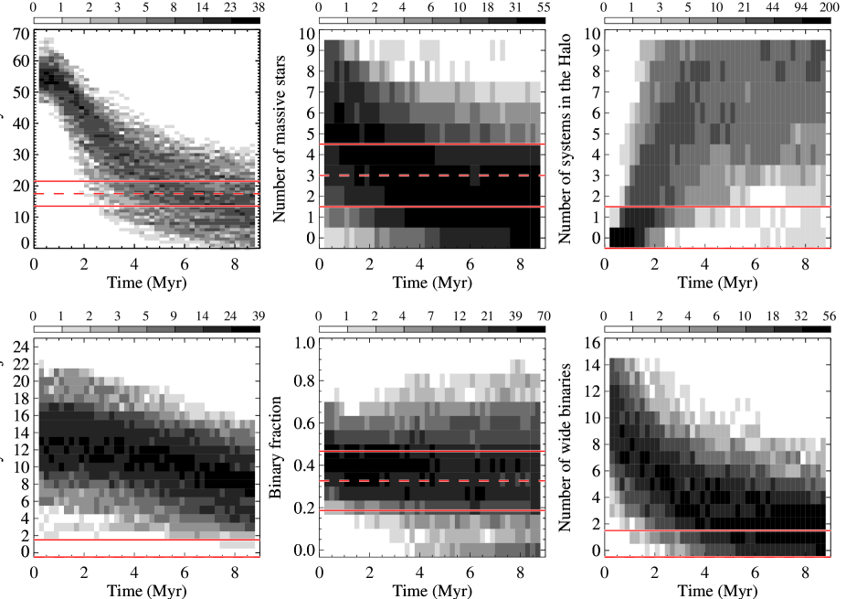
Figure 3: 3D histograms showing the evolution of (a) the number of systems in the core $N_{1}$, (b) the number of massive stars in the core $N_{2}$, (c) the number of systems in the halo $N_{3}$, (d) the number of VLMOs inside a 2.6 pc radius $N_{4}$, (e) the binary fraction in the core $N_{5}$, and (f) the number of wide (separation greater than $50$ AU) binaries $N_{6}$ as a function of time for model A and for the initial configuration {$N_{\text{sys}}=40$, $R_{\text{Pl}}=0.05$ pc, $Q_{i}=0.5$}. The histogram density corresponds to the number of simulations (out of 200) that fall in a given bin. The dashed and solid red lines correspond to the observed value and the acceptable range respectively.

First, it is interesting to note from the top left panel that the number of systems does not actually start at the setup value 40, but around 53 in average. This is mainly due to not counting bound pairs with separations larger than 400 AU as binaries but as two single objects, thus increasing the total number of systems. This can also be seen in the lower middle panel, where the binary fraction is initially around $46\%$, instead of 100% as set up. Then, during the cluster early evolution phase, binaries are processed more or less efficiently due to dynamical interactions, depending on their separation and on the initial density. In this case the binary fraction decreases from 46% to 43% within 0.5 Myr. As a consequence of the binary disruption the number of systems inside the inner core increases slightly during the first 0.5 Myr. After this phase, dynamical interactions are softer. The secular evolution tends to inflate the core, slowly dispersing the cluster members, decreasing the number of systems ($N_{1}$) and wide binaries ($N_{5}$) in the inner core, and increasing the number of stars in the halo ($N_{3}$).
The number of VLMOs inside a 2.6 pc radius ($N_{4}$) evolves in a similar way to the number of systems in the inner core (see bottom left panel). Note that the number of very low mass systems expected from the initial conditions (log-normal single star IMF, 100% binary fraction and random pairing) should be around 6 for $N_{\text{sys}}=40$. However, the number of VLMOs is already $\simeq 13$ at $t=0$ Myr (bottom left panel of Fig. 3), due to the fact that any very low mass ($m<0.1$ $\text{M}_{\odot}$) companion at separation larger than 400 AU is counted as a single object. This number remains constant during the first 0.5 Myr as binary disruption compensates for the ejection process. Then, later in the cluster evolution, the number of VLMOs ($N_{4}$) decreases slowly, as does the number of systems. However, it remains larger than five for most of the simulations starting with $N_{\text{sys}}=40$, $R_{\text{Pl}}=0.05$ pc and $Q_{i}=0.5$.
Overall, the success rate for the simulations to reproduce the observations is zero for all the initial configurations in model A.

5.2 Best-fitting initial conditions

In order to know which criterion is the most stringent and how the model hypothesis could be modified to reproduce $\eta$ Cha, we performed the analysis based on probability maps of $a_{i}(t_{i,m})$ described in section 4.2.

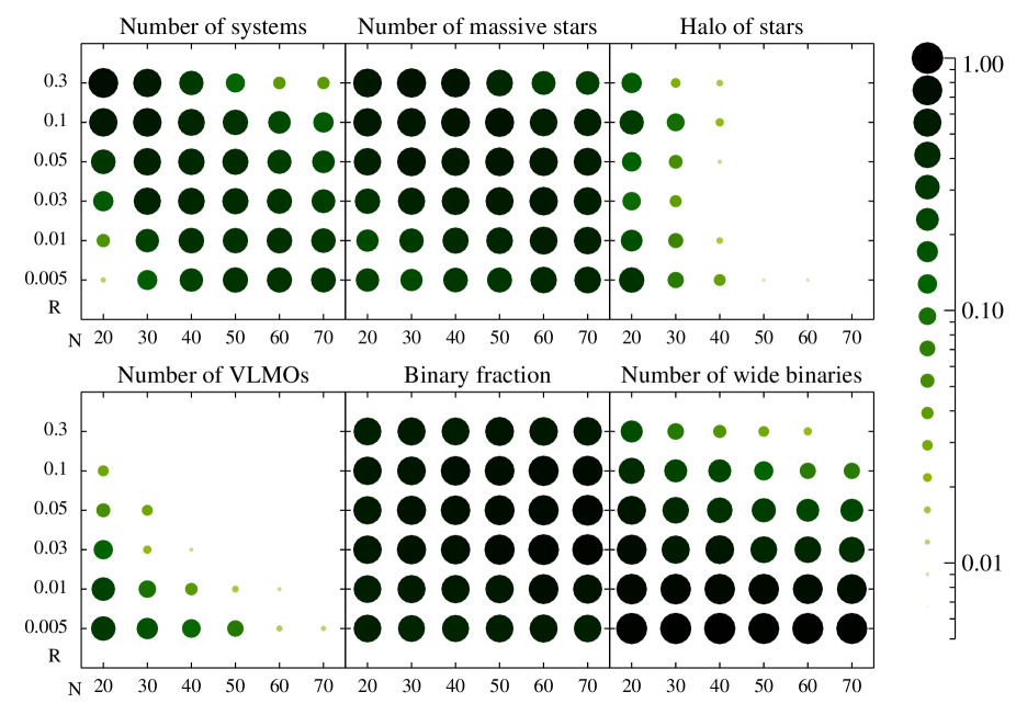
Figure 4: Summary for all tested configurations for model A with a virial ratio $Q_{i}=0.5$. For convenience the value for the quality measure, $a_{i}(t_{i,m})$ is also indicated by the dot size, with a logarithmic scale. For each criterion, the colour (and size) of the circles indicates the probability for the simulations to reproduce the observations. The results obtained with a different virial ratio $Q_{i}$ are very similar.

Fig. 4 reveals the regions (in {$N_{\text{sys}}$, $R_{\text{Pl}}$} coordinates, for $Q_{i}=0.5$) which most likely satisfy a given observational criterion. Below we review the inability of the simulations performed in model A to reproduce the observations, in the light of Fig. 4. Note that the time constraint is not mentioned, but was applied to produce all the discussed probability maps.

$N_{1}$

We notice that the probability to fulfil the criterion on the number of systems in the core drops if we start with large initial values for $N_{\text{sys}}$ and $R_{\text{Pl}}$ since the density becomes too small to remove enough systems from the inner core by dynamical interactions. On the other hand, when starting with a low $N_{\text{sys}}$ and $R_{\text{Pl}}$, the number of systems that remain in the core becomes rapidly too small.

$N_{2}$

The criterion on the number of massive stars seems to be easy to reproduce and does not strongly depend on the initial parameters although there is a small trend in favour of less dense cases or large value of $N_{\text{sys}}$.

$N_{3}$

Considering the number of systems in the halo, it is clear that this criterion is best matched with the smallest $N_{\text{sys}}$ because less objects can be ejected in the halo. For $N_{\text{sys}}=30$ or 40, this criterion is more easily fulfilled for either large $R_{\text{Pl}}$ (as lower density leads to fewer ejections), or small $R_{\text{Pl}}$ (as high density induces fast ejections, leading to large projected distances by 5 Myr). Intermediate values of $R_{\text{Pl}}$ result in too many slow-moving ejected stars that will remain in the vicinity of the cluster. For $N_{\text{sys}}>40$ the criterion on ($N_{3}$) is very badly reproduced for any value of $R_{\text{Pl}}$.

$N_{4}$

The result for the VLMOs is important since the region of agreement is very narrow. This shows that this criterion together with $N_{3}$, is the most stringent. It requires a low value of $N_{\text{sys}}$ to minimize the initial number of VLMOs to eject, and a low $R_{\text{Pl}}$ to maximize the dynamical encounters and eject these objects efficiently.

$N_{5}$ and $N_{6}$

We notice that the map for the binary fraction ($N_{5}$) does not indicate a large dependence on the parameters with an overall good agreement with the observations. The separation map ($N_{6}$) reveals a higher probability for the dense cases, which process the widest binaries and expand fast enough so that less binaries are present in the central region.

Although very narrow, the overlap region between the agreement maps of the various criteria (especially those for $N_{3}$ and $N_{4}$) seems to indicate that suitable initial configurations may be found (e.g see Fig. 4) for intermediate to low $N_{\text{sys}}$ and low $R_{\text{Pl}}$ (except for the lowest values for which the criterion on the number of systems $N_{1}$ is not well fulfilled). However this result is misleading for the criteria are not independent. There is a significant anti-correlation between the number of stars in a 10 pc halo ($N_{3}$) and the number of VLMOs in a 2.6 pc radius ($N_{4}$) at low and medium initial densities (as seen Fig. 5 for $N_{\text{sys}}=30$ and $R_{\text{Pl}}=0.05$ pc). In these cases the constraints on $N_{3}$ and $N_{4}$ tend not to be compatible. At higher densities and especially for $R_{\text{Pl}}=0.005$ pc, this anti-correlation becomes negligible. Both $N_{3}$ and $N_{4}$ get very small: the strong dynamical interactions remove all VLMOs from the core, and most ejected objects travel much further away than 10 pc within 5 Myr due to the high ejection velocities. However, the dynamical interactions are so strong that it is very difficult to retain anything in the cluster core and the number of systems $N_{1}$ becomes too small. Fig. 6 shows the correlation between $N_{1}$ and $N_{4}$ at $t=7$ Myr for the 200 simulations starting with $N_{\text{sys}}=30$ and $R_{\text{Pl}}=0.05$ pc. In all cases, when the number of VLMOs is less or equal to one, the number of systems in the core is smaller than 10, making these two criteria incompatible. We found a similar correlation for all the initial configurations tested by our simulations. The negative result of the previous analysis indicates that ejecting all VLMOs from the cluster core and keeping enough systems in a $0.5$ pc sphere is a major challenge.

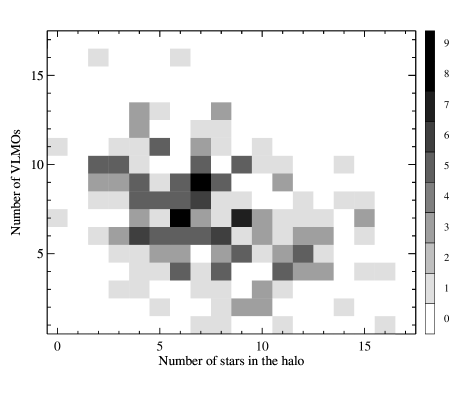
Figure 5: Correlation map between the number of VLMOs ($N_{3}$) and the number of solar-type stars in the halo ($N_{4}$) at $t=7$ Myr for $N_{\text{sys}}=30$, $R_{\text{Pl}}=0.05$ pc and $Q_{i}=0.5$ (model A).

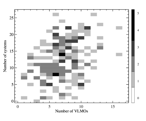
Figure 6: Correlation map between the number of systems ($N_{1}$) and the number of VLMOs ($N_{3}$) at $t=7$ Myr for $N_{\text{sys}}=30$, $R_{\text{Pl}}=0.05$ pc and $Q_{i}=0.5$ (model A).

The results obtained for different values of $Q_{i}$ (from 0.3 to 0.7) cannot be statistically distinguished from those obtained for the state initially in virial equilibrium ($Q_{i}=0.5$).

5.3 Summary and comparison with the previous study

Using standard initial conditions corresponding to model A, we tested many different configurations, varying the density and virial ratio. The main conclusions from this analysis are that

• starting with a single log-normal IMF with a peak value $\mu=0.2$ $\text{M}_{\odot}$ and a deviation $\sigma=0.55$, and assuming an initial binary fraction of 100%, random pairing and a Kroupa-like period distribution for the binary population, does not allow the simulations to reproduce the observations for any configuration {$N_{\text{sys}}$, $R_{\text{Pl}}$, $Q_{i}$};

• there is no hint of an improvement at the edge of the parameter grid, suggesting that our failure to find a solution is not a consequence of using a limited parameter space.

In Moraux et al. (2007b) the best fitting set of initial parameters gave a success rate of about 5%, whereas in our analysis of model A it is 0%. The apparent divergence between our results and Moraux’s is the consequence of the initial conditions. In the previous study, the chosen IMF corresponded to the system mass function obtained after binary processing (as it is observed in the field or in clusters), and binaries were considered as unbreakable objects, unable to exchange energy to the cluster by modifying their orbital properties. Here, the system IMF peaks at higher masses, generating more systems with mass $m>0.5$ $\text{M}_{\odot}$ initially, potentially increasing the number of them that could end up in the halo. This makes the criterion on $N_{3}$ more difficult to fulfil in the present study. Besides, binary disruption can significantly alter our ability to reproduce criterion $N_{4}$. Even though there are less very low mass systems initially, many objects with $m<0.1$ $\text{M}_{\odot}$  belong to a binary system with a separation larger than 50 AU or have been be released by binary decay. In both cases, these objects will be accounted for in the number of VLMOs ($N_{4}$), and this criterion is therefore not improved.

6 Alternative initial conditions

We discussed above the importance of the binary population in shaping the system IMF and hosting VLMOs that may be released in the cluster core. Since these processes depend strongly on the binary properties (mass ratio and separation distributions), we will now describe how they may be adjusted (model B and C) to better reproduce the observations. We will also discuss the possibility that the single star IMF might be discontinuous around the substellar limit (model D), which may help to reduce the initial number of VLMOs in the core. We will then present the results obtained in the extreme case when starting with an IMF truncated at 0.1 $\text{M}_{\odot}$ and a binary fraction of 100% (model E) or less (model F).

6.1 Binary pairing (Model B)

In model A, we chose for simplicity to pair binaries randomly from the same single IMF. Nevertheless, recent studies of both the galactic field (Raghavan et al. 2010; Reggiani & Meyer 2011) and star forming regions (Kraus et al. 2008, 2011) indicate that, whereas there is no clear and unique best fit, a flat mass ratio distribution may be a better fit than a random pairing.
Since this would result in a slightly smaller number of very low mass companions, we may expect the criterion on $N_{4}$ to be better fulfilled. To implement it in our initial conditions for model B, we sample the primary mass from a primary IMF and then draw the secondary mass according to a flat mass ratio distribution. This requires a slight change in the parameters of the primary IMF, in order to reproduce the log-normal single IMF. This gives $\mu=0.32$ $\text{M}_{\odot}$ and $\sigma=0.55$ (instead of $0.2$ $\text{M}_{\odot}$ and $0.55$ in case of random pairing). The binary fraction and separation distribution are the same as in model A.
We ran simulations for $Q_{i}=0.5$ only, $N_{\text{sys}}$=20 and $N_{\text{sys}}$=40, with the same range for $R_{Pl}$ as before. Results show that the agreement probability on the number of VLMOs ($a_{4}$) is larger (by a factor of two to three), contrary to the probability $a_{3}$ on the halo that is smaller (by a factor of about 2). This is due to the shift towards higher masses of the primary MF yielding more objects with $m>0.5$ $\text{M}_{\odot}$ that may end up in the halo. Overall, no significant improvement is observed when using a flat mass ratio distribution since again no simulation is able to reproduce the observations.

6.2 Separation distribution (Model C)

In the following, we discuss the possibility that no wide binary formed initially by assuming an initial separation distribution similar to model A but truncated at large separation. The cut-off separation value and the initial binary fraction are linked to each other and we explain below how they can be evaluated providing the final binary fraction.
Following the simplistic argument that all binaries with a separation smaller than a given value (hard binaries) survive throughout the simulation, and that any wider binary is destroyed, we can express the initial binary fraction $f_{b}$ in terms of the initial hard binary fraction $f_{hb}=N_{hb}/N_{b}$ (where $N_{b}$ is the number of binaries and $N_{hb}$ the number of hard binaries) and the final binary fraction $f^{\prime}_{b}$:

$$f_{b}=\frac{f^{\prime}_{b}}{(1+f^{\prime}_{b})f_{hb}-f^{\prime}_{b}}$$ (1)

Taking a final binary fraction of 36% given by the observations, we consider different values of $f_{b}$, ranging from 36% to 100%. The corresponding initial hard binary fraction ranges from 100% (all binaries survive) to 53% (about half the binaries survive) respectively. To follow the observations, we identify as hard binaries (that will not be destroyed) those with separations lower than 50 AU. From the initial hard binary fraction, we then estimate the corresponding separation cut-off, assuming a Kroupa (1995b) distribution below this value. For example, we need a cut-off at 730 AU for a hard binary fraction of 53%. The lowest possible cut corresponds naturally to 50 AU, to get 100% hard binaries. Fig. 7 illustrates this process in the case of an initial binary fraction of $f_{b}=0.8$, which gives $f_{hb}=0.6$. This initial hard binary fraction is obtained when applying a cut-off in the separation distribution around 370 AU.

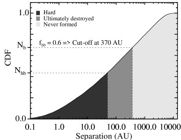
Figure 7: Cumulative separation distribution function (solid line) obtained from the Kroupa period distribution (see section 3). This highlights how the distribution is truncated in Model C in the case of $f_{b}=0.8$. Expression 1 yields $f_{hb}=0.6$, which imposes to truncate the separation distribution to 370 AU, so that $N_{hb}=0.6\times N_{b}$.

Table 5: Binary fraction and separation cut-off for model C.

$f_{b}$ (%)	100	90	80	70	60	50	40
Cut-off (AU)	730	570	370	240	150	90	50

We can wonder why these binary properties would result from the cluster formation process and this needs to be compared to what is observed in star forming regions. In dense environment such as the Trapezium $f_{b}\simeq$ 60%, whereas in sparse regions like Taurus $f_{b}\simeq$ 90% (Duchêne 1999; Kirk & Myers 2012). A plausible explanation for this difference is that all star forming regions start their evolution with a high binary fraction and the wide binaries are further disrupted in dense environments within 1 Myr (see e.g Marks & Kroupa 2012). In the Trapezium, very few binaries with a separation larger than 1000 AU have been found (Scally et al. 1999) which supports this idea. For instance it was possible to reproduce the evolution of the ONC (Kroupa et al. 2001; Marks & Kroupa 2012) starting with 100% binaries and a density of $10^{5}$ stars/pc³, including the deficit of [200-500] AU binaries compared to the separation distribution for field binaries from Raghavan et al. (2010) (Reipurth et al. 2007). In our simulations starting with $N_{\text{sys}}=20$ and $R_{Pl}=0.05$ pc, the initial density is very similar ($2\times 10^{5}$ stars/pc³). However, the adopted separation cut-off at 50 or 90 AU cannot be explained by dynamical encounters since these separation limits are much lower than the initial mean neighbour distance (around 2200 AU). Nevertheless, it is still possible that the binary fraction may be set up during the formation process and/or during the gas-rich phase which is not covered in our simulations.
We ran the simulations for $Q_{i}=0.5$, $N_{\text{sys}}=20$ to 70, and $R_{Pl}=0.005$ pc to 0.3 pc (model C). The parameters used for the binary fraction and separation cut-off are given in Table 5. A flat mass ratio distribution (as in model B) has been used to generate the secondary masses.
Fig. 8 shows the evolution of the probability $a_{i}(t_{i,m})$ in the case $N_{\text{sys}}=20$ and $R_{Pl}=0.1$ pc for the six criteria as a function of the adopted separation cut-off. For a large separation cut-off, the probability of agreement for the binary fraction is low ($<0.2$). This is worse than what was obtained for models A and B, for which no cut-off was applied to the Kroupa-like separation distribution. This is because (1) more binaries have a separation lower than $400$ AU and are thus identified as binaries in the analysis procedure leading to a higher initial binary fraction, and (2) the high binary fraction remains almost constant in time, unless the initial density is very high. An improvement is naturally seen for the criteria on the binary fraction as well as on the number of wide binaries when the separation limit gets smaller ($<100$ AU). Applying a cut-off at 50 AU corresponds to removing the constraints on the binary population since we already start with what is observed (no wide binaries and $f_{b}=40$%). The probability $a_{3}$ for the halo is also increasing, from 0.08 to 0.4 for the lowest cut-off. For the number of systems ($N_{1}$), the number of massive stars ($N_{2}$), and the number of VLMOs ($N_{4}$) the probability does not change significantly. This may be surprising at first, especially for $N_{4}$, as less VLMOs will be produced by binary decay. However, this effect is compensated by the slower dynamics making it more difficult to eject the VLMOs from the core even though they are less numerous.
Nevertheless, the analysis reveals two configurations ($Q_{i}=0.5$, $N_{\text{sys}}=20$, and $R_{Pl}=0.05$ pc and 0.1 pc) for which some simulations satisfy all criteria if the separation cut-off is 50 AU. We found respectively one and three simulations out of 200 that fulfil all the observational constraints.

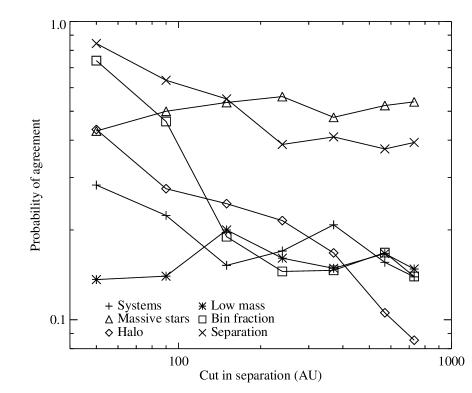
Figure 8: Evolution of the agreement probability for the different criteria, when setting a maximum value for the binary separation, varying from 50 to 730 AU, and adopting a flat mass-ratio distribution (model C). The results are given for {$Q_{i}$=0.5, $N_{\text{sys}}$ = 20, $R_{pl}$ = 0.1 pc}.

To check whether these successful runs are consistent with the recent results from Murphy et al. (2010), we look at the number of low mass systems in the mass range [0.08, 0.3] $\text{M}_{\odot}$ located at a distance range [2.6, 10] pc from the cluster centre. We find between zero to one of these systems, which is possibly too small compared to the detection of four probable plus three possible candidates.

6.3 Treating brown dwarfs as a separate population (Model D)

So far we have considered a continuous IMF that extends to the substellar regime (down to $0.01$ $\text{M}_{\odot}$), but Thies & Kroupa (2007) suggest that brown dwarf (BD) formation may be different to star formation (based on their binary properties), which would lead to a discontinuous mass distribution for single objects. This assertion is still a matter of debate, but nonetheless finds observational support from the mass function of young star clusters (Thies & Kroupa 2008) and BD binaries surveys (Kraus & Hillenbrand 2012). Parker & Goodwin (2011) excluded pure dynamical evolution as a possible explanation for the observed differences between the separation distributions of stellar and substellar binaries, implying that it may be a pristine feature (or set during the very early evolution). From a theoretical point of view, the process of BD formation remains unclear and may involve a star-like collapse within a turbulent medium (e.g. Whitworth & Stamatellos 2006) or a more specific channel of early ejection of gaseous clumps (Reipurth & Clarke 2001; Basu & Vorobyov 2012). Other plausible mechanisms suggest massive disc fragmentation (Stamatellos et al. 2007) or gravitational instabilities induced in disks as a result of encounters in embedded clusters (Thies et al. 2010).
To evaluate the possibility that the single IMF may be discontinuous (model D), we consider initial conditions corresponding to the results from Thies & Kroupa (2008). We adopted two log-normal single mass functions with $\mu=0.08$ $\text{M}_{\odot}$  and $\sigma=0.69$, but one corresponds to stars and is limited to the mass range [0.07, 4] $\text{M}_{\odot}$ and the other one corresponds to BDs and very low mass stars (VLMS) with $0.01<m<0.15$ $\text{M}_{\odot}$. There is an overlap between the two mass functions in order to end up with a continuous system IMF consistent with the universal picture of the IMF. Each population (stars, and BDs + VLMSs) is treated separately and the BDs and VLMSs to stars ratio is assumed to be $1/5$. The BD and VLMS binary fraction and the star binary fraction are respectively 30% and 100% and there are no mixed BD/VMLs binaries (Kroupa et al. 2011). For simplicity we generate the binaries for each population using random pairing and the same period distribution with no separation cut-off. The latter hypothesis is not realistic since field BD binaries are known to have a tighter period distribution (Burgasser et al. 2007) that cannot be explained by pure dynamical evolution (Parker & Goodwin 2011). Nevertheless this will have a very limited impact on our results, since the number of BD binaries is one or two in average (if starting respectively with $N_{\text{sys}}=20$ or $N_{\text{sys}}=40$).
We ran simulations in the virialized case for $N_{\text{sys}}=20$ and $R_{\text{Pl}}$ within {0.05, 0.1} pc as well as for $N_{\text{sys}}=40$ and $R_{\text{Pl}}=0.05$ pc. As a result of the analysis the improvement over our previous simulations is limited: no simulation matches all observations of the $\eta$ Cha cluster. Compared to the standard case (model A), the main improvement lies in the probability $a_{3}$ to reproduce the halo, which is mainly explained by the shift towards lower masses of the system IMF. At best the probability increases from 0.29 to 0.55 in the case with $N_{\text{sys}}=20$ and $R_{\text{Pl}}=0.1$ pc. Note that this probability is also higher than when we applied a separation cut-off at 50 AU (model C, see Fig.8). However, the probability of agreement for the criterion on the VLMOs decreased compared to the result from model A (from 0.03 to 0.005 for $N_{\text{sys}}=20$ and $R_{\text{Pl}}=0.1$ pc). We can understand this by counting the mean number of VLMOs at t=$0.6$ Myr, after the binary breaking phase: for $N_{\text{sys}}=20$ and $R_{\text{Pl}}=0.1$ pc we find $N_{VLMO}=8$, compared to $N_{VLMO}=6.5$ in the standard case (model A) and to $N_{VLMO}=4.2$ in the extreme case of model C starting with $40$% binaries and a cut-off at $50$ AU in separation. Since the number of VLMOs is a strong constraint, this comparison shows the limited effect of the changes adopted for the BD population.

6.4 Truncated IMF at the low mass limit and truncated separation distribution (Models E and F)

The previous analysis indicates that the observational result regarding the number of VLMOs in $\eta$ Cha is particularly difficult to reconcile with the other constraints, in particular with the number of systems in the core and the absence of solar-type star in the halo (see Fig. 5 and 6). In the following we consider the extreme scenario where the IMF is not universal and no very low mass system ($m<0.1$ $\text{M}_{\odot}$) has formed initially. To do so, we generate primary masses from the same primary IMF (peaking at $0.3$ $\text{M}_{\odot}$) as in model B, but truncated at $0.1$ $\text{M}_{\odot}$, and use a flat mass ratio distribution (without any truncation on the secondary mass)
We first ran simulations starting with a virialized Plummer sphere with 100% binaries drawn from the Kroupa separation distribution (model E). $N_{\text{sys}}$ and $R_{\text{Pl}}$ are chosen within {20, 30, 40, 50, 60} and {0.005, 0.01, 0.03, 0.05, 0.1, 0.3} pc respectively. We discarded the larger value $N_{\text{sys}}=70$ since it would give a cluster starting with too many systems to fulfil the criteria on the number of systems in the inner core without populating the halo. As a result no simulation fulfilled all 6 criteria. This as an outcome of both the truncation itself and the choice for the initial binary fraction of 100%. Because of the lower mass limit the initial number of stars with $m>0.5$ $\text{M}_{\odot}$ increases for a given $N_{\text{sys}}$, making the criterion on the halo more difficult to reproduce. In addition, since there is no truncation in the secondary mass distribution, a few VLMOs are part of a binary system and will appear as single objects, either because their separation is larger than 400 AU or because the binary will be processed by dynamical evolution. For instance, in the case $N_{\text{sys}}=20$ and $R_{\text{Pl}}=0.1$ pc, $2.5$ VLMOs are identified in average at $t=0$ Myr. As a consequence the criteria on the VLMOs and on the halo remain difficult to fulfil together with the other criteria.
We ran additional simulations (model F) where we introduced a cut-off in the initial binary period distribution in a similar way as for model C (see section 6.2). We find that when starting with a binary fraction of 40% and a cut-off at 50 AU many more simulations could reproduce the six observational constraints with a success rate up to 10% for $N_{\text{sys}}=20$ and $R_{\text{Pl}}=0.1$ pc. The average number of VLMOs in this initial configuration is $0.2$ at $t=0$ Myr, which shows that the constraint on the number of VLMOs is easily satisfied, given that there are only close binaries (with separation $<50$ AU) that very stable dynamically. It is interesting to note that the very few runs of model C that are also able to reproduce all the criteria correspond to the same initial conditions. Indeed the successful cases were obtained for $N_{\text{sys}}=20$ and $R_{\text{Pl}}=0.05$ or 0.1 pc and started with only one or two VLMOs initially. This seems to indicate that both the IMF and the initial binary population of $\eta$ Cha were not standard.
When considering Murphy’s constraint however, the success rate shrinks to 0.5% at best, if we require to have at least three stars in the mass range [0.08; 0.3] $\text{M}_{\odot}$ and within a 10 pc radius. Despite a low success rate, this model is the only one that can reproduce all the observational constraints, including Murphy’s results. Note that the only successful runs are for two medium density configurations: {$N_{\text{sys}}=30$; $R_{\text{Pl}}=0.1$ pc} and {$N_{\text{sys}}=30$; $R_{\text{Pl}}=0.05$ pc}.

7 Summary and conclusion

We have conducted a large set of pure N body simulations that aim to reproduce the peculiar properties of the $\eta$ Cha association, namely the lack of very low mass objects ($m<0.1$ $\text{M}_{\odot}$) and the absence of wide binaries (with a separation $>50$ AU). We tested several models of various IMF and binary properties, and span the parameter space in density and virial ratio. The analysis was done using several procedures in order to compare efficiently the simulation results with the observational data and identify the best initial state.
In order to test a universal picture for the IMF, we assumed a continuous log-normal single IMF with $\mu=0.2$ $\text{M}_{\odot}$and $\sigma=0.55$. Starting with this IMF and a binary fraction of 100% (with either a random pairing, model A, or a flat mass ratio distribution, model B), the analysis shows that ejecting all very low mass members without creating a halo of solar-type stars and keeping an inner core of 18 systems is not possible. Similarly to the case of a discontinuous single IMF, no simulation was able to match the observations.
Reproducing all available observations of $\eta$ Cha by pure dynamical evolution from an universal single IMF and a stellar binary fraction of 100% is therefore very unlikely.
We then tested a different set-up for the binary population, while preserving the shape of the IMF, our working hypothesis (model C). We assumed that wide binaries do not form initially and adopted a separation distribution truncated at large separation resulting in a lower binary fraction. As a result, the best initial state, starting with an initial binary fraction of 40% binaries and without any binary wider than 50 AU, yields a small success rate of 1% (that drops to 0% if we require those simulations to have a halo of ejected low mass stars (Murphy et al. 2010)). Since almost no considered initial state assuming a universal IMF statistically matches the observational constraints, we started with a truncated IMF with no system below 0.1 $\text{M}_{\odot}$. However, this fails in reproducing the observations, unless starting with a singular binary population (no wide binary and a small binary fraction; model F). In this case, the best success rate is 10% and is obtained for initial parameters ($N_{\text{sys}}=20$ and $R_{\text{Pl}}={0.1;0.05}$ pc) that are very similar to what is observed today in the cluster.
This suggests that the dynamical evolution did not play a strong role in shaping the properties of $\eta$ Cha and that most of them must be pristine. $\eta$ Cha may have started with an IMF deficient in VLMOs and with peculiar binary properties (namely a small binary fraction and an orbital period distribution truncated at small periods). Note that this conclusion is very different from Moraux et al. (2007b) where the initial high density case was the preferred solution. This stresses the importance of the binary population in the overall dynamical evolution of the cluster.
One can speculate onto the particular physical conditions that might have produced so few VLMOs together with preventing wide binaries from forming. $\eta$ Cha may for instance originate from a highly magnetized cloud, preventing fragmentation of large scale (Hennebelle et al. 2011), forcing more mass into single fragments and not creating wide systems. Tighter binaries could then be produced later on, after the magnetic field has diffused out.
Finally, in the low density case solution presented above, it is very difficult to reproduce the recent results from Murphy et al. (2010). When considering this additional constraint, the success rate becomes very small (0.5% at best). Additional knowledge of the kinematics of this purported halo population might help refine the dynamical picture of $\eta$ Chamaeleontis.