The Einstein@Home search for radio pulsars and PSR J2007+2722 discovery

Abstract

Einstein@Home aggregates the computer power of hundreds of thousands of volunteers from 193 countries, to search for new neutron stars using data from electromagnetic and gravitational-wave detectors. This paper presents a detailed description of the search for new radio pulsars using Pulsar ALFA survey data from the Arecibo Observatory. The enormous computing power allows this search to cover a new region of parameter space; it can detect pulsars in binary systems with orbital periods as short as 11 minutes. We also describe the first Einstein@Home discovery, the 40.8 Hz isolated pulsar PSR J2007+2722, and provide a full timing model. PSR J2007+2722’s pulse profile is remarkably wide with emission over almost the entire spin period. This neutron star is most likely a disrupted recycled pulsar, about as old as its characteristic spin-down age of 404 Myr. However there is a small chance that it was born recently, with a low magnetic field. If so, upper limits on the X-ray flux suggest but can not prove that PSR J2007+2722 is at least $\sim 100$ kyr old. In the future, we expect that the massive computing power provided by volunteers should enable many additional radio pulsar discoveries.

1. Introduction

Einstein@Home is an on-going volunteer distributed computing project (Anderson et al., 2006), launched in early 2005. More than 330 000 members of the general public have “signed up” their laptop and desktop computers. When otherwise idle, these computers download observational data from the Einstein@Home servers, search the data for weak astrophysical signals, and return the results of the analysis. The collective computing power is on par with the largest supercomputers in the world.

The goal of Einstein@Home is to discover neutron stars, using data from an international network of gravitational-wave (GW) detectors (Sathyaprakash & Schutz, 2009), from radio telescopes (Lyne & Graham-Smith, 1998; Lorimer & Kramer, 2004), and from the Large Area Telescope (LAT; Atwood et al., 2009) gamma-ray detector onboard the Fermi Satellite. Because the expected signals are weak, and the source parameters are unknown, the sensitivity of the GW searches (Brady et al., 1998; Brady & Creighton, 2000) the radio pulsar searches (Brooke et al., 2007), and the gamma-ray searches (Pletsch & Allen, 2009; Pletsch et al., 2012b, c, a) are limited by the available computing power.

Before 2009, Einstein@Home only searched data from the Laser Interferometer Gravitational-Wave Observatory (LIGO; Abramovici et al., 1992; Barish & Weiss, 1999; Abbott et al., 2009c). So far these searches have not found any sources, but have set new and more sensitive upper limits on possible continuous gravitational-wave (CW) emissions (Abbott et al., 2009a, b; Aasi et al., 2013). These searches are ongoing, with increasing sensitivity arising from improved data analysis methods (Pletsch & Allen, 2009) and better-quality data (Smith & LSC, 2009).

In 2009, Einstein@Home also began searching radio survey data from the 305-meter Arecibo telescope in Puerto Rico. This is the world’s largest and most sensitive radio telescope, and has discovered a substantial fraction of all known pulsars. Beginning in 2010 December a similar search using data from Parkes Observatory in Australia was also started; the differences from the Arecibo search and some results are described in Knispel et al. (2013).

Starting in summer 2011, Einstein@Home also began a search for isolated gamma-ray pulsars in data from the Fermi satellite’s LAT Atwood et al. (2009); this will be described in future publications.

The Arecibo data are collected by the Pulsar ALFA (PALFA) Consortium using the Arecibo L-band Feed Array (ALFA). For the pulsar survey, ALFA output is fed into fast, broad-band spectrometers (see Section 3.2); further down the data analysis pipeline (see Section 4.1) this enables compensation for the dispersive propagation of pulses from celestial sources.

The computing capacity of Einstein@Home is used to search the spectrometer output for signals from neutron stars in short-period orbits around companion stars. This is a poorly-explored region of parameter space, where other radio-pulsar search pipelines lose much or most of their sensitivity. The detection of these pulsars with standard Fourier methods is hampered by Doppler smearing of the pulsed signal caused by binary motion during the survey observation (Johnston & Kulkarni, 1991).

Previous searches (Anderson et al., 1990; Camilo et al., 2000) have utilized “acceleration searches” (Johnston & Kulkarni, 1991), which correct for the part of the binary motion which can be modeled as a constant acceleration along the line-of-sight. These computationally-efficient techniques are effective when the observation time is short compared to the orbital period. Thus, they are insensitive to the most compact systems (Ransom et al., 2002). In contrast, the computing power of Einstein@Home enables a full demodulation to be carried out, giving substantially increased sensitivity to signals from pulsars in compact circular orbits with periods below $\sim 1$ hr.

In 2010 August, Einstein@Home announced its first discovery of a new neutron star (Knispel et al., 2010) which appears to be the fastest-spinning “disrupted recycled pulsar” (DRP) so far found (Belczynski et al., 2010). In the same month, Einstein@Home also discovered a 48 Hz pulsar in a binary system (Knispel et al., 2011). Further Einstein@Home discoveries in Parkes Multi-Beam Pulsar Survey (PMPS) are described in Knispel et al. (2013). As of 2013 January, Einstein@Home has discovered almost 50 radio pulsars.

This paper has two purposes. First, it provides a full description of the Einstein@Home radio pulsar search and post-processing pipeline. Second, it provides a detailed description and full timing solution for the first Einstein@Home discovery, the 40.8 Hz pulsar PSR J2007+2722 (Knispel et al., 2010).

The paper is structured as follows. Section 2 presents a general description of the Einstein@Home computing project, including its motivation, its history, and its technical design and structure. Section 3 is an brief overview of the PALFA survey, including its history, the data taking rates, and data acquisition system. Section 4 is a detailed technical description of the Einstein@Home search for radio pulsars, starting from the centralized data preparation, through the distributed processing on volunteers’ computers, and centralized post-processing. Section 5 describes the discovery of the first Einstein@Home radio pulsar, PSR J2007+2722. Section 6 is about the subsequent follow-up investigations and studies, including observations at multiple frequencies, and accurate determination of the sky position through gridding and timing. We also discuss the evolutionary origin of PSR J2007+2722. This is followed in Section 7 by a short discussion and conclusion.

Unless otherwise stated, all coordinates in this paper are in the J2000 coordinate system, and $c$ denotes the speed of light.

2. The Einstein@Home Distributed Computing Project

2.1. Volunteer Distributed Computing

The basic motivation for volunteer distributed computing is simple: the aggregate computing power owned by the general public exceeds that of universities, and public and private research laboratories, by two to three orders-of-magnitude. Scientific research whose progress is limited or constrained by computing can benefit from access to even a small fraction of these resources. This type of research includes both numerical simulation and Monte-Carlo-type exploration of parameter spaces, that make no (direct) use of observational data, and data-mining and data-analysis efforts which perform deep searches through (potentially very large) observational data sets.

Worldwide, there are more than one billion personal computers (PCs) which are connected to the Internet. These PCs typically contain x86-architecture central processor units (CPUs) and substantial disk-based and solid-state storage. Many of these systems also contain graphics processor units (GPUs) which can perform floating point calculations one to two orders-of-magnitude faster than a modern CPU core.

The raw computational capacity of each of these consumer computers is similar to that of the systems used as building blocks for computer clusters or research supercomputers. In fact modern research computers are made possible only by the economies of scale of the consumer marketplace, which ensures that the basic components are inexpensive and widely available. But research machines typically consist of hundreds or thousands of these CPUs; volunteer distributed computing offers access to hundreds of thousands or millions of these CPUs.

2.2. Constraints on Suitable Computing Problems

Volunteer distributed computing is only a suitable solution for some computing and data analysis problems: there are both social and technical constraints. To attract volunteers, the research must resonate with the “person in the street”. It must have clear and understandable goals that appeal to the general public and that excite and maintain interest. Experience shows that at least four areas have these qualities: medical research, mathematics, climate/environmental science, and astronomy and astrophysics.

The technical constraints arise because the computers are only connected by the public Internet. This is very different than research supercomputers, which typically have low-latency high-speed networks which enable any CPU to access data from any other CPU with nanosecond latencies and GB/s bandwidth. In contrast, the latency in volunteer distributed computing can be fifteen orders-of-magnitude larger; a volunteer’s computer may only connect to the Internet once per week! The average available bandwidth is also much smaller, particularly for data distributed from a central (project) location. For example if a project is distributing data through a 1Gb/s public Internet connection to 100k host machines, the average bandwidth available per host is 10 kb/s, six orders-of-magnitude less than for a research facility.

The main technical constraints on the computing problem are therefore as follows:

(1.) It must lie in the class of so called “embarrassingly parallel” problems, whose solution requires no communication or dependency between hosts.

(2.) It must have a high ratio of computation to input/output. For example if the project distributes data through a single 1Gb/s network connection, and the application requires 1 MB of data per CPU-core-hour, then at most 360k host CPU-cores can be kept fully-occupied on a $24\times 7$ (round-the clock) basis.

(3.) It must use only a small fraction of available RAM (say 100 MB) so that the operating system (OS) can quickly swap tasks, providing normal interactive computer response for volunteers.

(4.) It must be capable of frequent and lightweight checkpointing (saving the internal state for later restart) using only a small amount of total storage (say 10 MB), so that it can snatch idle compute cycles but stop processing when the volunteer is using the computer or turns the computer off.

(5.) The code that will run on volunteer’s hosts must be mature enough to be ported to several different OSs, and to run reliably on volunteers computers.

In short, volunteer distributed computing is not a panacea: it can only be used to solve some computing problems.

2.3. Trends in Computing Power and GPUs

The latest trend in computing is the move to systems containing large numbers of processing cores. This is largely in response to the fundamental physical limits that arise in manufacturing integrated circuits. For more than 40 yr, the computing power available at fixed cost has doubled every 18 months. This was a consequence of “Moore’s law”, a heuristic observation that the number of components on an integrated circuit grew exponentially with time. This trend was made possible by the shrinking of the “process size” (the size of the smallest components on an integrated circuit) along with a corresponding increase in clock speed and a decrease in operating voltage. Operating voltages can no longer be decreased because they have approached the band-gap energy, and process sizes, currently at 22nm, have been shrinking more slowly than in the past. They are expected to decrease to about 10nm, but can not get much smaller; the inter-atomic spacing in a silicon lattice is 0.7nm. To get more computing power at reasonable cost, the only approach is to put large numbers of cores onto a single chip.

Fortunately the consumer marketplace has a demand for such systems: they are called GPUs and are used for high-quality rendering of graphics and video. The evolution of television from radio broadcasting to transmission over the Internet is now underway, and it is expected that over the next decade this will be an important driving force behind further growth in Internet capacity and graphics capability in consumer computers. Already more than 25% of Einstein@Home host machines contain GPUs, and we expect that this will approach 100% within the coming three years.

Current-generation GPUs have 500 or more cores, each capable of simultaneously doing one floating-point addition and one floating-point multiplication per clock cycle. The two leading manufacturers of such systems (NVIDIA and AMD/ATI) both provide application programming interfaces (APIs) that permit GPUs to be used for general-purpose computing. Thus, over the coming decade, if GPU capacity is accessed and exploited, volunteer distributed computing should continue to provide “Moore’s law scaling” and to provide access to more computing cycles than more traditional approaches.

In the longer-term, tablet devices and smartphones will probably provide the bulk of the computing power. Their CPUs and GPUs are very power-efficient, though typically an order-of-magnitude slower than laptop or desktop computers. However very large numbers are being marketed and used. These devices are often idle while connected to charging stations; during this time they represent a significant computing resource.

2.4. The Einstein@Home Project

Einstein@Home was formally launched at the American Association for the Advancement of Science meeting on 2005 February 19, as one of the cornerstone activities of the World Year of Physics 2005 (Stone, 2004). Members of the general public, whom we refer to as “volunteers”, “sign up” by visiting the project Web site http://einstein.phys.uwm.edu and downloading a small executable, which is available for Windows, Mac and Linux platforms. It takes a couple of minutes to install on a typical home computer or laptop (which is then technically refereed to as a “host”). After that, when the host is otherwise idle, it downloads observational astrophysics data from one of the Einstein@Home servers, and analyzes it in the background, searching for signals. The results of the analysis are automatically uploaded to a project server, and more work is requested. The system is designed to operate without further attention from the volunteer, although it is also highly configurable and can be tuned for specific needs if desired. The collective computing power is on par with the largest supercomputers in the world.

The Einstein@Home project also incorporates additional features intended to attract, inform, motivate and retain volunteers. These include message boards where volunteers can exchange messages with other volunteers and project personnel and scientists; granting computing credits as a symbolic “reward” for successful computing work; the ability to form teams to compete for computing credits; informational Web pages describing the science and results; and access to dynamic Web pages that allow volunteers to track the individual computing jobs done by their computers.

There are a number of such volunteer computing projects world-wide. They search for signs of extra-terrestrial life (SETI@Home, Anderson et al. (2002)), study protein-folding (Folding@Home, Shirts & Pande (2000)), search for new drugs (Rosetta@Home, Cooper et al. (2010)), search for large Mersenne prime numbers (GIMPS), simulate the Earth’s climate evolution (ClimatePrediction.net, Stainforth et al. (2005)) and so on.

Einstein@Home is one of the largest of these projects; to date, hosts registered by more than 330 000 people have returned valid results to Einstein@Home and have delivered more than one billion CPU hours. There are Einstein@Home volunteers from all 193 countries recognized by the United Nations; currently, more than 100 000 different computers, owned by more than 55 000 volunteers, contact the Einstein@Home servers each week, requesting work and uploading results.

The aggregate computing power of Einstein@Home is shown in real-time on a public server status page. As of 2013 January, it delivers an average of more than one Petaflop of computing power; according to the current (2012 November) Top-500 list, there are only 23 computers on the planet which can deliver more computing power on a peak basis (the time-average is necessarily lower). To help understand the scale, it is useful to provide some cost comparisons. Simply providing the electrical power needed to support this amount of computation would cost three to six million U.S. dollars per year. The costs of hardware and administration would be substantially greater. (Note: at the time of the PSR J2007+2722 discovery in 2010 August, there were about 250 000 registered volunteers, and Einstein@Home delivered about 200 Tflops of computing power.)

The original and long-term goal of Einstein@Home is to search GW data to find the continuous-wave signals emitted by rapidly-rotating neutron stars. The search is an integral part of the coordinated world-wide effort to make the first direct detections of GWs. These were predicted by Einstein in 1916, but have never been directly detected. A new generation of instruments, the LIGO in the USA, VIRGO in Italy, GEO in Germany, and the KAGRA Large-Scale Cryogenic Gravitational-Wave Telescope Project in Japan, offers the first realistic hopes of such a detection. GWs produced by rapidly spinning neutron stars are one of the four main targets for these detectors, but because the signals are weak, and the source parameters (sky position, frequency, spin-down rate, and so on) are not known, the sensitivity of the search is limited by the available computational power (Brady et al., 1998; Brady & Creighton, 2000).

Einstein@Home has carried out and published the most sensitive “blind” all-sky searches using data from the best GW detectors. While these searches have not yet detected any signals, they continue to be a principal target of the project. Upper limits obtained from Einstein@Home have been published using data from the LIGO instrument’s fourth and fifth science runs (S4 and S5; Abbott et al., 2009a, b; Aasi et al., 2013). Einstein@Home is also re-searching the full S5 and S6 data sets using a new method that has been proved optimal, for conventional assumptions about the nature of the instrumental and environmental noise sources (Pletsch & Allen, 2009; Pletsch, 2010, 2011).

Since 2009, Einstein@Home has also been searching electromagnetic data from the Arecibo Observatory, looking for radio pulsars in short-period orbits around companion stars. As explained in Section 1, this is an unexplored region of parameter space, where existing search methods lose much or most of their sensitivity.

Searches for binary radio pulsars can be characterized by the ratio of phase-coherently analyzed observation time $T$ to orbital period $P_{\text{orb}}$ of the pulsar. There are three cases. (1) For orbital periods long compared to the observation time, i.e. $T/P_{\text{orb}}\lesssim 0.1$, the signal can be well described assuming a constant acceleration and “classical” acceleration searches are a computationally efficient analysis method (Ransom et al., 2002) with only small sensitivity losses. (2) If multiple orbits fit into a single observation, i.e. $T/P_{\text{orb}}\gtrsim 5$, then sideband searches, defined in Ransom et al. (2003), provide a computational short-cut with a factor two to three loss in sensitivity (Jouteux et al., 2002; Ransom et al., 2003) compared with the optimal matched filter coherent search. (3) The intermediate range $0.1\lesssim T/P_{\text{orb}}\lesssim 5$ is accessible with high sensitivity by time-domain re-sampling with a large number of orbital parameter combinations (templates).

The Einstein@Home search is characterized by case (3) above; matched filtering is used to convolve observational data with large numbers of templates. These methods and the construction of optimal template banks have been thoroughly investigated in the context of GW data analysis (Owen, 1996; Owen & Sathyaprakash, 1999; Abbott et al., 2007, 2009a, 2009b) and are adopted here. Einstein@Home uses a time-domain re-sampling scheme to search for radio pulsars in compact binary orbits (Knispel, 2011). It features a fully-coherent stage, which removes the frequency modulation of the pulsar signal arising from binary motion in circular orbits; full details are given in Section 4.9. The number of trial waveforms is so large that the required computational resources can only be obtained with volunteer distributed computing.

2.5. The Berkeley Open Infrastructure for Network Computing

Like the majority of volunteer computing projects, Einstein@Home is built on the Berkeley Open Infrastructure for Network Computing (BOINC) platform. BOINC was created in 2002 to provide a general-purpose software infrastructure for this purpose, including all the necessary server, client-side, and community functions.

Volunteer computing differs from traditional “grid computing” or the use of dedicated clusters, because resources are unreliable, insecure, and sporadically available, and are donated by participants who are anonymous and unaccountable. This creates special requirements for infrastructure software. BOINC’s fundamental design principle is that every aspect of the volunteer computing system is unreliable (perhaps even maliciously so) apart from the central project servers. To address this intrinsic unreliability, BOINC uses redundant computing to verify the correctness of results.

For scientists, BOINC is a tool-kit to create and operate volunteer computing projects. BOINC provides (1) server software that distributes work, collects results, and keeps track of hosts, (2) a client (run on volunteered hosts) that communicates, manages computation and storage, and displays screen-saver graphics, and (3) generic Web pages to show account information to volunteers, and to provide “community services” such as message boards, teams, and chat forums. Each project runs its own servers, can support multiple applications with different executables, and is independent of other projects.

For volunteers, BOINC’s design allows participation in multiple projects, and provides individual control over how the resources are allocated among them.

Einstein@Home was an “early adopter” of the BOINC infrastructure, and its developers have made extensive contributions to BOINC, particularly in the scheduling system, which determines what work to send to host computers. To meet some of the special needs of Einstein@Home, BOINC was also enhanced and extended in a way that made those new features available to the entire BOINC community.

2.6. BOINC Internals

A BOINC project like Einstein@Home has two sides: the client side, consisting of the volunteered host computers (called “hosts”) and the server side, which are the computers owned and administered by the project (called “the project servers”). The Einstein@Home project servers are geographically distributed; some are at the University of Wisconsin – Milwaukee (UWM) and some are at the Albert Einstein Institute (AEI) in Hannover, Germany.

2.6.1 BOINC Client Side

The “BOINC Client” is the most important program running on the host. This program does not itself do any scientific computation. Instead, it manages and administers the running of application executables supplied by one or more projects such as Einstein@Home, which the volunteer has signed up for. The BOINC client communicates with the different project servers by sending and receiving small XML files called “scheduler requests”and “scheduler replies”. When it detects that the host is idle, it requests tasks from a project, downloads any needed input data and executables from the project servers, verifies that they have the correct md5 sums and signatures, and run the tasks (either from the start, or from a previously-saved checkpoint). The BOINC client uses scheduling algorithms to determine when to run a particular task from a particular project, and when new tasks and/or data are needed. It manages the uploading of completed work, reports the exit status (and any errors) from the executable, monitors tasks to be sure they are not using too much CPU time, memory, or disk space, and signals tasks when it is time to checkpoint.

The executables which the BOINC Client runs on host machines are called “applications”; they do the scientific work. In the case of Einstein@Home they read data files containing instrumental or detector output, search it for candidate signals, and write the most significant candidates to a file; a full description is given in Section 4.9.

When instructed by the BOINC Client, applications checkpoint: they save enough information to return to the current state in the computation, so that if interrupted the computation can be completed without starting from the beginning. The Einstein@Home application checkpointing is described in Section 4.11.

BOINC application programs are very similar to conventional C-language programs; however they are linked against a BOINC application library, which handles the interaction with the BOINC Client. The library provides replacements for standard input and output functions: for example FILE *fopen() is replaced by FILE *boinc_fopen(). These subroutines interact with the BOINC Client to ensure that input data are obtained from the project server, and output data are properly returned to the server. Another important library subroutine is int boinc_time_to_checkpoint(). This must be periodically called by the application, and returns a non-zero value if the application should checkpoint. The routine void boinc_fraction_done() must be periodically called by the application to report the fraction of work completed; the argument is typically the ratio of the outermost loop-counter to the total number of iterations. The last essential library routine is void boinc_finish(), which is called by the application to report its exit status. The argument is zero if the application completed correctly, or a non-zero error code if a run-time problem was encountered.

2.6.2 BOINC Server Side

For Einstein@Home, the BOINC project servers are located in four 19-inch equipment racks in a computer server room in the UWM Physics Department; similar components are located in the Atlas Cluster room at the AEI. There are also a handful of data download mirrors, located at participating academic institutions in the USA and Europe.

The programs/processes running on the Einstein@Home project servers are typical of all BOINC projects, and are illustrated in Figure 1. Each box denotes an independent computer program; in the case of Einstein@Home these are running on three different computers at two locations. As shown in the figure, some of the BOINC components are generic: the same for all BOINC projects. Other components are custom-made for Einstein@Home.

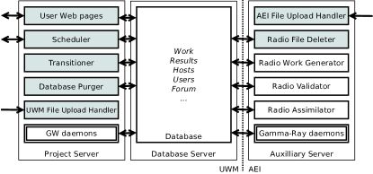
Figure 1.— A schematic of the most important processes running on the Einstein@Home project servers, located in the USA (at UWM) and in Germany (at AEI). They communicate with a single central database, that ensures coordinated operation and ties the parts together. The components in gray boxes are generic to all BOINC projects and come directly from the BOINC software distribution. The components in white boxes are specifically adapted or written for Einstein@Home. The gravitational-wave (GW) and $\gamma$-ray workunit generator, file deleter, validator, assimilator are not listed individually but simply labeled “daemons”. The arrows pointing externally represent network communication with BOINC clients and volunteers. The download servers (which provide astrophysical data to the BOINC clients) are not illustrated.

The programs are coordinated through a single central MySQL database, which runs on a high-end server, and is the “heart” of the project. The most important database tables are the User Table, which has one row for each registered volunteer, the Host Table, which has one row for each host computer that has contacted the Einstein@Home project, the Work Table, which has one row for each Workunit (described later), and the Result Table, which has one row for each separate instance of the Workunit, that is completed, in progress, or not yet assigned to a specific host. (For validation purposes, more than one result is obtained for every workunit, so separate tables are used for work and results.) There are other tables which are less central and not described here, for example the Forum Table contains community message board items posted by project staff or volunteers.

The majority of the other Project Server components are long-running background processes. They typically query the database for a particular condition, take some action if needed, then sleep for some seconds or minutes. For example the Validator checks a database flag to see if there is a workunit with a quorum of completed results. If so, it compares the results as described in Section 4.15 to see if they agree. If they agree, it labels one of these as the “correct” (canonical) result, grants “computing credits” to the volunteers whose hosts did the work, and marks the workunit as completed. If the results do not agree, it sets a flag in the database, which will then be seen by the transitioner, which will in turn generate a new result for that same workunit. Another example is the Workunit Generator, which creates the rows in the work table. Each row contains the name and version of the application program to run, the correct command line arguments and input file name(s), estimates of the required CPU-time and memory size required, and so on.

An additional set of project server components communicates with hosts. The File Upload Handler receives completed results from the BOINC client, through the normal HTTP port 80. This ensures that any host which has Web access can be used to run Einstein@Home. The Scheduler parses the XML scheduler request files from the BOINC client. These typically contain requests for new work, or report completed work that has been uploaded as just described. The Scheduler then queries the database to find new work suitable for the host, or updates the database to mark that a result has been obtained, and sends an XML reply to the host. On Einstein@Home, Scheduler requests typically arrive at the project server at a rate of several Hz.

2.6.3 BOINC Workflow and Validation

As explained above, the fundamental design principle of BOINC is that everything is unreliable, even maliciously so, with the exception of the Project Servers. Thus, when work is sent to hosts, a correct result might be returned, an incorrect result might be returned, a maliciously “falsified” result might be returned, or the host machine and its work might simply vanish, never again contacting the Project Server. In this hostile environment, BOINC achieves reliability through replication and validation.

To implement this, the components shown in Figure 1 operate as a state machine. Initially a workunit is created (formally: a row in the Work Table) by the workunit generator. The transitioner then creates a quorum of “unsent results”. These are rows in the Result Table, not yet assigned to hosts. During its the first year of operation, Einstein@Home used a quorum of three; since then it has used a quorum of two: to be recognized as valid, “matching” results must be returned from hosts owned by at least two different volunteers. The scheduler receives requests from hosts, and eventually assigns the results to suitable host machines owned by different volunteers. The results are then marked with the identity of the host and with a deadline that is typically two weeks in the future.

If the computation for the two results is finished and returned to the server within the deadline, then they are compared by the validator (described in more detail in Section 4.15). If they agree, then one of the results is chosen as the canonical result, both hosts and volunteers are credited, and the workunit is over. If the results do not agree, or if one of the results did not run to completion and generated a non-zero exit code, or if a result is not returned to the server by the deadline, then the transitioner generates another result (again, a row in the Result database table) which is subsequently sent by the scheduler to yet another host owned by yet another user. This process continues, until a quorum of valid results is obtained.

To date, in the Einstein@Home search of the PALFA dataset, approximately 176 million results have been generated and completed.

3. The PALFA Survey

The PALFA Survey (Cordes et al., 2006) was proposed and is managed by the PALFA Consortium, consisting of about 40 researchers (including students) at about 10 institutions around the world. Since 2004, operating at 1.4 GHz, it has been surveying the portion of the sky that is visible to Arecibo (zenith angle less than $20^{\circ}$) within $\pm 5^{\circ}$ from the Galactic plane. To carry out a complete survey will require about $47\,000$ separate pointings of the 7-beam system, or about $330\,000$ separate beams of data.

Within our Galaxy it is estimated that approximately $20\,000$ normal radio pulsars and a similar number of millisecond pulsars (MSPs) beam toward Earth. The PALFA survey, and the High Timing Resolution Universe survey (HTRU-North: Barr 2011; Ng & Barr 2010; HTRU-South: Keith et al. 2010) are the final step before a full census of Galactic radio pulsars is obtained with next-generation telescopes such as the Square Kilometer Array (SKA; Cordes et al., 2004). Taking into account achievable sensitivities and radio scattering limitations, approximately half of these objects are plausibly detectable with SKA (Cordes et al., 2004; Smits et al., 2009). Approximately 1% of these potentially-observable radio pulsars are double neutron-star (DNS) binaries, and about two-thirds of the MSPs are in binaries with white-dwarf companions. About one-quarter of all of these systems are within the portion of the sky visible to the Arecibo telescope. The PALFA survey was initiated to find these pulsars, and to identify the rare systems that give high scientific returns and act as unique physical laboratories.

Radio pulsars continue to provide unique opportunities for testing theories of gravity and probing states of matter otherwise inaccessible to experimental science. Of particular interest are pulsars in short-period orbits with relativistic companions, ultrafast MSPs with periods $P<1.5$ ms that provide important constraints on the nuclear equation of state (Hessels et al., 2006), MSPs with stable spin rates that can be used as detectors of long-period ($\gtrsim$ years) GWs (Kramer et al., 2004), and objects with unusual spin properties, such as those showing discontinuities (“glitches”) and apparent precessional motions, both “free” precession in isolated pulsars (Nelson et al., 1990; Stairs et al., 2000; Jones & Glampedakis, 2011; Jones, 2012) and geodetic precession in binary pulsars (Weisberg et al., 1989; Weisberg & Taylor, 2002; Konacki et al., 2003). Long period pulsars (periods $\gtrsim 2$ s) are of interest for understanding their connection with magnetars (McLaughlin et al., 2003; Ho, 2013). Pulsars with translational speeds (revealed through subsequent astrometry) in excess of 1000 km s^-1 constrain both the core-collapse physics of supernovae (Chatterjee et al., 2005; Nordhaus et al., 2012; Wongwathanarat et al., 2013, e.g.) and the gravitational potential of the Milky Way (Chatterjee et al., 2005, 2009).

There is also a long-term payoff from the totality of pulsar detections, which can be used to map the electron density and its fluctuations, and map the Galactic magnetic field. In the same vein, multi-wavelength analyses (including infrared, optical and high energy observations) of selected objects provide further information on how neutron stars interact with the Interstellar Meduim (ISM), on supernovae-pulsar statistics, and on the relationship of radio pulsars to unidentified sources found in surveys at other wavelengths.

3.1. Importance of, and Expected Numbers of, Pulsars in Short-orbital-period Binaries

Strong-field tests of gravity using pulsars have a notable history. The Hulse-Taylor binary PSR B1913$+$16, a DNS with a 7.75 hr orbital period, loses orbital energy via gravitational radiation precisely as predicted by general relativity (Taylor et al., 1979). Measurements of post-Newtonian orbital effects permit the neutron star masses to be measured to high precision, and provide high-precision tests of the consistency of general relativity (Taylor & Weisberg, 1989). The shorter 2.4 hr orbital period of the double pulsar J0737$-$3039 provides even better tests of general relativity (Kramer & Wex, 2009). There are strong incentives to search for binaries with still shorter orbital periods; such compact systems would provide further stringent tests of general relativity. But short orbital-period systems containing active radio pulsars are rare, so any new discoveries are extremely important.

It is not difficult to estimate the number of short orbital-period DNS in the Galaxy. We only need an estimate for the DNS Galactic merger rate, and a formula for the lifetime of a DNS system as a function of its orbital period $P_{\textrm{orb}}$. Estimating the DNS Galactic merger rate is not easy (Kim et al., 2005; O’Shaughnessy et al., 2005, 2008); current estimates (Abadie et al., 2010) are $R\sim 10^{-4\pm 1}$ yr^-1. The GW inspiral time for a circular system of two 1.4 solar-mass neutron stars starting from orbital period $P_{\textrm{orb}}$ is $\tau=\tau_{0}(P_{\textrm{orb}}/P_{0})^{8/3}$, with $\tau_{0}\approx 7.1\leavevmode\nobreak\ \rm Myr$ and $P_{0}=1\leavevmode\nobreak\ \rm hr$ (Peters & Mathews, 1963; Peters, 1964). Thus the expected period for the most compact DNS in our Galaxy is determined by $R\tau=1$, implying that the shortest-period DNS in our Galaxy should have a period $P=P_{0}(R\tau_{0})^{-3/8}=5\leavevmode\nobreak\ \rm minutes$ (the above range of $R$ values yields shortest expected periods from 2 minutes to 12 minutes). The only assumptions are that the orbital eccentricity is small at the shortest expected orbital period, and that most DNS systems are born with orbital periods short enough that their inspiral time is much less than the Hubble time, 13 Gyr. Both assumptions are reasonable: some discussion of the first may be found in Section 4.5.

To estimate of the number of short orbital-period DNS systems one might expect to find in PALFA data, we also need to know what fraction of these systems beam towards Earth. Equation (15) of Tauris & Manchester (1998) predicts beaming fractions of 30%-40% for pulsars having period less than $\approx 200$ ms; 20% seems a reasonable compromise between short-period pulsars (which tend to have broader beams) and long-period pulsars that have narrower beams.

To be detectable in PALFA data, the pulsars must not only beam toward Earth, they must also lie in the part of the sky visible to PALFA. Simulations of the DNS population show that these systems are concentrated toward the Galactic plane and the Galactic center (Kiel et al., 2010). While Arecibo can see the inner Galaxy, it can not point closer than $30^{\circ}$ to the Galactic center; we estimate that $\approx 25$% of the DNS population falls within the sky area covered by PALFA. Thus, multiplying the beaming and coverage factors, we conclude that $\approx 5$% of all DNS systems should be detectable in PALFA data. This number agrees well with a similar estimate for the detectability of DNS in the PMPS (Osłowski et al., 2011).

If 5% of Galactic DNS systems are detectable in the PALFA survey, the merger rate of this subset is $0.05\leavevmode\nobreak\ R$; setting $0.05\leavevmode\nobreak\ R\tau=1$ increases the expected value of the shortest orbital period by a factor of ${0.05}^{-3/8}\approx 3.1$. Thus we expect there to be a DNS system visible in the PALFA survey with an orbital period of $\approx 16$ minutes (the range of $R$ values given above yields shortest-expected orbital periods ranging from 7 to 37 minutes). Since the probability distribution of intervals between events in a Poisson process is exponential, there is a $1-e^{-1}\approx 63\%$ probability of finding a system with a period shorter than the expected value we have calculated. There is a $1-e^{-2}\approx 86\%$ probability of finding a system with a period shorter than twice this expected value.

One can derive similar ranges by scaling from the observed numbers of longer-period systems. Estimates (Burgay et al., 2003; Osłowski et al., 2011) indicate that the Galaxy may contain as many as $2\,000$ DNS binaries, with periods $<10\leavevmode\nobreak\ \rm hr$, of which $\sim 20$% would beam toward us. Using the period/lifetime scaling relationship above (modulo assumptions about birth orbital periods, whose probability distribution must be convolved with that due to GW emission) there should then be about 50 DNS systems with periods smaller than the 2.4-hr period of the double pulsar J0737-3039, or about 10 that beam toward us. These numbers then suggest that there will be $\approx 1$ object beamed toward Earth with a 1-hr period or less, consistent with our estimate in the previous paragraph. Given the uncertainties, there is a reasonable chance that such a DNS binary can be found in the PALFA survey.

In addition, some neutron-star/white-dwarf binaries will also spiral in from GW emission while the MSP is still active as a radio pulsar (Ergma et al., 1997). Given that these systems are far more numerous than DNS binaries, and that pulsars in neutron-star/white-dwarf binaries are longer-lived MSPs, there should be a sizable number visible in PALFA data with orbital periods less than 1 hr.

Although the prospects are not encouraging, it would be very exciting to discover a radio pulsar in orbit about a black hole. This would likely consist of a normal neutron star with a canonical magnetic field $\sim 10^{12}$ G; the neutron star would probably be “canonical” rather than “recycled” because the more massive black hole progenitor would have formed earlier (O’Shaughnessy et al., 2005, 2008). Unfortunately the relatively short radio-emitting lifetime of canonical pulsars compared to recycled pulsars, along with the expected smaller absolute number of neutron-star/black-hole binaries compared to DNS binaries, suggests that the number of detectable objects in the Galaxy is small.

3.2. Data Acquisition Spectrometers: WAPPS and Mocks

As briefly described in Section 1, data are taken with ALFA: a seven feed-horn, dual-polarization, cryogenically-cooled radio camera operating at 1.4 GHz (Cordes et al., 2006). The polarizations are summed, to produce an radio frequency signal centered on $\sim 1.4$ GHz. This is then fed to fast, broad-band autocorrelation spectrometers. Until 2009 April, the PALFA survey used correlator systems, the Wideband Arecibo Pulsar Processors (WAPPs; Dowd et al., 2000) to compute and record correlation functions every $\Delta t=64\leavevmode\nobreak\ \mu$s. These mix a 100 MHz bandwidth to baseband and calculate the autocorrelation for 256 lags. The correlation functions are recorded to disk as two-byte integers combined with appropriate header information in a custom format. The Einstein@Home analysis used data sets of $2^{22}$ samples, covering 268.435456 s.

The $64\leavevmode\nobreak\ \mu$s sample interval was chosen because many pulsars have small duty cycles $W/P\ll 1$ (where $W$ is the pulse width and $P$ the spin period) yielding $\sim P/W$ harmonics that can be combined into a test statistic (the harmonic sum). The fast sampling retains sensitivity to spin periods as short as $P\sim 1$ ms combined with duty cycles as small as $W/P\sim 1/16$. If it were not for the practical constraints of hardware and data volume, even faster sampling would be desirable.

The complete set of autocorrelation functions for a single 268 s pointing is recorded in 12 files, each $\approx 2$ GB in size. Each set of three files contains the data for two beams. (The last set of three files contain one “phantom” beam of zeros, or a copy of another beam.)

Since 2009 April, PALFA has used broader-band higher-resolution Mock spectrometers that incorporate digital polyphase filter banks. The Mock spectrometers cover a frequency bandwidth of 300 MHz, from 1.175 to 1.475 GHz in 1024 channels, with a sample time of $64\leavevmode\nobreak\ \mu$s and a dynamic range of 16 bits per sample. The operational plan is to cover the entire survey region ($330\,000$ beams) with this higher-resolution system.

The Mock spectrometers acquire data with 16-bit resolution, which is more than we need. To reduce the burden of transfer and storage, data are rescaled to 4-bit resolution at Arecibo Observatory. To help preserve weak pulsar signals in Gaussian-like noise, the rescaling-algorithm clips outliers (typically arising from RFI). For each 1 s chunk of data, the median $\mu$ and rms $\sigma$ are computed for each channel. The data are clipped to the range ($\mu-2.5\sigma,\,\mu+3.5\sigma$), the floor is subtracted, then the data are rescaled to 4 bits. The floor subtraction also flattens the 1 s average bandpass response. The offset and scaling factors (per channel, per chunk) are saved in the data structure, and could be used to approximate the original 16-bit data if desired.

The WAPP data were originally acquired and stored in 16-bit format. In 2011, to reduce the storage volume, it was also reduced to 4-bit format. The expected total data volume from the complete PALFA survey is expected to be about 700 TB.

3.3. Historical Data Acquisition and Processing Rates

In order to understand how Einstein@Home can be used for analysis of PALFA data, we need to compare the current and historical data acquisition rates to the Einstein@Home data processing rate. On average, PALFA has been granted about 265 h of telescope time per year. About 12% of the time is used for follow-up confirmation and initial timing of newly-discovered pulsars. Overhead (telescope slewing, calibration) consumes another 12%. So about 200 hr of actual survey data are obtained each year.

Calendar	Inner	Total	Beams	Beams
Year	Time	Time	acquired	analyzed
2004	69 h	108 h	$15\,149$ P
2005	278 h	365 h	$25\,320$ W
2006	250 h	360 h	$28\,649$ W
2007	72 h	143 h	$11\,275$ W
2008	182 h	184 h	$6\,640$ W
2009	180 h	186 h	$6\,832$ M	$6\,130$ W
2010	249 h	275 h	$10\,066$ M	$60\,032$ W
2011	175 h	434 h	$24\,710$ M	$7\,430$ M
2012	83 h	334 h	$14\,126$ M	$27\,861$ M
			$15\,149$ P
Totals	$1\,538$ h	$2\,389$ h	$71\,844$ W	$66\,162$ W
			$55\,734$ M	$35\,291$ M

Table 1Annual observation times and data collection volumes for the PALFA blind search survey at the Arecibo Telescope, and for Einstein@Home data processing. “Inner time” denotes observations towards the inner Galaxy; “total time” also includes pointings in the opposite direction, towards the outer Galaxy. “W” and “M” indicate WAPP or Mock spectrometer data; “P” indicates pre-survey WAPP data, not analyzed by Einstein@Home.

The annual telescope time (inner Galaxy and total) and data collection volumes are shown in Table 1 from the beginning of the PALFA survey in 2004. The numbers are lower in years when there were no (commensural) observations antipodal to the inner Galaxy. Painting work in 2007 and platform repairs in 2010 also reduced observing time. The fourth column lists the number of beams of blind-search survey data acquired in that year, and the spectrometer used. If everything works correctly, seven beams are acquired in parallel for each telescope pointing. The last column shows the number of beams processed by the Einstein@Home data analysis pipeline. The overall processing speed of the Einstein@Home data analysis pipeline is discussed in Section 4.13. As shown in Table 1, as of the end of 2012, after nine years of operation, the PALFA survey had acquired $142\,767$ beams of blind-search survey data.

The accounting of beams of WAPP survey data searched by Einstein@Home is as follows. The $15\,149$ beams of 2004 WAPP data were taken in a pre-survey (p1944) mode. These were not searched by Einstein@Home because they had a shorter time-baseline than the p2030 data that followed, and the sky pointings were repeated in the p2030 pointings. Of the original $71\,844$ beams of WAPP p2030 data, 995 beams were not transferred to AEI, and $70\,849$ beams were transferred to AEI. Of these, $2\,102$ beams were not sent for pre-processing because the corresponding data file counts were incorrect; $68\,747$ beams were sent to pre-processing. Of these, $1\,591$ beams could not be pre-processed because of data corruption or scaling or similar issues; $67\,156$ beams were sent to Einstein@Home hosts for processing. Of these, $994$ beams had enough errors during run-time that the corresponding workunits errored-out or were canceled. Hence $66\,162$ beams of WAPP data were fully-searched by Einstein@Home.

As of 2013 January 1, Einstein@Home had analyzed a total of $101\,453$ beams ($66\,162$ WAPP and $35\,291$ Mock); it is currently processing about 160 beams of Mock data per day (see Section 4.13 for details). Provided that sufficient telescope time is granted, the survey will continue and will eventually be extended to higher Galactic latitudes. We expect the extension to higher latitudes to increase the yield of MSPs, since they are distributed more widely and their detection is inhibited by multi-path propagation (interstellar scattering) that is stronger at low Galactic latitudes.

3.4. Data Storage and Movement

Data are recorded to RAID storage systems at the Arecibo Observatory. Disks containing the data are then shipped to the Cornell Center for Advanced Computing (CAC), where the raw data are archived on RAID storage systems for use by the PALFA Collaboration. For the Einstein@Home search, the data are transmitted over the Internet using GridFTP from CAC to the AEI in Hannover, Germany. At AEI, they are stored on a Hierarchical Storage Management system.

4. The Einstein@Home Radio Pulsar Search

The following is a detailed description of how the E@H radio pulsar search works.

4.1. Preparation of the PALFA Data

4.1.1 WAPP Data

Before being sent to host machines, data are prepared in a series of pre-processing steps. The first step is Fourier transformation of the autocorrelation functions. This produces dynamic power spectra with 256 frequency channels of $390\,625$ Hz spanning 100 MHz. The channelization allows compensation for the dispersive propagation of any pulses from celestial sources.

At AEI, preprocessing is performed separately for each group of three files containing the autocorrelation functions for two beams. A script preprocess.sh calls the Cornell/ALFA program alphasplit to split the files into two sets of three files, each containing data from a single beam. For each beam, the script then calls filterbank from the SigProc package. This reads the three files containing data for that beam. The output is a small text header, and a 4 GB file containing $2^{22}$ time samples of a dynamic power spectra with $256$ channels; power is represented as a 4-byte float. The header is combined with the data using addheader; the resulting files (one per beam) are the input to the Einstein@Home Workunit Generator.

4.1.2 Mock Data

The first step in the preparation of the Mock data combines two overlapping sub-band files into a single file with no redundant data, covering a 300 MHz bandwidth with 960 channels. The Mock data used for the Einstein@Home pipeline consist of two 4-bit psrfits files for each beam. Each file covers a bandwidth of 172.0625 MHz in 512 channels, one file contains data from a band centered on 1450.168 MHz, the other from a band centered on 1300.168 MHz. The sub-band files are $\approx 1.2$ GB in size, the combined psrfits file is $\approx 1.9$ GB.

A RFI mask is then computed using presto (Ransom et al., 2002, 2003) software tools. In addition, strong periodic RFI is identified and added into a beam-specific “zap list”. The RFI mask is used in the generation of the work units (see next section), while the zap list is sent to the Einstein@Home hosts with all work units of a given beam.

4.2. Workunit Generation

The workunit generator has been described in connection with Figure 1. It is an “on demand” BOINC server process that prepares data files and “processing descriptions” for the computational work done on Einstein@Home hosts. The workunit generator reads as input one data file per beam, prepared as described in Section 4.1. As output it generates data files (628 per WAPP beam, 3808 per Mock beam) which are later downloaded by Einstein@Home hosts for analysis. Each of these files contains one de-dispersed time series, for a different value of the dispersion measure (DM). The workunit generator also creates one row in the database Work Table for each beam and for each DM value; these contain information such as the command-line arguments for the search application.

To generate workunits from the WAPP input data files, the data for each beam are de-dispersed with 628 different DM values, and then down-sampled by a factor of two to 128 $\mu$s. For the WAPP data, a single de-dispersed time series has $2^{21}$ time samples with 32 bits per sample, yielding 8.3 MB per time series.

DM range	$\Delta\text{DM}$	number of trial values
(pc cm-3)	(pc cm-3)
$0\;-\;212.4$	$0.6$	$355$
$212.4\;-\;348.4$	$1$	$136$
$348.4\;-\;432.4$	$2$	$42$
$432.4\;-\;1002.4$	$6$	$95$
$0\;-\;213.6$	$0.1$	$2136$
$213.6\;-\;441.6$	$0.3$	$760$
$441.6\;-\;789.6$	$0.5$	$696$
$789.6\;-\;1005.6$	$1.0$	$216$

Table 2 Set of DM trial values used in the Einstein@Home search of the PALFA WAPP (upper half) and Mock (lower half) data.

The discrete DM values are piecewise linear with four distinct slopes as shown in Table 2; they range from 0 to a maximum of 1002.4 pc cm^-3. Since there are (mostly inner-Galaxy) pulsars with even larger DM values, we may increase this maximum in future searches: compact H II regions can create significant additional dispersion. The spacing at small DM is set by the requirement that the “smearing” over the entire observed radio bandwidth arising from the discreteness of DM is less than one sample time. At larger DMs, the smearing over a single frequency channel becomes the dominant effect. Also, the increasing electron density along the line of sight leads to multi-path scattering and pulse broadening (Lorimer & Kramer, 2004), which creates an effective time-smearing larger than the sampling time. Work by Bhat et al. (2004) derived a heuristic relationship between this pulse broadening and DM; the pulse broadening increases slightly faster than quadratically with DM. The increasing DM spacing shown in Table 2 is obtained by requiring that the time-smearing arising from DM discreteness is smaller than the effective pulse broadening from single-channel smearing and multi-path scattering. Further details may be found in Section 2.4.2 and 3.7.2 of Knispel (2011).

For the generation of workunits from the Mock data, 3808 different trial DM values up to 1005.6 pc cm^-3 are used, determined with the DDplan.py tool from presto and shown in Table 2. The de-dispersion is done with other tools from the same software suite, using the previously mentioned RFI masks to replace broad- and narrowband RFI bursts by constant values. Mock data are not down-sampled, so there are $2^{22}$ samples per de-dispersed time series. We initially used a dynamic range of 8 bits per sample but halved it to 4 bits early in 2012 to reduce Internet bandwidth. The de-dispersed time series generated from Mock data currently have file sizes of 2.1 MB.

The workunits cannot all be generated at once. This would overload the Einstein@Home database server with huge number of rows in the Work and Result Tables; the resulting time-series data files would also overflow the Einstein@Home download storage servers. So the Workunit Generator is automatically run “on demand” when the amount of unsent work drops below a low-water mark; it is automatically stopped when the amount of work reaches a high-water mark. In this way, the project typically maintains a pool of tens of thousands of unassigned results.

To reduce the load on the Einstein@Home database server and increase the run-time per host, up to eight de-dispersed time series are bundled into a single work unit, as discussed in Section 4.13.

4.3. Signal Model and Detection Statistic

In searching for possible signals hidden in noise, a model for the signals is required. Here, we describe the model used for the signal from a constant-spin-rate neutron star in a circular orbit with a companion star.

The phase model $\Phi$ for the fundamental mode of the signal emitted by a uniformly rotating pulsar in a circular orbit of radius $a$ can be written in the form

$$\Phi\left(t;\mathbf{\Lambda}\right)=2\pi f\left(t+\frac{a\sin\left(i\right)}{c}\sin\left(\Omega_{\text{orb}}t+\psi\right)\right)+\Phi_{0},$$ (1)

where $f$ is the apparent spin frequency of the pulsar, $t$ is time at the detector, and $a\sin\left(i\right)$ is the length of the pulsar orbit with inclination angle $i$ projected onto the line of sight. The orbital angular velocity $\Omega_{\text{orb}}$ is related to the orbital period $P_{\text{orb}}$ via $\Omega_{\text{orb}}=2\pi/P_{\text{orb}}$. The angle $\psi$ denotes the initial orbital phase and $\Phi_{0}$ is the initial value of the signal phase. $\mathbf{\Lambda}$ denotes the ensemble of signal phase parameters $\mathbf{\Lambda}=\{f,a\sin\left(i\right),\Omega_{\text{orb}},\psi,\Phi_{0}\}$.

The time-domain radio intensity signal is a sum of instrumental and environmental noise ${\mathcal{N}}(t)$ and a pulsar signal formed from harmonics of this fundamental mode

$$s\left(t;\mathbf{\Lambda}\right)\equiv{\mathcal{N}}(t)+\sum_{n=1}^{\infty}s_{n}\left(t;\mathbf{\Lambda}\right)$$ (2)

where the intensities of each harmonic are given by

$$s_{n}\left(t;\mathbf{\Lambda}\right)\equiv\Re\bigl{[}\mathcal{A}_{n}\exp\left[in\Phi\left(t;\mathbf{\Lambda}\right)\right]\bigr{]}.$$ (3)

The $\mathcal{A}_{n}$ are the complex amplitudes of the different signal harmonics; their values are determined by (or define) the profile of the observed de-dispersed radio pulse.

We define a detection statistic $\mathcal{P}_{n}$ for the $n$th harmonic through correlation of the radio intensity with the $n$th normalized signal template $\exp\left[-in\Phi\left(t;\mathbf{\Lambda}\right)\right]$ for the putative signal. This detection statistic is optimal in the Neyman-Pearson sense: thresholding on it minimizes the false-dismissal probability at fixed false-alarm probability (Allen et al., 2002). It can also be obtained by maximizing a signal-to-noise ratio (S/N), under the assumption that the initial phase $\Phi_{0}$ is unknown and has a uniform probability distribution; see Appendix B of (Allen, 2005).

In a search for pulsars, the parameters $\mathbf{\Lambda}$ are not known, and so that precise point in parameter space might not be searched. However the signal will still appear at a nearby point ${\mathbf{\Lambda}}^{\prime}$, for which

$$\mathcal{P}_{n}\left(\mathbf{\Lambda},\mathbf{\Lambda}^{\prime}\right)=\left|\frac{1}{T}\int_{0}^{T}\!\!\!\!\operatorname{d}\!t\;s\left(t;\mathbf{\Lambda}\right)\exp\left[-in\Phi\left(t;\mathbf{\Lambda}^{\prime}\right)\right]\right|^{2}.$$ (4)

Note that $\mathcal{P}_{n}$ is independent of $\Phi_{0}$ and $\Phi_{0}^{\prime}$ because of the maximization described above. Therefore from here onward we use $\mathbf{\Lambda}=\{f,a\sin\left(i\right),\Omega_{\text{orb}},\psi\}$ to denote a point in the four-dimensional search parameter-space.

If there is no pulsar signal, or it is very weak, the expected value of this detection statistic is proportional to the power spectrum of the instrumental noise in the neighborhood of frequency $nf$. On the other hand, if the pulsar signal is strong (in comparison with the noise, so $\mathcal{N}(t)$ can be neglected), then the expected value is

$$\langle\mathcal{P}_{n}\left(\mathbf{\Lambda},\mathbf{\Lambda}^{\prime}\right)\rangle\approx$$ (5)

$$\left|\frac{\mathcal{A}_{n}}{2}\right|^{2}\left|\frac{1}{T}\int_{0}^{T}\!\!\!\!\operatorname{d}\!t\;\exp\left[in\left(\Phi\left(t;\mathbf{\Lambda}\right)-\Phi\left(t;\mathbf{\Lambda}^{\prime}\right)\right)\right]\right|^{2}.$$

This assumes that the observation time $T$ is much longer than the pulsar period: $fT\gg 1$.

If the instrumental/environmental noise $\mathcal{N}$ is Gaussian , then the detection statistic $\mathcal{P}_{n}$ is described by a non-central $\chi^{2}$ distribution with 2 degrees of freedom, one coming from each of the real and imaginary parts of the integrand in Equation (4). The strength of the pulsar signal determines the non-centrality parameter: in the absence of a pulsar signal the non-centrality parameter is zero.

The detection statistics $\mathcal{P}_{n}$ for different values of $n$ may be combined to form other detection statistics. If the pulse profile were known in advance, a particular weighted sum would be optimal. Since in practice for blind searches this is not the case, we need to make some arbitrary choices about what statistics to construct, and how many such statistics to construct.

To design statistics, we simply assume that radio pulsars have profiles that resemble a Dirac delta-function, truncated to some finite number of harmonics. A delta-function has equal weights in all the amplitudes ($|\mathcal{A}_{n}|$ independent of $n$) so we have chosen to use statistics that equally weight the $\mathcal{P}_{n}$ up to some maximum harmonic. This choice also makes it simple to characterize the false alarm probability associated with the resulting statistic.

Thus we define five detection statistics $S_{0},\dots,S_{4}$ by incoherently summing the values of $\mathcal{P}_{n}$

$$S_{L}\equiv\sum_{n=1}^{2^{L}}\mathcal{P}_{n}.$$ (6)

The statistic $S_{0}$ is proportional to the power in the fundamental harmonic of the pulsar rotation period; the statistic $S_{4}$ equally weights the power in the first 16 harmonics. In the noise-only case the probability distribution of $S_{L}$ is

$$p\left(S_{L}\right)\operatorname{d}\!S_{L}=\chi^{2}_{2N}\left(2S_{L}\right)\operatorname{d}\!\left(2S_{L}\right),$$ (7)

which is a chi-square distribution with $2N=2^{L+1}$ degrees of freedom.

The false-alarm probability $p_{\text{FA}}$ is the probability that $S_{L}$ exceeds some threshold value $S_{L}^{*}$ in the absence of a signal. This is given by the area under the tail of the probability distribution $p_{\text{FA}}=Q_{2N}\left(2S_{L}^{*}\right)$, where

$$Q_{2N}\left(x\right)=\Gamma\left(x;2N\right)=\frac{1}{\Gamma\left(2N\right)}\int_{x}^{\infty}\!\!\operatorname{d}\!y\,y^{2N-1}e^{-y}$$ (8)

is the complement of the cumulative $\chi^{2}$ distribution function: the incomplete upper Gamma function. This may be easily computed by means of analytical or numerical approximations.

The detection statistic is unlikely to assume large values in random Gaussian noise; large values are indications that a pulsar signal may be present (or that RFI is providing a significant background of non-Gaussian noise). We define the significance of such a candidate as

$$\mathcal{S}\left(S_{L}\right)\equiv-\log_{10}\left(p_{\text{FA}}\right).$$ (9)

A candidate with significance of (say) 30 has a probability of $10^{-30}$ of appearing in Gaussian random noise.

4.4. Template Banks

In a search for unknown new pulsars, as explained before Equation (4), one evaluates the detection statistics $S_{L}({\mathbf{\Lambda}}^{\prime})$ at many points in the parameter space $\mathbf{\Lambda}=\{f,a\sin\left(i\right),\Omega_{\text{orb}},\psi\}$. In order to enhance the statistical likelihood of detection (to maximize the S/N) one would like to evaluate this quantity at precisely the correct point in parameter space ${\mathbf{\Lambda}}^{\prime}={\mathbf{\Lambda}}$ where the pulsar is located. But this is impossible, since the pulsar parameters ${\mathbf{\Lambda}}$ are not known before discovery!

In a practical search, $S_{L}({\mathbf{\Lambda}}^{\prime})$ is calculated for many different values of ${\mathbf{\Lambda}}^{\prime}$. These “trial values” of the unknown pulsar parameters must be spaced “closely enough” that not too much S/N is lost from the mismatch between ${\mathbf{\Lambda}}$ and ${\mathbf{\Lambda}}^{\prime}$. However if they are spaced too closely, precious computer cycles are wasted, because $S_{L}({\mathbf{\Lambda}})$ and $S_{L}({\mathbf{\Lambda}}^{\prime})$ are correlated if $\Delta{\mathbf{\Lambda}}={\mathbf{\Lambda}}-{\mathbf{\Lambda}}^{\prime}$ is small.

The set of points in the parameter space ${\mathbf{\Lambda}}$ where the detection statistic is evaluated is called a template grid or template bank. An optimal grid will maximize the probability of detection at fixed computing cost; in general it will not be a simple regular Cartesian lattice with uniform spacings along each axis. Within the GW detection community, substantial research work has shown how to construct optimal or near-optimal template grids (Owen, 1996; Owen & Sathyaprakash, 1999; Harry et al., 2009; Messenger et al., 2009, ; H. Fehrmann & H. Pletsch 2013, in preparation); we make use of those ideas and methods here.

The most important tool for setting up a template bank is the metric (Owen, 1996) on the search parameter space. To simplify matters, consider only the detection statistic $S_{0}=\mathcal{P}_{0}$ for the fundamental harmonic of the pulsar. The metric measures the loss of the expected strong-signal detection statistic which arises if the parameters of the search point ${\mathbf{\Lambda}}^{\prime}$ are mismatched from those of the putative signal ${\mathbf{\Lambda}}$. It follows immediately from Equation (5) that this loss is described by a quadratic form in $\Delta{\mathbf{\Lambda}}$, since the second modulus-squared term on the right-hand-side (rhs) is maximized (at unity) if the signal and search parameters match exactly ($\Delta{\mathbf{\Lambda}}=0$). Thus the fractional loss of detection statistic (called the mismatch $m$) must be quadratic in $\Delta{\mathbf{\Lambda}}$ as one moves away from this maximum:

$$m\left(\mathbf{\Lambda},\mathbf{\Lambda}^{\prime}\right)=1-\frac{\langle\mathcal{P}_{0}\left(\mathbf{\Lambda},\mathbf{\Lambda}^{\prime}\right)\rangle}{\langle\mathcal{P}_{0}\left(\mathbf{\Lambda},\mathbf{\Lambda}\right)\rangle}=g_{ab}\Delta\Lambda^{a}\Delta\Lambda^{b}+O(\Delta{\mathbf{\Lambda}}^{3}).$$ (10)

Here the indices $a$ and $b$ label the four parameter-space coordinates $f$, $a\sin\left(i\right)$, $\Omega_{\text{orb}}$, and $\psi$, and we adopt the Einstein summation convention where repeated indices (in this case $a$ and $b$) are summed. We assume the strong signal limit, so $\langle\mathcal{P}_{o}\rangle$ is defined as in Equation (5).

It is straightforward to show that $g_{ab}$ is a positive-definite symmetric quadratic form: a metric of signature $(+,+,+,+)$. The components of the metric can be computed directly from the phase model Equation (1). A short calculation yields

$$g_{ab}=\langle\partial_{a}\Phi\partial_{b}\Phi\rangle_{T}-\langle\partial_{a}\Phi\rangle_{T}\langle\partial_{b}\Phi\rangle_{T},$$ (11)

where the angle brackets denote a time-average $\langle\mathcal{G}\rangle_{T}\equiv\frac{1}{T}\int_{0}^{T}\mathcal{G}\left(t\right)\,\operatorname{d}\!t$ and $\partial_{a}$ denotes the partial derivative with respect to the $a$’th component of $\mathbf{\Lambda}$.

If the mismatch is small (positive, but much less than unity) then the surface of constant mismatch is a ellipsoid in parameter space. The problem of efficient template bank construction is to cover the desired part of parameter space with the smallest possible number of these ellipsoids for a given nominal mismatch $m_{0}$. For a general (non-constant, as here) metric this template bank is not regular or uniform.

The quadratic approximation in Equation (10) is inaccurate for typical Einstein@Home mismatches ($m_{0}=0.2$ or $0.3$). For these values, the region of parameter-space covered by a template is banana-shaped rather than ellipsoidal; see Figure 3. Thus, in creating template banks, mismatches are computed using the exact definition Equation (10) rather than the metric approximation. Nevertheless, the metric is still useful, as described below.

4.5. Parameter space searched by Einstein@Home

In order to carry out a search the parameter space must be covered with a suitable template bank. Thus, one must decide what region of parameter space to cover: what range of pulsar spin frequencies, orbital periods, etc. should be searched? With unlimited computing resources, one could search the entire physical parameter space. In practice, Einstein@Home has finite computing power, so we can only search some part of parameter space. Just as an intelligent gambler needs to decide whether to play blackjack or poker, we need to decide where (in parameter space) to invest our precious compute cycles. What parameter-space regions are most likely to yield a scientific pay-off?

The region to search is astrophysically motivated and targets the Einstein@Home search to the most likely range of putative pulsar orbital parameters and spin frequencies. We constrain the search parameter space by setting a probabilistic limit on projected orbital radii, and by an upper limit on spin frequencies.

As described in Section 2.4, standard acceleration searches lose sensitivity where $P_{\text{orb}}\lesssim 10T$. For the PALFA data, this is $P_{\text{orb}}\lesssim 45$ minutes. Since other search pipelines within the PALFA collaboration use standard accelerations searches, the Einstein@Home search was set up to complement these efforts. Thus, the longest orbital period in the Einstein@Home search is chosen to be $45$ minutes (plus one template for an isolated system).

The lower limit on $P_{\text{orb}}$ is determined by the available computing power: as we show below, the computing cost grows rapidly as the minimum orbital period decreases. We choose $P_{\text{orb}}\gtrsim 11$ minutes, significantly increasing sensitivity to pulsars in compact binary systems.

Even for these short orbital periods, for the purposes of detection, we can neglect relativistic corrections $\mathcal{O}((v/c)^{2})$ to the phase model (1), because they correspond to less than a single cycle of phase error. In the worst case, the value of $(v/c)^{2}\approx 4\times 10^{-6}$ for $P_{\text{orb}}=660$ s and $a\sin(i)=0.2$ lt-s. Thus, the additional phase accumulated over $T=268$ s for a signal at $f=400$ Hz is $\Delta\Phi\approx fT(v/c)^{2}\approx 0.4<1$ cycles. This corresponds to an acceptable worst-case 19% loss in detection statistic.

Our search, described by the phase model Equation (1), assumes circular orbits. However as described in Section 4.8 the search is still sensitive to pulsars in orbits with eccentricities $e\leq 0.1$. Both theoretical arguments and extrapolation from known pulsars in binaries suggests that by the time they evolve to the short periods that are the new feature of the Einstein@Home search, their orbits will be circularized by the emission of gravitational radiation.

We now review the arguments and expectations regarding orbital eccentricity $e$. The majority of known pulsar/white-dwarf binaries have very small orbital eccentricities ($e\lesssim\text{few}\times 10^{-4}$) (Lorimer, 2008). Known DNS systems typically have larger orbital eccentricities, but their orbital periods are much longer than the target values for Einstein@Home. These systems will evolve by the emission of GWs, which over time circularizes the orbits (Peters & Mathews, 1963; Peters, 1964). If the known DNS systems from Lorimer (2008) are evolved until their orbital periods drop to $11$ minutes, they are well described by a circular phase model: the evolved eccentricities $e_{11}$ at an $11\,$minute orbital period are very small compared to the present-day values. This is not surprising: binaries formed with short periods and large $e_{11}$ would decay rapidly through emission of gravitational radiation. With the exception of PSR B1913$+$16 ($e_{11}=0.0302$) and PSR B2127$+$11C ($e_{11}=0.0416$), we find that $e_{11}\lesssim 0.005$ for all known DNS systems. Highly evolved pulsars in such systems are therefore detectable by the Einstein@Home search as show in Section 4.8.

Mass transfer in X-ray binaries also circularizes the orbits of radio pulsars in compact binaries. As Archibald et al. (2009) have shown, X-ray binaries can become visible as binary radio pulsars after the accretion stops and radio waves from the pulsar can escape the system and reach Earth. The orbits of these systems are quickly circularized during the phase of mass transfer (Stairs, 2004). For example, the X-ray binary with the shortest known orbital period (about 11 minutes) is X$1820-303$ (Smale et al., 1987). If the mass transfer stopped and a radio pulsar emerged, it would have an almost perfectly circular $11\,$minute orbit. Such objects would probably not be found by an acceleration search, but might be detected by Einstein@Home.

The constraints on the projected orbital radius $a\sin(i)$ are determined by the expected ranges of pulsar and companion masses. We allow the maximum allowed value of $a\sin(i)$ to depend on pulsar and companion masses and on the orbital period. From Kepler’s laws we find

$$a\sin(i)\leq\alpha F\left(m_{\text{c,max}},m_{\text{p,min}}\right)\Omega_{\text{orb}}^{-\frac{2}{3}},$$

where $m_{\text{c,max}}$ is the maximum companion mass and $m_{\text{p,min}}$ is the minimum pulsar mass. The function

$$F\left(m_{\text{c,max}},m_{\text{p,min}}\right)=\frac{G^{\frac{1}{3}}m_{\text{c,max}}}{c(m_{\text{p,min}}+m_{\text{c,max}})^{\frac{2}{3}}}$$ (12)

is a mass-dependent scaling factor, where $G$ is the gravitational constant. The parameter $0\leq\alpha\leq 1$ bounds the orbital inclination angles: for given masses $m_{\text{p,min}}$ and $m_{\text{c,max}}$, and given $\alpha$, this condition defines an upper limit on the projected orbital radii as a function of the orbital angular velocity. For the Einstein@Home search we selected $\alpha=0.5$, $m_{\text{p,min}}=1.2$ M_⊙ and $m_{\text{c,max}}=1.6$ M_⊙.

We can use Equation (4.5) to calculate the fraction $p$ of the total possible solid angle $4\pi$ steradians in which the normal vector to the orbital plane may lie. The distribution of possible orbital inclination angles is uniform in $\cos\left(i\right)$ and thus the fraction $p$ of systems with inclination angles between $0$ and $i$ is $p=1-\cos\left(i\right)=1-\sqrt{1-\sin(i)^{2}}$. For arbitrary pulsar ($m_{\text{p}}$) and companion ($m_{\text{c}}$) masses, we may write the orbital radius as $a=F\left(m_{\text{c}},m_{\text{p}}\right)\Omega_{\text{orb}}^{-\frac{2}{3}}$. Inserting this in the left-hand-side of Equation (4.5) yields $\sin(i)\leq\alpha F\left(m_{\text{c,max}},m_{\text{p,min}}\right)/F\left(m_{\text{c}},m_{\text{p}}\right)$. From this, the fraction $p$ follows

$$p=1-\sqrt{1-\alpha^{2}\left(\frac{F\left(m_{\text{c,max}},m_{\text{p,min}}\right)}{F\left(m_{\text{c}},m_{\text{p}}\right)}\right)^{2}}.$$ (13)

This quantity, the fraction of orbital inclination vectors covered by the Einstein@Home search parameter space, is shown in Figure 2.

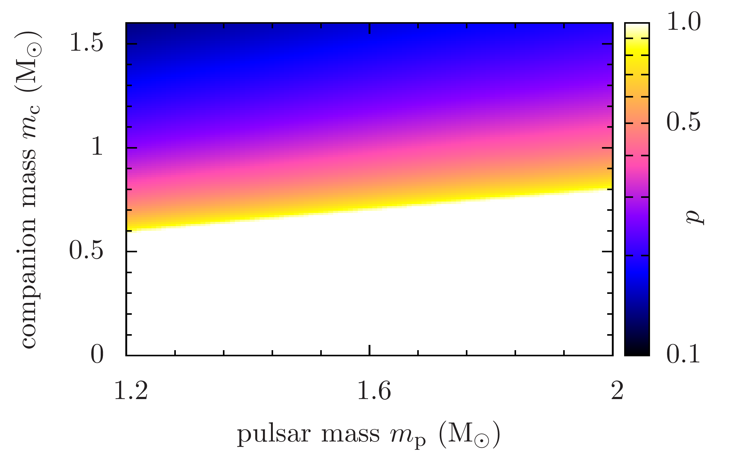
Figure 2.— The fraction $p$ of total solid angle covered by the Einstein@Home search parameter space, Equation (13). The horizontal axis shows the pulsar mass and the vertical axis the companion mass. All systems in the white region are detectable for any inclination angle, elsewhere only a fraction $p$ has favorable orbital inclinations.

The Einstein@Home search parameter space is also constrained in maximum spin frequency $f<f_{\text{max}}$. As explained in Section 4.6, the number of orbital templates grows with $f_{\text{max}}^{3}$. So one must strike a compromise, choosing a frequency for which Einstein@Home can detect a large fraction of millisecond (and slower) pulsars, while not exceeding the available computing power. The search grid is designed to recover frequency components up to $f_{\text{max}}=400$ Hz.

The constraints above define a wedge of orbital parameter space, shown in Figure 3.

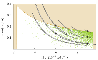
Figure 3.— The white region is the “design wedge” of orbital parameter space searched by Einstein@Home, as described in Section 4.5. The vertical axis is the projected orbital radius, the horizontal axis is the orbital angular velocity, and the initial orbital phase $\psi\in[0,2\pi)$ dimension is suppressed. The dots are the orbital template locations, constructed as described in Section 4.6. For a few orbital templates (located at the black crosses) the region of mismatch $m<0.3$ at fixed $\psi$ for $f=f_{\text{max}}$ is shown in gray. As discussed in Section 4.4 the template coverage regions are banana-shaped, not ellipsoidal.

The shorter PALFA data sets spanning $T=134$ s have different parameter space constraints. The orbital period range was halved, to $\SI{5.5}{minutes}\leq P_{\text{orb}}\leq\SI{22.5}{minutes}$, which also sped up the overall data analysis. We re-invested this gain into searching for higher spin frequencies $f\leq 660$ Hz. The constraint on the projected radius was left as in Equation (4.5).

In the part of the PALFA survey using the Mock spectrometers, there also are some observations covering $T=536$ s. For the Einstein@Home pipeline we only used the first half of these observations.

4.6. Template Bank Construction for Einstein@Home

For the Einstein@Home search, we have chosen to construct a template bank which is completely regular and uniform in the frequency dimension. Thus, our template bank is the direct Cartesian product of a uniformly-spaced grid in frequency with a three-dimensional orbital template bank in the remaining parameters ${\mathbf{\Lambda}}_{\text{orb}}=\{a\sin\left(i\right),\Omega_{\text{orb}},\psi\}$. Having uniform frequency spacing simplifies matters and allows the use of Fast Fourier Transforms (FFTs) in the frequency-domain; FFTs are computationally very efficient if the frequency points are uniformly-spaced.

In this paper template bank refers to the four-dimensional grid, and orbital template bank to the three-dimensional grid. To construct the orbital template bank, a three-dimensional “orbital” metric is obtained by projecting the metric $g_{ab}$ onto the sub-space $f=$constant. A detailed calculation of the four-dimensional metric $g_{ab}$ and the three-dimensional projected metric may be found in Knispel (2011).

If a metric is constant or approximately constant, then lattice-based methods (Owen & Sathyaprakash, 1999) can be employed to generate templates covering the parameter space. However the metric here is not even approximately constant, and alternative methods are needed. Two simple and efficient methods are random template banks (Messenger et al., 2009), and stochastic template banks (Harry et al., 2009).

For a random template bank, template locations are chosen at random with a coordinate density proportional to the volume element: the square-root of the determinant of the metric. The expected number of templates can be calculated from the proper volume of the search parameter space and the chosen coverage $\eta$ and nominal mismatch $m_{0}$ (Messenger et al., 2009).

Stochastic template banks are formed in the same way, but then in a second step, superfluous templates (those closer than the nominal mismatch) are removed.

For both random and stochastic template banks, the goal is to cover most, but not all, of the parameter space; the coverage $\eta\leq 1.0$ describes the fraction of parameter space which lies within the nominal mismatch of one of the template grid points.

As described, Einstein@Home template banks are a Cartesian product of a one-dimensional uniform frequency grid with a three-dimensional orbital template bank. This affects the construction of the orbital template bank in three important ways.

First, the orbital template bank must be created for the highest frequency used in the search. This is because the same orbital template bank is used at all frequencies. Thus its spacing (mismatch) must be the finest needed at any frequency. The spacing is finest at the highest frequency $f_{\text{max}}$, because the expected detection statistic Equation (5) depends upon the difference in phase, which varies most rapidly at the highest frequency. The total number of orbital templates required at a given mismatch and coverage grows like $f_{\text{max}}^{3}$ because the grid coordinate spacings are proportional to $1/f_{\text{max}}$ in each of the three dimensions.

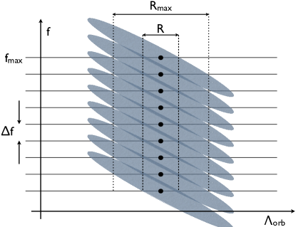
Figure 4.— A schematic of template coverage in the parameter space with coordinates $\mathbf{\Lambda}$. The vertical axis is frequency $f$, the horizontal axis denotes the orbital parameters $\mathbf{\Lambda}_{\text{obs}}$, and the horizontal lines denote frequency bins, separated by $\Delta f\approx 1\,$mHz and extending up to $f_{\text{max}}=400\,$Hz. The dark dots show template locations; the ellipse denotes the coverage region (mismatch $m=0.2$) of one orbital template. Because the four-dimensional grid is a Cartesian product, the orbital template is reproduced at each frequency bin, separated by $\Delta f$. At fixed frequency a single template covers a small region $R$ of orbital parameters. However the “cookie cutter” copies of the templates cover a much larger region $R_{\text{max}}$ of orbital parameter space, obtained by minimizing the mismatch over frequency and orbital parameters. The four-dimensional mismatch $m=0.3$ is allowed to be somewhat larger, hence $R_{\text{max}}$ includes a small amount of parameter-space outside the orbital templates. This illustration is only schematic because the coverage region of a template is not elliptical in shape (see Figure 3) and can extend over more than a hundred frequency bins.

Second, this affects how mismatches are computed between two orbital templates, in creating a stochastic bank, as illustrated in Figure 4. Because the orbital templates are reproduced at every frequency bin, a given orbital template covers a larger region of the orbital parameter space than that defined by its overlap with the surface $f=f_{\text{max}}$. The orbital and frequency parameters are degenerate: one can recover most of the detection statistic at the incorrect orbital parameter value, provided that the frequency value is also mismatched. If the frequency and orbital parameters are denoted $\mathbf{\Lambda}=\{f,\mathbf{\Lambda}_{\text{orb}}\}$, then the mismatch between two orbital templates is

$$m({\mathbf{\Lambda}}_{\text{orb}},{\mathbf{\Lambda}}_{\text{orb}}^{\prime})\equiv\min_{f^{\prime}}m(\{f_{\text{max}},{\mathbf{\Lambda}}_{\text{orb}}\},\{f^{\prime},{\mathbf{\Lambda}}_{\text{orb}}^{\prime}\}).$$ (14)

In practice, the minimum does not occur for $f^{\prime}$ widely separated from $f_{\text{max}}$, so one does not need to search a very large range. Typically for $f_{\text{max}}=400\,$Hz the range needed is less than $\pm 150\,$mHz.

Third, the mismatch in the four-dimensional parameter space may be larger than that in the three-dimensional space; in this work the corresponding values are $0.3$ and $0.2$.

As previously described, Einstein@Home uses five distinct detection statistics $S_{0},\dots,S_{4}$, which weight contributions up to the sixteenth harmonic of the pulsar spin frequency. However we use the same template bank for all of these. The template banks are designed using only the detection statistic $\mathcal{P}_{0}=S_{0}$. Since that statistic only measures the power in the fundamental mode of the pulse profile, it corresponds to building a search optimized for sinusoidal pulse profiles. Thus in constructing and testing template banks, we only use noise-free simulated pulsar signals whose intensity profile varies sinusoidally at the spin frequency.

Because it was quick and easy, Einstein@Home initially used a random orbital template bank with $22\,161$ templates. However after approximately ten months of operation, this was replaced by a stochastic orbital template bank containing $6\,661$ templates. This required an investment of computer time and human effort, but was justified because the orbital template bank is used in the analysis of every de-dispersed time series.

4.7. Parallel Construction of Stochastic Template Banks

It required about $200\,$khr of dedicated computer cluster time to produce a stochastic bank which was about one-quarter the size of the initial random template bank. This reduced the total Einstein@Home computing time by a factor of two, saving hundreds of millions of CPU hours. The parallelized construction algorithm for metric-assisted stochastic template placement is described in more detail in Section 3.5 of Knispel (2011); we summarize it here.

Begin by fixing the desired mismatch $m_{0}$ (here $m_{0}=0.2$). To describe the algorithm, it is useful to define operations on template banks. As before, a template bank (denoted $A$ or $B$) is a set of distinct points in parameter space (denoted $a$ or $b$). A template bank $A$ is called non-overlapping if for all distinct points $a,a^{\prime}\in A$ one has $m(a,a^{\prime})>m_{0}$.

The algorithm works by combining pairs of template banks to produce new ones. For the description, it is helpful to define a merge and prune operation which we denote $P$. This operation takes as arguments (or inputs) two non-overlapping template banks, and returns (or produces) a single non-overlapping template bank:

$$P(A,B)=A\cup\left\{b\in B\;|\;m(a,b)>m_{0}\text{\ for\ all\ }a\in A\right\}.$$ (15)

It is easy to see that if $A$ and $B$ are both non-overlapping, then $P(A,B)$ is also non-overlapping. It is also easy to parallelize into independent parts.

The algorithm begins with $2^{p}$ non-overlapping template banks, and proceeds through $p$ reduction steps, each of which halves the number of template banks. Each step takes as its input $2^{j}$ non-overlapping template banks, and produces as its output a set of $2^{j-1}$ non-overlapping template banks. To carry out a reduction step, the template banks are grouped into $2^{j-1}$ pairs $A,B$, and each pair is replaced by $P(A,B)$. These have increasingly higher coverage at fixed nominal mismatch. This procedure continues until a single bank remains, which is the final output of the procedure.

The algorithm can be trivially parallelized, because a single merge and prune operation can be trivially parallelized. If the non-overlapping template bank $B$ is partitioned into $n$ disjoint pieces $B=\bigcup_{i=1}^{n}B_{i}$, then

$$P(A,B)=\bigcup_{i=1}^{n}P(A,B_{i}).$$ (16)

This also holds if the partition is not disjoint, but is computationally less efficient.

In practice, the template bank $B$ is partitioned into roughly equal-sized pieces so that the merge and prune operations take similar time. The number $n$ of partition elements is selected so that the compute time required by the merge and prune operations (proportional to the product of the number of templates in each argument: $|A||B_{i}|$) is independent of the reduction level.

For the Einstein@Home search, we construct a template bank using $\mathcal{O}(1000)$ CPU-cores of the Atlas computer cluster (Aulbert & Fehrmann, 2009). The number of partitions $n$ is chosen so that the merge and prune operations $P(A,B_{i})$ take about one hour.

The initial input is $2^{p}=1024$ non-overlapping template banks. These are produced as random template banks, each containing $M=100$ templates, corresponding to $\eta\approx 0.01$ at mismatch $m_{0}=0.2$. Then all $M(M-1)/2$ inter-template mismatches (14) are computed and templates closer than mismatch $m_{0}$ are removed.

We compute the coverage of the final template bank with Monte-Carlo simulation (or integration). We begin with a large number of simulated noise-free signals at random points $\mathbf{\Lambda}$ in the parameter space. As discussed earlier, these have pulse profiles containing only the fundamental mode $\mathcal{A}_{i}=0\text{\ for\ }i>1$: the detection statistic is $\mathcal{P}_{0}=S_{0}$. For each signal, the mismatch $m$ is computed for all templates, and the minimum is recorded. The coverage $\eta$ is the fraction of simulated signals with mismatches $m<m_{0}$.

The coverage can also be monitored in the prune and merge operations: when 99% coverage has been achieved, $|P(A,B)|$ contains 1% of the points from $|B|$. If sufficient coverage has been achieved the reduction procedure can be terminated “early” (before the reduction index $j=0$). In this case, one of the $2^{j}$ remaining template banks is arbitrarily chosen as the output.

4.8. Template Bank Verification

We constructed a template bank with $\eta=90$% coverage and nominal mismatch $m_{0}=0.3$ as described above. For the PALFA data spanning $T=268\,$s it covers the region of parameter space described in Section 4.5 with $6\,661$ orbital templates. For data spanning $T=134$ s, the bank (which now goes to shorter orbital periods and higher frequencies) contains $7\,113$ orbital templates. In both cases a single template with $a\sin(i)=0$ was added by hand to facilitate the detection of isolated pulsars by the Einstein@Home pipeline. The obtained stochastic orbital template bank is shown in Figure 3.

Monte-Carlo integration (as described in the previous section) was used to verify that the template banks have the specified coverage and nominal mismatch. This was done using $20\,000$ noise-free signals at $f=f_{\text{max}}$ with random orbital parameters and a sinusoidal pulse profile as previously discussed. The resulting mismatch distribution (minimum over all templates) is shown in Figure 5. It demonstrates that the template bank has the desired coverage $\eta=0.9$ at nominal mismatch $m_{0}=0.3$. We note that the median mismatch $m_{0.5}=0.17$ is significantly smaller than the nominal mismatch $m_{0}$.

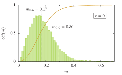
Figure 5.— Test of the Einstein@Home template bank for pulsars in circular orbits with a $T=268\,$s data span. The bars show a histogram of the mismatch distribution for $20\,000$ noise-free signals from simulated pulsars in random circular orbits. The curve shows the cumulative distribution function (CDF) of the mismatch. The median $m_{0.5}$ and the 90%-quantile of the mismatch distribution $m_{0.9}$ have been highlighted. The template bank covers 90% of the parameter space with mismatch $m<0.3$.

We used the same method to test if pulsars in elliptical orbits could be detected by the Einstein@Home pipeline. These signals lie outside our parameter space, which includes only circular orbits. Thus it was unclear how well pulsars in eccentric orbits could be detected by Einstein@Home. We again created $20\,000$ simulated signals at $f=f_{\text{max}}$ with random orbital parameters, but with non-zero orbital eccentricity $e$. Separate tests were done, with eccentricities $e=10^{-4},10^{-3},10^{-2},0.025,0.05$, and $0.1$. The longitude of the periastron was fixed at $\omega=0$ in all runs. As before, the mismatch was minimized over all templates in the bank.

For $e\leq 0.025$, there was no significant change in the mismatch distribution: the median and the 90%-quantile were similar to those obtained for circular orbits. Thus the Einstein@Home search can detect pulsars in orbits with $e\leq 0.025$ without significant sensitivity losses.

For $e=0.05$ and $e=0.1$, as shown in Figure 6, the simulations show clear deviations from the mismatch distribution for circular orbits. The distribution shifts to higher mismatches, reaching e.g. $m_{0.9}=0.48$ for $e=0.1$. In this case, for $10\%$ of the target signals, about half of the detection statistic (squared S/N) is lost: detection is still possible, but the search is less sensitive.

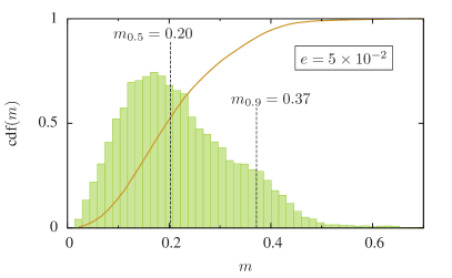
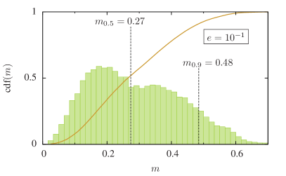
Figure 6.— Test of the Einstein@Home template bank for simulated pulsars in eccentric orbits. The left panel shows the results for $e=0.05$, and the right panel those for $e=0.1$, respectively. The bars show histograms of the mismatch distribution obtained from $20\,000$ simulated noise-free signals. The curve shows the CDF of the mismatch. The median $m_{0.5}$ and the 90%-quantile of the mismatch distribution $m_{0.9}$ are highlighted. For eccentricities of 0.001 and 0.025, there is no significant loss of sensitivity compared with the circular orbit tests.

4.9. Client Search Code

The client search code is the part of the Einstein@Home radio pulsar search pipeline which runs on the volunteers’ hosts and does the bulk of the computing work. Its input is de-dispersed time-series radio intensity data as described in Section 4.2. The client search code computes the detection statistics $S_{0},\dots,S_{4}$ at each template grid point in parameter space, and then returns back to the Einstein@Home server a list of “top candidates”: the points in parameter space where the detection statistic was largest.

The client search code is distributed under the GPL 2.0 license and is publicly available from Einstein@Home, as are binary executables optimized for the complete range of supported OSs and CPU and GPU types. Further details of these optimizations are given in Sections 4.12 and  4.14.

Below, we give a detailed description of how the client search code operates. It carries out five main steps:

I. The time-series data are uncompressed and type-converted.

II. The data are shifted into the frequency domain and whitened, frequency bins affected by RFI are “zapped”, and the data are shifted back into the time domain.

III. For each orbital template, this new time series is re-sampled in the time-domain to remove the effects of the orbital motion.

IV. The detection statistics $S_{0},\dots,S_{4}$ are computed in the frequency-domain using an FFT, searched over frequency for the largest values, and five lists of top candidates are maintained.

V. When the iteration over orbital templates is complete, the lists of top candidates are merged and the most significant candidates are returned to the Einstein@Home server.

These steps are schematically illustrated in Figure 7 and described in detail below.

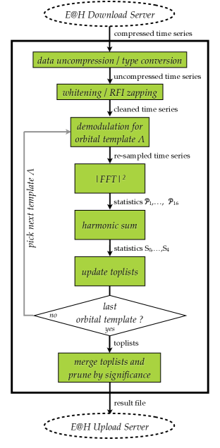
Figure 7.— Data analysis on the Einstein@Home hosts, as described in Section 4.9. The client search code (rectangular box) receives a de-dispersed time series as input from the Einstein@Home download server. The data are searched with a large number of orbital models, then a list of the most statistically-significant candidates is returned to the Einstein@Home upload server.

4.9.1 (I) Data Uncompression / Type Conversion

The uncompression and type conversion is done immediately after the client search code receives its input: one of the 628 WAPP (3808 Mock) different de-dispersed time-series data sets described in Section 4.2. In producing these, the original 16-bit or 4-bit instrumental data are converted to floating-point format for de-dispersion on the Einstein@Home server. To reduce the network bandwidth required to transmit it to the host, the time-series is down-sampled to 4-bits (and if a significant compression factor can be achieved, compressed with gzip). The first action of the client search code is to uncompress the data if required, and then convert it back into IEEE-754 single-precision floating point representation. A factor from the data file header is used to set the overall scale. This is only needed to avoid dynamic-range problems, and is irrelevant in what follows.

4.9.2 (II) Whitening / RFI Zapping

The next stage of client processing is to whiten the time domain data. Whitening is necessary because instrumental noise and RFI can result in a very colored data spectrum. If the detection statistic were computed from this colored data, it would be impossible to compare the statistical significance $\mathcal{S}$ for templates at different frequencies. In addition, the detection statistics $S_{1},\dots,S_{4}$ would be dominated by the “noisiest” frequency band which appeared in the harmonic sum, and their statistical distribution would no longer be described by the $\chi^{2}$ distribution of Equation (7), which would make it impossible to compare the statistical significance of different candidates.

To whiten the time-domain data (time-span $T$) they are first padded with $2T$ of zeros to produce a time-series of length $3T$. The data (which have had the mean removed) are then converted into the frequency domain using an FFT. The individual frequency bins have a frequency width $\Delta f\approx 1\,$mHz; their contents are complex Fourier amplitudes. The modulus-squared of each amplitude (a periodigram) is computed bin by bin, then replaced with a running median value $\mathcal{M}$ using a sliding boxcar window of width $\pm 500$ bins (covering $\pm 0.62\,$Hz). Finally, the data are whitened by multiplying the amplitude in each bin by $\sqrt{\ln\left(2\right)/\mathcal{M}}$. (For Gaussian data this normalization yields real and imaginary parts that are zero-mean unit-variance Gaussians.) The first and last 500 bins are not whitened and are excluded from further analysis.

We use the term “zapping” to describe the process of replacing data in frequency bins that are contaminated with RFI with random Gaussian noise. Zapping is needed because RFI introduces regular (periodic) variations into the radio intensity that can mimic pulsar signals and would dominate the candidate lists if not removed. In Section 4.10 we describe the “toplist clustering” technique that is used to create a list of top candidates. For most beams, these candidates are not dominated by RFI, although for certain beams the most significant candidates are from RFI.

The frequency bands to be zapped were selected from a database of candidates generated by the Cornell pulsar search pipeline (J. Deneva & J. Cordes 2013, private communication). The basic idea is that if an apparently periodic signal appears in many different sky positions (beams) at different observation times, it can not be a radio pulsar, but must be due to RFI.

The Cornell candidate database contained $2\,030\,604$ candidates up to frequency 7.8125kHz and over the complete range of trial DMs up to 1000pc cm^-3. In the database, $654\,468$ of these candidates had been flagged as arising from RFI. These candidates were binned in frequency bins of width $\approx 3.7\,$mHz. Frequency bins containing more than 200 candidates were then broadened by a fractional amount of $1.05\times 10^{-4}$ to account for Doppler shift in frequency arising from Earth’s orbital motion. Overlapping frequency bands were then merged to obtain a set of non-overlapping bands, and frequency intervals of $\pm 0.25\,$Hz around the first three harmonics of the power-line frequency (60, 120, and 180 Hz) were added. For the Einstein@Home search, the relevant part of the zap list is transmitted to the host along with the search executable.

The zap list is a two-column table of lower and upper frequency values, and extends up to the Nyquist frequency 3.90625kHz of the down-sampled data. The same zap list is used for all beams: it contains a total of 233 bands covering 72.383Hz, which represents 1.85% of the total bandwidth of 3.9kHz. Figure 8 shows the total frequency bandwidth zapped as a function of the frequency. Note that some recent work has demonstrated that RFI at Arecibo is highly time-dependent, so using a fixed zap list is not optimal. In future Einstein@Home searches it may be beneficial to instead use dynamic beam-dependent zap lists.

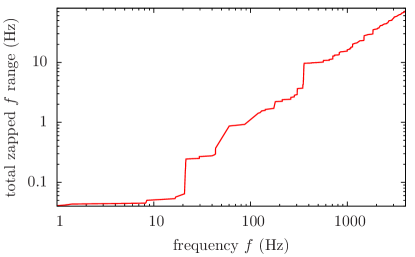
Figure 8.— The total frequency bandwidth zapped by the fixed zap list used in the Einstein@Home search as a function of the frequency $f$. Below $f=100$ Hz about $1$ Hz (1% of the data) is zapped.

The Einstein@Home search client receives this zap list and replaces the amplitudes of the corresponding frequency bins in the whitened Fourier spectrum with computer-random-number-generated zero-mean Gaussian noise whose real and imaginary parts have unit variance. Then the whitened and zapped Fourier amplitudes are inverse-FFT’d to shift the data back to the time domain. After the inverse FFT the time series is cut back to its initial length $T$ by removing the previously padded bins at the end. This data conditioning is done only once per de-dispersed time series when the science code is started. However if the code is restarted from a checkpoint, the data conditioning is repeated, since it takes just a fraction of a second; the whitened and zapped time series is not stored on the Einstein@Home hosts.

Whitening is done before and not after zapping, because typical RFI corrupts at most a handful of bins and so does not significantly bias the median estimator used for the whitening normalization.

4.9.3 (III) Orbital Demodulation

The client search code now begins to step through the orbital templates one-by-one. For each orbital template with orbital parameters $\mathbf{\Lambda}$, the detection statistics $S_{L}$ of Equation (6) are computed on the full frequency grid with spacing $\Delta f=1/3T$.

The detection statistics can be efficiently computed in the frequency domain. To do this, the time-series is first re-sampled so that instead of being indexed by uniform steps of time $t$ at the telescope, it is indexed by uniform steps of time $t^{\prime}$ at the binary system’s barycenter. This demodulation is done by replacing the $k$’th sample of the time series at time $t=k\Delta t$ by the sample closest (nearest neighbor) to time $t^{\prime}(t)$. The time coordinate $t^{\prime}$ at the binary system’s barycenter is defined by the condition $\Phi(t,\mathbf{\Lambda})\equiv 2\pi ft^{\prime}$. The definition of the pulsar spin phase Equation (1) then implies

$$t^{\prime}=t+\frac{a\sin\left(i\right)}{c}\sin\left(\Omega_{\text{orb}}t+\psi\right).$$ (17)

Offsets in time $t^{\prime}(t=0)\neq 0$ are dropped. They correspond to constant phase offsets $\Phi_{0}$, on which the detection statistic in Equation (4) do not depend.

This transformation means that the phase which appears in the exponential of the detection statistic Equation (4) becomes $\exp(-2\pi inft^{\prime})$. Then Equation (4) simply becomes a Fourier transform: the detection statistic $\mathcal{P}_{n}$ is the squared-modulus of the Fourier amplitude of the re-sampled time series in the $n$th frequency bin.

Before the re-sampled time series is FFT’d to compute the detection statistics, it is padded with its mean value in the same way as described earlier: to a total time interval of $3T$. This lessens the reduction of the detection statistic for putative pulsar signals with frequencies that do not fall exactly at the center of a Fourier frequency bin; the maximum loss is 8.8% (Knispel, 2011).

4.9.4 (IV) Detection Statistic Computation

The client search code internally maintains five different candidate lists (called “toplists”) corresponding to the detection statistics $S_{0}$ through $S_{4}$. Here “candidate” denotes the point in parameter space as well as the value of $S_{i}$. The $i$th toplist includes the 100 candidates with the largest values of $S_{i}$ having distinct values of fundamental frequency $f$. The toplists are initialized with null entries ($S_{i}=0$) and then updated as follows.

After the time domain data have been demodulated for an orbital template and FFTd, five arrays are created, indexed by frequency $f$, which contain $S_{0}$ through $S_{4}$. Note that these statistics are obtained by combining values of $\mathcal{P}$ for harmonically-related frequency bins. This “harmonic summing” can be quite compute intensive, in part because it requires striding over widely separated parts of the frequency-domain arrays, summing elements. For computational efficiency, the number of required summations are minimized by re-using the $S_{L}$ with smaller $L$ to compute those with larger $L$ (Lorimer & Kramer, 2004).

The array containing the detection statistic $S_{i}$ is then stepped through, element by element. If the statistic $S_{i}(f)$ is less than the smallest statistic currently on the $i$th toplist, then the next element is considered. Otherwise, the toplist is searched to see if it contains a candidate at the same fundamental frequency $f$. If not, the toplist candidate with the smallest detection statistic is replaced with the new, higher-statistic candidate. If so, then the candidate at the same frequency is replaced with the new candidate if and only if the new candidate has a larger value of the detection statistic than the existing candidate. This procedure ensures that the 100 entries on each toplist are for 100 distinct frequencies.

The comparison process required to insert new candidates in the toplist can be quite compute-intensive. To speed it up, the comparison is only carried out for values of the detection statistic that lie above a predefined threshold. The threshold is data-independent: it is the largest statistic value expected in Gaussian noise for the relevant number of “independent trials” (roughly speaking, this is the number of orbital templates $\times$ the number of frequency bins). Further details may be found in Section 4.10

4.9.5 (V) Result Files

When the loop over orbital templates is finished, the search code computes the statistical significance Equation (9) of the 500 candidates stored in the five toplists. These are then winnowed further: the 100 candidates with the largest statistical significance are selected, sorted into canonical order, and returned to the Einstein@Home server in a single result file. The remaining 400 candidates are dropped.

Each de-dispersed time series generates one fixed-format ASCII text result file. Five lines contain identifiers for the volunteer and the computer that did the computation, the date that the computation was completed, and similar information. The remaining 100 lines are for the most significant 100 candidates winnowed from the toplists.

Each candidate line contains seven white-space-separated values: the spin frequency $f$ in Hertz, the orbital period $P_{\text{orb}}$ in seconds, the projected orbital radius $a\sin(i)$ in light-seconds, the initial orbital phase $\psi$ in radians, the detection statistic $S_{L}$, the statistical significance $\mathcal{S}$ defined by Equation (9), and the number of harmonics $2^{L}$.

4.10. Thresholding and Candidate Selection

As discussed above, candidates are only checked against toplist entries if their statistics $\mathcal{P}_{n}$ exceed certain thresholds. These thresholds are computed from a false-alarm probability, provided as command-line parameter to the search code.

The false-alarm probability for each orbital template in any de-dispersed time series is set to $p_{0}=0.08$. For 6661 orbitals templates and in pure Gaussian noise data, we expect $6661\times 0.08\approx 530$ candidates to exceed this threshold after all orbital templates have been searched. Thus, the search code should always return $\gg 100$ candidates for each $\mathcal{P}_{n}$, after searching the complete template bank, and fully populate all five toplists.

For easy thresholding during runtime, the global false-alarm threshold $p$ is converted into a single-FFT-bin false-alarm threshold $p_{\text{single}}$ and thresholds on the detection statistics $\mathcal{P}_{n}^{*}$. The probability of not having a false-alarm in $N_{f}$ frequency bins in random Gaussian noise is $1-p=(1-p_{\text{single}})^{N_{f}}$. From this, we find $p_{\text{single}}=1-(1-p)^{1/N_{f}}$. The detection statistic threshold $\mathcal{P}_{n}^{*}$, is determined indirectly by $p_{\text{single}}=Q_{2N}(2\mathcal{P}_{n}^{*})$, where $Q$ is the incomplete upper gamma function as in Equation (8).

We compared these expectations, based on Gaussian noise, with results from real data, and were able to verify that the Einstein@Home search is not dominated by non-Gaussian noise. The returned candidates in a single de-dispersed time series typically have $\mathcal{S}\gtrsim 8.5$, unless strong pulsar or RFI signals are present. For most beams this is not the case. The number of total trials per de-dispersed time series (neglecting parameter correlations in the detection statistic) is the product of the number of frequency bins and the number of orbital templates $N_{\text{tot}}=N_{f}\times N_{\text{templ}}=3\times 2^{21}\times 6661\approx 4\times 10^{10}$. Assuming that the number of candidates exceeding a particular significance threshold follows binomial statistics, one expects of order $N_{\text{tot}}\times 10^{-8.5}\approx 133$ candidates with $\mathcal{S}\gtrsim 8.2$ from noise alone. Indeed, the search code always reports $\gtrsim$100 candidates, validating the assumption above.

As described, each beam is analyzed with 628 different DM values for WAPP data and 3808 different DM values for Mock data, respectively. For each DM value, the 100 top candidates are returned. So the search procedure always returns $62\,800$ “candidates” or $380\,800$ “candidates” per beam, respectively, regardless of whether RFI is present or absent in the beam. Moreover, the 100 candidates for each DM value are at distinct frequencies. This makes it harder for RFI to dominate the candidates for a given beam.

There is a consensus among radio astronomers that RFI has become more severe in the past decade, probably due to the proliferation of wireless devices such as cellphones and WiFi. Nevertheless, the procedures we have described are reasonably effective in mitigating the effects of this RFI. The Einstein@Home search is not dominated by non-Gaussian noise, in the sense that a typical beam returns statistic values in the expected ranges for Gaussian noise. Of course there are beams which contain strong RFI or strong pulsars for which this is not the case.

If one looks across the entire search (not beam-by-beam) the top 1% of candidates are not consistent with Gaussian noise: these arise from pulsars or RFI. However if one looks further down the list, the distribution of statistic values are reasonably consistent with Gaussian noise. In fact the situation is similar for the Pulsar Exploration and Search Toolkit (PRESTO) processing pipeline, which is also used to process PALFA data. In that pipeline, for each beam, the 200 strongest candidates are followed-up (folded and refined). For beams that are strongly affected by RFI, most or all of these candidates are not consistent with Gaussian noise. However for the majority of beams, the bulk of candidates are consistent with Gaussian noise.

4.11. Client Search Code Checkpointing

The search execution on the host may stop for many reasons. For example the volunteer might turn off the computer, or the BOINC client might stop execution because it appears that the volunteer is busy using the computer for other purposes.

As described in Section 2.6.1 the client search code checkpoints on a regular basis, by default once per minute. This checkpointing saves the internal state of the search, and permits it to be efficiently restarted with very little computing time lost. The checkpointing is done by sorting and saving the toplist files, and then saving a counter which records the last orbital template that was completed.

When the search is started (or restarted) it carries out the whitening and zapping steps on the input data, and then checks if a valid checkpoint file exists. If not, the search begins execution at the first orbital template as previously described. However if a valid checkpoint file is found, then the toplists are initialized from the stored values, and the loop over orbital templates begins following the orbital template index recorded in the checkpoint file.

4.12. CPU Implementation of the Search Algorithm

The search algorithm is implemented in the C programming language. Mathematical functions are provided by the standard C math library with special functions from the GNU Scientific Library (Galassi et al., 2009) and FFT routines from the Fastest Fourier Transform in the West (FFTW; Frigo & Johnson, 2005; Johnson & Frigo, 2008) library. The search code is then wrapped into the BOINC framework (Anderson et al., 2006) as described earlier. The implementation is single-threaded, i.e., hosts simultaneously execute one instance on each CPU core that BOINC allocates to the search.

To produce executable binaries, the Linux applications are compiled using standard GNU tools. The applications for Mac OS X are built using the Mac OS X 10.4 SDK build environment. For Windows, the applications are cross-compiled on Linux machines using the MinGW tools. The underlying compiler in all three cases is the GNU C Compiler; this permits identical optimizations and execution ordering on all platforms.

4.13. Einstein@Home Processing Speed / Throughput

The speed with which Einstein@Home can process one beam of PALFA data is determined by the amount of computing time required for a single workunit and the number of workunits per observed beam. These have varied over the years as the processing code was made more efficient; the number of participating volunteers has also varied.

Individual workunits should not take too long to run on a host: volunteers become discouraged if the results of their processing do not quickly lead to successful results and visible computing credits. The workunits also should not be too short, or the Einstein@Home database gets too large to operate efficiently, and the overhead of uploads, downloads, and sending new workunits to hosts becomes excessive. In general our goal has been to have workunit run-times of between one hour and one day. As the application code became faster, we achieved this by bundling multiple single workunits into larger ones: the runtime has remained between one hour and one day for the majority of the hosts, the lower end populated by the GPUs.

The first implementation of the Einstein@Home search ran from 2009 March to 2010 February and processed on average $\approx 25$ WAPP beams each day. After that, two major code improvements increased the processing speed by a factor of $\sim 6$, and between 2010 February and 2010 August, Einstein@Home processed $\approx 160$ WAPP beams per day. The first GPU version of the search code increased the processing rate to more than $300$ beams per day between 2010 September and 2010 December.

The Einstein@Home search of the Mock spectrometer data started in 2011 July and processed on average $\approx 50$ beams per day until 2012 September. After that date, the processing rate gradually increased over a period of three months and has been running at around $160$ beams per day since the end of 2012. As of 2013 February, the majority of the Mock data (see Table 1) has been analyzed, and the data processing backlog is less than two months.

4.14. GPU Implementation of the Search Algorithm

As previously described, Einstein@Home also takes advantage of the GPUs available on a substantial fraction of host machines, providing applications for NVIDIA GPUs which support CUDA version 3.2 or higher, and for AMD/ATI GPUs which support OpenCL version 1.1 or higher. CUDA and OpenCL are programming models, API interfaces, and support libraries which enable GPUs to be used for scientific computation.

The supported GPUs typically execute double-precision floating point operations very slowly compared to single-precision operations, or do not support them at all. So the CPU codes were designed so that all floating-point operations can be performed in single precision. Tests with simulated pulsar signals were performed to ensure that this does not degrade the sensitivity of the search.

The code was also designed to have a reasonably small memory “footprint”, particularly because of limits imposed by consumer-grade graphics cards. The GPU version requires less than 250 MB of GPU memory, which substantially enlarges the set of GPU cards on which the code can run.

The overall structure of the GPU code is similar to that of the CPU version (see Figure 7), with the most compute-intensive analysis offloaded to the GPU. These are the time-series re-sampling to remove the effects of orbital motion via demodulation, the FFT and power spectrum computations, and the harmonic-summing to obtain the $S_{L}$ from the $\mathcal{P}_{i}$. For NVIDIA GPUs, the CUDA 3.2 programming framework was used to embed calls to CUDA-C code (kernels) executing on the GPU. On AMD/ATI GPUs, the OpenCL programming framework was used for the same purpose.

To maximize GPU utilization, the GPU implementation of the time-series re-sampling is split into five CUDA kernels to maximize thread parallelization. To avoid the overhead of memory transfers to the host CPU, intermediate output is kept in GPU memory as much as possible. The time-offsets $t-t^{\prime}$ needed for re-sampling are computed in parallel, using a lookup table and interpolation to avoid costly sine/cosine operations. An identical lookup table is pre-computed for both CPU and GPU hosts to help ensure that their results cross-validate later in the processing pipeline (see Section 4.9). We use intrinsic functions to avoid generating fused multiply-add instructions that could introduce rounding errors which would also hamper cross-validation. The length of the modulated time series is computed in a separate kernel, and the re-sampling itself is done by yet another kernel, using the time-offsets and the time-series length computed in the previously. Each time-series sample is computed in parallel by a separate GPU thread. A parallel sum-reduction algorithm is then used to compute the mean of the re-sampled time-series, and a final CUDA kernel implements the mean-padding of the re-sampled time-series.

To perform FFTs efficiently on NVIDIA GPUs, the NVIDIA cufft 3.2 library is used. The cufft library has an FFTW compatibility mode, which simplified development and integration with the CPU code. A custom CUDA kernel is used to compute the power spectrum in parallel from the FFT output. Intermediate as well as the final output (for the next step) is again kept in GPU memory.

The GPU implementation of harmonic summing differs from the CPU version: the GPU version re-orders the computations so that hundreds of processing cores on the GPU can independently perform calculations in parallel. Memory caching is needed, because of the low locality and irregular access strides associated with summing the different harmonics of $f$. Caching is done in texture memory; without it the memory access pattern of the individual threads would be very inefficient. Write accesses have been eliminated, except for those associated with the (comparatively rare) signals that might make it onto the candidate toplist, i.e. detection statistics exceeding the false-alarm threshold and the weakest toplist signal.

GPU versions of the host applications are provided for Linux, Windows, and Mac OS X operating systems. The Windows version is cross-compiled under Linux for the same reason as described in Section 4.12: to improve cross-platform result validation. This also allows for a tighter integration in the automated build system of Einstein@Home, but adds complexity because cross-compilation requires the use of the lower-level CUDA driver API instead of the higher-level CUDA runtime API.

The OpenCL implementation differs somewhat from the CUDA one. The FFT library is derived from software developed by Apple. As provided, the Apple library can only do complex-to-complex FFTs of arrays whose length is a power-of-two ($2^{n}$); we extended it to efficiently do real-to-complex transforms of length $3\times 2^{n}$, as required by the search code. It was also modified to eliminate calls that approximate trigonometric functions with different accuracy on different GPUs. This reduces the numerical difference between different GPU models, making the results more hardware-independent and simplifying result cross-validation.

OpenCL is a vendor-independent framework and the OpenCL application also runs on NVIDIA graphics cards that support OpenCL 1.1. Somewhat surprisingly, we found better numerical agreement between the OpenCL application running on ATI/AMD GPUs and the CUDA application running on NVIDIA cards, than between the (same!) OpenCL application running on both ATI/AMD and NVIDIA GPUs.

Compute	CPU	% of	CUDA	% of	OpenCL	% of
operation	time	time	time	time	time	time
Uncompress	$<1$ s	$<1\%$	$<1$ s	$<1$ %	$<1$ s	$<1$ %
Whiten	1 s	$<1$ %	1  s	$<1$ %	1  s	$<1$ %
Demodulate	898 s	13 %	20  s	14  %	123  s	41  %
$\lvert FFT\rvert^{2}$	4022 s	59 %	48  s	32  %	59  s	20  %
Harmonic sum	1888 s	28 %	68  s	45  %	107  s	35  %
Update toplists	12 s	$<1$ %	12  s	8  %	12  s	4  %
Merge toplists	$<1$ s	$<1$ %	$<1$ s	$<1$  %	$<1$ s	$<1$ %
Totals	6822 s	100 %	150 s	100 %	299 s	100 %

Table 3 Comparison of run-times for the CPU (using only one core) and GPU versions of the client search application, processing a single de-dispersed time-series through a template bank containing 6662 orbital templates. The different rows show the execution time spent in the different functional blocks of Figure 7. The absolute run-times vary considerably for different combinations of CPU and GPU models; we measured it for typical consumer-grade hardware. The CPU is an Intel Core 2 Q8200 (2.33GHz), the CUDA GPU is a NVIDIA GTX 560 Ti and the OpenCL GPU is an AMD Radeon HD 7970 (all running on unloaded Linux systems).

The GPU version of the search application evolved considerably over time, by incrementally porting more steps of the main loop to code executing on the GPU. The first GPU version of the search application only implemented the FFT step on the GPU, and was limited to a speed-up of between 2 and 3 compared to the CPU version, because on the CPU version the FFT step consumes almost two-thirds of the total CPU run time. The next important step was to port the re-sampling code to the GPU. This gave an overall speed-up of about 4 compared to the CPU version, and left the harmonic-summing step dominating the run time. When the harmonic summing step was also ported to the GPU, the overall speed-up factor reached 50 (and even higher on some CPU and GPU combinations). Table 3 shows typical run time examples for the current GPU and CPU version of the client search application and the relative fraction of time spent in each processing step.

Running one instance of the application, a typical high-end NVIDIA GPU (for example the GTX 560) achieves up to 85% utilization. Provided that the GPU has sufficient memory, BOINC can run two or three instances in parallel. This saturates the GPU, achieving more than 98% utilization!

4.15. Validation

As described earlier, any result file uploaded to the Einstein@Home servers must be validated because it could be partially or completely incorrect, and/or corrupted. Validation is done on the Einstein@Home server, by comparing the result file to another result file for the same workunit, generated on another host. An automatic validator compares results and rejects those that appear to be corrupted and/or inconsistent with other results.

The validation process is not trivial; it cannot be based on a simple binary comparison of the two result files, because the use of different floating-point libraries, compiler instructions, and hardware can lead to numerical differences in the results. Thus, results from two different hosts might both be correct, but not binary identical. So the comparison process must allow for numerical differences at a level which is typically of the order of 1 part in $10^{5}$.

For Einstein@Home, the validation process operates in two steps. The first step checks a single result file for syntax and internal consistency. The second step compares two (or if necessary, more than two) results which have passed the first step against one another. Most incorrect or invalid results are detected in the first step.

In the first “syntax and consistency” step, a result file is checked to see if it has the fixed seven-column output format with 100 lines described near the end of Section 4.9. For each line, the seven fields are individually checked to confirm that they are valid numbers and lie in pre-defined ranges. The overall ordering of lines within the file is also checked to confirm that they are ordered by decreasing significance. If any of these checks fails, then the result is marked invalid, and another copy of the corresponding workunit is generated on the Einstein@Home server sent to a different volunteer’s computer. Slightly less than 1% of results fail to validate at this stage.

In the second step, two or more result files that have passed the first step are pairwise-checked for mutual consistency. The validator tries to match each line from one result file to a line in the other. Two lines “match” when the individual values for DM, $f$, the orbital parameters, the $S_{L}$, and $\mathcal{S}$ agree within less than a fractional error of $10^{-5}$. The number of harmonics $2^{L}$ must match exactly.

The last lines in the result files are typically near the noise threshold and because of differences in floating-point accuracy and rounding on different hosts, they may not correspond to the same candidates. Thus the validator permits unmatched lines in the result files if (within fractional error $10^{-5}$) the corresponding candidate might not have appeared in the most significant 100 results in the other result file.

If two results both pass the “syntax and consistency” step, but are found to be inconsistent, another instance of the work is generated and sent to a different client machine. The process of generating further instances of the results is repeated until a consistent set are found, containing two or more results. Those results that are inconsistent with that set are marked as invalid; slightly less than 0.5% of results fail validation in this way. If more than twenty results are generated without getting a match, then warning messages are sent to project personnel, and the workunit “errors out”.

4.16. Post-processing

The client search code identifies the 100 most statistically significant signal candidates in 628 de-dispersed WAPP (3808 Mock) time series for each telescope beam. Ideally, all significant candidates should be followed up using the “raw” observational data with the full time resolution. In practice, this is neither computationally feasible nor necessary, because a real pulsar can be detected at different DMs, frequencies, and in multiple orbital templates.

Several different sifting methods are used to reduce the number of candidates to follow up. These include overview plots for the inspection all candidates in a given beam (described below) and an automated filtering routine, summarized here and described in detail in Knispel et al. (2013).

When valid result files (see previous section) for all de-dispersed time series of a given beam are available on the Einstein@Home upload servers, a set of overview plots is automatically produced for visual inspection. Theses show all candidates in a given beam in the multi-dimensional parameter space of DM, spin frequency, and orbital parameters, projected into two and three dimensions. Pulsars are identified by the characteristic patterns they produce.

A combination of five different plots are used in post-processing. As an example, Figure 9 shows the highly-significant detection of PSR J2007$+$2722 in the Einstein@Home results. For each candidate the left-hand panel shows the significance $\mathcal{S}$ as a function of the trial DM number and spin frequency. The right-hand panel shows four projections into subspaces of the parameters. These help identify pulsar candidates and provide initial estimates of spin and orbital parameters.

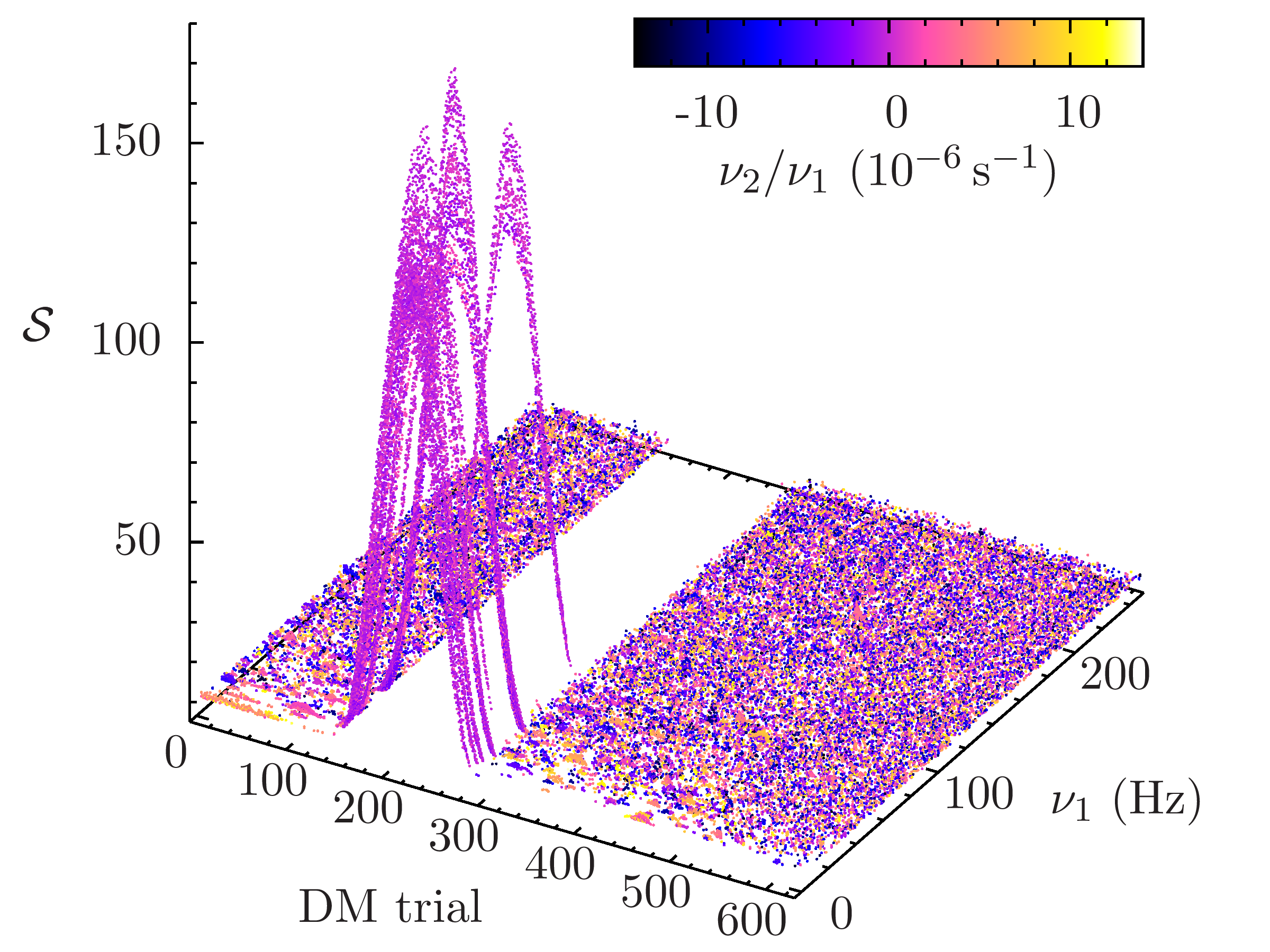
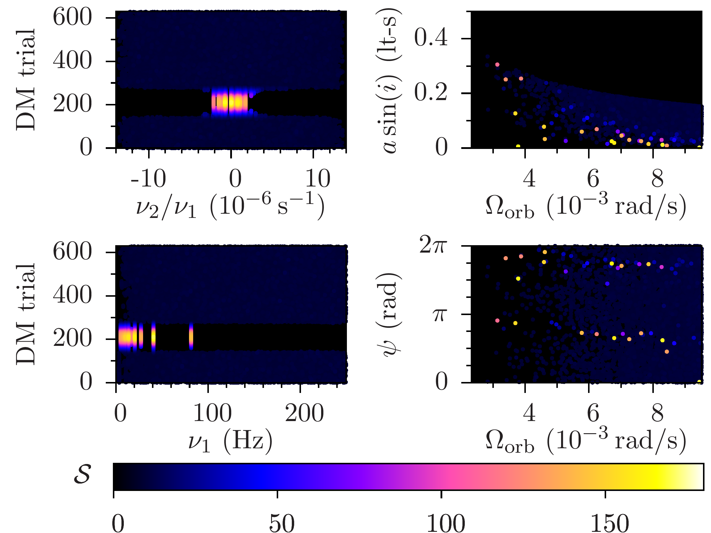
Figure 9.— Example post-processing overview plots, showing the highly-significant detection of PSR J2007$+$2722. Left: this plot shows the significance $\mathcal{S}$ as a function of the DM trial number and the fiducial spin frequency $\nu_{1}$ (see Section 4.16) of each candidate. The color-code displays the relative change in fiducial spin frequency $\nu_{2}/\nu_{1}$ from orbital motion. Since the top 100 candidates are reported for each DM trial and the pulsar is detected with very high significance, there are no detections of the noise floor in a DM range around the pulsar. Right: the four sub-panels show the significance $\mathcal{S}$ as a function of different combinations of spin frequency and the orbital parameters.

These plots use coordinates defined in the Appendix of Knispel et al. (2013). They are obtained from writing the phase model (1) as a power Taylor series in $t$. Then, the coefficient of the linear term $\nu_{1}=f\left(1+a\sin(i)\Omega_{\text{orb}}\cos\left(\psi\right)/c\right)$ identifies a spin frequency. The coefficient of the quadratic term $\nu_{2}=-a\sin(i)\Omega_{\text{orb}}^{2}f\sin\left(\psi\right)/(2c)$ is proportional to the Doppler spin-down or spin-up.

Promising candidates are identified from the visual inspection of these plots. The number of promising candidates is relatively small. The majority of PALFA beams have none; the most promising beams have at most a handful.

In the next step, PRESTO software tools are used to fold the full-resolution filterbank data for all candidates, starting with the spin-period and DM values identified from the Einstein@Home results. The prepfold plots are inspected by eye and used to judge the broadband nature and temporal continuity of the signal.

We also developed an automated routine which filters through the list of all candidates for a given beam and returns the most promising candidates. These candidates are then followed up automatically with different software tools described in detail in Knispel et al. (2013). The automated routine consolidates candidates at harmonically related frequencies, neighboring DMs, and similar orbital parameters. The remaining candidates are folded with prepfold to produce folded pulse profile and other diagnostic plots, as well as associated ASCII files. These are then filtered by a second piece of software, which uses these plots and ASCII files to select the most “pulsar-like” candidates (Knispel et al., 2013).

Using these two post-processing methods, the Einstein@Home search of the PALFA WAPP data made 322 detections of 158 unique radio pulsars. Of these pulsars, 156 were already known; they were listed in the ATNF catalog (Manchester et al., 2005), or on Web sites maintained by different ongoing pulsar surveys. Two of the pulsars, PSR J2007$+$2722 and PSR J1952$+$2630, were new; they appeared during the non-automated (visual inspection of the overview plots) post-processing.

5. Discovery of PSR J2007+2722

PSR J2007+2722 was found by project scientists on 2010 July 11 as part of the routine post-processing described in the previous section; the corresponding data had been acquired at Arecibo on 2007 February 11. In the post-processing plots (Figure 9) the pulsar appeared with maximum significance $\mathcal{S}=169.7$ at a dispersion measure DM=$127\,\text{pc\ cm}^{-3}$ and spin frequency of 40.821 Hz. The orbital parameters at highest significance were consistent with no orbital modulation, or with an orbital period longer than the longest orbital period in the template bank. In other words, it appeared that the pulsar was either isolated, or was in a long-period binary system. Further PRESTO-based analysis refined these values and supported the isolated or long-period interpretation.

The discovery was confirmed with a short Green Bank Telescope (GBT) observation soon thereafter, following which the pulsar was (re)observed at Arecibo, Jodrell Bank and Effelsberg. Details of later GBT studies are given in Section 6.2.2. A full timing analysis based on dozens of additional observations extending to late-2012 is given in Section 6.3.

Because the project database, and the result files themselves, contain information about the computers that carry out analysis, it is straightforward to identify the volunteers whose computers provide any particular result. As described in the Section 4.15 on validation, all Einstein@Home work is sent to computers owned by at least two different volunteers. In this case, the valid result files containing the statistics of highest significance for PSR J2007+2722 were returned by computers owned by volunteers from Ames, IA, USA and from Mainz, Germany.

The U.S. volunteers were Chris and Helen Colvin. For security reasons, the Colvins are not allowed to use their “work” computers for personal email and Web browsing, so they maintain a small mail and Web server at home. Since 2006, this home computer has been running Einstein@Home as a background job. The machine was equipped with an NVIDIA graphics card, whose GPU did the “discovery” processing.

The German volunteer was Daniel Gebhardt, who is the system administrator for a Musikinformatik group at Universität Mainz. Gebhardt runs a mail server for the group, which is continuously powered up, and runs Einstein@Home as a background task.

It is notable that the first discovery from the Einstein@Home pipeline, which was designed to find pulsars in binary systems, was an isolated pulsar, which was not found in either of the other PALFA processing pipelines. This is not unexpected: as described previously, the Einstein@Home search pipeline contains long-orbital period templates and one template with infinite period, so it can detect isolated systems. But why was it not found by the other pipelines?

In fact this is not surprising: the three pipelines in question (Einstein@Home, PRESTO and Cornell) produce statistical outlier candidate signals that are different owing to re-sampling differences, to differences in the way orbital motion is treated, and to the way signals that exceed statistical thresholds are reported. In total, each of these pipelines has involved about $10^{15}$ statistical tests so far, and the initial reduced set of candidate signals is in the millions. The three pipelines have different procedures and criteria for further winnowing these candidate signals into much shorter lists of viable pulsar candidates worthy of detailed visual inspection and follow-up observations at the telescope. The three pipelines also process the data in different order, and at the time of the PSR J2007+2722 discovery, all three had data backlogs: the fact of the matter is that the E@H pipeline found PSR J2007+27 first. Retrospectively, the pulsar could be seen in the output of one other pipeline (i.e. when we knew what to look for), while the other pipeline had not yet processed the relevant beam. In just the same way, the other pipelines have also found new pulsars that the E@H pipeline subsequently also detected.

5.1. Distance to PSR J2007+2722

Based on the NE2001 model (Cordes & Lazio, 2002) for the Galactic distribution of free electrons, the DM=$127\pm 0.4$ value implies a distance of 5.4 kpc. The uncertainty in distance arising from the 0.4 pc cm^-3 error in DM is negligible in comparison with the NE2001 model uncertainty. We know of two ways to bound this model uncertainty.

A direct measurement of errors in the NE2001 model can be obtained from comparisons of NE2001 distance estimates to actual parallax-based distance measurements (see Chatterjee et al. (2009, and references therein)). While direct comparisons are only possible for objects significantly closer than J2007+2722, for objects within 10^∘ of the pulsar, the parallax and DM distances agree to within 20%. Thus this direct measurement would suggests errors of less than 20% in the 5.4 kpc distance estimate.

To indirectly estimate the NE2001 model uncertainty, we first need to identify if an H II region or void perturbs the electron density along the line of sight, which would increase this uncertainty. In the case of PSR J2007+2722, we could not identify any specific H II region or source of radio recombination along the line of sight. The closest young star cluster on the sky is IRAS 20050+2720, about $20^{\prime}$ away from the line of sight and $\sim 0.7$ kpc distant from Earth. IRAS 20050+2720 has no massive stars that could produce a detectable H II region (Günther et al., 2012). IRAS and 5-GHz Very Large Array (VLA) images also do not show any extended emission near the line of sight. Thus, we estimate the NE2001 model uncertainties following the approach given in Section 4.2 and Figure 12 of Cordes & Lazio (2002). We assume that the DM is perturbed by subtle departures from the model at the level of $\Delta{\rm DM}=10$ and 20 pc cm^-3. These alter the inferred distance by $\pm 0.3$ and 0.6 kpc, respectively, corresponding to $\sim 6$% and 11% errors, or a maximum total error of 17%.

Choosing the worst case, we conservatively estimate the distance error to be less than 20%, and conclude that the distance of PSR J2007+2722 is $5.4\pm 1.1$ kpc.

6. Followup Observations and Characterization of PSR J2007+2722

6.1. Accurate Determination of the Sky Position

6.1.1 Gridding Observations with the Arecibo Telescope

The initial discovery of PSR J2007+2722 determined the sky position within about $2^{\prime}$: the Arecibo beam radius at 1.4 GHz. In normal circumstances, one determines pulsar positions more precisely using timing measurements over a period of a year or longer. Carefully fitting pulse arrival times to a timing model makes it possible to determine the sky position with an angular error $\delta\gamma\sim\epsilon P/D=3\times 10^{-8}$ radians, where $\epsilon\approx 10^{-2}$ is the typical time-of-arrival (TOA) error, measured as a fraction of the rotation phase, $P=1/f=25$ ms is the pulsar period, and $D\approx 10^{3}$ s is the light travel time across the diameter of the Earth’s orbit. This corresponds to a position error $\delta\gamma\sim 6$ milliarcsec; a timing-model position determination to such accuracy can be found in Section 6.3

However, the discovery of PSR J2007+2722 was an important milestone for Volunteer Distributed Computing, and waiting a year to precisely determine the sky position using timing was not an option. Nevertheless, we were able to narrow down the sky position using a combination of methods, in order to search for associated X-ray or gamma-ray sources and to set a limit on the magnitude of the spin-down $\dot{P}$. (If the TOA measurements cover much less than one year, then uncertainties/errors in sky position are degenerate with uncertainties/errors in $\dot{P}$.)

The first step in determining the sky position of PSR J2007+2722 more precisely was with a set of “gridding” measurements using the Arecibo telescope on 2010 July 19. The observations were done in S-band using the Mock spectrometers to construct five 172 MHz bands (center frequencies 2136, 2308, 2687, 2859, and 3013 MHz) with 1024 channels per band and a $65.5\leavevmode\nobreak\ \mu$s sampling time. A filter at the upper end of the S-band receiver bandwidth (band-passes at 2040-2400MHz and 2600-3100MHz) was used to minimize RFI and reduce the half-power beam width to $2^{\prime}$.

Decl. $\backslash$ R.A.	$20^{h}07^{m}18^{s}$	$20^{h}07^{m}14^{s}$	$20^{h}07^{m}10^{s}$
$27^{\circ}25^{\prime}26^{\prime\prime}$
$27^{\circ}24^{\prime}26^{\prime\prime}$	2.9	15.6	22.5
$27^{\circ}23^{\prime}26^{\prime\prime}$	19.8	97.9

Table 4 Arecibo gridding measurements used to refine the sky position of PSR J2007+2722. The pulsar was visible in five of the nine pointings; the table entries show the ratio of the folded profile peak to the rms noise floor.

The results of these first gridding measurements are shown in Table 4. A square grid of nine pointings was used, with the center at R.A. $20^{h}07^{m}14^{s}$ decl. $27^{\circ}24^{\prime}26^{\prime\prime}$, and the adjacent pointings offset by about $\pm 1^{\prime}$ ($\pm 4^{s}$ in RA and $\pm 1^{\prime}$ in decl.); the half-power beam contours overlapped by about $7^{\prime\prime}$ in R.A. As shown in the table, the pulsar was detected in five of the nine pointings. A weighted average of the two pointings with the largest S/Ns gave a position estimate R.A. $20^{h}07^{m}12^{s}.7$, decl. $27^{\circ}23^{\prime}26^{\prime\prime}$. We were confident that the pulsar was inside a $1^{\prime}$ radius circle about this point. A weighted average of all five pointings gives a position estimate differing by about $25^{\prime\prime}$, but might be biased since there are no observations to the south of the brightest grid point.

6.1.2 Observations with Westerbork Synthesis Radio Telescope

To further refine the sky position, observations were made with Westerbork Synthesis Radio Telescope (WSRT, Netherlands) at central frequency 1380 MHz with a 160 MHz bandwidth. WSRT is a linear array of 14 circular radio antennas, each 25m in diameter, arranged on a 2.7 km east-west line. Aperture synthesis creates a fan-beam approximately $12^{\prime\prime}\times 30^{\prime}$ in size, with the long axes along the north-south direction at transit. On the evening of 2010 July 19, ten 1180 s observations were made, with the center of each observation displaced by $12^{\prime\prime}$, as schematically shown in Figure 10. These covered the uncertainty region obtained from the Arecibo gridding observations. For each WSRT observation, the data were de-dispersed and folded with the PSR J2007+2722 period and DM using PuMa-II (Karuppusamy et al., 2008), a high time-resolution coherent de-dispersion pulsar-processing back-end. We believe this is the first time that WSRT has been used for pulsar position refinement in this way.

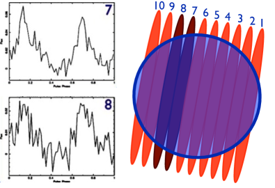
Figure 10.— Right: schematic illustration of 10 WSRT fan beams overlapped with the $1^{\prime}$-radius error circle obtained from gridding observations at the Arecibo observatory. The fan beam ellipses are not to scale: the minor axis is correct but the major axis is much longer than shown here. Left: folded pulse-profiles for fan beams 7 and 8 (horizontal axis is pulse phase, vertical axes is normalized flux). PSR J2007+2722 was not detected in any other fan beam.

The pulse profile was only convincingly detected in contiguous beams 7 and 8, with respective S/Ns 25 and 20, as shown in Figure 10. Weighted overlapping of fan beams 7 and 8 yields a position-constraint ellipse centered at R.A. $20^{h}07^{m}14^{s}.5$, decl. $27^{\circ}23^{\prime}36^{\prime\prime}$ as shown in Figure 11. The major and minor radii are $51^{\prime\prime}$ and $7^{\prime\prime}$; the major axis is rotated $20^{\circ}$ clockwise from North.

6.1.3 Westerbork Imaging and NVSS Catalog Sources

Simultaneously with pulsar data, WSRT imaging data were also acquired. Shown in Figure 11 is the radio image, along with the error ellipse just described. A single radio source is visible on the southern side of the error ellipse, just within the position circle obtained from the Arecibo gridding. This source is also listed in the 1.4-GHz National Radio Astronomical Observatory (NRAO) VLA Sky Survey (NVSS) catalog (Condon et al., 1998). The cataloged source NVSS 200715+272243 has coordinates R.A. $20^{h}07^{m}15^{s}.86$, decl. $27^{\circ}22^{\prime}43^{\prime\prime}.5$, a cataloged flux density of 2.3mJy at 1400 MHz, and an estimated size less than $3.3^{\prime\prime}$, consistent with the WSRT image.

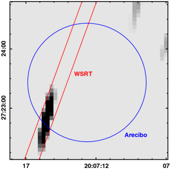
Figure 11.— An image of the WSRT data, along with the error circle obtained from Arecibo gridding, and the WSRT error region obtained by overlapping fan beams 7 and 8 as described in the text. The imaged source corresponds to a cataloged NVSS source and is PSR J2007+2722.

6.1.4 VLA Data Archive

It was possible to determine the position even more precisely from archival data. This part of the sky contains the young star cluster IRAS 20050+2720 (Günther et al., 2011). The VLA data archive contains a 1610 s on-source observation of IRAS2005 taken on 1997-08-14 (VLA project code AE0112A, data-set VLA_XH97065_file6.dat); the field of view (FOV) is approximately $16^{\prime}\times 16^{\prime}$. The data were acquired with the VLA C array operating in a 50 MHz bandwidth centered at 4.8601 GHz, in full Stokes mode, with a central beam position R.A. $20^{h}07^{m}05^{s}.859$, decl. $27^{\circ}28^{\prime}59^{\prime\prime}.77$.

We analyzed the full FOV using MAXFIT to characterize the eight point sources and one extended source which are visible above the background noise. Shown in Figure 12 is the part of this data (about $10^{\prime}\times 14^{\prime}$) containing the sources, which are circled.

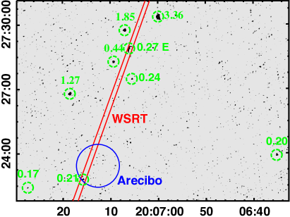
Figure 12.— An image of (a part of the) archival VLA data at 4.8 GHz. To compensate for the drop-off in sensitivity near the edge of the primary beam, the intensity has been divided by a model for primary beam response. The intensity has an rms of 42 $\mu$Jy; there are nine sources brighter than 170 $\mu$Jy, which are shown in the dashed circles. The source fluxes determined by MAXFIT are given in mJy, before dividing by the beam response; the extended source is indicated by “E”. The larger circle is the $1^{\prime}$-radius source uncertainty region found by the Arecibo gridding and the region between the two “parallel lines” is the relevant portion of the uncertainty ellipse found by the WSRT gridding. There is only one source (PSR J2007+2722) lying in both uncertainty regions; it has a unnormalized flux of $210\,\mu$Jy and a normalized flux of $1.2$ mJy.

As can be clearly seen in Figure 12, only one of these (point) sources lies inside the uncertainty regions obtained from the WSRT and Arecibo observations. This is shown in more detail in Figure 13. The point source has coordinates R.A. $20^{h}07^{m}15^{s}.77$, decl. $27^{\circ}22^{\prime}47^{\prime\prime}.68$ and an uncorrected flux density of $0.21$ mJy; the primary beam-corrected flux density is 1.2 mJy ($\pm 10$%) at 4.86 GHz. (The absolute flux density measurement is referred to 3C48; the errors arise primarily from uncertainties in the primary beam model, because the source is close to the edge of the beam.) The flux density is consistent with the normal spectral behavior of similar radio pulsars; we conclude that this is the correct location of PSR J2007+2722.

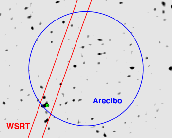
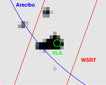
Figure 13.— Archival VLA data at 4.8 GHz. Top: a $180\times 144^{\prime\prime}$ region with the 1’-radius uncertainty region from Arecibo gridding and the 13”-wide uncertainty region from WSRT gridding; the overlap contains a single VLA source (small circle). Middle: a $30\times 24^{\prime\prime}$ zoom showing the 1.2 mJy VLA source near the south side of the previous region. The 1”-radius circle shows the uncertainty region obtained by fitting a Gaussian to the VLA intensity; the discovery publication used this as the PSR J2007+2722 position. Bottom: a $5\times 4^{\prime\prime}$ zoom; the cross indicates the location of PSR J2007+2722 obtained in this paper by timing analysis. It lies inside the 1”-radius VLA uncertainty region. The intensity scale has been changed in the bottom plot to show the brightest VLA pixels.

6.2. Multi-frequency Observations and Emission Geometry

6.2.1 Arecibo Observations at 327 and 430 MHz

Early observations of PSR J2007+2722 at 327 and 430 MHz did not see convincing evidence of pulsations. It turned out that the issue was instrumental: more extended observations at Arecibo Observatory in Spring 2013 did succeed.

On 2013 April 16, the pulsar was observed for 960 s from 420-447 MHz, using the Mock spectrometer in search mode with 1024 channels covering 34 MHz bandwidth, and a 119 $\mu$s sample time. The data were rescaled and converted from 16-bit PSRFITS to 4-bit PSRFITS, then folded using presto with the ephemeris of Section 6.3. Channels falling outside the 27 MHz receiver bandwidth were discarded. After folding, the profile was calibrated with respect to the measured system gain (11 K/Jy) and noise equivalent temperature of 115K. Pulsations were observed with a false alarm probability corresponding to $4.0\,\sigma$.

The noise equivalent temperature was determined from measurements on April 17, using a diode noise source calibrated against hot- and cold-loads of known temperature. These yielded 75K at high Galactic latitudes and 115K close to the Galactic plane. The 40K difference is consistent with the 408 MHz measurements and models of Haslam et al. (1982): extrapolation to 430 MHz using spectral slope $T_{\rm sky}\propto f^{-2.3}$ predicts a 44K Galactic contribution.

On April 30 the pulsar was observed for 1761 s from 290-359 MHz. We used the Puertorican Ultimate Pulsar Processing Instrument (PUPPI) backend operating in search mode with a 81.92 $\mu$s sample time. This PUPPI mode nominally covers 100 MHz of bandwidth in 4096 channels, but only 2816 channels covering the 69 MHz receiver bandwidth were recorded. The data were folded and calibrated as above, using a measured equivalent noise temperature of 186 K and gain of 11 K/Jy. Pulsations were observed with a false alarm probability corresponding to $5.5\,\sigma$.

The equivalent noise temperature was determined using calibrated measurements away from the Galactic plane (which yielded 100-105K, and adding the estimated Galactic background contribution of 83K, obtained as above from Haslam et al. (1982).

Pulse profiles from these observations are shown in the bottom two plots of Figure 14; rotation-averaged pulsed fluxes derived from these are given in Table 5.

6.2.2 Green Bank Telescope Observations

The GBT carried out follow-up observations on 2010 July 21, in bands centered at 820, 1500, 2000, and 8900 MHz. Full Stokes data were obtained for the observations at 1500, 2000, and 8900 MHz, but the 8900 MHz data was too noisy to be useful for polarimetry.

All GBT observations of PSR J2007$+$2722 were carried out using the Green Bank Ultimate Pulsar Processing Instrument (GUPPI) in incoherent de-dispersion mode. The observations at 820 MHz used 200 MHz total bandwidth, 2048 spectral channels and 40.96 $\mu$s time resolution. For the 1500 MHz and 2000 MHz observations, 800 MHz total bandwidth, 2048 channels and 25.6 $\mu$s time resolution were used. At 8900 MHz, the parameters were 512 channels, 800 MHz bandwidth and 6.4 $\mu$s time resolution.

The total observation time at each frequency was approximately 30 minutes. Along with each pulsar observation, a short amount of data were recorded with the local calibration-noise source pulsed at 25 Hz. The equivalent noise source flux in each polarization channel was determined by observing standard astronomical flux calibration sources (3C190 was used at 820, 1500, and 2000 MHz; 3C48 at 8900 MHz). The noise source measurements were then used for polarimetric calibration (differential gain and phase) and absolute flux calibration of the pulsar data. All data processing described in this section was performed using the PSRCHIVE software package (Hotan et al., 2004).

The pulse profile of PSR J2007+2722 is unusually broad: at 1500 MHz the full pulse width between the outer half-maxima is $\approx 224^{\circ}$. The folded pulse profiles at the four GBT observed frequencies are shown in the top four plots of Figure 14. All observations exhibit a double-peaked pulse profile with an emission bridge between and connecting the two peaks. The emission bridge flattens with increasing observation frequency and shifts location from between the peaks at lower frequency to outside the peaks at 8900 MHz. This indicates that some radio emission is present at all rotational phases in addition to the pulsed emission.

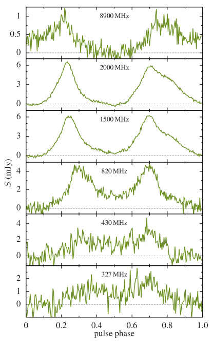
Figure 14.— The pulse profile in mJy at 327, 430, 820, 1500, 2000, and 8900 MHz. The rotation-averaged pulsed flux is given in Table 5. All the plots show an emission “bridge” between the two pulses, which shifts to outside the peaks at the highest frequency. This is evidence that the pulsar is “always on”, suggesting that the pulsed flux shown in Table 5 is only a fraction of the total flux.

For all frequencies at which the pulsar was detected, pulse-averaged flux densities were obtained. In combination with the flux density from the NVSS catalog and the VLA archival data, the pulsar’s flux density has been measured at eight different frequencies. Table 5 summarizes these measurements.

Frequency (MHz)	Flux Density (mJy)	Pulsed/Total?	Instrument
327	0.6	P	Arecibo
430	1.0	P	Arecibo
820	1.6	P	GBT
1400	2.3	T	NVSS Catalog
1500	2.1	P	GBT
2000	1.7	P	GBT
4860	1.2	T	VLA Archive
8900	0.3	P	GBT

Table 5 Flux density of PSR J2007+2722 at different frequencies. The pulsed measurements (P) only show the (rotation-averaged) component of the flux density that varies with pulse phase, referred to the dashed baseline in Figure 14. The total measurements (T) also include the phase-independent part. The VLA/NVSS flux measurements are described in Section 6.1.3, and the GBT and Arecibo measurements in Section 6.2.2.

The flux density measurements from the Arecibo Telescope and GBT observations are only sensitive to the pulsed emission. Fitting a single-component power law

$$S\left(\nu\right)=S_{1400}\left(\frac{\nu}{1400\,\textrm{MHz}}\right)^{\xi}$$ (18)

to measurements of the pulsed flux density $S$ at frequencies $\nu>$1 GHz, we obtain a spectral index $\xi=-1.12(6)$, i.e. a relatively flat spectrum (Lorimer & Kramer, 2004).

The low pulsed-flux density below 1400 MHz is unusual, as pulsar spectra generally turn over at frequencies around $\sim$100 MHz. Unless the non-pulsed flux dominates the pulsed flux, PSR J2007+2722 belongs to the small subset of pulsars with GHz-peaked spectra. Kijak et al. (2011) suggest that this behavior could be due to unusual environments, since PSR B1259-63 exhibits such a spectrum at periastron. While only 5 such sources have been reported thus far, Bates et al. (2013) estimate that they may comprise up to 10% of the pulsar population. However, more such objects are necessary to draw any reliable conclusions.

6.2.3 Polarimetry

The GBT observations also provided full Stokes polarization parameters $I$, $Q$, $U$, and $V$ at 1500 and 2000 MHz, from which the polarization angle

$$\psi=\frac{1}{2}\arctan\left(\frac{U}{Q}\right)$$ (19)

can be computed as a function of the pulsar rotation phase. These polarization-angle profiles are shown in Figure 15 as a function of pulsar rotation phase, along with estimated measurement uncertainties $\Delta\psi$. We use PSR/IEEE sign conventions for $\psi$ and $V$, as defined by van Straten et al. (2010) and employed by PSRCHIVE.

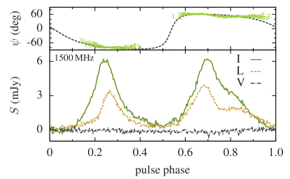
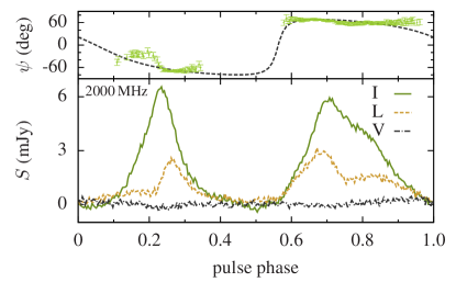
Figure 15.— Full Stokes polarization-angle profiles at 1500 MHz (top) and 2000 MHz (bottom) taken at GBT. The horizontal axis is rotation phase of the pulsar. The bottom half of each plot shows the radio flux-density $S$ in intensity $I$ (solid), linearly polarized component $L=\sqrt{U^{2}+Q^{2}}$ (dashed) and circularly polarized component $V$ (dash-dotted). The top half of each plot also shows the derived polarization angle $\psi$ from Equation (19), corrected with rotation measure RM$=-230$ for Faraday rotation arising from the Galactic magnetic field . The dashed lines show $\psi_{\textrm{RVM}}$ for the best-fit rotating vector models given by Equation (6.2.4) and Table 6.

6.2.4 Emission/Beam Geometry

The polarization-angle profiles can be used to infer the beam geometry from the Rotating Vector Model (RVM; Radhakrishnan & Cooke, 1969). In the RVM, the beam geometry is defined by four free parameters: $\alpha$, $\zeta\equiv\alpha+\beta$ , $\psi_{0}$ and $\phi_{0}$. Here, $\alpha$ is the angle from the spin vector to the “visible” magnetic axis, and $\zeta$ is the minimum angle from the spin vector to the pulsar-observer line of sight. These angles are described and illustrated in Figure 1 of Everett & Weisberg (2001), whose conventions we adopt. The polarization angle at pulsar rotation phase $\phi_{0}$ is denoted $\psi_{0}$.

The polarization angle $\psi_{\textrm{RVM}}$ as a function of the pulsar’s rotation phase $\phi$ is

$$\tan\left(\psi_{\textrm{RVM}}-\psi_{0}\right) =$$

$$-\,\frac{\sin\left(\phi-\phi_{0}\right)\sin\left(\alpha\right)}{\sin\left(\zeta\right)\cos\left(\alpha\right)-\cos\left(\zeta\right)\sin\left(\alpha\right)\cos\left(\phi-\phi_{0}\right)}.$$

The sign on the rhs occurs because we follow the “observer’s” or “IAU/IEEE” convention for which the polarization angle $\psi$ increases in the counter-clockwise direction on the sky, as detailed in Everett & Weisberg (2001). This polarization angle convention is the same as PSR/IEEE (van Straten et al., 2010).

The values of the four RVM parameters were determined by a least-squares fit. We began with the measurements of the polarization angle $\psi$ for $N_{1500}=158$ different values of the rotation phase at 1500 MHz, and for $N_{2000}=143$ different values of the rotation phase at 2 GHz, as shown in the upper parts of Figure 15. At each point of a 4-dimensional cubical grid (spacing $0^{\circ}.5$) in $\left(\alpha,\zeta,\psi_{0},\phi_{0}\right)$-space, we calculated the normalized sum of the squared-residuals,

$$\chi^{2}=\frac{1}{N-4}\sum_{i=1}^{N}\frac{\left(\psi(\phi_{i})-\psi_{\textrm{RVM}}(\phi_{i})\right)^{2}}{(\Delta\psi_{i})^{2}},$$

between the RVM-predicted and measured polarization angles. Here $i$ labels the $N=N_{1500}$ or $N=N_{2000}$ distinct pulsar rotation phases $\phi_{i}$ for which $\psi_{i}=\psi(\phi_{i})$ was measured, and $\Delta\psi_{i}$ is the experimental measurement uncertainty in $\psi_{i}$.

Because the number of degrees of freedom is $N-4$, $\chi^{2}$ is a conventionally-normalized reduced-chi-squared statistic. Values of $\chi^{2}$ near unity indicate that RVM fits the data well (consistent with Gaussian-distributed errors of standard deviation $\Delta\psi$ in the values of $\psi$). Large values of $\chi^{2}$ indicate a poor fit. Figure 16 shows the minimum value of $\chi^{2}$ as a function of $\left(\alpha,\zeta\right)$; note that the color code has a logarithmic scale. The minimum $\chi^{2}$ values obtained over all four parameters, and the corresponding best-fit parameter values, are shown in Table 6. These best-fit values are shown by black crosses in Figure 16.

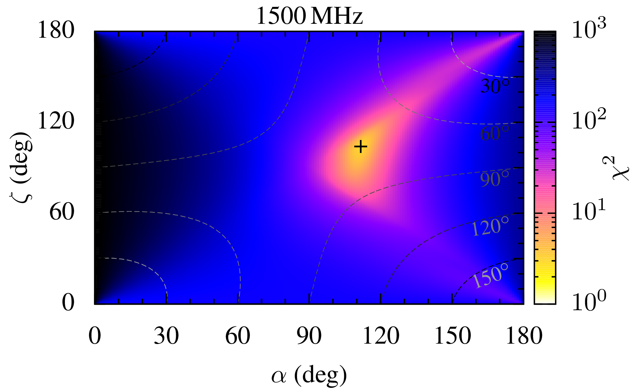
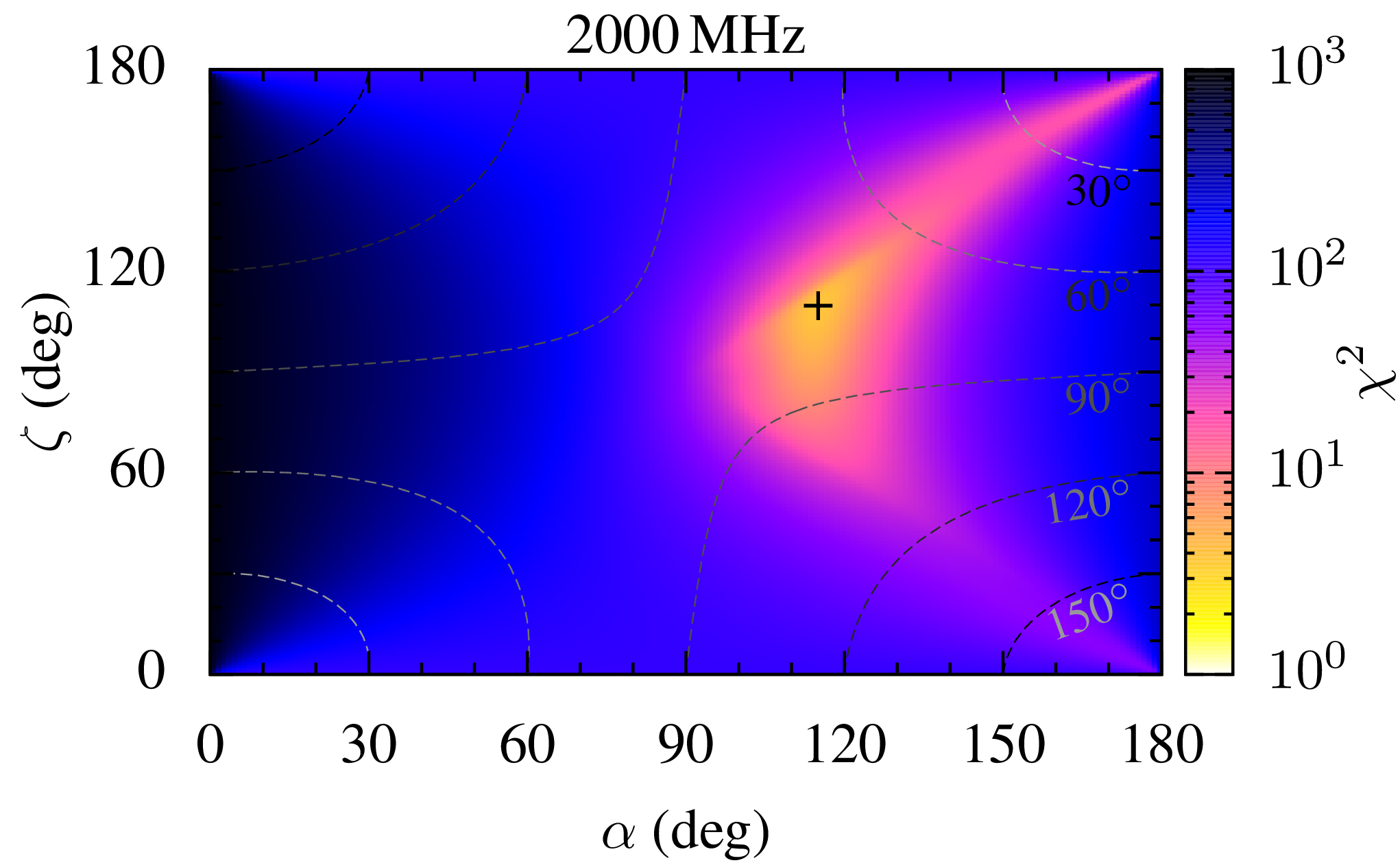
Figure 16.— The reduced chi-squared values $\chi^{2}$ as a function of ($\alpha$, $\zeta$), obtained by fitting the measured polarization angle to the RVM model Equation (6.2.4) as described in the text. At each point the $\chi^{2}$ was minimized over $\phi_{0}$ and $\psi_{0}$. The dashed lines are the contours of constant emission-cone half-opening-angle as defined by Equation (21).

Frequency	$\alpha$	$\beta$	$\phi_{0}$	$\psi_{0}$	$\chi^{2}$
1500 MHz	$111.7(5)^{\circ}$	$-7(1)^{\circ}$	$192(2)^{\circ}$	$12.7(8)^{\circ}$	3.13
2000 MHz	$115.1(8)^{\circ}$	$-5(1)^{\circ}$	$202(3)^{\circ}$	$5(2)^{\circ}$	3.74

Table 6The best-fit RVM parameters for PSR J2007+2722 obtained from fitting the model in Equation (6.2.4) to the measured polarization angle as a function of pulsar rotation phase. $\chi^{2}$ is the minimum reduced-chi-squared value, and the numbers in parentheses are the estimated 1 $\sigma$ errors.

The corresponding best-fit polarization-angle profiles are displayed by dashed lines in the top panels of Figure 15. The fit is acceptable in the sense that it is not untypical when compared with other radio pulsars. Overall, the RVM reproduces the form of the observed profile, especially at 1500 MHz, but leaves unmodeled structure below pulse phase 0.2 and above pulse phase 0.9. The largest deviations are at 2000 MHz below phase 0.25. Nevertheless it is encouraging that the independent fits at 1500 and 2000 MHz lead to very similar beam geometry parameters, and surprisingly tight bounds on their values, as shown in Table 6.

However the fit can not be characterized as good; the deviations between data and model that are visible in Figure 15 give rise to reduced-chi-squared $\chi^{2}$ values that have very low statistical likelihood of being explained by the polarization-angle measurement errors. The failure to fit the RVM very well may arise because the pulsar does not ever “shut off” but is emitting over its entire rotation. This can affect the polarimetry; in Figure 15 one can see regions where the intensity $L$ of the linearly-polarized component is greater than the total intensity $I$. This can not happen in nature; the inconsistency probably indicates that some aspect of the polarimetry measurement can not be trusted. It could well be an artifact of not being able to identify the uniform level of flux corresponding to zero pulsed emission. However the lack of a good fit is also consistent with the interpretation that PSR J2007+2722 is a DRP: many recycled pulsars are not well-fit by the basic RVM (Thorsett & Stinebring, 1990; Navarro et al., 1997; Xilouris et al., 1998; Stairs et al., 1999).

One can infer the opening-angle of the radio emission-cone from the RVM parameters together with the observed separation between the pulse peaks. The emission-cone half-opening-angle $\rho$ is related to the measured separation $W$ of the pulse peaks by

$$\cos\left(\rho\right)=\cos\left(\alpha\right)\cos\left(\zeta\right)+\sin\left(\alpha\right)\sin\left(\zeta\right)\cos\left(\frac{W}{2}\right).$$ (21)

At 1500 MHz we estimate a peak-to-peak width of the pulse profile $W_{1500}=163^{\circ}$; at 2000 MHz $W_{2000}=171^{\circ}$. For these values of $W$, the dashed lines in Figure 16 show contours of constant emission-cone half-opening-angle $\rho$ as a function of $\alpha$ and $\zeta$. Using the best-fit $\alpha,\zeta$ values from Table 6 we obtain radio-emission-cone half-opening-angles $\rho_{1500}=77^{\circ}$ and $\rho_{1500}=78^{\circ}$ at 1500ṀHz and 2000 MHz, respectively.

6.3. Timing Model

A timing model for PSR J2007+2722 has been found using two distinct data sets, obtained at the Arecibo Observatory and at Jodrell Bank. The Arecibo data were collected in two short (268 s) survey observations on 2007 February 11 and 16; the first of these provided the data used in the Einstein@Home discovery. The Jodrell data were collected in 75 targeted observations between 2010 July 15 and 2012 November 30, starting soon after the discovery.

The Arecibo data (described earlier) covering a 100 MHz bandwidth centered at 1452 MHz, were used to construct TOAs in four distinct 25 MHz frequency bands. A model pulse profile was used to obtain 22 distinct TOAs.

The Jodrell Bank observations used a dual-polarization cryogenic receiver on the 76-m Lovell telescope, having a system equivalent flux density of 25 Jy on cold sky. Observations typically lasted 20 or 30 minutes. Data were processed using a digital filterbank which covered a bandwidth of 350 MHz centered around 1525 MHz in channels of 0.5 MHz bandwidth. The data were folded at the nominal topocentric period of the pulsar for sub-integration times of 10 s. After inspection and removal of any RFI, the profiles were de-dispersed and summed over frequency and time to produce integrated profiles. For each observation, a single TOA as obtained by cross-correlation of the profile with a standard template using standard analysis tools from PSRCHIVE.

The 97 distinct TOAs were analyzed using the TEMPO2 software package (Hobbs et al., 2006; Edwards et al., 2006). In the fitting procedure to determine the pulsar parameters, a single adjustable offset time (TEMPO2 “jump”) was introduced between the two data sets. This is needed because different model pulse profiles were used to derive the Arecibo and Jodrell TOAs, and avoids the need for absolute time synchronization between the two observatories.

The parameters of PSR J2007+2722 obtained from this TEMPO2 analysis are shown in Table 7; the resulting fitting residuals are shown in Figure 17. The fit is remarkably good: the residuals have a weighted rms of 66 $\mu$s and the reduced $\chi^{2}=1.059$ is very close to unity. In pulsar astronomy it is standard practice to re-scale the uncertainties by the square-root of this value; we have done that here, but it only changes the estimated one-sigma errors by about 3%.

The pulsar parameters obtained by timing (sky position, frequency, and spindown) are reasonably consistent with the announcement paper (Knispel et al., 2010) published one month after the discovery. That paper gave the sky position (found as described in Section 6.1) as R.A. $\rm 20^{h}07^{m}15^{s}.77$, decl. $\rm 27^{o}22^{\prime}47^{\prime\prime}.7$ with errors less than order $1^{\prime\prime}$. The position found here is consistent with that. The discovery paper gave the frequency (at MJD 55399) as $f=\rm 40.820677620(6)\,$Hz. The frequency found here is about one standard deviation outside of that range; this may have been due to our lack of knowledge about the precise spin-down rate. Finally, the discovery paper only gave a bound on the spin-down rate, of $|\dot{f}|<3\times 10^{-14}/\rm s^{2}$. The spin-down found here is consistent with that: $\dot{f}=-1.6\times 10^{-15}/\rm s^{2}$. This corresponds to a characteristic age $-f/2\dot{f}=\rm 404\,$Myr, an inferred surface dipole magnetic field strength of $4.9\times 10^{9}\,$G, and a spin-down luminosity $\dot{E}=2.6\times 10^{33}$ erg/s (assuming the canonical moment-of-inertia $I=10^{45}\leavevmode\nobreak\ \text{g}\leavevmode\nobreak\ \text{cm}^{2}$).

Figure 17.— Timing residuals obtained by fitting a timing model to TOA data from Arecibo Observatory (taken in 2007 February) and TOA data from Jodrell Bank (taken between 2010 July and 2012 November). The horizontal axis is the date of the TOA observation, and the vertical axis is post-fit residuals in seconds.

Fit and data-set
Pulsar name	JJ2007+2722
MJD range	54142.7—56261.4
Number of TOAs	97
Rms timing residual ($\mu s$)	65.6
Weighted fit	Y
Reduced $\chi^{2}$ value	1.057
Measured quantities
Right ascension, $\alpha$	20:07:15.8288(4)
Declination, $\delta$	+27:22:47.914(6)
Pulse frequency, $\nu$ (s-1)	40.820677605083(15)
First derivative of pulse frequency, $\dot{\nu}$ (s-2)	$-$1.6015(4)$\times 10^{-15}$
Dispersion measure, $DM$ (cm-3pc)	127.0(4)
Set quantities
Epoch of frequency determination (MJD)	55399
Epoch of position determination (MJD)	55399
Epoch of dispersion measure determination (MJD)	55399
Derived quantities
$\log_{10}$(Characteristic age, yr)	8.61
$\log_{10}$(Surface magnetic field strength, G)	9.69
$\log_{10}$(Canonical spin-down luminosity, erg/s)	33.4

Table 7The parameters describing PSR J2007+2722 obtained by timing analysis of data spanning about six years using a DE405 solar-system ephemeris model. Figures in parentheses are the nominal 1$\sigma$ tempo2 uncertainties in the least-significant digits quoted. For easy comparison, the Epoch has been chosen to be the same as Knispel et al. (2010) rather than at the midpoint of the observational interval.

6.4. Multi-wavelength Electromagnetic Counterparts

With the final sky position given in Table 7, we searched for electromagnetic counterparts at different wavelengths. The pulsar is not in any known globular cluster or near a cataloged supernova remnant (Green, 2009). We then checked infrared, gamma-ray and X-ray catalogs for counterparts. Infrared: The nearest sources visible in infrared images (J, H, K-band) obtained from the Two Micron All Sky Survey (Skrutskie et al., 2006) are more than $13^{\prime\prime}$ distant from the pulsar position. Gamma-ray: No counterpart was found in the second Fermi LAT Point Source Catalog (Nolan et al., 2012). X-ray: There are three archival Chandra X-ray observations; from these, no X-ray counterpart could be identified. We then carried out more detailed followups starting from the raw gamma-ray and X-ray data as described below.

Since the launch of Fermi in 2008, the on-board LAT (Atwood et al., 2009) has observed pulsations from more than 120 pulsars, and new blind-search methods similar to those used in this paper are finding even more (Pletsch et al., 2012b, c, a). The LAT has also confirmed that many radio-detected, both normal and millisecond, pulsars are emitting rotation-phase-synchronous gamma-rays (Abdo et al., 2009; Ray et al., 2012). So, we here consider the possibility of PSR J2007+2722 also being a gamma-ray pulsar.

Unfortunately the characteristics of PSR J2007+2722 make it an unlikely source for gamma-ray emissions or pulsations, when comparing to the known gamma-ray pulsar population Abdo et al. (2013). Its spin-down power $\dot{E}=2.6\times 10^{33}$ erg/s is near the lower end of the known gamma-ray pulsar population, and at a distance of $d=5.4$ kpc, the spin-down flux density $\dot{E}/d^{2}$ is smaller than that of any known gamma-ray emitting pulsar by a factor of a few. In addition, PSR J2007+2722 is in a high-background region close to the Galactic plane. The Fermi-LAT Second Source Catalog (Nolan et al., 2012) does not contain any source positionally overlapping with the pulsar’s location.

Nevertheless, we searched the LAT data for gamma-ray pulsations synchronous with the radio-pulse rotation phase. We extracted the LAT photons within $2^{\circ}$ of PSR J2007+2722’s sky position from the start of data taking in 2008 August up to 2013 January. We folded them for different cuts on minimum energy (between 40 MeV and 0.8 GeV) and different angular cuts (between $0.5^{\circ}$ and $2^{\circ}$). There was no sign of a signal; the LAT does not detect gamma-ray pulsations from PSR J2007+2722. In principle, one could carry out a spectral analysis of the region and construct a source model for PSR J2007+2722 to assign probability weights to the LAT photons as in Pletsch et al. (2012b). However, given the extremely low pulsation significance of the unweighted fold, we concluded this was unlikely to make much of a difference.

6.5. X-ray Limits, and the Nature of PSR J2007+2722

Figure 18.— The population of known radio pulsars, plotted as a function of spin-period (horizontal axis) and rate of change of the spin-period with time (vertical axis). PSR J2007+2722 is at the intersection of the dotted lines: a region populated almost exclusively by old recycled pulsars in binary systems, indicated by circled points. In contrast to PSR J2007+2722, almost all isolated pulsars (uncircled points) are in the region populated by much younger non-recycled systems.

As shown in Figure 18, timing measurements of PSR J2007+2722 place it in a region of the ($P,\dot{P}$)-diagram normally occupied by old neutron stars in binary systems spun-up due to accretion torques (i.e. “recycled”). These pulsars naturally have shorter periods ($P\mathrel{\hbox{\hbox to0.0pt{\hbox{\lower 4.0pt\hbox{$\sim$}}\hss}\hbox{$<$}}}100$ ms) than the younger, isolated rotation-powered pulsars and are constrained to lie below the spin-up limit for recycled pulsars $P({\rm ms})=1.9(B/10^{9}\ {\rm G})^{6/7}$ (van den Heuvel, 1987), where the magnetic field restricts the minimal achievable rotation period.

Together with the lack of a stellar companion at any wavelength or unmodeled systematics in the timing residual to indicating otherwise, there is no evidence that PSR J2007+2722 is currently part of a binary system. Instead, its moderately short period suggests that it was partially recycled and is possibly a DRP. These isolated neutron stars are born in a binary system and become unbound by a second supernova event involving the companion; they are defined in Belczynski et al. (2010) as isolated radio pulsars in the Galactic disk with magnetic field strength $|B|<3\times 10^{10}$ G and spin-frequency $f<50$ Hz. Their evolutionary origin explains their location on the region of the ($P,\dot{P}$)-diagram which is populated by weak magnetic field pulsars, whose fields have decayed over $\sim 10^{8}$ yr. The work by Belczynski et al. (2010) describes the 12 DRPs known at the time of publication; one more (PSR J1821+0155) has subsequently been discovered (Rosen et al., 2013). PSR J2007+2722 would be the 14th and most rapidly spinning member of this class.

DRPs are an enigma: standard evolutionary models for binary systems cannot easily explain the observed ratio of isolated recycled pulsars relative to the number of DNS systems (Belczynski et al., 2010). The models predict about DNS system for every ten DRPs, but roughly equal numbers are observed. Furthermore, there is no independent evidence that all isolated pulsars overlapping the binary population are actually derived from binaries. Indeed, recent observations of manifestly young pulsars in supernova remnants reveal that neutron stars can be born with anomalously low surface dipole magnetic fields of order $B\sim 10^{10}$ G (see Gotthelf et al. 2013b for details). These so-called anti-magnetars occupy an overlapping region in the ($P,\dot{P}$)-diagram with the DRPs and therefore suggest that their descendants might be mis-identified as DRPs (Gotthelf et al., 2013a). If in fact PSR J2007+2722 is a young object instead of a $\sim 10^{8}$ yr-old DRP, neutron star cooling curves predict that thermal X-ray surface emission should be observable for up to 1 Myr (Page et al., 2009), long after its supernova remnant has dissipated. After this time, the internal temperature drops rapidly and thermal emission becomes negligible.

To investigate the possibility that PSR J2007+2722 might be a young, hot object, we examined fortuitous archival X-ray observations covering the location of the pulsar. A total of 95 ks of good Chandra/ACIS-I data are available as data sets ObsIDs 6438, 7254 and 8492, acquired on 2006 December 10, 2007 January 07 and 29, respectively (Günther et al., 2012). The expected location of the pulsar falls $6^{\prime}$ off-axis for each observation, where the point response function of the telescope is degraded to $5^{\prime\prime}$ ($99\%$ enclosed energy fraction). Within the nominal absolute astrometry error of $0\farcs 6$ radius no X-ray source is found that overlaps with the subarcsec pulsar coordinates presented herein. As shown in Figure 19, the closest source is $14\farcs 3$ away from PSR J2007+2722.

To attempt to place a lower limit on the age of PSR J2007+2722 we use the Chandra data to determine the minimum detectable flux expected from a cooling neutron star of radius $R=14$ km at the DM derived distance of 5.4 kpc. Following the method described in Gotthelf et al. (2013a), we compute an upper-limit on the number of expected counts for a non-detection at the $99.73\%$ confidence level ($3\sigma$). Based on the local background rate of $1.6\times 10^{-5}$ cps in the $r=5^{\prime\prime}$ aperture, we require 6.5 photons from the pulsar in the composite ACIS-I observation in the $0.3-2$ keV energy band at the off-axis pulsar location. We convolve an absorbed blackbody spectrum with the telescope response function generated for these observations and integrate over the energy band to compute the detected number of counts as a function of temperature. The blackbody normalization is fixed to the ratio of the neutron star radius to its distance and the column density is set to $N_{\rm H}\approx 4\times 10^{21}$ cm^-2, estimated from the DM and by assuming a rule-of-thumb $N_{e}/N_{\rm H}\sim 0.1$. This procedure yields a temperature of $k{\rm T}\approx 69$ eV and bolometric luminosity of $L({\rm bol})\approx 6\times 10^{32}$ erg s^-1 implying a lower limit on the neutron star cooling age $\mathrel{\hbox{\hbox to0.0pt{\hbox{\lower 4.0pt\hbox{$\sim$}}\hss}\hbox{$>$}}}1-5\times 10^{5}$ yr, depending upon the range of cooling-curve models (Page et al., 2009). This luminosity is less than 10% of what would be expected for a typical young neutron star.

The uncertainty in this upper limit on luminosity is difficult to estimate. The contribution from the unknown column density depends on the uncertainty in the Galactic electron density distribution, estimated as 20% in Cordes & Lazio (2002). A recent calibration of the ratio $N_{e}/N_{\rm H}$ shows over an order-of-magnitude scatter in this relationship (He et al., 2013). If $N_{\rm H}$ varied by an order-of-magnitude away from our assumed value, then the lower limits on the age could be as small as $10^{4}$ yr. Moreover, the effects of any uncertainty on $N_{\rm H}$ are amplified because the derived temperature falls at the edge of the ACIS-I response function where the detector sensitivity falls off rapidly.

It appears unlikely that PSR J2007+2722 is a young pulsar, but current data cannot prove that it was formed through recycling in a binary system versus being simply an isolated pulsar born with a low magnetic field. For a typical rotation-powered pulsar emitting non-thermal X-rays with power-law spectrum of photon index $\Gamma=1.5$, the $2-10$ keV luminosity upper limit for PSR J2007+2722 is $2.2\times 10^{31}$ erg s^-1. However, based on its spin-down energy of $\dot{E}=2.58\times 10^{33}$ erg s^-1, the predicted X-ray luminosity in this band is only $L_{\rm x}=2.7\times 10^{29}$ erg s^-1 (Possenti et al., 2002). So no definite constraint is possible.

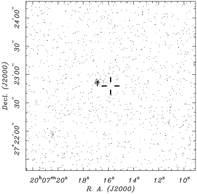
Figure 19.— Chandra ACIS X-ray image ($0.3-2$ keV) of the field containing PSR J2007+2722, whose location is marked by the cross. The field-of-view is $3^{\prime}\times 3^{\prime}$. The nearest resolved point source is $14\farcs 3$ away.

7. Discussion and Conclusions

We have presented a detailed description and full timing model for PSR J2007+2722, the first Einstein@Home radio pulsar discovery. Evidence from polarization studies, lack of associated remnants, and its location on the $(P,\dot{P})$ diagram, support the hypothesis that it is a DRP, about 0.4 Gyr old. However there remains the possibility that it is a much younger object born with a low magnetic field. In this case it is probably at least 100 kyr old.

PSR J2007+2722 has other unusual properties. Its (pulsed) radio spectrum peaks at higher (GHz) frequencies than most pulsars, and has a relatively flat spectral index above 1 GHz. The pulse profile is remarkably wide with emission over almost the entire spin period, and the beam geometry is well constrained by the RVM. The beam geometry is also atypical: the pulsar is almost an orthogonal rotator, the magnetic field axis passes quite close to the line-of-sight and the beam opening angle is unusually broad.

We have also given a detailed description of the Einstein@Home radio pulsar search. To date, Einstein@Home has found nearly 50 radio pulsars using the methods described here. Some of these discoveries have already been published (Knispel et al., 2011, 2013) and others are forthcoming. The Einstein@Home project continues to analyze data from GW detectors, from the Fermi gamma-ray satellite, and from radio telescopes. We will continue to search PALFA data as the survey progresses, and also plan to search Effelsberg data from the HTRU survey (Barr, 2011; Ng & Barr, 2010). Because it enables efficient searches over larger volumes of parameter space, we believe that the Einstein@Home can have a significant impact on pulsar astronomy.

At the end of this decade, Volunteer Distributed Computing might play an even larger role. For example to carry out a complete pulsar survey using data from the upcoming SKA will requires Exaflop computing resources (Smits et al., 2009). We expect that this will be pushing “state of the art” in computing and thus will be challenging and expensive. But based on reasonable extrapolations about consumer computing hardware, several million volunteers should be able to provide those compute cycles at very low cost to the scientific community or funding agencies (B. Allen et al. 2013, in preparation).

Volunteer Distributed Computing might also provide a novel solution for SKA data storage (B. Allen et al. 2013, in preparation). The SKA data rate is so high (Tb/s) that raw data must be processed and discarded within a few hours. In contrast, Volunteer Distributed Computing might permit all SKA data to be stored forever, broadening the range of scientific work that could be carried out. This is possible because both the public Internet capacity and consumer storage device capacity are anticipated to continue growing at 40% annual rates through the end of the decade; it is sufficient if several million volunteers provide a fraction of that storage. Existing file-sharing and replication techniques could provide a statistical guarantee of retrievability and validity. The key requirement is that SKA have a Tb/s network connection to the public Internet, presumably in a major city.

Extrapolating a few years into the future, we expect that laptop and desktop computers will provide a decreasing fraction of the compute cycles available from volunteers. A larger fraction will come from tablets and smart-phones that are being charged. While less powerful than conventional machines, they are being sold in very large numbers.

In short, we believe that the approach described here is not a fad, and will provide a substantial computing resource for astronomy in the long term.

References

- Aasi et al. (2013) Aasi, J., Abadie, J., Abbott, B. P., et al. 2013, Phys. Rev. D, 87, 042001
- Abadie et al. (2010) Abadie, J., Abbott, B. P., Abbott, R., et al. 2010, Classical and Quantum Gravity, 27, 173001
- Abbott et al. (2009a) Abbott, B., Abbott, R., Adhikari, R., et al. 2009a, Phys. Rev. D, 79, 022001
- Abbott et al. (2007) Abbott, B. P., Abbott, R., Adhikari, R., et al. 2007, Phys. Rev. D, 76, 082001
- Abbott et al. (2009b) Abbott, B. P., Abbott, R., Adhikari, R., et al. 2009b, Phys. Rev. D, 80, 042003
- Abbott et al. (2009c) Abbott, B. P., Abbott, R., Adhikari, R., et al. 2009c, Reports on Progress in Physics, 72, 076901
- Abdo et al. (2013) Abdo, A. A., Ajello, M., Allafort, A., et al. 2013, ArXiv e-prints, arXiv:1305.4385 [astro-ph.HE]
- Abdo et al. (2009) Abdo, A. A., Ackermann, M., Ajello, M., et al. 2009, Science, 325, 848
- Abramovici et al. (1992) Abramovici, A., Althouse, W. E., Drever, R. W. P., et al. 1992, Science, 256, 325
- Allen (2005) Allen, B. 2005, Phys. Rev. D, 71, 062001
- Allen et al. (2002) Allen, B., Papa, M. A., & Schutz, B. F. 2002, Phys. Rev. D, 66, 102003
- Anderson et al. (2002) Anderson, D., Cobb, J., Korpela, E., Lebosfsky, M., & Werthimer, D. 2002, Communications of the ACM, 45, 56
- Anderson et al. (2006) Anderson, D. P., Christensen, C., & Allen, B. 2006, in Proceedings of the 2006 ACM/IEEE conference on Supercomputing, SC ’06 (New York, NY, USA: ACM)
- Anderson et al. (1990) Anderson, S. B., Gorham, P. W., Kulkarni, S. R., Prince, T. A., & Wolszczan, A. 1990, Nature, 346, 42
- Archibald et al. (2009) Archibald, A. M., Stairs, I. H., Ransom, S. M., et al. 2009, Science, 324, 1411
- Atwood et al. (2009) Atwood, W. B., Abdo, A. A., Ackermann, M., et al. 2009, ApJ, 697, 1071
- Aulbert & Fehrmann (2009) Aulbert, C., & Fehrmann, H. 2009, Max-Planck-Gesellschaft Jahrbuch 2009
- Barish & Weiss (1999) Barish, B. C., & Weiss, R. 1999, Physics Today, 52, 44
- Barr (2011) Barr, E. 2011, in American Institute of Physics Conference Series, Vol. 1357, American Institute of Physics Conference Series, ed. M. Burgay, N. D’Amico, P. Esposito, A. Pellizzoni, & A. Possenti, 52
- Bates et al. (2013) Bates, S. D., Lorimer, D. R., & Verbiest, J. P. W. 2013, ArXiv e-prints, arXiv:1302.2053 [astro-ph.SR]
- Belczynski et al. (2010) Belczynski, K., Lorimer, D. R., Ridley, J. P., & Curran, S. J. 2010, Monthly Notices of the Royal Astronomical Society, 407, 1245
- Bhat et al. (2004) Bhat, N. D. R., Cordes, J. M., Camilo, F., Nice, D. J., & Lorimer, D. R. 2004, ApJ, 605, 759
- Brady & Creighton (2000) Brady, P. R., & Creighton, T. 2000, Phys. Rev. D, 61, 082001
- Brady et al. (1998) Brady, P. R., Creighton, T., Cutler, C., & Schutz, B. F. 1998, Phys. Rev. D, 57, 2101
- Brooke et al. (2007) Brooke, J., Pickles, S., Carr, P., & Michael, K. 2007, in Workflows for e-Science, ed. I. J. Taylor, E. Deelman, D. B. Gannon, & M. Shields (Springer London), 60
- Burgay et al. (2003) Burgay, M., D’Amico, N., Possenti, A., et al. 2003, Nature, 426, 531
- Camilo et al. (2000) Camilo, F., Lorimer, D. R., Freire, P., Lyne, A. G., & Manchester, R. N. 2000, ApJ, 535, 975
- Chatterjee et al. (2005) Chatterjee, S., Vlemmings, W. H. T., Brisken, W. F., et al. 2005, ApJ, 630, L61
- Chatterjee et al. (2009) Chatterjee, S., Brisken, W. F., Vlemmings, W. H. T., et al. 2009, ApJ, 698, 250
- Condon et al. (1998) Condon, J. J., Cotton, W. D., Greisen, E. W., et al. 1998, The Astronomical Journal, 115, 1693
- Cooper et al. (2010) Cooper, S., Treuille, A., Barbero, J., et al. 2010, in FDG ’10: Proceedings of the Fifth International Conference on the Foundations of Digital Games (New York, NY, USA: ACM), 40
- Cordes et al. (2004) Cordes, J. M., Kramer, M., Lazio, T. J. W., et al. 2004, New Astronomy Reviews, 48, 1413
- Cordes & Lazio (2002) Cordes, J. M., & Lazio, T. J. W. 2002, ArXiv Astrophysics e-prints, arXiv:astro-ph/0207156
- Cordes et al. (2006) Cordes, J. M., Freire, P. C. C., Lorimer, D. R., et al. 2006, ApJ, 637, 446
- Dowd et al. (2000) Dowd, A., Sisk, W., & Hagen, J. 2000, in Astronomical Society of the Pacific Conference Series, Vol. 202, IAU Colloq. 177: Pulsar Astronomy - 2000 and Beyond, ed. M. Kramer, N. Wex, & R. Wielebinski, 275
- Edwards et al. (2006) Edwards, R. T., Hobbs, G. B., & Manchester, R. N. 2006, Monthly Notices of the Royal Astronomical Society, 372, 1549
- Ergma et al. (1997) Ergma, E., Lundgren, S. C., & Cordes, J. M. 1997, ApJ, 475, L29
- Everett & Weisberg (2001) Everett, J. E., & Weisberg, J. M. 2001, ApJ, 553, 341
- Frigo & Johnson (2005) Frigo, M., & Johnson, S. G. 2005, Proceedings of the IEEE, 93, 216, special issue on “Program Generation, Optimization, and Platform Adaptation”
- Galassi et al. (2009) Galassi, M., et al. 2009, GNU Scientific Library Reference Manual - Third Edition
- Gotthelf et al. (2013a) Gotthelf, E. V., Halpern, J. P., Allen, B., & Knispel, B. 2013a, ApJ, 773, 141
- Gotthelf et al. (2013b) Gotthelf, E. V., Halpern, J. P., & Alford, J. 2013b, ApJ, 765, 58
- Green (2009) Green, D. 2009, A Catalogue of Galactic Supernova Remnants (2009 March version), Astrophysics Group, Cavendish Laboratory, Cambridge, United Kingdom, available from http://www.mrao.cam.ac.uk/surveys/snrs/
- Günther et al. (2011) Günther, H. M., Wolk, S. J., Gutermuth, R. A., et al. 2011, in Astronomical Society of the Pacific Conference Series, Vol. 448, 16th Cambridge Workshop on Cool Stars, Stellar Systems, and the Sun, ed. C. Johns-Krull, M. K. Browning, & A. A. West, 625
- Günther et al. (2012) Günther, H. M., Wolk, S. J., Spitzbart, B., et al. 2012, AJ, 144, 101
- Harry et al. (2009) Harry, I. W., Allen, B., & Sathyaprakash, B. S. 2009, Phys. Rev. D, 80, 104014
- Haslam et al. (1982) Haslam, C. G. T., Salter, C. J., Stoffel, H., & Wilson, W. E. 1982, A&AS, 47, 1
- He et al. (2013) He, C., Ng, C.-Y., & Kaspi, V. M. 2013, ApJ, 768, 64
- Hessels et al. (2006) Hessels, J. W. T., Ransom, S. M., Stairs, I. H., et al. 2006, Science, 311, 1901
- Ho (2013) Ho, W. C. G. 2013, MNRAS, 429, 113
- Hobbs et al. (2006) Hobbs, G. B., Edwards, R. T., & Manchester, R. N. 2006, Monthly Notices of the Royal Astronomical Society, 369, 655
- Hotan et al. (2004) Hotan, A. W., van Straten, W., & Manchester, R. N. 2004, Publications of the Astronomical Society of Australia, 21, 302
- Johnson & Frigo (2008) Johnson, S. G., & Frigo, M. 2008, in Fast Fourier Transforms, ed. C. S. Burrus (Rice University, Houston TX: Connexions), online
- Johnston & Kulkarni (1991) Johnston, H. M., & Kulkarni, S. R. 1991, ApJ, 368, 504
- Jones (2012) Jones, D. I. 2012, MNRAS, 420, 2325
- Jones & Glampedakis (2011) Jones, D. I., & Glampedakis, K. 2011, in American Institute of Physics Conference Series, Vol. 1379, American Institute of Physics Conference Series, ed. E. Göğüş, T. Belloni, & Ü. Ertan, 23
- Jouteux et al. (2002) Jouteux, S., Ramachandran, R., Stappers, B. W., Jonker, P. G., & van der Klis, M. 2002, A&A, 384, 532
- Karuppusamy et al. (2008) Karuppusamy, R., Stappers, B., & van Straten, W. 2008, Publications of the Astronomical Society of the Pacific, 120, pp. 191
- Keith et al. (2010) Keith, M. J., Jameson, A., van Straten, W., et al. 2010, MNRAS, 409, 619
- Kiel et al. (2010) Kiel, P. D., Hurley, J. R., & Bailes, M. 2010, MNRAS, 406, 656
- Kijak et al. (2011) Kijak, J., Dembska, M., Lewandowski, W., Melikidze, G., & Sendyk, M. 2011, MNRAS, 418, L114
- Kim et al. (2005) Kim, C., Kalogera, V., Lorimer, D. R., Ihm, M., & Belczynski, K. 2005, in Astronomical Society of the Pacific Conference Series, Vol. 328, Binary Radio Pulsars, ed. F. A. Rasio & I. H. Stairs, 83
- Knispel (2011) Knispel, B. 2011, PhD thesis, Leibniz Universität Hannover, http://adsabs.harvard.edu/abs/2011PhDT.......293K
- Knispel et al. (2010) Knispel, B., Allen, B., Cordes, J. M., et al. 2010, Science, 329, 1305
- Knispel et al. (2011) Knispel, B., Lazarus, P., Allen, B., et al. 2011, ApJ, 732, L1
- Knispel et al. (2013) Knispel, B., Eatough, R. P., Kim, H., et al. 2013, ArXiv e-prints, arXiv:1302.0467 [astro-ph.GA], accepted, ApJ
- Konacki et al. (2003) Konacki, M., Wolszczan, A., & Stairs, I. H. 2003, ApJ, 589, 495
- Kramer et al. (2004) Kramer, M., Backer, D. C., Cordes, J. M., et al. 2004, New Astronomy Reviews, 48, 993
- Kramer & Wex (2009) Kramer, M., & Wex, N. 2009, Classical and Quantum Gravity, 26, 073001
- Lorimer (2008) Lorimer, D. R. 2008, Living Reviews in Relativity, 11
- Lorimer & Kramer (2004) Lorimer, D. R., & Kramer, M. 2004, Handbook of Pulsar Astronomy (Cambridge University Press)
- Lyne & Graham-Smith (1998) Lyne, A., & Graham-Smith, F. 1998, Cambridge Astrophysics Series, Vol. 31, Pulsar Astronomy, 3rd edn. (Cambridge, U.K.; New York, U.S.A.: Cambridge University Press)
- Manchester et al. (2005) Manchester, R. N., Hobbs, G. B., Teoh, A., & Hobbs, M. 2005, VizieR Online Data Catalog, 7245, 0
- McLaughlin et al. (2003) McLaughlin, M. A., Stairs, I. H., Kaspi, V. M., et al. 2003, ApJ, 591, L135
- Messenger et al. (2009) Messenger, C., Prix, R., & Papa, M. A. 2009, Phys. Rev. D, 79, 104017
- Navarro et al. (1997) Navarro, J., Manchester, R. N., Sandhu, J. S., Kulkarni, S. R., & Bailes, M. 1997, ApJ, 486, 1019
- Nelson et al. (1990) Nelson, R. W., Finn, L. S., & Wasserman, I. 1990, ApJ, 348, 226
- Ng & Barr (2010) Ng, C., & Barr, E. 2010, in 25th Texas Symposium on Relativistic Astrophysics, http://adsabs.harvard.edu/abs/2010tsra.confE..66N
- Nolan et al. (2012) Nolan, P. L., Abdo, A. A., Ackermann, M., et al. 2012, ApJS, 199, 31
- Nordhaus et al. (2012) Nordhaus, J., Brandt, T. D., Burrows, A., & Almgren, A. 2012, MNRAS, 423, 1805
- O’Shaughnessy et al. (2005) O’Shaughnessy, R., Kim, C., Fragos, T., Kalogera, V., & Belczynski, K. 2005, ApJ, 633, 1076
- O’Shaughnessy et al. (2008) O’Shaughnessy, R., Kim, C., Kalogera, V., & Belczynski, K. 2008, ApJ, 672, 479
- Osłowski et al. (2011) Osłowski, S., Bulik, T., Gondek-Rosińska, D., & Belczyński, K. 2011, MNRAS, 413, 461
- Owen (1996) Owen, B. J. 1996, Phys. Rev. D, 53, 6749
- Owen & Sathyaprakash (1999) Owen, B. J., & Sathyaprakash, B. S. 1999, Phys. Rev. D, 60, 022002
- Page et al. (2009) Page, D., et al. 2009, ApJ, 707, 1131
- Peters (1964) Peters, P. C. 1964, Physical Review, 136, 1224
- Peters & Mathews (1963) Peters, P. C., & Mathews, J. 1963, Phys. Rev., 131, 435
- Pletsch (2010) Pletsch, H. J. 2010, Phys. Rev. D, 82, 042002
- Pletsch (2011) —. 2011, Phys. Rev. D, 83, 122003
- Pletsch & Allen (2009) Pletsch, H. J., & Allen, B. 2009, Phys. Rev. Lett., 103, 181102
- Pletsch et al. (2012a) Pletsch, H. J., Guillemot, L., Fehrmann, H., et al. 2012a, Science, 338, 1314
- Pletsch et al. (2012b) Pletsch, H. J., Guillemot, L., Allen, B., et al. 2012b, ApJ, 744, 105
- Pletsch et al. (2012c) —. 2012c, ApJ, 755, L20
- Possenti et al. (2002) Possenti, A., Cerutti, R., Colpi, M., & Mereghetti, S. 2002, A&A, 387, 993
- Radhakrishnan & Cooke (1969) Radhakrishnan, V., & Cooke, D. J. 1969, ApJ Letters, 3, 225
- Ransom et al. (2003) Ransom, S. M., Cordes, J. M., & Eikenberry, S. S. 2003, ApJ, 589, 911
- Ransom et al. (2002) Ransom, S. M., Eikenberry, S. S., & Middleditch, J. 2002, AJ, 124, 1788
- Ray et al. (2012) Ray, P. S., et al. 2012, arXiv:1205.3089
- Rosen et al. (2013) Rosen, R., Swiggum, J., McLaughlin, M. A., et al. 2013, ApJ, 768, 85
- Sathyaprakash & Schutz (2009) Sathyaprakash, B., & Schutz, B. F. 2009, Living Reviews in Relativity, 12
- Shirts & Pande (2000) Shirts, M., & Pande, V. 2000, Science, 290, 1903
- Skrutskie et al. (2006) Skrutskie, M. F., Cutri, R. M., Stiening, R., et al. 2006, AJ, 131, 1163
- Smale et al. (1987) Smale, A. P., Mason, K. O., & Mukai, K. 1987, MNRAS, 225, 7P
- Smith & LSC (2009) Smith, J., & LSC. 2009, Classical and Quantum Gravity, 26, 114013
- Smits et al. (2009) Smits, R., Kramer, M., Stappers, B., et al. 2009, A&A, 493, 1161
- Stainforth et al. (2005) Stainforth, D. A., Aina, T., Christensen, C., et al. 2005, Nature, 433, 403
- Stairs (2004) Stairs, I. H. 2004, Science, 304, 547
- Stairs et al. (2000) Stairs, I. H., Lyne, A. G., & Shemar, S. L. 2000, Nature, 406, 484
- Stairs et al. (1999) Stairs, I. H., Thorsett, S. E., & Camilo, F. 1999, ApJS, 123, 627
- Stone (2004) Stone, C. 2004, The Physics Teacher, 42, 18
- Tauris & Manchester (1998) Tauris, T. M., & Manchester, R. N. 1998, MNRAS, 298, 625
- Taylor et al. (1979) Taylor, J., Fowler, L., & Weisberg, J. 1979, Nature, 277, 437
- Taylor & Weisberg (1989) Taylor, J. H., & Weisberg, J. M. 1989, ApJ, 345, 434
- Thorsett & Stinebring (1990) Thorsett, S. E., & Stinebring, D. R. 1990, ApJ, 361, 644
- van den Heuvel (1987) van den Heuvel, E. P. J. 1987, in IAU Symposium, Vol. 125, The Origin and Evolution of Neutron Stars, ed. D. J. Helfand & J.-H. Huang, 393
- van Straten et al. (2010) van Straten, W., Manchester, R. N., Johnston, S., & Reynolds, J. E. 2010, Publications of the Astronomical Society of Australia, 27, 104
- Weisberg et al. (1989) Weisberg, J. M., Romani, R. W., & Taylor, J. H. 1989, ApJ, 347, 1030
- Weisberg & Taylor (2002) Weisberg, J. M., & Taylor, J. H. 2002, ApJ, 576, 942
- Wongwathanarat et al. (2013) Wongwathanarat, A., Janka, H.-T., & Müller, E. 2013, A&A, 552, A126
- Xilouris et al. (1998) Xilouris, K. M., Kramer, M., Jessner, A., et al. 1998, ApJ, 501, 286