Coupled skinny baker’s maps and the Kaplan-Yorke conjecture

Abstract

The Kaplan-Yorke conjecture states that for “typical” dynamical systems with a physical measure, the information dimension and the Lyapunov dimension coincide. We explore this conjecture in a neighborhood of a system for which the two dimensions do not coincide because the system consists of two uncoupled subsystems. We are interested in whether coupling “typically” restores the equality of the dimensions. The particular subsystems we consider are skinny baker’s maps, and we consider uni-directional coupling. For coupling in one of the possible directions, we prove that the dimensions coincide for a prevalent set of coupling functions, but for coupling in the other direction we show that the dimensions remain unequal for all coupling functions. We conjecture that the dimensions prevalently coincide for bi-directional coupling. On the other hand, we conjecture that the phenomenon we observe for a particular class of systems with uni-directional coupling, where the information and Lyapunov dimensions differ robustly, occurs more generally for many classes of uni-directionally coupled systems (also called skew-product systems) in higher dimensions.

1 Introduction

In 1979, Kaplan and Yorke introduced a quantity that is known today as the Lyapunov or Kaplan-Yorke dimension, denoted by $D_{L}$ in the following. It is defined in terms of the Lyapunov exponents of a differentiable map. In [KY79] they conjectured that for an attractor of a “typical” dynamical system in a Euclidean space, the box-counting dimension of the attractor is equal to $D_{L}$. In [FOY83] and [FKYY83] the conjecture was refined to replace the box-counting dimension with several suitably defined dimensions of the physical measure on the attractor; part of the conjecture is that “typically” these definitions are well-defined and all coincide with the Lyapunov dimension of this measure. Nowadays, this conjecture is called the Kaplan-Yorke conjecture. The most commonly used dimension included in the conjecture is the information dimension, which we will also use here and denote by $D_{1}$. We call the conjectured equation $D_{1}=D_{L}$ the Kaplan-Yorke equality.

A physical measure is an invariant probability measure that is “observable” from a positive Lebesgue measure set of initial conditions, and thus should be (approximately) observable in an experiment or in a computer simulation. An attractor can have many different invariant measures, each with its own Lyapunov exponents and information dimension, and for arbitrary invariant measures $D_{1}$ and $D_{L}$ generally do not coincide. For example, the invariant measure supported on an unstable periodic orbit has $D_{1}=0$ but $D_{L}>0$. Existence of physical measures is widely assumed based on empirical evidence, but known rigorously only in limited cases. We will consider the Kaplan-Yorke conjecture to apply only to systems for which physical measures exist. Common examples of physical measures are so-called SRB measures, see [You02]. Some authors use the term SRB measure for physical measure, see also [You02] for a short discussion. We are following the terminology of this reference.

Under the assumption that the Kaplan-Yorke equality holds, $D_{1}$ can be obtained by calculating $D_{L}$, which is determined by dynamical quantities, namely, the Lyapunov exponents. Generally, numerically estimating $D_{L}$ is easier than estimating $D_{1}$ directly, especially in higher dimensions. By estimating $D_{1}$, we get geometric measure theoretic information about the complexity of the attractor. Further, we quantify the amount of information that is necessary to specify the state of a system to a certain accuracy.

The Kaplan-Yorke conjecture is broad in the sense that it does not specify a precise class of systems to which it should apply, and it does not specify what exactly “typical” means. The conjecture has been proved for some specific classes of systems, for example, in [You82] for surface diffeomorphisms with an SRB measure, in [LY88] for compositions of random diffeomorphisms, and in [AY84] or [KMPY84] for certain systems depending on a finite number of parameters.

A simple class of systems where the Kaplan-Yorke equality typically does not hold consists of systems that can be decomposed into two or more uncoupled subsystems. Indeed, the starting point for this article is such a system. It consists of two 2-dimensional skinny baker’s maps and is given by

$$x_{n+1} =2x_{n}\mod 1$$

$$y_{n+1} =\begin{cases}\alpha y_{n}&\textnormal{ if }0\leq x_{n}<\frac{1}{2}\\ \alpha y_{n}+1-\alpha&\textnormal{ if }\frac{1}{2}\leq x_{n}<1,\end{cases}$$

$$z_{n+1} =2z_{n}\mod 1$$

$$w_{n+1} =\begin{cases}\beta w_{n}&\textnormal{ if }0\leq z_{n}<\frac{1}{2}\\ \beta w_{n}+1-\beta&\textnormal{ if }\frac{1}{2}\leq z_{n}<1\end{cases}$$

with $0<\alpha,\beta<\frac{1}{2}$. For this uncoupled system, we have that the information dimension $D_{1}$ is strictly less than the Lyapunov dimension $D_{L}$, except when $\alpha=\beta$. That means the conjectured equality does not hold for Lebesgue almost every $(\alpha,\beta)\in\big{(}0,\frac{1}{2}\big{)}^{2}$. The reason for this is that $D_{1}$ is additive but not $D_{L}$, in the sense of getting the dimension of the uncoupled system by adding the dimensions of the subsystems.

Now, the question arises whether we can find a larger class of dynamical systems that contains the systems described above but where the Kaplan-Yorke equality is typically valid. Because of the independent behavior of the subsystems, coupling seems to be the natural way to find this larger class of dynamical systems. In our case we choose the following form of coupling

$$x_{n+1} =2x_{n}\mod 1$$

$$y_{n+1} =\begin{cases}\alpha y_{n}+f(z_{n},w_{n})&\textnormal{ if }0\leq x_{n}<\frac{1}{2}\\ \alpha y_{n}+1-\alpha+f(z_{n},w_{n})&\textnormal{ if }\frac{1}{2}\leq x_{n}<1,\end{cases}$$

$$z_{n+1} =2z_{n}\mod 1$$ (1)

$$w_{n+1} =\begin{cases}\beta w_{n}+g(x_{n},y_{n})&\textnormal{ if }0\leq z_{n}<\frac{1}{2}\\ \beta w_{n}+1-\beta+g(x_{n},y_{n})&\textnormal{ if }\frac{1}{2}\leq z_{n}<1\end{cases}$$

where $0<\alpha,\beta<\frac{1}{2}$ and where $g$ and $f$ are $C_{b}^{1}$. The uncoupled system corresponds to $f=g=0$. More generally, we could add coupling terms to the $x$- and $z$-equations, but we think the class of systems (1) is sufficiently rich. We consider the Kaplan-Yorke conjecture for $f$ and $g$ that are typical in the sense of prevalence [HSY92], described in Section 2. Our results are for the case where one of these two functions is zero, though as we discuss below, we think this gives a good indication of the situation when both are nonzero. Interestingly, our results depend on which coupling function is nonzero (and the relative size of $\alpha$ and $\beta$). They suggest that the usual definition of Lyapunov dimension is not always appropriate in the case of uni-directionally coupled (skew-product) systems.

Our main result is as follows.

Theorem 1.1.

For the system (1), if $f=0$ and $g$ is $C_{b}^{1}$, then for

1. $\alpha>\beta$: $D_{1}<D_{L}$ for all $g$,

2. $\alpha=\beta$: $D_{1}=D_{L}$ for all $g$,

3. $\alpha<\beta$: $D_{1}=D_{L}$ for a prevalent set of $g$’s.

Since the problem is symmetric for uni-directional coupling, we get the following as a direct implication.

Corollary 1.2.

If $g=0$ and $f$ is $C_{b}^{1}$, then for

1. $\alpha>\beta$: $D_{1}=D_{L}$ for a prevalent set of $f$’s,

2. $\alpha=\beta$: $D_{1}=D_{L}$ for all $f$,

3. $\alpha<\beta$: $D_{1}<D_{L}$ for all $f$.

Notice that for each pair $(\alpha,\beta)$, at least one type of uni-directional coupling can change the attractor enough to make $D_{1}=D_{L}$. As a result, we conjecture that in the case of bi-directional coupling, $D_{1}=D_{L}$ for prevalent $f$ and $g$.

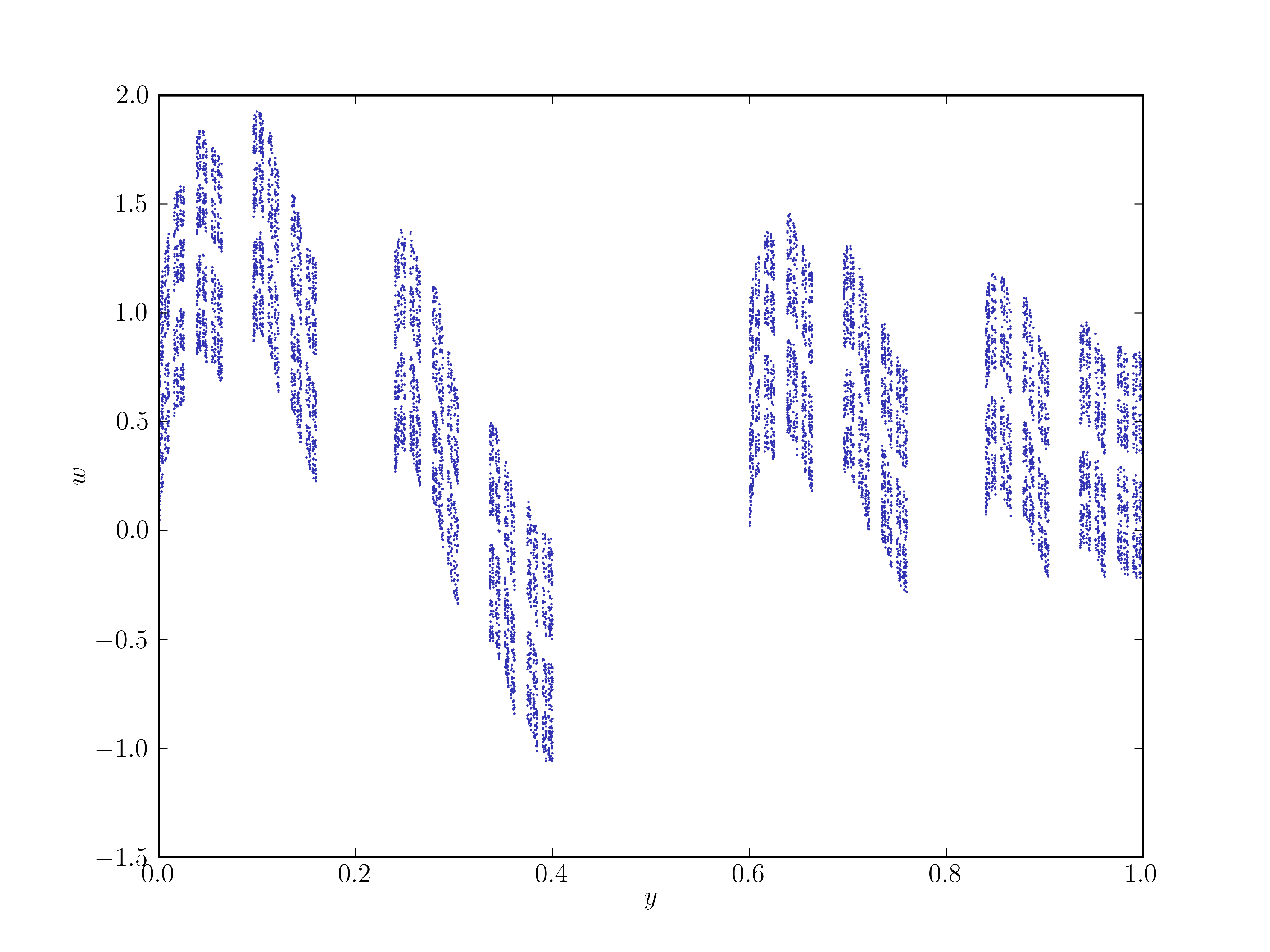
Figure 1: Plot of the intersection of the 4-dimensional attractor of the uni-directionally coupled system for $\alpha=0.4$, $\beta=0.43$ and $g(x,y)=\cos\big{(}\frac{\pi}{2}x\big{)}\sin\big{(}\frac{3\pi}{2}y\big{)}$ with the $w$-$y$ plane for fixed $x$ and $z$. Different values of $x$ and $z$ give similar cross-sections. Topologically, the attractor is the product of a Cantor dust-like set, as shown in the figure above, and the unit square.

With Figure 1 the reader can get an impression of what the attractor of the uni-directional coupled system can look like. The main task will be to determine the dimension of the physical measure that is supported on this attractor.

The outline of this article is as follows. In the next section, we recall the main notions that are necessary to state the properties of the coupled system. We also restate the Kaplan-Yorke conjecture more precisely, adjusted to our setting. In the third section, we will prove all the assertions (in particular, Corollary 3.7 and Theorem 3.11) that are needed in order verify Theorem 1.1. We conclude the article with a discussion of our results, their implications for more general systems, and related work on the dimensionality of filtered chaotic signals.

Acknowledgments. The majority of this work was carried out while the first author was undertaking a Fulbright scholarship at the University of Maryland, College Park. Also, the first author was partially funded by an Emmy-Noether-grant of the German Research Council (DFG-grant JA 1721/2-1). The authors are grateful to Daniel Karrasch and Markus Waurick for many helpful and enlightening discussions. This work is related to the activities of the Scientific Network “Skew product dynamics and multifractal analysis” (DFG grant OE 538/3-1).

2 Preliminaries

In the following, we will denote by $\mathcal{B}(M)$ the Borel $\sigma$-algebra of a subset $M\subseteq\mathbb{R}^{d}$ and with $\lambda^{d}$ the Lebesgue measure on $\mathbb{R}^{d}$. Further, $\mathring{M}$ will denote the interior of $M$ and $\overline{M}$ the closure of $M$.

Definition 2.1.

Let $F:M\subseteq\mathbb{R}^{d}\to M$ be a map with $M$ locally compact and assume there exist finitely many pairwise disjoint connected subsets $U_{i}\in\mathcal{B}\big{(}M\big{)}$ such that

$$M=\bigcup\limits_{i}U_{i}$$

and the map $\left.F\right|_{U_{i}}$ is continuous for each $U_{i}$ (with respect to the relative topology) plus $\left.F\right|_{\mathring{U_{i}}}$ is $C^{1}$. Furthermore, we assume that

$$\max_{i}\left\|\left.(F\right|_{\mathring{U_{i}}})^{\prime}\right\|_{\infty}<\infty$$

and $\lambda^{d}(M_{0})=0$ with

$$M_{0}:=\bigcup\limits_{n\in\mathbb{N}_{0}}F^{-n}\left(M\backslash\bigcup\limits_{i}\mathring{U_{i}}\right).$$

Then, we call $F$ a piecewise $C^{1}$ dynamical system.

Note that a subset $M\subseteq\mathbb{R}^{d}$ is locally compact if and only if there exist an open subset $A\subseteq\mathbb{R}^{d}$ and a closed subset $B\subseteq\mathbb{R}^{d}$ such that $M=A\cap B$ [Dug89, Theorem 6.5]. This means in particular $M\in\mathcal{B}(\mathbb{R}^{d})$ and therefore $M_{0}\in\mathcal{B}(\mathbb{R}^{d})$. We require $\lambda^{d}(M_{0})=0$ to avoid that orbits could be mapped into an open subset where the derivative is not defined. Such an open subset could be considered as a hole and therefore could cause positive escape rates which in turn would involve a different definition of the Lyapunov dimension.

Definition 2.2.

Let $F:M\subseteq\mathbb{R}^{d}\to M$ be a piecewise $C^{1}$ dynamical system and let $\mu$ be an $F$-invariant Borel probability measure on $M$. We call $\mu$ a physical measure if there exists a set $V\subseteq M$ of positive Lebesgue measure such that for every bounded continuous function $\varphi:M\to\mathbb{R}$,

$$\lim\limits_{N\to\infty}\frac{1}{N}\sum\limits_{n=0}^{N-1}\varphi(F^{n}(x))=\int\varphi d\mu,$$ (2)

for every $x\in V$.

Now, we will define the Lyapunov dimension following [AY84].

Definition 2.3.

Let $F:M\subseteq\mathbb{R}^{d}\to M$ be a piecewise $C^{1}$ dynamical system. Assume that $F$ has an ergodic invariant measure $\mu$ with $\mu(M_{0})=0$. Let

$$\chi_{1}(\mu)\geq\chi_{2}(\mu)\geq\dots\geq\chi_{d}(\mu)$$

be the Lyapunov exponents and set

$$j:=\max\{i:\chi_{1}(\mu)+\dots+\chi_{i}(\mu)\geq 0\},$$

(respectively, $0$ if $\chi_{1}(\mu)<0$). We define the Lyapunov or Kaplan-Yorke dimension as

$$D_{L}(\mu):=\begin{cases}0&\textnormal{ if }j=0\\ j+\frac{\chi_{1}(\mu)+\dots+\chi_{j}(\mu)}{\left|\chi_{j+1}(\mu)\right|}&\textnormal{ if }1\leq j<d\\ d&\textnormal{ if }j=d\end{cases}.$$

Note that by the required assumptions in the last definition the existence of the Lyapunov exponents is ensured by Oseledets theorem. The Kaplan-Yorke conjecture is referring to this situation, see [FOY83] or [FKYY83]. In these references, one can also find a heuristic derivation and interpretation of the Lyapunov dimension. For more information on the Lyapunov exponents, see e.g. [BP02].

Before we can state the Kaplan-Yorke conjecture for our setting, we will define all the other dimensions that we need in this paper, following mainly [HK97]. From now on, let $\mu$ be a Borel probability measure supported on a bounded subset $A\subset\mathbb{R}^{d}$ and let $B(x,\varepsilon)\subset\mathbb{R}^{d}$ be an open ball around $x\in\mathbb{R}^{d}$ with radius $\varepsilon>0$.

Definition 2.4.

The lower and upper box-counting dimension of $A$ are defined as

$$\underline{D}_{B}(A):=\liminf\limits_{\varepsilon\to 0}\frac{\log N(A,\varepsilon)}{-\log\varepsilon},$$

$$\overline{D}_{B}(A):=\limsup\limits_{\varepsilon\to 0}\frac{\log N(A,\varepsilon)}{-\log\varepsilon},$$

where $N(A,\varepsilon)$ is the smallest number of balls of radius $\varepsilon$ that can cover $A$. If $\underline{D}_{B}(A)=\overline{D}_{B}(A)$, then their common value $D_{B}(A)$ is called the box-counting dimension of $A$.

Definition 2.5.

For each point $x$, we define the lower and upper pointwise dimension of $\mu$ at $x$ to be

$$\underline{d}(\mu,x):=\liminf\limits_{\varepsilon\to 0}\frac{\log\mu(B(x,\varepsilon))}{\log\varepsilon},$$

$$\overline{d}(\mu,x):=\limsup\limits_{\varepsilon\to 0}\frac{\log\mu(B(x,\varepsilon))}{\log\varepsilon}.$$

If $\underline{d}(\mu,x)=\overline{d}(\mu,x)$, then their common value $d(\mu,x)$ is called the pointwise dimension of $\mu$ at $x$. We say that the measure $\mu$ is exact dimensional if the pointwise dimension exists and is constant almost everywhere, i.e.

$$\underline{d}(\mu,x)=\overline{d}(\mu,x)=:d(\mu),$$

for $\mu$-almost every $x\in A$.

Proposition 2.6 ([Fal97, Proposition 10.3], [Fal03, Proposition 3.8]).

For $\mu$-almost every $x\in A$ we have

$$\overline{d}(\mu,x)\leq\overline{D}_{B}(A).$$

Definition 2.7.

The lower and upper information dimension of $\mu$ are defined as

$$\underline{D}_{1}(\mu):=\liminf\limits_{\varepsilon\to 0}\frac{\int\log\mu(B(x,\varepsilon))d\mu(x)}{\log\varepsilon},$$

$$\overline{D}_{1}(\mu):=\limsup\limits_{\varepsilon\to 0}\frac{\int\log\mu(B(x,\varepsilon))d\mu(x)}{\log\varepsilon}.$$

If $\underline{D}_{1}(\mu)=\overline{D}_{1}(\mu)$, then their common value $D_{1}(\mu)$ is called the information dimension of $\mu$.

Commonly, a grid based definition of the information dimension is used but for our setting the integral and grid based definition coincide, see [BGT01, Theorem 2.1].

Theorem 2.8 ([Cut91, Theorem 2.2],[MR07, Theorem 1]).

We have

$$\int\underline{d}(\mu,x)d\mu(x)\leq\underline{D}_{1}(\mu)\leq\overline{D}_{1}(\mu)\leq\int\overline{d}(\mu,x)d\mu(x).$$

That means, provided the pointwise dimension exists almost everywhere,

$$D_{1}(\mu)=\int d(\mu,x)d\mu(x),$$

i.e. we can interpret the information dimension of the measure $\mu$ as the averaged pointwise dimension of $\mu$. In particular, if $\mu$ is exact dimensional, then $D_{1}(\mu)=d(\mu)$. Note that in this case also several other dimensions of the measure coincide [You82].

Now, we can state the Kaplan-Yorke conjecture for our setting.

Conjecture 2.9.

Given a locally compact subset $M\subseteq\mathbb{R}^{d}$. For “typical” piecewise $C^{1}$ dynamical systems $F:M\to M$ with an ergodic invariant physical measure $\mu$, we have that

$$D_{1}(\mu)=D_{L}(\mu).$$

In [FKYY83] it is conjectured that in this context $\mu$ is exact dimensional with $d(\mu)=D_{L}(\mu)$ and therefore $D_{1}(\mu)=D_{L}(\mu)$. Indeed, our main result will be of this type.

As already mentioned in the introduction, the word “typical” is not precisely defined in the conjecture. Thereby, one problem is that in infinite dimensional vector spaces there is no natural notion of typical phenomena, in the sense of “Lebesgue almost everywhere”, respectively, “Lebesgue measure zero”. One way to define it is to use the topological notion based on the category theorem of Baire. Prevalence is another concept to provide an analog of what typical could mean in the context of infinite dimensional vector spaces. In our case, we are dealing with the space of $C^{1}$ maps where the map and the derivative are bounded. We refer to [OY05] and [HK10] for more general definitions and examples regarding the notion of prevalence.

Definition 2.10.

Let $V$ be a completely metrizable topological vector space. A Borel measure $\nu$ is said to be transverse to a Borel set $E^{\prime}\subset V$ if there exists a compact subset $S\subset V$ with $0<\nu(S)<\infty$ and $\nu(E^{\prime}+v)=0$ for all $v\in V$. A subset $E\subset V$ will be called shy if there exist a Borel set $E^{\prime}\subset V$ with $E\subseteq E^{\prime}$ and a measure $\nu$ that is transverse to $E^{\prime}\subset V$. The complement of a shy set is called a prevalent set.

Note that if this concept is applied to $V=\mathbb{R}^{d}$ the only transverse measure is Lebesgue measure. This motivates the following definition.

Definition 2.11.

A finite dimensional subspace $P\subset V$ will be called a probe for a set $T\subset V$ if Lebesgue measure supported on $P$ is transverse to a Borel set containing the complement of $T$.

One of our main tools will be the potential theoretic method for the pointwise dimension.

Definition 2.12.

For $s\geq 0$ define the $s$-potential of $\mu$ at a point $x\in\mathbb{R}^{d}$ as

$$\varphi_{s}(\mu,x):=\int\frac{1}{\left|x-y\right|^{s}}d\mu(y).$$

Theorem 2.13 ([SY97]).

For $x\in A$ we have

$$\underline{d}(\mu,x)=\sup\{s:\varphi_{s}(\mu,x)<\infty\}=\inf\{s:\varphi_{s}(\mu,x)=\infty\}.$$

3 Proofs

From now on, we assume

$$0<\alpha,\beta<\frac{1}{2}$$

and set

$$M:=[0,1)\times\mathbb{R}.$$

First, we define the 2-dimensional and the uncoupled skinny baker’s map.

Definition 3.1.

The (2-dimensional) skinny baker’s map is defined as

$$B_{\alpha}:M\subset\mathbb{R}^{2}\to M:(x,y)\mapsto\begin{cases}(2x,\alpha y)&\textnormal{ if }0\leq x<\frac{1}{2}\\ \\ (2x-1,\alpha y+1-\alpha)&\textnormal{ if }\frac{1}{2}\leq x<1\end{cases}.$$

The uncoupled skinny baker’s map is defined as

$$B:M^{2}\subset\mathbb{R}^{4}\to M^{2}:(x,y,z,w)\mapsto(B_{\alpha}(x,y),B_{\beta}(z,w)),$$

where $M^{2}=M\times M$.

We will state some basic facts of the 2-dimensional skinny baker’s map, for more details see [AY84] and [FOY83]. The attractor of $B_{\alpha}$ is just the product of the interval $[0,1)$ in the $x$-direction and a Cantor set (determined by the parameter $\alpha$ and denoted by $A_{\alpha}$ in the following) in the $y$-direction. The box-counting dimension of the attractor is $1-\frac{\log 2}{\log\alpha}$ (this also holds for the Hausdorff dimension of the attractor). The physical measure $\mu_{\alpha}$ of $B_{\alpha}$ is unique (the basin is Lebesgue almost every point) and it is the product of the Lebesgue measure in the $x$-direction and the Cantor measure in the $y$-direction, denoted by $\nu_{\alpha}$ in the following. Furthermore, $\mu_{\alpha}$ is strong-mixing and is exact dimensional with the same value as the box-counting dimension.

From these facts we can deduce some properties of the uncoupled skinny baker’s map. The product set $A:=[0,1)\times A_{\alpha}\times[0,1)\times A_{\beta}$ is invariant under $B$ and we will see in the first proposition that $A$ is also the attractor of $B$. Further, the product measure $\mu:=\mu_{\alpha}\times\mu_{\beta}$ is invariant under $B$ and is also strong-mixing [Bro76, Proposition 1.6], i.e. in particular ergodic. Later, we will see that it is the unique physical measure of the uncoupled system, too. Since the box-counting and Hausdorff dimension of the attractor of $B_{\alpha}$ coincide and since the pointwise dimension is additive, we have

$$D_{B}(A)=d(\mu)=2-\frac{\log 2}{\log\alpha}-\frac{\log 2}{\log\beta}.$$

Next, we will define the coupled skinny baker’s maps. In order to do this, we will need a space of coupling functions. For that purpose, consider an open subset $U\subseteq\mathbb{R}^{d}$ and denote by $C_{b}^{1}(U)$ the space of all $C^{1}$ maps $g:U\to\mathbb{R}$ where $g$ and $g^{\prime}$ are bounded. Note that $C_{b}^{1}(U)$ equipped with the norm $\left\|g\right\|_{1,\infty}:=\max\{\left\|g\right\|_{\infty},\left\|g^{\prime}\right\|_{\infty}\}$ is a Banach space, where $\left\|\cdot\right\|_{\infty}$ denotes the uniform norm. Also note that $\mathring{M}$ is convex and therefore $g\in C_{b}^{1}(\mathring{M})$ is Lipschitz continuous. Hence, $g$ has a unique continuous extension on $\overline{M}$ and therefore $g(0,y)$ with $y\in\mathbb{R}$ is well-defined (with the convention of using the same symbol for the extension). That is why, we will just write $g\in C_{b}^{1}(M)$ from now on.

Definition 3.2.

For $g\in C_{b}^{1}(M)$, we define the coupled skinny baker’s map as

$$B_{g}:M^{2}\subset\mathbb{R}^{4}\to M^{2}:(x,y,z,w)\mapsto(B_{\alpha}(x,y),B_{\beta}(z,w)+(0,g(x,y))).$$

The uncoupled and coupled skinny baker’s map are piecewise $C^{1}$ dynamical systems, where the domain $M^{2}$ has the partition

$$U_{1} :=\left[0,\frac{1}{2}\right)\times\mathbb{R}\times\left[0,\frac{1}{2}\right)\times\mathbb{R},\quad U_{2}:=\left[0,\frac{1}{2}\right)\times\mathbb{R}\times\left[\frac{1}{2},1\right)\times\mathbb{R},$$

$$U_{3} :=\left[\frac{1}{2},1\right)\times\mathbb{R}\times\left[\frac{1}{2},1\right)\times\mathbb{R},\quad U_{4}:=\left[\frac{1}{2},1\right)\times\mathbb{R}\times\left[0,\frac{1}{2}\right)\times\mathbb{R}$$

and

$$M^{2}_{0}=\{(x,y,z,w)\in M^{2}:x\textnormal{ or }z\textnormal{ is a dyadic fraction or }0\},$$

with $\lambda^{4}(M^{2}_{0})=0$. Furthermore, we have for the derivative (piecewise, i.e. on each $\mathring{U}_{i}$)

$$B_{g}^{\prime}(x,y,z,w)=\begin{pmatrix}2&0&0&0\\ 0&\alpha&0&0\\ 0&0&2&0\\ g_{x}(x,y)&g_{y}(x,y)&0&\beta\end{pmatrix}$$ (3)

and the derivative is (piecewise) bounded because $g\in C_{b}^{1}(M)$ (note that by $g_{x}$ we mean the partial derivative of $g$ with respect to the variable $x$).

A direct calculation gives that the Lyapunov exponents of the uncoupled skinny baker’s map are $\log 2$, $\log 2$, $\log\alpha$ and $\log\beta$ almost everywhere with respect to the Lebesgue measure and the physical measure. This implies for $\alpha\leq\beta$

$$D_{L}(\mu)=\begin{cases}2-2\frac{\log 2}{\log\beta}&\textnormal{ if }\beta\leq\frac{1}{4}\\ 3-2\frac{\log 2}{\log\alpha}-\frac{\log\beta}{\log\alpha}&\textnormal{ if }\beta\geq\frac{1}{4}\end{cases}$$

(for $\alpha\geq\beta$ interchange $\alpha$ with $\beta$). Observe that $d(\mu)=D_{1}(\mu)<D_{L}(\mu)$ for $\alpha\neq\beta$ and $d(\mu)=D_{1}(\mu)=D_{L}(\mu)$ for $\alpha=\beta$, i.e. the Kaplan-Yorke equality fails for Lebesgue almost every $(\alpha,\beta)\in\big{(}0,\frac{1}{2}\big{)}^{2}$.

In Figure 2, we show the information dimension and Lyapunov dimension of the uncoupled skinny baker’s map for fixed $\alpha=0.05$. Note the relation between the two branches of the Lyapunov dimension for $\beta\geq 0.05$.

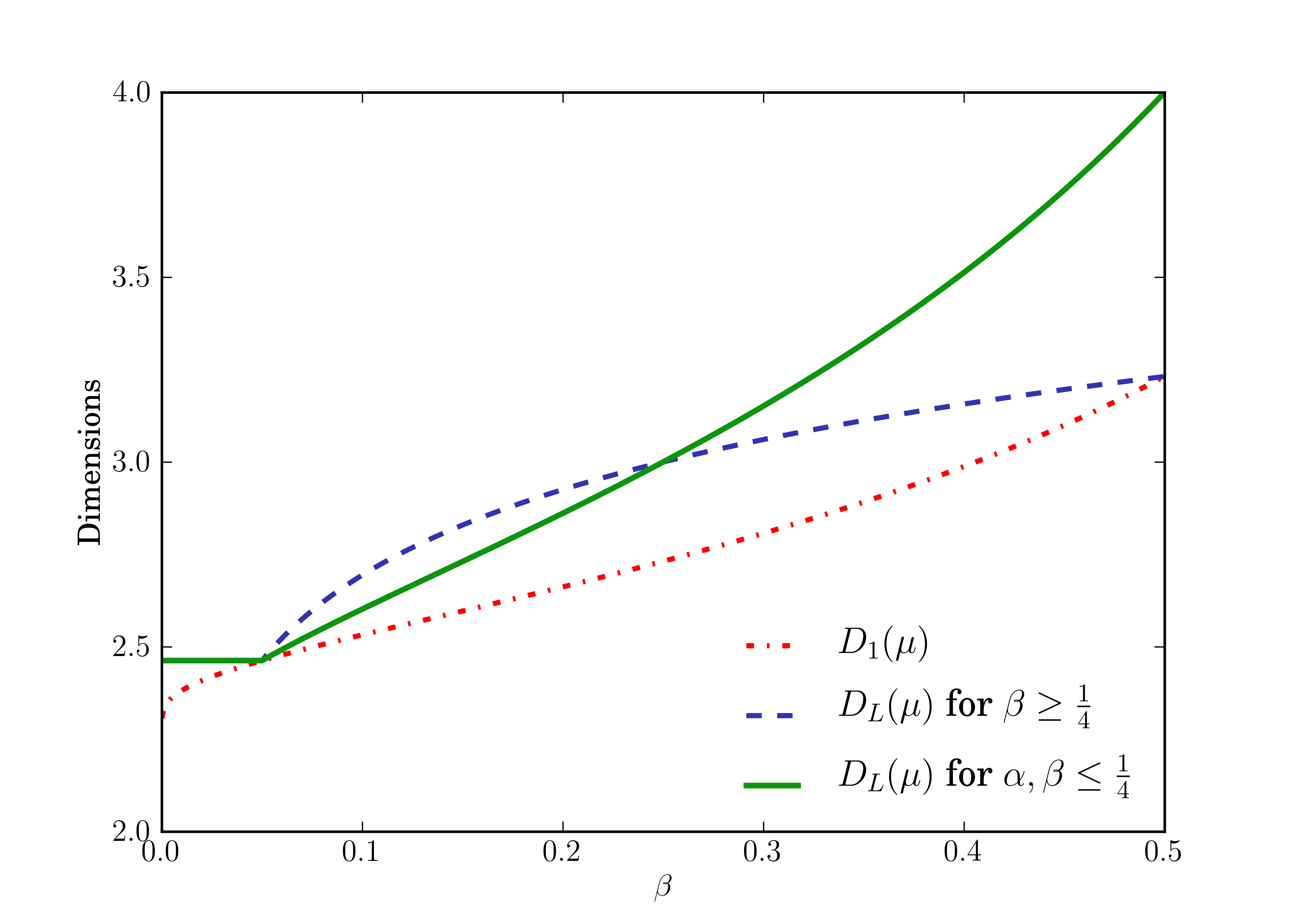
Figure 2: The information dimension $D_{1}(\mu)$ and the Lyapunov dimension $D_{L}(\mu)$ for the uncoupled skinny baker’s map for fixed $\alpha=0.05$.

Proposition 3.3.

For $g\in C_{b}^{1}(M)$, the attractor $A_{g}$ of the coupled skinny baker’s map is the image of a map ${h_{g}}$, where the domain of ${h_{g}}$ is the attractor of the uncoupled skinny baker’s map. The conjugacy ${h_{g}}:A\to A_{g}$ is defined as

$${h_{g}^{\pm 1}}(x,y,z,w):=\left(x,y,z,w\pm\sum_{i=0}^{\infty}\beta^{i}g\left(B_{\alpha}^{-i-1}(x,y)\right)\right).$$

We have $B(x,y,z,w)={h_{g}^{-1}}(B_{g}({h_{g}}(x,y,z,w)))$ and furthermore, for

1. $\alpha>\beta$: ${h_{g}}$ is bi-Lipschitz,

2. $\alpha=\beta$: ${h_{g}^{\pm 1}}$ is Hölder continuous for all Hölder exponents $\rho<1$,

3. $\alpha<\beta$: ${h_{g}}$ is Hölder continuous with Hölder exponent $\rho=\frac{\log\beta}{\log\alpha}$.

Proof.

For $a\in[0,1]$ let $((a)_{i})_{i\in\mathbb{N}_{0}}$ be the binary representation of $a$ with $(a)_{i}$ zero or one for all $i\in\mathbb{N}_{0}$ and

$$a=\sum\limits_{i=0}^{\infty}\frac{(a)_{i}}{2^{i+1}}.$$

In the case that $a$ is a dyadic fraction, we have to make a choice between the terminating or non-terminating representation to ensure the uniqueness of the binary representation. For $n\in\mathbb{N}_{0}$ and $(x,y,w,z)\in M^{2}$, define

$$(x_{n},y_{n},z_{n},w_{n}):=B_{g}^{n}(x,y,z,w)$$ (4)

and a direct calculation shows

$$x_{n} =2^{n}x-\sum\limits_{i=0}^{n-1}2^{n-1-i}(x)_{i},\quad y_{n}=\alpha^{n}y+(1-\alpha)\sum\limits_{i=0}^{n-1}\alpha^{n-1-i}(x)_{i},$$

$$z_{n} =2^{n}z-\sum\limits_{i=0}^{n-1}2^{n-1-i}(z)_{i},\quad w_{n}=\beta^{n}w+(1-\beta)\sum\limits_{i=0}^{n-1}\beta^{n-1-i}(z)_{i}+\sum\limits_{i=0}^{n-1}\beta^{n-1-i}g(x_{i},y_{i}).$$

First, we want to explain that the series in the definition of ${h_{g}}$ is well-defined: for $B_{\alpha}$ restricted to $[0,1)\times[0,1]$ we can define an inverse map by

$$B_{\alpha}^{-1}(x,y):=\begin{cases}\left(\frac{x}{2},\frac{y}{\alpha}\right)&\textnormal{ if }y\leq\frac{1}{2}\\ \\ \left(\frac{x+1}{2},\frac{y-(1-\alpha)}{\alpha}\right)&\textnormal{ if }y>\frac{1}{2}\end{cases},$$

on $[0,1)\times([0,\alpha]\cup[1-\alpha,1])$. Since $[0,1)\times A_{\alpha}$ is the attractor of $B_{\alpha}$, we have

$$(x,y) \in[0,1)\times A_{\alpha}=B_{\alpha}([0,1)\times A_{\alpha})$$

$$\Longleftrightarrow(x,y)\in[0,1)\times A_{\alpha},B_{\alpha}([0,1)\times A_{\alpha}),B_{\alpha}^{2}([0,1)\times A_{\alpha}),\ldots$$

and this means

$$\ldots,B_{\alpha}^{-2}(x,y),B_{\alpha}^{-1}(x,y),(x,y)\in[0,1)\times A_{\alpha},$$

i.e. each $(x,y)\in[0,1)\times A_{\alpha}$ has a unique infinite past history

$$(x_{-n},y_{-n}):=B_{\alpha}^{-n}(x,y),$$ (5)

with $n\in\mathbb{N}$ on the attractor. Thus, for $(x,y)\in[0,1)\times A_{\alpha}$ the occurring series in ${h_{g}}$ is well-posed and convergent, since $g$ is bounded. Furthermore, for each $n\in\mathbb{N}$

$$y=\alpha^{n}y_{-n}+(1-\alpha)\sum_{j=0}^{n-1}\alpha^{j}(x_{-j-1})_{0},$$

where $j=n-1-i$ and $(x_{-n})_{n-1-j}=(x_{-j-1})_{0}$. Therefore, in the limit,

$$y=(1-\alpha)\sum_{i=0}^{\infty}\alpha^{i}(x_{-i-1})_{0}$$

and we have the analog result for $(z,w)\in[0,1)\times A_{\beta}$ (for the uncoupled system). We will need this result and a similar argument to show that ${h_{g}}(A)$ is the attractor for the coupled skinny baker’s map: direct computation gives for $(x,y,z,w)\in[0,1)\times A_{\alpha}\times M$

$${h_{g}}((B(x,y,z,w))=B_{g}({h_{g}}(x,y,z,w))$$ (6)

and we will see that only $(x,y,z,w)\in A$ matter. For some $\delta>0$, define the set

$$V:=[0,1)\times[-\delta,1+\delta]\times[0,1)\times\left[-\delta-\frac{\left\|g\right\|_{\infty}}{1-\beta},1+\delta+\frac{\left\|g\right\|_{\infty}}{1-\beta}\right].$$

Note that $B_{g}(V)\subset V$, i.e. we can define

$$A_{g}:=\bigcap\limits_{n\in\mathbb{N}}B_{g}^{n}(V).$$

Also note that ${h_{g}}(A)\subset V$ and due to (6), we have ${h_{g}}(A)=B_{g}^{n}({h_{g}}(A))\subset B_{g}^{n}(V)$ for each $n\in\mathbb{N}$, i.e. ${h_{g}}(A)\subset A_{g}$. Now, using a similar argument as above, we will show ${h_{g}}(A)=A_{g}$. We have that each $(x,y,z,\tilde{w})\in A_{g}$ has at least one past history, denoted by $(x_{-1},y_{-1},z_{-1},\tilde{w}_{-1})$ and this point has also at least one past history, denoted by $(x_{-2},y_{-2},z_{-2},\tilde{w}_{-2})$ and so on. Every single possible, infinite past history is a subset of $V$, i.e. is bounded. For each $n\in\mathbb{N}$ we have

$$\tilde{w}=\beta^{n}\tilde{w}_{-n}+(1-\beta)\sum_{j=0}^{n-1}\beta^{j}(z_{-j-1})_{0}+\sum_{j=0}^{n-1}\beta^{j}g\left(x_{-j-1},y_{-i-1}\right),$$

again $j=n-1-i$ and $(z_{-n})_{n-1-j}=(z_{-j-1})_{0}$. Thus, in the limit,

$$\tilde{w}=(1-\beta)\sum_{i=0}^{\infty}\beta^{i}(z_{-i-1})_{0}+\sum_{i=0}^{\infty}\beta^{i}g\left(B_{\alpha}^{-i-1}(x,y)\right)=w+\sum_{i=0}^{\infty}\beta^{i}g\left(B_{\alpha}^{-i-1}(x,y)\right),$$

with $(x,y,z,w)\in A$. This shows ${h_{g}}(A)=A_{g}$. It also follows that ${h_{g}}$ is injective, i.e. the inverse map ${h_{g}^{-1}}:A_{g}\to A$ exists and is given as stated above.

Now, we prove the continuity properties of ${h_{g}}$. Let $(x,y,z,w),(\tilde{x},\tilde{y},\tilde{z},\tilde{w})\in A$ and

$$\left\|{h_{g}}(x,y,z,w)-{h_{g}}(\tilde{x},\tilde{y},\tilde{z},\tilde{w})\right\| =\left\|(x-\tilde{x},y-\tilde{y},z-\tilde{z},w-\tilde{w}+\Delta_{g})\right\|$$

$$\leq\left|x-\tilde{x}\right|+\left|y-\tilde{y}\right|+\left|z-\tilde{z}\right|+\left|w-\tilde{w}\right|+\left|\Delta_{g}\right|,$$

with

$$\Delta_{g}=\sum_{i=0}^{\infty}\beta^{i}\left[g\left(B_{\alpha}^{-i-1}(x,y)\right)-g\left(B_{\alpha}^{-i-1}(\tilde{x},\tilde{y})\right)\right].$$

The estimation of $\Delta_{g}$ will be the main task. First, note that

$$\left|\Delta_{g}\right|\leq\mathrm{Lip}(g)\sum_{i=0}^{\infty}\beta^{i}\left\|B_{\alpha}^{-i-1}(x,y)-B_{\alpha}^{-i-1}(\tilde{x},\tilde{y})\right\|.$$ (7)

For $y=\tilde{y}$,

$$\left\|B_{\alpha}^{-i-1}(x,y)-B_{\alpha}^{-i-1}(\tilde{x},\tilde{y})\right\|\leq\left|x-\tilde{x}\right|$$

because

$$B_{\alpha}^{-i-1}(x,y)=\left(x_{-i-1},y_{-i-1}\right)=\left(\frac{x_{-i}+(y_{-i})_{0}}{2},\frac{y_{-i}-(1-\alpha)(y_{-i})_{0}}{\alpha}\right),$$

and therefore

$$y_{-i-1}-\tilde{y}_{-i-1}=0\quad\textrm{ and }\quad x_{-i-1}-\tilde{x}_{-i-1}=\frac{x-\tilde{x}}{2^{i+1}}.$$

For $\left|y-\tilde{y}\right|\geq(1-2\alpha)$, we have

$$\left\|B_{\alpha}^{-i-1}(x,y)-B_{\alpha}^{-i-1}(\tilde{x},\tilde{y})\right\|<2\leq\frac{2}{1-2\alpha}\left|y-\tilde{y}\right|.$$

That means, for this two cases,

$$\left|\Delta_{g}\right|\leq\frac{\mathrm{Lip}(g)}{1-\beta}\left[\left|x-\tilde{x}\right|+\frac{2}{1-2\alpha}\left|y-\tilde{y}\right|\right].$$

To handle the remaining case, consider for each $k\in\mathbb{N}_{0}$

$$(1-2\alpha)\alpha^{k}>\left|y-\tilde{y}\right|\geq(1-2\alpha)\alpha^{k+1}.$$ (8)

If $y$ and $\tilde{y}$ satisfy this condition for a $k\in\mathbb{N}_{0}$, then they stay close together (in the sense that they are both in $[0,\alpha]$ or in $[1-\alpha,1]$) for $k$ steps backward and we can split the sum in (7) into the first $k$ parts and the remaining part. We get the following upper bound

$$\frac{\left|\Delta_{g}\right|}{\mathrm{Lip}(g)}\leq\sum\limits_{i=0}^{k}\frac{\beta^{i}}{2^{i+1}}\left|x-\tilde{x}\right|+\sum\limits_{i=0}^{k}\frac{\beta^{i}}{\alpha^{i+1}}\left|y-\tilde{y}\right|+\frac{2}{1-\beta}\beta^{k+1}.$$ (9)

The factor in front of $\left|x-\tilde{x}\right|$ is smaller than $\frac{1}{2-\beta}<\frac{1}{1-\beta}$, independent of $k$ and the relation between $\alpha$ and $\beta$.

For $\alpha>\beta$ we can get $k$-independent estimates for the other two terms in (9),

$$\sum\limits_{i=0}^{k}\frac{\beta^{i}}{\alpha^{i+1}}\left|y-\tilde{y}\right|\leq\frac{1}{\alpha-\beta}\left|y-\tilde{y}\right|\quad\textrm{ and }\quad\frac{2}{1-\beta}\beta^{k+1}\leq\frac{2}{(1-\beta)(1-2\alpha)}\left|y-\tilde{y}\right|,$$

where we used (8) for the third term. Hence, for all $(x,y,z,w),(\tilde{x},\tilde{y},\tilde{z},\tilde{w})\in A$

$$\left\|{h_{g}}(x,y,z,w)-{h_{g}}(\tilde{x},\tilde{y},\tilde{z},\tilde{w})\right\|\leq \left[1+\frac{\mathrm{Lip}(g)}{1-\beta}\right]\left|x-\tilde{x}\right|$$

$$+ \left[1+\mathrm{Lip}(g)\left[\frac{1}{\alpha-\beta}+\frac{2}{(1-\beta)(1-2\alpha)}\right]\right]\left|y-\tilde{y}\right|$$

$$+ \left|z-\tilde{z}\right|+\left|w-\tilde{w}\right|.$$

The same result applies to ${h_{g}^{-1}}$, i.e. ${h_{g}}$ is bi-Lipschitz for $\alpha>\beta$.

For $\alpha=\beta$, using (8), the second term in (9) is bounded above by

$$\sum\limits_{i=0}^{k}\frac{\beta^{i}}{\alpha^{i+1}}\left|y-\tilde{y}\right|=\frac{k+1}{\alpha}\left|y-\tilde{y}\right|<\frac{1}{\alpha}\left|y-\tilde{y}\right|+\frac{1}{\alpha\log\alpha}\left|y-\tilde{y}\right|\log\left|y-\tilde{y}\right|.$$

For $\rho\in[0,1)$ we can always find a constant $C(\rho)>0$ such that

$$-\left|y-\tilde{y}\right|^{1-\rho}\log\left|y-\tilde{y}\right|\leq C(\rho),$$

i.e. for all $(x,y,z,w),(\tilde{x},\tilde{y},\tilde{z},\tilde{w})\in A$

$$\left\|{h_{g}}(x,y,z,w)-{h_{g}}(\tilde{x},\tilde{y},\tilde{z},\tilde{w})\right\|\leq \left[1+\frac{\mathrm{Lip}(g)}{1-\alpha}\right]\left|x-\tilde{x}\right|$$

$$+ \left[1+\frac{\mathrm{Lip}(g)}{\alpha}\left[1-\frac{C(\rho)}{\log\alpha}+\frac{2}{(1-\alpha)(1-2\alpha)}\right]\right]\left|y-\tilde{y}\right|^{\rho}$$

$$+ \left|z-\tilde{z}\right|+\left|w-\tilde{w}\right|.$$

Again, the same result applies to ${h_{g}^{-1}}$, i.e. ${h_{g}}$ and ${h_{g}^{-1}}$ are Hölder continuous for all Hölder exponents $\rho<1$ for $\alpha=\beta$.

The last case is $\alpha<\beta$. Set

$$\rho:=\frac{\log\beta}{\log\alpha}.$$

We observe first that (8) is equivalent to

$$(1-2\alpha)^{\rho}\beta^{k}>\left|y-\tilde{y}\right|^{\rho}\geq(1-2\alpha)^{\rho}\beta^{k+1}$$ (10)

and therefore

$$\left(\frac{\beta}{\alpha}\right)^{k+1}\left|y-\tilde{y}\right|\leq\frac{(1-2\alpha)^{1-\rho}}{\alpha}\left|y-\tilde{y}\right|^{\rho}.$$

Furthermore, by using the relation

$$\sum\limits_{i=0}^{k}q^{k}=\frac{q^{k+1}-1}{q-1},$$

for $q\neq 1$, we get

$$\sum\limits_{i=0}^{k}\frac{\beta^{i}}{\alpha^{i+1}}\left|y-\tilde{y}\right|<\frac{1}{\beta-\alpha}\left(\frac{\beta}{\alpha}\right)^{k+1}\left|y-\tilde{y}\right|\leq\frac{(1-2\alpha)^{1-\rho}}{\alpha(\beta-\alpha)}\left|y-\tilde{y}\right|^{\rho}.$$

Hence, using (10) for the last term in (9), for all $(x,y,z,w),(\tilde{x},\tilde{y},\tilde{z},\tilde{w})\in A$

$$\left\|{h_{g}}(x,y,z,w)-{h_{g}}(\tilde{x},\tilde{y},\tilde{z},\tilde{w})\right\|\leq \left[1+\frac{\mathrm{Lip}(g)}{1-\beta}\right]\left|x-\tilde{x}\right|$$

$$+ \left[1+\frac{\mathrm{Lip}(g)}{(1-2\alpha)^{\rho}}\left[\frac{1}{\alpha(\beta-\alpha)}+\frac{2}{(1-\beta)(1-2\alpha)}\right]\right]\left|y-\tilde{y}\right|^{\rho}$$

$$+ \left|z-\tilde{z}\right|+\left|w-\tilde{w}\right|$$

(note that $(1-2\alpha)^{1-\rho}\leq(1-2\alpha)^{-\rho}$). ∎

There are two direct consequences of this proposition. The first one pinpoints the physical measure ${\mu_{g}}$ of the coupled skinny baker’s map. With the conjugacy ${h_{g}}$ we have a natural candidate, namely, the image measure of $\mu=\mu_{\alpha}\times\mu_{\beta}$. The second consequence is that for $\alpha\geq\beta$ all the dimensions of the attractor and the physical measure of the coupled and uncoupled system coincide.

Lemma 3.4.

For $g\in C_{b}^{1}(M)$ the image measure ${h_{g}}(\mu)=:{\mu_{g}}$ is invariant under $B_{g}$ and is ergodic. It is the unique physical measure of $B_{g}$, too.

Proof.

Since ${h_{g}}$ is a conjugacy on the support of $\mu$, it follows that ${\mu_{g}}$ is invariant under $B_{g}$ and ergodic. Now, we want to prove that ${\mu_{g}}$ is the unique physical measure. We will show that (2) holds for Lebesgue almost every point. It is enough to prove (2) for all continuous functions with compact support [Bau92, Theorem 29.12 and Corollary 30.9]. Using [Wal82, Lemma 6.13] and [Bau92, Lemma 31.4], we can find a set $W\in\mathcal{B}\big{(}M^{2}\big{)}$ with ${\mu_{g}}(W)=1$ such that for all $(x,y,z,w)\in W$ and for every continuous function $\varphi:M^{2}\to\mathbb{R}$ with compact support,

$$\lim\limits_{N\to\infty}\frac{1}{N}\sum\limits_{n=0}^{N-1}\varphi(B_{g}^{n}(x,y,z,w))=\int\varphi d{\mu_{g}}.$$ (11)

Furthermore, for $(x,y,z,w),(x,\tilde{y},z,\tilde{w})\in M^{2}$ we have

$$\lim\limits_{n\to\infty}\left\|B_{g}^{n}(x,y,z,w)-B_{g}^{n}(x,\tilde{y},z,\tilde{w})\right\|=0$$

because (using the notation (4) from the previous proof)

$$\left|y_{n}-\tilde{y}_{n}\right|=\alpha^{n}\left|y-\tilde{y}\right|$$

and

$$\left|w_{n}-\tilde{w}_{n}\right|\leq\beta^{n}\left|w-\tilde{w}\right|+\mathrm{Lip}(g)\left|y-\tilde{y}\right|\cdot\begin{cases}\frac{\alpha^{n}}{\alpha-\beta}&\textnormal{ if }\alpha>\beta\\ \alpha^{n-1}n&\textnormal{ if }\alpha=\beta\\ \frac{\beta^{n}}{\beta-\alpha}&\textnormal{ if }\alpha<\beta\end{cases}.$$

Therefore, we have for every continuous function $\varphi$ with compact support

$$\lim\limits_{n\to\infty}\left|\varphi(B_{g}^{n}(x,y,z,w))-\varphi(B_{g}^{n}(x,\tilde{y},z,\tilde{w}))\right|=0,$$

since $\varphi$ is also uniformly continuous. Hence, by using the Cesàro mean, we get

$$\lim\limits_{N\to\infty}\left|\frac{1}{N}\sum\limits_{n=0}^{N-1}\left[\varphi(B_{g}^{n}(x,y,z,w))-\varphi(B_{g}^{n}(x,\tilde{y},z,\tilde{w}))\right]\right|=0.$$

This means condition (11) is fulfilled for all $(x,y,z,w)\in M^{2}$ with $(x,z)\in\pi_{x,z}(W)$, where $\pi_{x,z}$ is the canonical projection onto $[0,1)^{2}\subset\mathbb{R}^{2}$. Note that $\pi_{x,z}(W)$ is Lebesgue measurable [KP08, Theorem 1.7.19 and Theorem 1.7.9]. Furthermore,

$$1 ={\mu_{g}}(W)\leq\mu(\{(x,y,z,w)\in([0,1)\times[0,1])^{2}:(x,z)\in\pi_{x,z}(W)\})$$

$$=\lambda^{2}(\pi_{x,z}(W))\nu_{\alpha}([0,1])\nu_{\beta}([0,1])=\lambda^{2}(\pi_{x,z}(W))\leq 1,$$

i.e. $\pi_{x,z}(W)$ has full measure in $[0,1)^{2}$. This and the property that $\lambda^{4}$ is $\sigma$-finite implies that the set of exceptions of (11) has zero measure. Therefore, for every continuous function $\varphi:M^{2}\to\mathbb{R}$ with compact support,

$$\lim\limits_{N\to\infty}\frac{1}{N}\sum\limits_{n=0}^{N-1}\varphi(B_{g}^{n}(x,y,z,w))=\int\varphi d{\mu_{g}},$$

for almost every $(x,y,z,w)\in M^{2}$ with respect to the Lebesgue measure. ∎

Since the uncoupled case corresponds to $g=0$, we also get that $\mu=\mu_{\alpha}\times\mu_{\beta}$ is the unique physical measure for the uncoupled skinny baker’s map $B$.

The second consequence of Proposition 3.3 follows directly for $\alpha>\beta$ from the bi-Lipschitz continuity of the conjugacy and for $\alpha=\beta$ from the Hölder continuity of the conjugacy and its inverse with arbitrary Hölder exponent $\rho<1$.

Corollary 3.5.

For $\alpha\geq\beta$ and $g\in C_{b}^{1}(M)$ we have that ${\mu_{g}}$ is exact dimensional with $d({\mu_{g}})=D_{1}({\mu_{g}})=d(\mu)$. We get $D_{B}(A_{g})=D_{B}(A)$, too (note that also other dimensions of the the physical measure and the attractor coincide).

Now, we calculate the Lyapunov exponents of the coupled skinny baker’s map.

Lemma 3.6.

For $g\in C_{b}^{1}(M)$ the Lyapunov exponents of the coupled skinny baker’s map $B_{g}$ are $\log 2$, $\log 2$, $\log\alpha$ and $\log\beta$ almost everywhere with respect to the Lebesgue measure and the physical measure.

Proof.

We consider points $(x,y,z,w)\in M^{2}\backslash M^{2}_{0}$. We have $\lambda^{4}(M^{2}_{0})=0$ and ${\mu_{g}}(M^{2}_{0})=0$, too. To compute directly the Lyapunov exponents at a point we have to find lower and upper bounds for $\left\|(B_{g}^{n})^{\prime}(x,y,z,w)v\right\|$ with $v\in\mathbb{R}^{4}$. The derivative $(B_{g}^{n})^{\prime}$ for all $n\in\mathbb{N}$ is given by

$$(B_{g}^{n})^{\prime}(x,y,z,w)=\prod\limits_{k=1}^{n}B_{g}^{\prime}({B_{g}^{n-k}(x,y,z,w)}).$$

Using (3), we get

$$(B_{g}^{n})^{\prime}(x,y,z,w)=\begin{pmatrix}2^{n}&0&0&0\\ 0&\alpha^{n}&0&0\\ 0&0&2^{n}&0\\ a_{n}(x,y)&b_{n}(x,y)&0&\beta^{n}\end{pmatrix},$$

with

$$a_{n}(x,y)=\sum\limits_{i=0}^{n-1}2^{i}\beta^{n-1-i}g_{x}(B_{\alpha}^{i}(x,y))\quad\textnormal{ and }\quad b_{n}(x,y)=\sum\limits_{i=0}^{n-1}\alpha^{i}\beta^{n-1-i}g_{y}(B_{\alpha}^{i}(x,y)).$$

Observe that $\log 2$ is a Lyapunov exponent with at least multiplicity 2. This is true because

$$\left\|(B_{g}^{n})^{\prime}(x,y,z,w)v\right\|^{2}=2^{2n}+(a_{n}(x,y)\cdot c)^{2}\leq(1+\left\|g_{x}\right\|_{\infty}^{2}c^{2})2^{2n}$$

for all $v=(c,0,d,0)$, $\left\|v\right\|=1$. We get the Lyapunov exponent $\log\beta$ for $v=(0,0,0,1)$. For $\alpha\geq\beta$ and $v=(0,1,0,0)$ we get the last Lyapunov exponent $\log\alpha$ because

$$\left|b_{n}(x,y)\right|\leq\left\|g_{y}\right\|_{\infty}\alpha^{n-1}\begin{cases}\frac{\alpha}{\alpha-\beta}&\textnormal{ if }\alpha>\beta\\ n&\textnormal{ if }\alpha=\beta\end{cases}$$

(for $\alpha=\beta$ we have for all $v=(0,c,0,d)$, $\left\|v\right\|=1$, $c\neq 0$ that $\left\|(B_{g}^{n})^{\prime}(x,y,z,w)v\right\|>\alpha^{n}\left|c\right|$ and therefore $\log\alpha$ has multiplicity 2). For $\alpha<\beta$ set $b_{\infty}(x,y):=\lim\limits_{n\to\infty}b_{n}(x,y)/\beta^{n}$ and use $v=(0,1,0,-b_{\infty}(x,y))$. Again, we get $\log\alpha$ because

$$\left|b_{n}(x,y)-\beta^{n}b_{\infty}(x,y)\right|\leq\frac{\left\|g_{y}\right\|_{\infty}}{\beta-\alpha}\alpha^{n}.$$

All this together proves the assertion. ∎

Note that the $w$-direction corresponds to the smallest Lyapunov exponent for $\alpha>\beta$, but not for $\alpha<\beta$.

Corollary 3.7.

The Lyapunov dimension of the coupled system coincides with the Lyapunov dimension of the uncoupled system for every $g\in C_{b}^{1}(M)$, i.e.

$$D_{L}({\mu_{g}})=D_{L}(\mu)=:D_{L}.$$

This implies for $\alpha\geq\beta$ that the relation between the information dimension and Lyapunov dimension of the coupled system is the same as for the uncoupled system, i.e $D_{1}({\mu_{g}})<D_{L}$ for $\alpha>\beta$ and $D_{1}({\mu_{g}})=D_{L}$ for $\alpha=\beta$.

Now, what is left is the case $\alpha<\beta$. With the next 4 assertions we will prove that $d({\mu_{g}})=D_{1}({\mu_{g}})=D_{L}$ in a prevalent sense, where we will mainly use the potential theoretic method for the pointwise dimension, see Theorem 2.13. The main step will be to establish a lower bound for the pointwise dimension, and in order to this we will show that for a prevalent set of $g$’s the following is true: for all $0\leq s<D_{L}$, the $s$-potential $\varphi_{s}({\mu_{g}},v)$ is finite for ${\mu_{g}}$ - a.e. $v$ in the attractor $A_{g}$ (defined in Proposition 3.3). The corresponding set of exceptions is

$$E:=\{g\in C_{b}^{1}(M):\textnormal{ there are }0\leq s<D_{L}\textnormal{ and }\\ W\subset A_{g}\textnormal{ with }{\mu_{g}}(W)>0\textnormal{ such that }\varphi_{s}({\mu_{g}},v)=\infty\textnormal{ for all }v\in W\}.$$ (12)

In Theorem 3.11 we will embed $E$ into a bigger Borel set and we will show that Lebesgue measure supported on the finite dimensional subspace

$$P:=\{(x,y)\mapsto\lambda\cdot p(x,y):\lambda\in\mathbb{R}\}\subset C_{b}^{1}(M)$$ (13)

is transverse to this bigger set, where we require $p(x,y)=y$ for all $(x,y)\in[0,1)\times[0,1]$.

Before we proceed, we want to motivate why we are choosing this prevalent setting. To use Theorem 2.13, we have to estimate

$$\varphi_{s}({\mu_{g}},v)=\int\limits_{A_{g}}\frac{1}{\left|v-\tilde{v}\right|^{s}}d{\mu_{g}}(\tilde{v}) =\int\limits_{A}\frac{1}{\left|{h_{g}}(x,y,z,w)-{h_{g}}(\tilde{x},\tilde{y},\tilde{z},\tilde{w})\right|^{s}}d\mu(\tilde{x},\tilde{y},\tilde{z},\tilde{w})$$

$$=\int\limits_{A}\frac{1}{(I^{2}+I_{g}^{2})^{s/2}}d\mu(\tilde{x},\tilde{y},\tilde{z},\tilde{w}),$$

for $v\in A_{g}$, $(x,y,z,w)={h_{g}^{-1}}(v)$ and with

$$I^{2} :=(x-\tilde{x})^{2}+(y-\tilde{y})^{2}+(z-\tilde{z})^{2},$$

$$I_{g} :=w-\tilde{w}+\sum_{i=0}^{\infty}\beta^{i}\left[g\left(B_{\alpha}^{-i-1}(x,y)\right)-g\left(B_{\alpha}^{-i-1}(\tilde{x},\tilde{y})\right)\right].$$

It is very difficult to estimate this integral for an arbitrary $g\in C_{b}^{1}(M)$. The notion of prevalence comes here into play, namely, by adding a linear perturbation term to $g$,

$$g_{\lambda}(x,y):=g(x,y)+\lambda\cdot p(x,y),$$

for $\lambda\in\mathbb{R}$ and estimating the following integral

$$\int\limits_{-\lambda_{0}}^{\lambda_{0}}\varphi_{s}({\mu_{g}}_{\!\scriptscriptstyle\lambda},{h_{g}}_{\!\scriptscriptstyle\lambda}(v))d\lambda =\int\limits_{-\lambda_{0}}^{\lambda_{0}}\;\int\limits_{A}\frac{1}{(I^{2}+(I_{g}+\lambda I_{p})^{2})^{s/2}}d\mu(\tilde{x},\tilde{y},\tilde{z},\tilde{w})d\lambda,$$ (14)

for $v=(x,y,z,w)\in A$ and (using the notation (5) from the proof of Proposition 3.3)

$$I_{p}:=\sum_{i=0}^{\infty}\beta^{i}\left[y_{-i-1}-\tilde{y}_{-i-1}\right].$$

Now, the main ingredient is to use Tonelli’s theorem. As a result, the order of integration in (14) can be interchanged and the estimation of the inner integral over $\lambda$ is feasible.

The next proposition will be the major technical step in the proof of Theorem 3.11. But first, we need the following lemma.

Lemma 3.8.

Assume $\alpha<\beta$. For sufficient small $\left|y-\tilde{y}\right|$ with $y,\tilde{y}\in A_{\alpha}$ we have that $I_{p}$ is bounded from above and below,

$$K_{1}\left|y-\tilde{y}\right|^{\rho}\geq\left|I_{p}\right|\geq K_{2}\left|y-\tilde{y}\right|^{\rho},$$

with $\rho=\frac{\log\beta}{\log\alpha}$ and $K_{1},K_{2}>0$.

Proof.

We can use the estimate of $\Delta_{g}$ from the proof of Proposition 3.3, with $g$ replaced by $y$, for the upper bound. Choosing $k$ so that (8) holds, we have for the lower bound

$$\left|I_{p}\right| \geq\left|\left|\sum_{i=0}^{k}\beta^{i}\left[y_{-i-1}-\tilde{y}_{-i-1}\right]\right|-\left|\sum_{i=k+1}^{\infty}\beta^{i}\left[y_{-i-1}-\tilde{y}_{-i-1}\right]\right|\right|$$

$$=\left|\frac{\left|y-\tilde{y}\right|}{\beta-\alpha}\left(\left(\frac{\beta}{\alpha}\right)^{k+1}-1\right)-\left|R\right|\right|,$$ (15)

with

$$R:=\sum_{i=k+1}^{\infty}\beta^{i}\left[y_{-i-1}-\tilde{y}_{-i-1}\right].$$

Also, from (8) and (10) follows

$$\left(\frac{\beta}{\alpha}\right)^{k+1}\left|y-\tilde{y}\right|\geq\beta(1-2\alpha)^{1-\rho}\left|y-\tilde{y}\right|^{\rho}.$$

Furthermore, using (8) again,

$$\frac{\left|y-\tilde{y}\right|}{\beta-\alpha}\left(\left(\frac{\beta}{\alpha}\right)^{k+1}-1\right)-\left|R\right|\geq\frac{\left|y-\tilde{y}\right|}{\beta-\alpha}\left((1-\alpha)(1-2\beta)\left(\frac{\beta}{\alpha}\right)^{k+1}-1\right).$$

By choosing $k$ large enough,

$$\frac{(1-\alpha)(1-2\beta)}{2}\left(\frac{\beta}{\alpha}\right)^{k+1}>1,$$

i.e. $\left|y-\tilde{y}\right|$ sufficient small, the term in the absolute value in (3) is always positive and we have $\left|I_{p}\right|\geq K_{2}\left|y-\tilde{y}\right|^{\rho}$ where

$$K_{2}:=\frac{\beta(1-2\alpha)^{1-\rho}(1-\alpha)(1-2\beta)}{2(\beta-\alpha)}.\qed$$

Proposition 3.9.

Suppose $\alpha<\beta$ and $g\in C_{b}^{1}(M)$. For $1<s<D_{L}$, $\lambda_{0}>0$ and $v\in A$ we have

$$\int\limits_{-\lambda_{0}}^{\lambda_{0}}\varphi_{s}({\mu_{g}}_{\!\scriptscriptstyle\lambda},{h_{g}}_{\!\scriptscriptstyle\lambda}(v))d\lambda\leq C_{I_{0}}+\sum\limits_{k=k_{0}}^{\infty}\Bigg{(}C_{L_{1}}\alpha^{k(2-2\frac{\log 2}{\log\beta}-s)}+$$

$$k\,C_{L_{2}}\max\left\{\alpha^{k(2-2\frac{\log 2}{\log\beta}-s)},\alpha^{k\frac{s}{s-1+\rho}(3-2\frac{\log 2}{\log\alpha}-\rho-s)}\right\}\Bigg{)}<\infty,$$

where $\rho=\frac{\log\beta}{\log\alpha}$ and $C_{I_{0}},C_{L_{1}},C_{L_{2}}$ are positive constants.

Proof.

First, note that if $s>1$ and $0<\rho<1$, then

$$\frac{1}{\rho}>\frac{s}{s-1+\rho}>1>\frac{s\rho}{s-1+\rho}>\rho.$$

As stated above, we can change the order of integration in (14) to get

$$\int\limits_{-\lambda_{0}}^{\lambda_{0}}\varphi_{s}({\mu_{g}}_{\!\scriptscriptstyle\lambda},{h_{g}}_{\!\scriptscriptstyle\lambda}(v))d\lambda =\int\limits_{A}d\mu(\tilde{x},\tilde{y},\tilde{z},\tilde{w})\int\limits_{-\lambda_{0}}^{\lambda_{0}}\frac{d\lambda}{(I^{2}+(I_{g}+\lambda I_{p})^{2})^{s/2}}$$

$$\leq C_{I_{0}}+\sum\limits_{k=k_{0}}^{\infty}\frac{2\lambda_{0}}{(1-2\alpha)^{s}\alpha^{s(k+1)}}\mu(S_{k}),$$ (16)

with

$$S_{k}:=\left\{(\tilde{x},\tilde{y},\tilde{z},\tilde{w})\in A:\frac{2\lambda_{0}}{(1-2\alpha)^{s}\alpha^{sk}}<\int\limits_{-\lambda_{0}}^{\lambda_{0}}\frac{d\lambda}{(I^{2}+(I_{g}+\lambda I_{p})^{2})^{s/2}}\leq\frac{2\lambda_{0}}{(1-2\alpha)^{s}\alpha^{s(k+1)}}\right\}$$

and $k_{0}\in\mathbb{N}$ big enough to use later on the lower bound for $I_{p}$. We have the following upper bounds for the Lebesgue integral

$$\int\limits_{-\lambda_{0}}^{\lambda_{0}}\frac{d\lambda}{(I^{2}+(I_{g}+\lambda I_{p})^{2})^{s/2}}\leq\begin{cases}\frac{2\lambda_{0}}{I^{s}}&\text{ general}\\ \\ \frac{2s}{(s-1)I^{s-1}\left|I_{p}\right|}&\text{ general}\\ \\ \frac{2\lambda_{0}}{(I^{2}+(\left|I_{g}\right|-\lambda_{0}\left|I_{p}\right|)^{2})^{s/2}}&\text{ if }\left|I_{g}\right|\geq(1+\eta)\lambda_{0}\left|I_{p}\right|\end{cases},$$ (17)

where $\eta>0$.

For this paragraph, we assume that $(\tilde{x},\tilde{y},\tilde{z},\tilde{w})\in S_{k}$. Using this and the first general upper bound of (17), we get

$$\left|y-\tilde{y}\right|\leq I<(1-2\alpha)\alpha^{k}$$

and the same for $\left|x-\tilde{x}\right|$ and $\left|z-\tilde{z}\right|$. Using the second general upper bound of (17) and the lower bound from Lemma 3.8 for $I_{p}$, we get

$$\left|y-\tilde{y}\right|^{\rho}\leq\frac{\left|I_{p}\right|}{K_{2}}\leq C_{1}\frac{\alpha^{sk}}{I^{s-1}},$$

with

$$C_{1}:=\frac{s(1-2\alpha)^{s}}{(s-1)\lambda_{0}K_{2}}.$$

That means

$$\left|y-\tilde{y}\right|\leq\left(C_{1}\alpha^{sk}\right)^{\frac{1}{s-1+\rho}}$$ (18)

and

$$\left|y-\tilde{y}\right|^{\frac{\rho}{s-1}}\cdot\left|x-\tilde{x}\right|\leq\left(C_{1}\alpha^{sk}\right)^{\frac{1}{s-1}}.$$

We can conclude that

$$\left|x-\tilde{x}\right|\leq\begin{cases}(1-2\alpha)\alpha^{k}&\textrm{ for }0\leq\left|y-\tilde{y}\right|\leq C_{2}\alpha^{\frac{k}{\rho}}\\ \\ \left(\frac{C_{1}\alpha^{sk}}{\left|y-\tilde{y}\right|^{\rho}}\right)^{\frac{1}{s-1}}&\textrm{ for }C_{2}\alpha^{\frac{k}{\rho}}\leq\left|y-\tilde{y}\right|\leq\left(C_{1}\alpha^{sk}\right)^{\frac{1}{s-1+\rho}}\end{cases},$$ (19)

with

$$C_{2}:=\left(\frac{C_{1}}{(1-2\alpha)^{s-1}}\right)^{\frac{1}{\rho}}.$$

The same result is true for $\left|z-\tilde{z}\right|$. Now, what is the upper bound for $\left|w-\tilde{w}\right|$? We have

$$\left|w-\tilde{w}\right|\leq\left|I_{g}\right|+\left|\Delta_{g}\right|$$

and

$$\left|I_{g}\right|\leq\begin{cases}(1+\eta)\lambda_{0}K_{1}\left|y-\tilde{y}\right|^{\rho}&\textrm{ for }\left|I_{g}\right|<(1+\eta)\lambda_{0}\left|I_{p}\right|\\ \\ \frac{1+\eta}{\eta}(1-2\alpha)\alpha^{k}&\textrm{ for }\left|I_{g}\right|\geq(1+\eta)\lambda_{0}\left|I_{p}\right|\end{cases},$$

applying the third upper bound of (17) and

$$\left|I_{g}\right|-\lambda_{0}\left|I_{p}\right|\geq\left|I_{g}\right|-\frac{\left|I_{g}\right|}{1+\eta}=\left|I_{g}\right|\frac{\eta}{1+\eta}$$

for the second inequality. Using the estimate of $\Delta_{g}$ from the proof of Proposition 3.3, we obtain

$$\left|w-\tilde{w}\right|\leq C_{3}\alpha^{k}+C_{4}\left|y-\tilde{y}\right|^{\rho},$$

with

$$C_{3}:=\left(\frac{1+\eta}{\eta}+\frac{\mathrm{Lip}(g)}{1-\beta}\right)(1-2\alpha)$$

and

$$C_{4}:=(1+\eta)\lambda_{0}K_{1}+\frac{\mathrm{Lip}(g)}{(1-2\alpha)^{\rho}}\left(\frac{1}{\alpha(\beta-\alpha)}+\frac{2}{(1-\beta)(1-2\alpha)}\right).$$

That means

$$\left|w-\tilde{w}\right|\leq\begin{cases}(C_{3}+C_{4}C_{2}^{\rho})\alpha^{k}&\textrm{ for }0\leq\left|y-\tilde{y}\right|\leq C_{2}\alpha^{\frac{k}{\rho}}\\ \\ \left(\frac{C_{3}}{C_{2}^{\rho}}+C_{4}\right)\left|y-\tilde{y}\right|^{\rho}&\textrm{ for }C_{2}\alpha^{\frac{k}{\rho}}\leq\left|y-\tilde{y}\right|\leq\left(C_{1}\alpha^{sk}\right)^{\frac{1}{s-1+\rho}}\end{cases}.$$ (20)

With these upper bounds we can further estimate (3),

$$C_{I_{0}}+\sum\limits_{k=k_{0}}^{\infty}\frac{2\lambda_{0}}{(1-2\alpha)^{s}\alpha^{s(k+1)}}\mu(S_{k})\leq C_{I_{0}}+\sum\limits_{k=k_{0}}^{\infty}\frac{2\lambda_{0}}{(1-2\alpha)^{s}\alpha^{s(k+1)}}\mu(B_{k})$$

where

$$S_{k}\subset B_{k}:=\big{\{}(\tilde{x},\tilde{y},\tilde{z},\tilde{w})\in A:\eqref{improvement_y}\textrm{ for }\left|y-\tilde{y}\right|,\eqref{improvement_xz}\textrm{ for }\left|x-\tilde{x}\right|,\left|z-\tilde{z}\right|\\ \textrm{ and }\eqref{improvement_w}\textrm{ for }\left|w-\tilde{w}\right|\big{\}}.$$

Set $\underline{\alpha}_{y}^{k}:=C_{2}\alpha^{\frac{k}{\rho}}$, $\overline{\alpha}_{y}^{k}:=\left(C_{1}\alpha^{sk}\right)^{\frac{1}{s-1+\rho}}$ and let $\underline{\alpha}_{x}^{k}$, $\underline{\alpha}_{z}^{k}$, $\underline{\alpha}_{w}^{k}$ be the upper bounds for $\left|x-\tilde{x}\right|$, $\left|z-\tilde{z}\right|$, $\left|w-\tilde{w}\right|$ applicable in the rage $0\leq\left|y-\tilde{y}\right|\leq\underline{\alpha}_{y}^{k}$ and let $\overline{\alpha}_{x}^{k}$, $\overline{\alpha}_{z}^{k}$, $\overline{\alpha}_{w}^{k}$ be the upper bounds applicable in the rage $\underline{\alpha}_{y}^{k}\leq\left|y-\tilde{y}\right|\leq\overline{\alpha}_{y}^{k}$. We estimate

$$\mu(B_{k})=\int\limits_{B_{k}}d\mu(\tilde{x},\tilde{y},\tilde{z},\tilde{w}) \leq\int\limits_{\mathchoice{\hbox to0.0pt{\hss$\displaystyle{B(y,\underline{\alpha}_{y}^{k})}$\hss}}{\hbox to0.0pt{\hss$\textstyle{B(y,\underline{\alpha}_{y}^{k})}$\hss}}{\hbox to0.0pt{\hss$\scriptstyle{B(y,\underline{\alpha}_{y}^{k})}$\hss}}{\hbox to0.0pt{\hss$\scriptscriptstyle{B(y,\underline{\alpha}_{y}^{k})}$\hss}}}d\nu_{\alpha}(\tilde{y})\;\int\limits_{\mathchoice{\hbox to0.0pt{\hss$\displaystyle{B(w,\underline{\alpha}_{w}^{k})}$\hss}}{\hbox to0.0pt{\hss$\textstyle{B(w,\underline{\alpha}_{w}^{k})}$\hss}}{\hbox to0.0pt{\hss$\scriptstyle{B(w,\underline{\alpha}_{w}^{k})}$\hss}}{\hbox to0.0pt{\hss$\scriptscriptstyle{B(w,\underline{\alpha}_{w}^{k})}$\hss}}}d\nu_{\beta}(\tilde{w})\;\int\limits_{\mathchoice{\hbox to0.0pt{\hss$\displaystyle{x-\underline{\alpha}_{x}^{k}}$\hss}}{\hbox to0.0pt{\hss$\textstyle{x-\underline{\alpha}_{x}^{k}}$\hss}}{\hbox to0.0pt{\hss$\scriptstyle{x-\underline{\alpha}_{x}^{k}}$\hss}}{\hbox to0.0pt{\hss$\scriptscriptstyle{x-\underline{\alpha}_{x}^{k}}$\hss}}}^{\mathchoice{\hbox to0.0pt{\hss$\displaystyle{x+\underline{\alpha}_{x}^{k}}$\hss}}{\hbox to0.0pt{\hss$\textstyle{x+\underline{\alpha}_{x}^{k}}$\hss}}{\hbox to0.0pt{\hss$\scriptstyle{x+\underline{\alpha}_{x}^{k}}$\hss}}{\hbox to0.0pt{\hss$\scriptscriptstyle{x+\underline{\alpha}_{x}^{k}}$\hss}}}d\lambda(\tilde{x})\;\int\limits_{\mathchoice{\hbox to0.0pt{\hss$\displaystyle{z-\underline{\alpha}_{z}^{k}}$\hss}}{\hbox to0.0pt{\hss$\textstyle{z-\underline{\alpha}_{z}^{k}}$\hss}}{\hbox to0.0pt{\hss$\scriptstyle{z-\underline{\alpha}_{z}^{k}}$\hss}}{\hbox to0.0pt{\hss$\scriptscriptstyle{z-\underline{\alpha}_{z}^{k}}$\hss}}}^{\mathchoice{\hbox to0.0pt{\hss$\displaystyle{z+\underline{\alpha}_{z}^{k}}$\hss}}{\hbox to0.0pt{\hss$\textstyle{z+\underline{\alpha}_{z}^{k}}$\hss}}{\hbox to0.0pt{\hss$\scriptstyle{z+\underline{\alpha}_{z}^{k}}$\hss}}{\hbox to0.0pt{\hss$\scriptscriptstyle{z+\underline{\alpha}_{z}^{k}}$\hss}}}d\lambda(\tilde{z})$$

$$+\int\limits_{\mathchoice{\hbox to0.0pt{\hss$\displaystyle{\underline{\alpha}_{y}^{k}\leq\left|y-\tilde{y}\right|\leq\overline{\alpha}_{y}^{k}}$\hss}}{\hbox to0.0pt{\hss$\textstyle{\underline{\alpha}_{y}^{k}\leq\left|y-\tilde{y}\right|\leq\overline{\alpha}_{y}^{k}}$\hss}}{\hbox to0.0pt{\hss$\scriptstyle{\underline{\alpha}_{y}^{k}\leq\left|y-\tilde{y}\right|\leq\overline{\alpha}_{y}^{k}}$\hss}}{\hbox to0.0pt{\hss$\scriptscriptstyle{\underline{\alpha}_{y}^{k}\leq\left|y-\tilde{y}\right|\leq\overline{\alpha}_{y}^{k}}$\hss}}}d\nu_{\alpha}(\tilde{y})\;\int\limits_{\mathchoice{\hbox to0.0pt{\hss$\displaystyle{B(w,\overline{\alpha}_{w}^{k})}$\hss}}{\hbox to0.0pt{\hss$\textstyle{B(w,\overline{\alpha}_{w}^{k})}$\hss}}{\hbox to0.0pt{\hss$\scriptstyle{B(w,\overline{\alpha}_{w}^{k})}$\hss}}{\hbox to0.0pt{\hss$\scriptscriptstyle{B(w,\overline{\alpha}_{w}^{k})}$\hss}}}d\nu_{\beta}(\tilde{w})\;\int\limits_{\mathchoice{\hbox to0.0pt{\hss$\displaystyle{x-\overline{\alpha}_{x}^{k}}$\hss}}{\hbox to0.0pt{\hss$\textstyle{x-\overline{\alpha}_{x}^{k}}$\hss}}{\hbox to0.0pt{\hss$\scriptstyle{x-\overline{\alpha}_{x}^{k}}$\hss}}{\hbox to0.0pt{\hss$\scriptscriptstyle{x-\overline{\alpha}_{x}^{k}}$\hss}}}^{\mathchoice{\hbox to0.0pt{\hss$\displaystyle{x+\overline{\alpha}_{x}^{k}}$\hss}}{\hbox to0.0pt{\hss$\textstyle{x+\overline{\alpha}_{x}^{k}}$\hss}}{\hbox to0.0pt{\hss$\scriptstyle{x+\overline{\alpha}_{x}^{k}}$\hss}}{\hbox to0.0pt{\hss$\scriptscriptstyle{x+\overline{\alpha}_{x}^{k}}$\hss}}}d\lambda(\tilde{x})\;\int\limits_{\mathchoice{\hbox to0.0pt{\hss$\displaystyle{z-\overline{\alpha}_{z}^{k}}$\hss}}{\hbox to0.0pt{\hss$\textstyle{z-\overline{\alpha}_{z}^{k}}$\hss}}{\hbox to0.0pt{\hss$\scriptstyle{z-\overline{\alpha}_{z}^{k}}$\hss}}{\hbox to0.0pt{\hss$\scriptscriptstyle{z-\overline{\alpha}_{z}^{k}}$\hss}}}^{\mathchoice{\hbox to0.0pt{\hss$\displaystyle{z+\overline{\alpha}_{z}^{k}}$\hss}}{\hbox to0.0pt{\hss$\textstyle{z+\overline{\alpha}_{z}^{k}}$\hss}}{\hbox to0.0pt{\hss$\scriptstyle{z+\overline{\alpha}_{z}^{k}}$\hss}}{\hbox to0.0pt{\hss$\scriptscriptstyle{z+\overline{\alpha}_{z}^{k}}$\hss}}}d\lambda(\tilde{z}).$$

Hence,

$$\mu(B_{k})\leq 4\underline{\alpha}_{x}^{k}\underline{\alpha}_{z}^{k}\int\limits_{\mathchoice{\hbox to0.0pt{\hss$\displaystyle{B(y,\underline{\alpha}_{y}^{k})}$\hss}}{\hbox to0.0pt{\hss$\textstyle{B(y,\underline{\alpha}_{y}^{k})}$\hss}}{\hbox to0.0pt{\hss$\scriptstyle{B(y,\underline{\alpha}_{y}^{k})}$\hss}}{\hbox to0.0pt{\hss$\scriptscriptstyle{B(y,\underline{\alpha}_{y}^{k})}$\hss}}}d\nu_{\alpha}(\tilde{y})\;\int\limits_{\mathchoice{\hbox to0.0pt{\hss$\displaystyle{B(w,\underline{\alpha}_{w}^{k})}$\hss}}{\hbox to0.0pt{\hss$\textstyle{B(w,\underline{\alpha}_{w}^{k})}$\hss}}{\hbox to0.0pt{\hss$\scriptstyle{B(w,\underline{\alpha}_{w}^{k})}$\hss}}{\hbox to0.0pt{\hss$\scriptscriptstyle{B(w,\underline{\alpha}_{w}^{k})}$\hss}}}d\nu_{\beta}(\tilde{w})\;+4\int\limits_{\mathchoice{\hbox to0.0pt{\hss$\displaystyle{\underline{\alpha}_{y}^{k}\leq\left|y-\tilde{y}\right|\leq\overline{\alpha}_{y}^{k}}$\hss}}{\hbox to0.0pt{\hss$\textstyle{\underline{\alpha}_{y}^{k}\leq\left|y-\tilde{y}\right|\leq\overline{\alpha}_{y}^{k}}$\hss}}{\hbox to0.0pt{\hss$\scriptstyle{\underline{\alpha}_{y}^{k}\leq\left|y-\tilde{y}\right|\leq\overline{\alpha}_{y}^{k}}$\hss}}{\hbox to0.0pt{\hss$\scriptscriptstyle{\underline{\alpha}_{y}^{k}\leq\left|y-\tilde{y}\right|\leq\overline{\alpha}_{y}^{k}}$\hss}}}\overline{\alpha}_{x}^{k}\overline{\alpha}_{z}^{k}d\nu_{\alpha}(\tilde{y})\;\int\limits_{\mathchoice{\hbox to0.0pt{\hss$\displaystyle{B(w,\overline{\alpha}_{w}^{k})}$\hss}}{\hbox to0.0pt{\hss$\textstyle{B(w,\overline{\alpha}_{w}^{k})}$\hss}}{\hbox to0.0pt{\hss$\scriptstyle{B(w,\overline{\alpha}_{w}^{k})}$\hss}}{\hbox to0.0pt{\hss$\scriptscriptstyle{B(w,\overline{\alpha}_{w}^{k})}$\hss}}}d\nu_{\beta}(\tilde{w}).$$

Now, we have for all $y\in A_{\alpha}$

$$\nu_{\alpha}(B(y,r))\leq C_{\alpha}r^{d_{\alpha}},$$

where $d_{\alpha}:=-\frac{\log 2}{\log\alpha}$ (this is equivalently true for $w\in A_{\beta}$), see e.g. [Bar08, Theorem 3.1.1]. Hence,

$$\mu(B_{k}) \leq 4(1-2\alpha)^{2}C_{\alpha}C_{2}^{d_{\alpha}}C_{\beta}(C_{3}+C_{4}C_{2}^{\rho})^{d_{\beta}}\alpha^{k(2+2d_{\beta})}$$

$$+4C_{1}^{\frac{2}{s-1}}C_{\beta}\left(\frac{C_{3}}{C_{2}^{\rho}}+C_{4}\right)^{d_{\beta}}\alpha^{k\frac{2s}{s-1}}\int\limits_{\mathchoice{\hbox to0.0pt{\hss$\displaystyle{\underline{\alpha}_{y}^{k}\leq\left|y-\tilde{y}\right|\leq\overline{\alpha}_{y}^{k}}$\hss}}{\hbox to0.0pt{\hss$\textstyle{\underline{\alpha}_{y}^{k}\leq\left|y-\tilde{y}\right|\leq\overline{\alpha}_{y}^{k}}$\hss}}{\hbox to0.0pt{\hss$\scriptstyle{\underline{\alpha}_{y}^{k}\leq\left|y-\tilde{y}\right|\leq\overline{\alpha}_{y}^{k}}$\hss}}{\hbox to0.0pt{\hss$\scriptscriptstyle{\underline{\alpha}_{y}^{k}\leq\left|y-\tilde{y}\right|\leq\overline{\alpha}_{y}^{k}}$\hss}}}\left|y-\tilde{y}\right|^{\rho\left(d_{\beta}-\frac{2}{s-1}\right)}d\nu_{\alpha}(\tilde{y}).$$

Note that in the following

$$\max\{a,b\}^{e}:=\max\{a^{e},b^{e}\}.$$

The last integral of the previous inequality can be estimated as follows:

$$\int\limits_{\mathchoice{\hbox to0.0pt{\hss$\displaystyle{\underline{\alpha}_{y}^{k}\leq\left|y-\tilde{y}\right|\leq\overline{\alpha}_{y}^{k}}$\hss}}{\hbox to0.0pt{\hss$\textstyle{\underline{\alpha}_{y}^{k}\leq\left|y-\tilde{y}\right|\leq\overline{\alpha}_{y}^{k}}$\hss}}{\hbox to0.0pt{\hss$\scriptstyle{\underline{\alpha}_{y}^{k}\leq\left|y-\tilde{y}\right|\leq\overline{\alpha}_{y}^{k}}$\hss}}{\hbox to0.0pt{\hss$\scriptscriptstyle{\underline{\alpha}_{y}^{k}\leq\left|y-\tilde{y}\right|\leq\overline{\alpha}_{y}^{k}}$\hss}}}\left|y-\tilde{y}\right|^{\rho\left(d_{\beta}-\frac{2}{s-1}\right)}d\nu_{\alpha}(\tilde{y}) \leq 2C_{\alpha}\sum\limits_{i=0}^{M_{k}-1}\max\left\{\overline{\alpha}_{y}^{k}\alpha^{i+1},\overline{\alpha}_{y}^{k}\alpha^{i}\right\}^{\rho\left(d_{\beta}-\frac{2}{s-1}\right)}(\overline{\alpha}_{y}^{k}\alpha^{i})^{d_{\alpha}}$$

$$\leq 2C_{\alpha}\alpha^{-\rho\left|d_{\beta}-\frac{2}{s-1}\right|}\sum\limits_{i=0}^{M_{k}-1}\left(\overline{\alpha}_{y}^{k}\alpha^{i}\right)^{\rho\left(d_{\beta}-\frac{2}{s-1}\right)+d_{\alpha}}$$

and $M_{k}$ is determined by

$$\overline{\alpha}_{y}^{k}\alpha^{M_{k}}\leq\underline{\alpha}_{y}^{k}<\overline{\alpha}_{y}^{k}\alpha^{M_{k}-1}.$$

Thus,

$$M_{k}<\left(\frac{1}{\log\alpha}\log\frac{C_{2}}{C_{5}}+\frac{1}{\rho}+1\right)k$$

and

$$\sum\limits_{i=0}^{M_{k}-1}\left(\overline{\alpha}_{y}^{k}\alpha^{i}\right)^{\rho\left(d_{\beta}-\frac{2}{s-1}\right)+d_{\alpha}} \leq\max\left\{\overline{\alpha}_{y}^{k}\alpha^{M_{k}-1},\overline{\alpha}_{y}^{k}\right\}^{\rho\left(d_{\beta}-\frac{2}{s-1}\right)+d_{\alpha}}M_{k}$$

$$\leq C_{5}^{\rho\left(d_{\beta}-\frac{2}{s-1}\right)+d_{\alpha}}\max\left\{\alpha^{\frac{k}{\rho}},\alpha^{\frac{sk}{s-1+\rho}}\right\}^{\rho\left(d_{\beta}-\frac{2}{s-1}\right)+d_{\alpha}}M_{k},$$

with

$$C_{5}^{e}:=\max\left\{C_{2},C_{1}^{\frac{1}{s-1+\rho}}\right\}^{e}.$$

Finally, we get

$$\frac{2\lambda_{0}}{(1-2\alpha)^{s}\alpha^{s(k+1)}}\mu(B_{k})\leq C_{L_{1}}\alpha^{k(2+2d_{\beta}-s)}\\ +k\,C_{L_{2}}\max\left\{\alpha^{k(2+2d_{\beta}-s)},\alpha^{k\frac{s}{s-1+\rho}(3+2d_{\alpha}-\rho-s)}\right\},$$

with

$$C_{L_{1}}:=\frac{8\lambda_{0}(1-2\alpha)^{2}C_{\alpha}C_{2}^{d_{\alpha}}C_{\beta}(C_{3}+C_{4}C_{2}^{\rho})^{d_{\beta}}}{(1-2\alpha)^{s}\alpha^{s}}$$

and

$$C_{L_{2}}:=\frac{16\lambda_{0}C_{1}^{\frac{2}{s-1}}C_{\beta}\left(\frac{C_{3}}{C_{2}^{\rho}}+C_{4}\right)^{d_{\beta}}C_{\alpha}\alpha^{-\rho\left|d_{\beta}-\frac{2}{s-1}\right|}C_{5}^{\rho\left(d_{\beta}-\frac{2}{s-1}\right)+d_{\alpha}}\left(\frac{1}{\log\alpha}\log\frac{C_{2}}{C_{5}}+\frac{1}{\rho}+1\right)}{(1-2\alpha)^{s}\alpha^{s}}.$$

This proves the desired inequality. Note that $C_{I_{0}}$, $C_{L_{1}}$ and $C_{L_{2}}$ are independent of $v$. ∎

For the definition of $D_{L}$, see Corollary 3.7.

Proposition 3.10.

For $\alpha<\beta$ and for all $g\in C_{b}^{1}(M)$ we have $\overline{D}_{B}(A_{g})\leq D_{L}$.

Proof.

We define for $(x,y,z,w)\in A$ and $\varepsilon>0$

$$R_{x,y,z,w,\varepsilon}:=B(x,\varepsilon)\times B(y,\varepsilon^{1/\rho})\times B(z,\varepsilon)\times B(w,\varepsilon).$$

Using the estimate at the end of the proof of Proposition 3.3, we have

$${h_{g}}(R_{x,y,z,w,\varepsilon}\cap A)\subset B({h_{g}}(x,y,z,w),C\varepsilon),$$

with $C>0$. Hence,

$$\overline{D}_{B}(A_{g}) =\limsup\limits_{\varepsilon\to 0}\frac{\log N(A_{g},C\varepsilon)}{-\log(C\varepsilon)}$$

$$\leq\limsup\limits_{\varepsilon\to 0}\frac{\log(N([0,1),\varepsilon)N(A_{\alpha},\varepsilon^{1/\rho})N([0,1),\varepsilon)N(A_{\beta},\varepsilon))}{-\log(C\varepsilon)}$$

because $A_{g}={h_{g}}(A)$ and $A$ can be covered by finitely many $R_{x,y,z,w,\varepsilon}$. Therefore,

$$\overline{D}_{B}(A_{g})\leq 2+\frac{1}{\rho}D_{B}(A_{\alpha})+D_{B}(A_{\beta})=2-2\frac{\log 2}{\log\beta},$$

where $D_{B}(A_{\alpha})=-\frac{\log 2}{\log\alpha}$. This gives the desired upper bound for $\beta\leq 1/4$.

To get the upper bound for $\beta\geq 1/4$ we define for $n\in\mathbb{N}$ and $(l,m)\in\{0,\dots,2^{n}-1\}^{2}$

$$S_{n}^{lm}:=\left[\frac{l}{2^{n}},\frac{l+1}{2^{n}}\right)\times[0,1]\times\left[\frac{m}{2^{n}},\frac{m+1}{2^{n}}\right)\times\left[-\frac{\left\|g\right\|_{\infty}}{1-\beta},1+\frac{\left\|g\right\|_{\infty}}{1-\beta}\right]$$

and with $R_{n}^{lm}\subset S_{n}^{lm}$ we denote a subbox of $S_{n}^{lm}$ with the length $(\beta/2)^{n}$ in the $x$-direction and the same length in the $y$-,$z$- and $w$-direction. Note that each $S_{n}^{lm}$ can be covered by $1/\beta^{n}+1$ boxes of the form $R_{n}^{lm}$ and we need $2^{2n}$ boxes of the form $S_{n}^{lm}$ to cover the whole attractor $A_{g}$. That means we can cover the attractor by $2^{2n}(1/\beta^{n}+1)$ boxes of the form $R_{n}^{lm}$. Now, consider the image of all these boxes under $B_{g}^{n}$ and observe that the attractor is contained in the union of these images.

Recall the notation introduced at the beginning of the proof of Proposition 3.3. If we consider two arbitrary points $(x,y,z,w),(\tilde{x},\tilde{y},\tilde{z},\tilde{w})\in R_{n}^{lm}$, then $(x)_{i}=(\tilde{x})_{i},(z)_{i}=(\tilde{z})_{i}$ for $i\in\{0,\dots,n-1\}$ and this means

$$\left|x_{n}-\tilde{x}_{n}\right|\leq 2^{n}\left|x-\tilde{x}\right|\leq\beta^{n},\quad\left|y_{n}-\tilde{y}_{n}\right|\leq\alpha^{n},\quad\left|z_{n}-\tilde{z}_{n}\right|\leq 1$$

and

$$\left|w_{n}-\tilde{w}_{n}\right|\leq\beta^{n}\left|w-\tilde{w}\right|+\mathrm{Lip}(g)\sum\limits_{i=0}^{n-1}\beta^{n-1-i}\left[2^{i}\left|x-\tilde{x}\right|+\alpha^{i}\left|y-\tilde{y}\right|\right]\leq C\beta^{n}\$$

with

$$C:=1+2\frac{\left\|g\right\|_{\infty}}{1-\beta}+\mathrm{Lip}(g)\left(\frac{1}{2(1-\beta)}+\frac{1}{\beta-\alpha}\right).$$

Therefore, the image of $R_{n}^{lm}$ under $B_{g}^{n}$ is contained in a box with the lengths $\beta^{n}$, $\alpha^{n}$, $1$ and $C\beta^{n}$. Now, we cover the attractor $A_{g}$ by cubes of the length $\alpha^{n}$ and this number is bounded above by

$$2^{2n}\cdot\left(\frac{1}{\beta^{n}}+1\right)\cdot\left(\frac{\beta^{n}}{\alpha^{n}}+1\right)\cdot 1\cdot\left(\frac{1}{\alpha^{n}}+1\right)\cdot\left(\frac{C\beta^{n}}{\alpha^{n}}+1\right)\leq\tilde{C}\left(\frac{2^{2}\beta}{\alpha^{3}}\right)^{n}.$$

Now, for $\varepsilon>0$ choose $n(\varepsilon)\in\mathbb{N}$ such that $\alpha^{n(\varepsilon)}\leq\varepsilon/2<\alpha^{n(\varepsilon)-1}$. Then

$$\frac{N(A_{g},\varepsilon)}{-\log\frac{\varepsilon}{2}}\leq\frac{\log\tilde{C}\left(\frac{2^{2}\beta}{\alpha^{3}}\right)^{n(\varepsilon)}}{\log\alpha^{n(\varepsilon)-1}}$$

and hence for $\varepsilon\to 0$

$$\overline{D}_{B}(A_{g})\leq\frac{\log\frac{2^{2}\beta}{\alpha^{3}}}{\log\alpha}=3-2\frac{\log 2}{\log\alpha}-\frac{\log\beta}{\log\alpha}.$$

This gives the desired upper bound for $\beta\geq 1/4$. Summing-up, we get $\overline{D}_{B}(A_{g})\leq D_{L}$. ∎

Note that the second upper bound for the box-counting dimension in the last proposition could be also derived by more general methods using the proofs in [Che93] and [CI01], but with the stronger requirement that the derivative of $g$ is uniformly continuous.

Now, we have all what we need to prove the main theorem.

Theorem 3.11.

For $\alpha<\beta$ and for a prevalent set of functions $g\in C_{b}^{1}(M)$ we have that $\mu_{g}$ is exact dimensional with $d({\mu_{g}})=D_{1}({\mu_{g}})=D_{L}$.

Proof.

By using Proposition 2.6 and Proposition 3.10, we get for all $g\in C_{b}^{1}(M)$ that $\overline{d}({\mu_{g}},v)\leq\overline{D}_{B}(A_{g})\leq D_{L}$ for ${\mu_{g}}$ - a.e. $v$. Hence, it remains to show that for a prevalent set of functions $g\in C_{b}^{1}(M)$ we have $\underline{d}({\mu_{g}},v)\geq D_{L}$ for ${\mu_{g}}$ - a.e. $v$. Recall that this is equivalent to showing that the exceptional set $E$ defined in (12) is shy. Note that $E$ is a subset of

$$E^{\prime}:=\Bigg{\{}g\in C_{b}^{1}(M):\textnormal{ there is a }0\leq s<D_{L}\textnormal{ such that }\int\limits_{A_{g}}\varphi_{s}({\mu_{g}},v)d{\mu_{g}}(v)=\infty\Bigg{\}}.$$

We claim that Lebesgue measure supported on $P$, see (13), is transverse to $E^{\prime}$, i.e. $E^{\prime}$ and therefore $E$ are shy.

To show that $E^{\prime}$ is a Borel set, we define the sets

$$E_{s}^{\prime}:=\Bigg{\{}g\in C_{b}^{1}(M):\int\limits_{A_{g}}\varphi_{s}({\mu_{g}},v)d{\mu_{g}}(v)=\infty\Bigg{\}}.$$

Note that $E_{s}^{\prime}\subseteq E_{r}^{\prime}$ for $0\leq s\leq r<\infty$. For a fixed $s\in[0,\infty)$ we will show that the map

$$g\mapsto\int\limits_{A_{g}}\varphi_{s}({\mu_{g}},v)d{\mu_{g}}(v)=\int\limits_{A}\varphi_{s}({\mu_{g}},{h_{g}}(v))d\mu(v):C_{b}^{1}(M)\to[0,\infty]$$ (21)

is lower semi-continuous, to prove that each $E_{s}^{\prime}$ is a Borel set. Recall that

$$\varphi_{s}(\mu_{g},v)=\int\limits_{A}\frac{1}{\left|v-{h_{g}}(\tilde{v})\right|^{s}}d\mu(\tilde{v})$$

and observe that for a fixed $s\in[0,\infty)$ the map

$$(g,v)\mapsto\varphi_{s}({\mu_{g}},v):C_{b}^{1}(M)\times M^{2}\to[0,\infty]$$

is lower semi-continuous. This is true because for an arbitrary sequence $((g_{k},v_{k}))_{k\in\mathbb{N}}$ with $g_{k}\to g$ and $v_{k}\to v$ we have that $h_{g_{k}}\to h_{g}$ for $k\to\infty$, since $\left\|h_{g_{k}}-h_{g}\right\|_{\infty}\leq C\left\|g_{k}-g\right\|_{\infty}$, $C>0$ and the $g_{k}$’s convergence uniformly to $g$. Thus,

$$\frac{1}{\left|v-{h_{g}}(\tilde{v})\right|^{s}}=\liminf\limits_{k\to\infty}\frac{1}{\left|v_{k}-h_{g_{k}}(\tilde{v})\right|^{s}},$$

with $\tilde{v}\in A$ and by using Fatou’s lemma, we get $\varphi_{s}(\mu_{g},v)\leq\liminf\limits_{k\to\infty}\varphi_{s}(\mu_{g_{k}},v_{k})$. Now, by setting $v_{k}:=h_{g_{k}}(v)$ for $v\in A$ and using $v_{k}\to{h_{g}}(v)$ for $k\to\infty$ and again Fatou’s lemma, we get that (21) is lower semi-continuous. Therefore, $E_{s}^{\prime}$ is a Borel set for fixed $s\in[0,\infty)$. Now, consider an arbitrary sequence $(s_{k})_{k\in\mathbb{N}}$ with $s_{1}>1,s_{k}\nnearrow D_{L}$. We have

$$E^{\prime}=\bigcup\limits_{0\leq s<D_{L}}E_{s}^{\prime}=\bigcup\limits_{k\in\mathbb{N}}E_{s_{k}}^{\prime},$$ (22)

i.e. $E^{\prime}$ is a Borel set, too.

Next, using Tonelli’s theorem and Proposition 3.9,

$$\int\limits_{-\lambda_{0}}^{\lambda_{0}}\;\int\limits_{A_{g}}\varphi_{s}({\mu_{g}}_{\!\scriptscriptstyle\lambda},v)d{\mu_{g}}_{\!\scriptscriptstyle\lambda}(v)d\lambda=\int\limits_{A}\;\int\limits_{-\lambda_{0}}^{\lambda_{0}}\varphi_{s}({\mu_{g}}_{\!\scriptscriptstyle\lambda},{h_{g}}_{\!\scriptscriptstyle\lambda}(v))d\lambda d\mu(v)<\infty,$$ (23)

for all $1<s<D_{L}$. This tells us that the intersection of $E_{s}^{\prime}-g$ with a line segment in $P$ of length $2\lambda_{0}$ has measure $0$ with respect to Lebesgue measure on $P$. Since $\lambda_{0}>0$ is arbitrary, by taking a countable union we conclude that the intersection of $E_{s}^{\prime}-g$ with $P$ has measure $0$. Then since $g$ is arbitrary, Lebesgue measure on $P$ is transverse to $E_{s}^{\prime}$. Furthermore, from (22) it follows that the intersection of $E^{\prime}-g$ with $P$ has measure $0$, and Lebesgue measure on $P$ is transverse to $E^{\prime}$ as claimed. This means $E$ is shy and this establishes for a prevalent set of $g$’s the lower bound for the pointwise dimension. Hence, for a prevalent set of functions $g\in C_{b}^{1}(M)$ we have $d({\mu_{g}})=D_{L}$. ∎

4 Discussion

We demonstrated that the potential theoretic method for the pointwise dimension, together with the notion of prevalence, could provide a useful approach to tackle families of systems with physical measures $\mu$ for which the Kaplan-Yorke equality $D_{1}(\mu)=D_{L}(\mu)$ is violated for at least one member of the family. Our proofs are for system (1) with $f=0$, i.e., uni-directional coupling. Note that the differentiability of the coupling function $g$ in system (1) is actually only needed for the definition of the Lyapunov exponents (in all the proofs, excluding Lemma 3.6, we only need that $g$ is bounded and Lipschitz continuous). Also note that the uncoupled ($g=0$) and coupled system ($g\neq 0$) have the same topological and measure-theoretic entropy, namely, $2\log 2$. Further, note that in the case of the prevalent result ($\alpha<\beta$) the exceptional set of coupling functions, i.e. the subset of $C_{b}^{1}(M)$ where the equality of the information and Lyapunov dimension is violated, is nontrivial. For example, consider any Lipschitz continuous function $\tilde{g}:M\to\mathbb{R}$ such that $g:=\tilde{g}\circ B_{\alpha}-\beta\cdot\tilde{g}\in C_{b}^{1}(M)$, e.g. $\tilde{g}(x,y)=\sin^{2}(2\pi x)\tanh(y)$. Then the conjugacy ${h_{g}}$ (see Proposition 3.3) from the uncoupled to the coupled system has in the $w$-component the form $w+\tilde{g}(x,y)$, and we get for the information dimension of the coupled system $D_{1}({\mu_{g}})=D_{1}(\mu)<D_{L}$, where $D_{L}=D_{L}(\mu)=D_{L}({\mu_{g}})$ (see Corollary 3.7). We do not know whether there exist coupling functions $g$ such that $D_{1}(\mu)<D_{1}({\mu_{g}})<D_{L}$, nor are we able to completely classify the exceptional cases (in [KMPY84] they were able to do this for coupling functions on the torus with sufficient smoothness).

As already mentioned, by showing that the physical measure ${\mu_{g}}$ is exact dimensional with $d({\mu_{g}})=D_{L}$ (for $\alpha<\beta$ and a prevalent set of $g$’s) in Theorem 3.11, we get that several other dimensions of ${\mu_{g}}$ coincide with the Lyapunov dimension, too. This supports the formulation of the Kaplan-Yorke conjecture that can be found in [FOY83, Conjecture 2]. Furthermore, using the potential theoretic method for the Hausdorff dimension [Fal03, Theorem 4.13] and (23) together with Proposition 3.10, we get that the Hausdorff dimension and the box-counting dimension of the attractor coincide with the Lyapunov dimension in a prevalent sense. This equality is supposed to be a rather rare phenomenon, according to Conjecture 3 in [FOY83], occurring only when every point on the attractor yields the same Lyapunov exponents. More commonly, the support of a physical measure contains points (for example, unstable periodic orbits) whose Lyapunov exponents are different from that of the physical measure. In the system we study, every point for which the Lyapunov exponents exist has the same exponents as the physical measure, though there is a null set where the Lyapunov exponents are not defined because of the discontinuity. From (23) we can also conclude the following for the dimension spectrum of the physical measure, where we use the integral based definition which is given for a measure $\mu$ by

$$D_{q}(\mu):=\lim\limits_{\varepsilon\to 0}\frac{\log\int\mu(B(v,\varepsilon))^{q-1}d\mu(v)}{(q-1)\log\varepsilon},$$

for $q\in\mathbb{R}$ and $q\neq 1$, see [HP83] (if the limit does not exist, consider the $\limsup$ and $\liminf$, respectively). $D_{2}(\mu)$ is called the correlation dimension of $\mu$. There is also a potential theoretic method for the correlation dimension (see [SY97, Proposition 2.3]) and by using (23) again, we get $D_{2}({\mu_{g}})\geq D_{L}$ in a prevalent sense. Since $D_{q}(\mu)$ is a non-increasing function of $q$, we get $D_{q}({\mu_{g}})=D_{L}$ for $0\leq q\leq 2$ in a prevalent sense. It is an interesting question whether the whole spectrum equals $D_{L}$, i.e., whether or not the coupling function affects the spectrum and if so would it be possible to draw conclusions about the coupling function using the spectrum (for $\alpha\geq\beta$ we have in the uncoupled and coupled case a monofractal).

Our results are related to literature on filtering of chaotic signals, starting with the observation [BP86], [BBD⁺88], [MML88] that applying a linear filter to a chaotic signal could increase the Lyapunov dimension (and presumably other dimensions, by the Kaplan-Yorke conjecture) of the attractor reconstructed from the signal. The underlying scenario is that of uni-directional coupling from a chaotic subsystem (which produces a signal, and which we call the drive system below) to a contracting subsystem (the filter). If the drive subsystem is invertible, an attractor of the coupled system can be thought of as a graph over an attractor of the drive subsystem. Dimension increase (of the coupled system versus the drive subsystem) can arise if the graph is nonsmooth, but under appropriate hypotheses the graph is Lipschitz if the Lyapunov exponents of the filter are all smaller than the Lyapunov exponents of the drive subsystem [BHM92], [SD94], [PC96], [DC96], [Sta97], [Sta99]. In the latter case, the Lyapunov dimension of an attractor of the coupled system is the same as the Lyapunov dimension of the corresponding attractor of the drive subsystem, and the information dimensions of the two attractors are the same too, so the filter does not affect the Kaplan-Yorke conjecture. On the other hand, the results of [KMPY84] show that the conjecture also holds in a particular scenario where the graph is non-Lipschitz.

A fundamental difference between our scenario and the filtering scenario is that because we couple two chaotic subsystems, the Lyapunov and information dimensions are already different in our uncoupled system. This inequality persists when the contraction of the drive subsystem is weaker than the contraction of the subsystem it drives (which is analagous to the case where the graph is smooth in the filter scenario, except in that case equality of dimensions persists).

Next, we discuss how the relative size of the contraction rates in our two subsystems affects the geometry of the attractor of the coupled system. Recall that we are considering the system (1) with $f=0$, making the $x$-$y$ baker’s map the drive system and the $z$-$w$ baker’s map the driven (or “response”) system. Above, we compared the cases $\alpha>\beta$ and $\alpha<\beta$ to two cases for a contracting response system (filter), namely, that the attractor of the coupled system is a Lipschitz graph versus a non-Lipschitz graph, but the geometry is fundamentally different in our scenario. Algebraically, we have characterized the difference as follows. For $\alpha>\beta$, by Proposition 3.3 there exists a bi-Lipschitz conjugacy between the attractor of the uncoupled system and the attractor of the coupled system which implies that the physical measures on the two attractors have the same information dimension. For $\alpha<\beta$ and a prevalent set of coupling functions, by Theorem 3.11 the information dimension of the physical measure is strictly greater for the coupled system than for the uncoupled system, which denies the existence of a bi-Lipschitz conjugacy. Geometrically, we can interpret the difference as follows, considering a $w$-$y$ cross-section of the attractor as in Figure 1. With no coupling ($f=g=0$), the cross-section is the Cartesian product of two Cantor sets; coupling with nonzero $g$ shears this product. When $\alpha>\beta$, we argue below that the amount of shear is uniformly bounded at all scales, whereas for $\alpha<\beta$, the shear can grow even stronger at smaller scales. This is related to the fact that the strongly and weakly stable directions at a given point on the attractor are as shown in Figure 3; in particular, the $w$-direction is the strongly stable direction for $\alpha>\beta$ and the weakly stable direction for $\alpha<\beta$ (see the proof of Lemma 3.6 and the comment that follows). The local dynamics consists of the composition of a shear and a contraction, both of which preserve the $w$-direction. The amount of shear is position-dependent but is bounded in a single iteration. When $\alpha>\beta$, the contraction reduces the shear (due to the stronger contraction in the $w$-direction), and implies that the cumulative amount of shear over multiple iterations remains bounded. When $\alpha<\beta$, the contraction amplifies the shear and allows the cumulative shear to become unbounded as the number of iterations increases.

Now, coming back to the question that we posed in the introduction: if the uncoupled system violates the Kaplan-Yorke equality, does coupling typically restore equality? In the case of uni-directional coupling, the answer depends on the direction of the coupling (but not the size), according to our main result. We also conjectured in the introduction that for system (1) the Kaplan-Yorke equality holds in a prevalent sense in the case of bi-directional coupling. This would answer the question we just posed in the positive, i.e., in the case of bi-directional coupling the Kaplan-Yorke equality would prevalently hold even if the uncoupled system violates it. We remark that two proximate physical systems are likely to have at least a small bi-directional coupling, even if the primary interaction is one-way. On the other hand, if the coupling in a given direction is small enough compared to the scales of interest, then at these scales the dynamics and their dimensionality may be indistinguishable from the case of zero coupling.

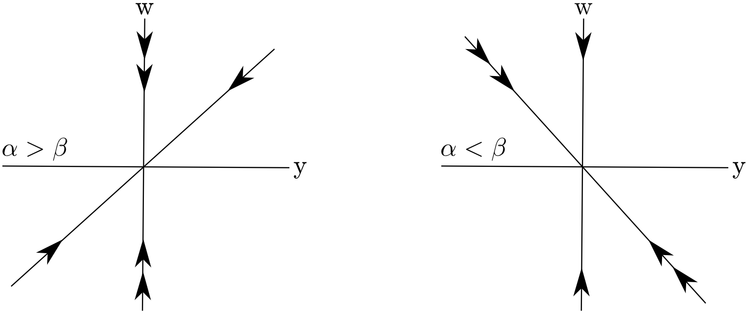
Figure 3: Sketch of the strongly and weakly stable directions at a given point for system (1) with $f=0$ for the cases $\alpha>\beta$ and $\alpha<\beta$.

The results of this article suggest that for uni-directionally coupled (skew-product) systems where the Kaplan-Yorke equality is robustly violated there should be still a meaningful relation between the information dimension of the physical measure and the Lyapunov exponents. However, the relation must distinguish between the Lyapunov exponents of the drive system (the “base”, in the language of skew-product systems) and those associated with the response system (the “fiber”). To be precise, let $\mu$ be a physical measure for the combined drive-response system. The projection of $\mu$ onto the drive state space is invariant for the drive system, and its Lyapunov exponents $\lambda_{1}\geq\cdots\geq\lambda_{k}$ are also Lyapunov exponents of the combined system. Let $\chi_{1}\geq\cdots\geq\chi_{\ell}$ be the remaining Lyapunov exponents of the combined system. We conjecture that there is a function of the two vectors $(\lambda_{1},\dots,\lambda_{k})$ and $(\chi_{1},\dots,\chi_{\ell})$ that typically coincides with $D_{1}(\mu)$, and in this sense extends the Kaplan-Yorke conjecture to uni-directionally coupled systems. Our results indicate that depending on the relative ordering of the $\lambda_{i}$’s and the $\chi_{j}$’s, this function may coincide with the Lyapunov dimension of the combined set of exponents, or may coincide with the sum of the Lyapunov dimensions of the two sets of exponents considered separately. There may be other possibilities as well in higher dimensions. More generally, one can also consider systems with more than two subsystems and incomplete (not all-to-all) coupling. Also in this context, a very interesting question would be whether certain dimensions could be a measure for the connectivity of a network of coupled systems.

It seems that prevalence could be a good notion to define what “typical” means in the Kaplan-Yorke conjecture. But in the general case of arbitrary maps on manifolds we have no natural linear structure on the function space and nonlinear notions of prevalence are still subject of ongoing investigations, see [HK10].

References

• [AY84] J.C. Alexander and J.A. Yorke. Fat baker’s transformations. Ergodic Theory and Dynamical Systems, 4(1):1–23, 1984.
• [Bar08] L. Barreira. Dimension and Recurrence in Hyperbolic Dynamics, volume 272 of Progress in Mathematics. Birkhaeuser, 2008.
• [Bau92] H. Bauer. Maß- und Integrationstheorie. Gruyter, 2nd edition, 1992.
• [BBD+88] R. Badii, G. Broggi, B. Derighetti, M. Ravani, S. Ciliberto, A. Politi, and M. A. Rubio. Dimension increase in filtered chaotic signals. Physical Review Letters, 60:979–982, 1988.
• [BGT01] J.-M. Barbaroux, F. Germinet, and S. Tcheremchantsev. Generalized fractal dimensions: equivalences and basic properties. Journal des Mathématiques Pures et Appliqués, 80(10):977–1012, 2001.
• [BHM92] D. S. Broomhead, J. P. Huke, and M. R. Muldoon. Linear filters and non-linear systems. Journal of the Royal Statistical Society. Series B (Methodological), 54(2):373–382, 1992.
• [BP86] R. Badii and A. Politi. On the Fractal Dimension of Filtered Chaotic Signals. In G. Mayer-Kress, editor, Dimensions and Entropies in Chaotic Systems, pages 67–73. Springer, 1986.
• [BP02] L. Barreira and Ya.B. Pesin. Lyapunov Exponents and Smooth Ergodic Theory, volume 23 of University Lecture Series. American Mathematical Society, 2002.
• [Bro76] J. R. Brown. Ergodic theory and topological dynamics, volume 70 of Pure and applied mathematics. Academic Press, 1976.
• [Che93] Z.-M. Chen. A note on Kaplan-Yorke-type estimates on the fractal dimension of chaotic attractors. Chaos, Solitons & Fractals, 3(5):575–582, 1993.
• [CI01] V.V. Chepyzhov and A.A. Ilyin. A note on the fractal dimension of attractors of dissipative dynamical systems. Nonlinear Analysis, 44(6):811–819, 2001.
• [Cut91] C.D. Cutler. Some results on the behavior and estimation of the fractal dimensions of distributions on attractors. Journal of Statistical Physics, 62(3-4):651–708, 1991.
• [DC96] M.E. Davies and K.M. Campbell. Linear recursive filters and nonlinear dynamics. Nonlinearity, 9(2):487–499, 1996.
• [Dug89] J. Dugundji. Topology. Brown, 1989.
• [Fal97] K. Falconer. Techniques in Fractal Geometry. John Wiley, 1997.
• [Fal03] K. Falconer. Fractal Geometry. 2nd. John Wiley, 2003.
• [FKYY83] P. Frederickson, J.L. Kaplan, E.D. Yorke, and J.A. Yorke. The liapunov dimension of strange attractors. Journal of Differential Equations, 49(2):185–207, 1983.
• [FOY83] J.D. Farmer, E. Ott, and J.A. Yorke. The dimension of chaotic attractors. Physica D Nonlinear Phenomena, 7(1-3):153–180, 1983.
• [HK97] B.R. Hunt and V.Yu. Kaloshin. How projections affect the dimension spectrum of fractal measures. Nonlinearity, 10(5):1031–1046, 1997.
• [HK10] B.R. Hunt and V.Yu. Kaloshin. Prevalence. In H. Broer, F. Takens, and B. Hasselblatt, editors, Handbook of Dynamical Systems, volume 3, pages 43–87. Elsevier Science, 2010.
• [HP83] H.G.E. Hentschel and I. Procaccia. The infinite number of generalized dimensions of fractals and strange attractors. Physica D: Nonlinear Phenomena, 8(3):435–444, 1983.
• [HSY92] B.R. Hunt, T. Sauer, and J.A. Yorke. Prevalence: a translation-invariant “almost every” on infinite-dimensional spaces. Bulletin of the American Mathematical Society, 27(2):217–238, 1992.
• [KMPY84] J.L. Kaplan, J. Mallet-Paret, and J.A. Yorke. The Lyapunov dimension of a nowhere differentiable attracting torus. Ergodic Theory and Dynamical Systems, 4(2):261–281, 1984.
• [KP08] S.G. Krantz and H.R. Parks. Geometric Integration Theory. Cornerstones. Birkhäuser, 2008.
• [KY79] J.L. Kaplan and J.A. Yorke. Chaotic behavior of multidimensional difference equations. In Functional Differential Equations and Approximation of Fixed Points, volume 730 of Lecture Notes in Mathematics, pages 204–227. Springer, 1979.
• [LY88] F. Ledrappier and L.-S. Young. Dimension formula for random transformations. Communications in Mathematical Physics, 117(4):529–548, 1988.
• [MML88] F. Mitschke, M. Möller, and W. Lange. Measuring filtered chaotic signals. Physical Review A, 37:4518–4521, 1988.
• [MR07] J. Myjak and R. Rudnicki. On the information dimensions. Bollettino dell unione matematica italiana. Sezione B, 10(2):357–364, 2007.
• [OY05] W. Ott and J.A. Yorke. Prevalence. Bulletin of the American Mathematical Society, 42(3):263–290, 2005.
• [PC96] L.M. Pecora and T.L. Carroll. Discontinuous and nondifferentiable functions and dimension increase induced by filtering chaotic data. Chaos: An Interdisciplinary Journal of Nonlinear Science, 6(3):432–439, 1996.
• [SD94] J. Stark and M. Davies. Recursive filters driven by chaotic signals. In Exploiting Chaos in Signal Processing, IEE Colloquium on, page 5/1–5/16, 1994.
• [Sta97] J. Stark. Invariant graphs for forced systems. Physica D: Nonlinear Phenomena, 109(1-2):163–179, 1997. Proceedings of the Workshop on Physics and Dynamics between Chaos, Order, and Noise.
• [Sta99] J. Stark. Regularity of invariant graphs for forced systems. Ergodic Theory and Dynamical Systems, 19(1):155–199, 1999.
• [SY97] T.D. Sauer and J.A. Yorke. Are the dimensions of a set and its image equal under typical smooth functions? Ergodic Theory and Dynamical Systems, 17(4):941–956, 1997.
• [Wal82] P. Walters. An Introduction To Ergodic Theory, volume 79 of Graduate Texts in Mathematics. Spinger, 1982.
• [You82] L.-S. Young. Dimension, entropy and Lyapunov exponents. Ergodic Theory and Dynamical Systems, 2(1):109–124, 1982.
• [You02] L.-S. Young. What Are SRB Measures, and Which Dynamical Systems Have Them? Journal of Statistical Physics, 108(5):733–754, 2002.