Relaxation and Rheology in Dense Athermal Suspensions

Abstract

We study relaxation and rheology of dense athermal suspensions of frictionless particles close below the jamming density. Our key quantity, the relaxation time—determined from the exponential decay of the energy after the shearing has suddenly been switched off—is argued to be a determining factor behind the algebraic divergence of various quantities as the jamming density is approached from below. We also define and measure the “dissipation time”, which is obtained directly in shearing simulations and find that it behaves similarly to the relaxation time. Comparing shear viscosity with the expression for the dissipation time we identify a non-divergent factor that explains the need for correction terms in the scaling analyses of the shear viscosity.

As the volume fraction increases in zero-temperature collections of spherical particles with repulsive contact interaction, there is a transition from a liquid to an amorphous solid state—the jamming transition. This transition has for quite some time been studied through simulations in two different ways: by examining static packings generated by compressing and relaxing random packings, and by driving the system with a shear deformation. Whereas it was first commonly expected that these two approaches would show the same behavior, the evidence now suggest that they are clearly different. One example is the difference in the behavior of the pressure above the jamming density, $\phi_{J}$, $p(\phi)\sim(\phi-\phi_{J})^{y}$, which is linear, $y=1$ for static packingsOHern_Langer_Liu_Nagel:2002 but appears to be $y\approx 1.1$ for the shear-driven caseOlsson_Teitel:gdot-scale . Another example is the isolated mode in the spectrum that dominates the behavior of the shear-driven system close to the transitionLerner-PNAS:2012 but which is not present in static packings.

One way to study the shear-driven transition is to try and eliminate the complications related to the softness of the particles and instead try and determine the behavior of hard particles. This is usually done by driving with sufficiently low shear rates, $\dot{\gamma}$, such that the particle overlaps become negligable—this is the linear region where many quantities are linear in $\dot{\gamma}$ (see e.g. Fig. 1 in LABEL:Olsson_Teitel:jam-HB). This is so since in the strict hard core limit one expects particles driven with different $\dot{\gamma}$, to follow the same path through phase space, only with different velocities $\mathbf{v}_{i}\propto\dot{\gamma}$, and it then follows that many quantities (e.g. the forces) are just proportional to $\dot{\gamma}$Olsson_Teitel:jam-HB ; Andreotti:2012 . The alternative is a recently deviced method to perform shearing simulations with hard particlesLerner-PNAS:2012 ; Lerner-Comp:2013 .

The transition in shear-driven systems still appears to be rather poorly understood. There is e.g. no accepted value for the exponent for the divergence of the viscosity; determined values range between 2.0 and 2.8Olsson_Teitel:jamming ; Hatano:2008 ; Otsuki_Hayakawa:2009b ; Bonnoit:2010 ; Olsson_Teitel:gdot-scale ; Boyer:2011 ; Andreotti:2012 , and this appears to, to at least some extent, be because of the lack of understanding of the mechanism behind this divergence. To illustrate the complications we point out that one typically expects both shear viscosity $\eta=\sigma/\dot{\gamma}$ and the pressure-equivalent quantity, $\eta_{p}=p/\dot{\gamma}$, to diverge in the same way, but since $\mu=\sigma/p=\eta/\eta_{p}$ has a pronounced density dependenceBoyer:2011 ; Lerner-PNAS:2012 in the relevant density interval, naive fits of $\eta(\phi)$ and $\eta_{p}(\phi)$ to algebraic divergences, $(\phi_{J}-\phi)^{-\beta}$, give differing values for the critical parameters. One way to resolve this issue is to include corrections to scaling in the analyses, but even though such a program has been successfully accomplishedOlsson_Teitel:gdot-scale , this requires very high precision data very close to the transition and the scaling analysis becomes both difficult and opaque.

In this Letter we present results from relaxation simulations which are done by first driving at a certain shear rate and then stopping the shearing and letting the system relax according to its dynamics. The relaxation time $\tau_{\mathrm{relax}}$ is then determined from the decay of the energy. We believe that this relaxation time is a fundamental quantity which is at the root of the divergence of pressure and shear viscosity. We also consider another time, $\tau_{\mathrm{diss}}$, which is related to the rate at which energy is dissipated in steady shearing and show that this quantity behaves similarly to $\tau_{\mathrm{relax}}$. We further show that $\eta$ and $\eta_{p}$ may be written as products of $\tau_{\mathrm{diss}}$ and some $\phi$-dependent correction factors, and we show that this picture nicely explains the need for corrections to scaling in the scaling analysis of LABEL:Olsson_Teitel:gdot-scale. The methods suggested here should be useful for studies of the jamming transition through both simulations and experiments.

We simulate frictionless soft disks in two dimensions using a bi-dispersive mixture with equal numbers of disks with two different radii of ratio 1.4. Length is measured in units of the diameter of the small particles ($d_{s}=1$). With $r_{ij}$ the distance between the centers of two particles, $d_{ij}$ the sum of their radii, and the relative overlap $\delta_{ij}=1-r_{ij}/d_{ij}$ for $r_{ij}<d_{ij}$ and $\delta_{ij}=0$ otherwise, the interaction between the particles is

$$V(r_{ij})=\epsilon\delta_{ij}^{2}/2,$$

with $\epsilon=1$. We use Lees-Edwards boundary conditions Evans_Morriss to introduce a time-dependent shear strain $\gamma(t)=t\dot{\gamma}$. With periodic boundary conditions on the coordinates $x_{i}$ and $y_{i}$ in an $L\times L$ system, the position of particle $i$ in a box with strain $\gamma$ is defined as $\mathbf{r}_{i}=(x_{i}+\gamma y_{i},y_{i})$. We simulate overdamped dynamics at zero temperature with the equation of motion Durian:1995 ,

$$\frac{d\mathbf{r}_{i}}{dt}=-\frac{1}{k_{d}}\sum_{j}\frac{dV(\mathbf{r}_{ij})}{d\mathbf{r}_{i}}+y_{i}\dot{\gamma}\;\hat{x},$$

with $k_{d}=1$. In this model dissipation occurs when the particles move relative to the steady shearing velocity $y_{i}\dot{\gamma}\hat{x}$. The effects of instead letting the dissipation be given by the relative velocity of particles in contact will be discussed elsewhereVagberg_Olsson_Teitel:NMF .

The key quantity in this Letter, the relaxation time, is determined through a two-step process: first the system is driven in steady shear at a constant shear rate $\dot{\gamma}$; then the shearing is stopped and the system is allowed to relax down to a minimum energy. As the simulations discussed here are at densities somewhat below $\phi_{J}$, the final state is always a state of zero energy, and after a short transient time, the decay is exponential,

$$E(t)\sim\exp(-t/\tau_{\mathrm{relax}}).$$

A few realisations of such relaxations are shown in Fig. 1. For each realisation the relaxation time is determined from the data with $E(t)<10^{-12}$, where the decay is exponential to an excellent approximation. We determine $\tau_{\mathrm{relax}}(\phi,\dot{\gamma})$ as the average relaxation time from about 10–100 such relaxations.

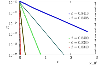
Figure 1: Relaxation of the energy at different $\phi$. The figure shows the relaxation of energy after the shearing has been switched off. The preceeding shearing simulations were performed at very low shear rates in order to stay close to the linear region; the densities and the initial shear rates were $(\phi,\dot{\gamma})=(0.834,10^{-8})$, $(0.838,10^{-8})$, $(0.840,5\times 10^{-9})$, $(0.8408,2\times 10^{-9})$, $(0.8416,10^{-9})$. To determine the relaxation times, $\tau_{\mathrm{relax}}$, we fit the energy to an exponential decay, only using data with $E<10^{-12}$.

Figure 2(a), which is $\tau_{\mathrm{relax}}$ versus $\phi$ in a narrow density interval just below $\phi_{J}$, shows that $\tau_{\mathrm{relax}}$ increases very rapidly with $\phi$. The data are shown for a few different $\dot{\gamma}$ and we conclude that $\tau_{\mathrm{relax}}$ at a given $\phi$ approaches a well-defined limiting value as $\dot{\gamma}$ decreases and the linear region is approached. In this Letter we analyze the data within (or close to) this linear region only; the behavior at larger $\dot{\gamma}$ will be examined elsewhere. We first determine the critical behavior from the eight points in Fig. 2(a) which are in the linear region and close below jamming, i.e. the points with the lowest shear rate for each density in the range $0.834\leq\phi\leq 0.8416$. Fitting these points to an algebraic divergence, $\tau_{\mathrm{relax}}(\phi)=A|\delta\phi|^{-\beta}$, (where $\delta\phi=\phi_{J}-\phi$) gives Fig. 2(b) and the critical parameters $\phi_{J}=0.8433\pm 0.0002$ and $\beta=2.73\pm 0.15$, which are in good agreement with Refs. Heussinger_Barrat:2009 ; Olsson_Teitel:gdot-scale . The quoted errors represent max/min-values, corresponding to three standard deviations in the estimated quantities.

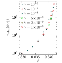
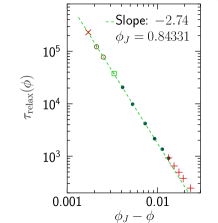
Figure 2: Behavior of the relaxation time. Panel (a) shows how $\tau_{\mathrm{relax}}$ depends on both $\phi$ and $\dot{\gamma}$, which is here the shear rate of the preparatory run (the relaxations are performed with $\dot{\gamma}=0$). Each value here is the average of relaxation times determined from of a large number of different relaxations. At sufficiently low $\dot{\gamma}$, $\tau_{\mathrm{relax}}$ approaches well-defined values that only depend on $\phi$. Panel (b) is a double-log plot, only including the points with small enough $\dot{\gamma}$ to be in the linear region. The figure shows a fit to the eight points with $\phi\geq 0.834$; the points with $\phi_{J}-\phi>0.01$ are not included in the fit.

Our assumption is that this increase of the relaxation time as jamming is approached is the fundamental phenomenon which is at the root of the divergence of other quantities as e.g. the shear viscosity, $\eta$. The relaxation mode should be related to the isolated mode with frequency $\omega_{\mathrm{min}}$ in LABEL:Lerner-PNAS:2012, and we expect $\tau_{\mathrm{relax}}\sim\omega_{\mathrm{min}}^{-2}$. (The different powers of time here reflect the differences in dynamics. In overdamped dynamics there is a velocity that is proporional to a force, whereas one in vibrational analyses assumes Newtonian dynamics with massive particles where the acceleration is proportional to the force.) Note also that the lowest mode being isolated explains why the relaxation is almost perfectly exponential after the initial decay. One would otherwise typically expect $E(t)$ to be given by a sum of several modes with close but different time constants. A further result from LABEL:Lerner-PNAS:2012,_Lerner-epl:2012 is that $\omega_{\mathrm{min}}^{-2}$ (and thereby $\tau_{\mathrm{relax}}$) diverges with the same exponent as the shear viscosity. This conclusion will also be reached below in a different way.

We will now try and establish a link between the shear viscosity, $\eta$, which is typically measured in both simulations and experiments, and the above obtained $\tau_{\mathrm{relax}}$. This will be done in two steps: we first derive an expression for a similar time, $\tau_{\mathrm{diss}}$, which is obtained directly in the shear driven simulations; we then express $\eta$ in terms of $\tau_{\mathrm{diss}}$.

The expression for the dissipation time, $\tau_{\mathrm{diss}}$, is obtained from a power balance. The idea is that the supplied power, which is $\sigma\dot{\gamma}$ per unit area, on average should be balanced by the dissipated power. Defining $\tau_{\mathrm{diss}}$ such that $E/\tau_{\mathrm{diss}}$ is the rate at which the energy is dissipated defines

$$\tau_{\mathrm{diss}}=\frac{E}{\sigma\dot{\gamma}}.$$ (1)

Note that it follows directly that $\tau_{\mathrm{diss}}$ should diverge with the exponent $\beta$ since $\sigma/\dot{\gamma}\sim|\delta\phi|^{-\beta}$ and $E/\dot{\gamma}^{2}\sim|\delta\phi|^{-2\beta}$Olsson_Teitel:jam-HB .

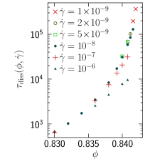
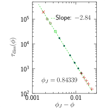
Figure 3: Dissipation time $\tau_{\mathrm{diss}}$ obtained in shear driven simulations. Panel (a) is $\tau_{\mathrm{diss}}$ against $\phi$ at different $\dot{\gamma}$. Panel (b) shows the data considered to be in the linear region against $\phi_{J}-\phi$. The dashed line shows the result of a fit to the eight points with $\phi_{J}-\phi<0.01$, giving $\phi_{J}=0.8434$ and $\beta=2.84$.

The dissipation time $\tau_{\mathrm{diss}}$ versus $\phi$ for a few different shear rates is shown in Fig. 3(a). Just as for $\tau_{\mathrm{relax}}$ we find that $\tau_{\mathrm{diss}}$ increases rapidly when $\phi$ increases towards $\phi_{J}$, and we also find well-defined low-$\dot{\gamma}$ limits, with deviations for larger $\dot{\gamma}$. Here $\tau_{\mathrm{diss}}$ becomes smaller for larger $\dot{\gamma}$, which is the same behavior as in the shear viscosity, but opposite to the behavior of $\tau_{\mathrm{relax}}$, discussed above.

The rational to introduce $\tau_{\mathrm{diss}}$ was to find a quantity in the shearing simulations that behaves similarly to $\tau_{\mathrm{relax}}$, and thus establish a link between the relaxation dynamics and the shearing simulations. It is however clear that these two quantities cannot be identical. Since the initial dissipation in a relaxation simulation has to be the same as the dissipation under steady shear, $\tau_{\mathrm{diss}}$ is equal to the initial decay rate in a relaxation simulation. $\tau_{\mathrm{relax}}$ on the other hand is the decay rate at long times. This means that $\tau_{\mathrm{diss}}$ should get contributions from all decay modes that are present in the system. $\tau_{\mathrm{relax}}$, on the other hand, is determined by the slowest mode only, since that is the only mode that persists after sufficiently long times. Since $\tau_{\mathrm{diss}}$ gets contributions from modes with smaller time constants it follows that $\tau_{\mathrm{diss}}<\tau_{\mathrm{relax}}$. This is confirmed by Fig. 4 which, furthermore, shows that $\tau_{\mathrm{diss}}/\tau_{\mathrm{relax}}$ increases with increasing $\phi$ and appears to approch unity as $\phi\to\phi_{J}$. We relate this to the observation in LABEL:Lerner-PNAS:2012 that the relative contribution to the shear viscosity of the isolated mode (in their notation, $\sigma_{0}/\sigma$) approaches unity as jamming is approached, which means that the weight of the other modes decreases. We likewise expect the contributions from the faster modes to $\tau_{\mathrm{diss}}$ to become less important as $\phi_{J}$ is approached, which implies $\tau_{\mathrm{diss}}/\tau_{\mathrm{relax}}\to 1$. We summarize the above in terms of two conclusions of importance for the present work: (i) Properties determined in steady shear will necessarily be different from the properties determined from the long-time behavior of the relaxation simulations. (ii) This difference is however rather small and one should therefore expect results based on $\tau_{\mathrm{relax}}$ and $\tau_{\mathrm{diss}}$, respectively, to be very similar.

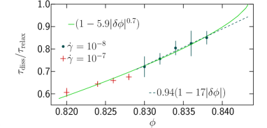
Figure 4: Relation between dissipation time and relaxation time. The figure shows that $\tau_{\mathrm{diss}}/\tau_{\mathrm{relax}}$ increases slowly as $\phi_{J}$ is approached from below. The solid line shows a fit to an algebraic function which approaches unity at $\phi_{J}$. The dashed line is a parametrization to help compare the size of this correction with the other corrections to scaling in Fig. 5.

A fit of $\tau_{\mathrm{diss}}$ to the algebraic divergence (where we again use only the eight points in the linear region and close to $\phi_{J}$) is shown in Fig. 3(b) and gives $\phi_{J}=0.8434\pm 0.0003$ and $\beta=2.84\pm 0.20$. Both values are close to (just slightly higher than) the corresponding values from the analysis of $\tau_{\mathrm{relax}}$, and this again suggests that $\tau_{\mathrm{diss}}$ is a good approximation of $\tau_{\mathrm{relax}}$.

The finding that $\tau_{\mathrm{diss}}$ to a good approximation diverges algebraically, gives a ground for understanding the need for corrections to scaling in the analyses of $\eta$ and $\eta_{p}$ in LABEL:Olsson_Teitel:gdot-scale. For the $\dot{\gamma}\to 0$ limit at densites below $\phi_{J}$, corrections to scaling means that the divergence cannot be well approximated by the algebraic $A|\delta\phi|^{-\beta}$ alone, but that one instead has to use

$$A|\delta\phi|^{-\beta}\left(1+a|\delta\phi|^{\omega\nu}\right),$$ (2)

which follows from using $b=|\delta\phi|^{-\nu}$ in the unnumbered equation before Eq. (3) in LABEL:Olsson_Teitel:gdot-scale. Here the correction to scaling exponent $\omega$ appears together with the correlation length exponent $\nu$. This behavior is illustrated in Fig. 5(a) which shows both $\eta$ and $\eta_{p}$ versus $\phi_{J}-\phi$. Also shown is $\eta_{E}=\sqrt{E}/\dot{\gamma}$ which behaves the same as $\eta_{p}$, to an excellent approximation. (This is so since $p\sim\sum_{ij}\delta_{ij}$ whereas $E\sim\sum_{ij}\delta^{2}_{ij}$Hatano:2009 .) As is clear from the figure, $\eta$ and $\eta_{p}$ behave differently, and attempts to determine $\beta$ from algebraic fits without corrections, give $\beta=2.35$ and $2.59$, respectively, as shown by the solid lines. Since one expects the asymptotic behavior of $\eta$ and $\eta_{p}$ to be the same, this discrepancy calls for including corrections to scaling (as in Eq. (2)), which was also done successfully in LABEL:Olsson_Teitel:gdot-scale.

We will now show that $\eta$ and $\eta_{E}$ may be written as products of $\tau_{\mathrm{diss}}$ and some correction factors. After introducing $\mu_{E}=\sigma/\sqrt{E}$ in analogy with the dimensionless friction $\mu=\sigma/p$ (see Fig. 5(b)) we find using Eq. (1) that

$$\eta = \sigma/\dot{\gamma}=\mu_{E}^{2}\;\tau_{\mathrm{diss}},$$ (3)

$$\eta_{E} = \sqrt{E}/\dot{\gamma}=\mu_{E}\;\tau_{\mathrm{diss}}.$$ (4)

We note two things: (i) That the corrections of $\eta$ and $\eta_{E}$ are $\mu_{E}^{2}$ and $\mu_{E}$, respectively gives a very direct explanation to why the correction to scaling in $\eta_{p}$ (which behaves essentially the same as $\eta_{E}$) is so much smaller than in $\eta$Olsson_Teitel:gdot-scale . See also below for a direct comparison of these correction terms. (ii) As shown in Fig. 5(b) $\mu^{2}_{E}$ (the correction factor that goes together with $\eta$) is linear in $\phi$ to an excellent approximation and the same holds for $\mu_{E}$, though in a more narrow range below $\phi_{J}$. Together with Eq. (2) we therefore conclude that $\omega\nu\approx 1$, again in agreement with LABEL:Olsson_Teitel:gdot-scale.

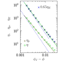
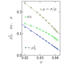
Figure 5: Viscosities $\eta$, $\eta_{p}$, and $\eta_{E}$ in the light of Eqs. (3) and (4). The dashed lines in panel (a) show the divergence of $\tau_{\mathrm{diss}}$ with $\beta=2.84$. The symbols show how $\eta$ and $\eta_{p}$ approach the presumed asymptotic scaling behavior, and it is clear that the corrections to scaling are much larger for $\eta$ than for $\eta_{p}$. The same is seen by naively fitting $\eta$ and $\eta_{p}$ to algebraic divergences (shown by solid lines) which give $\beta=2.35$ and $2.59$, respectively, where we note that the exponent obtained for $\eta$ is further off the asymptotic value $\beta=2.84$. Panel (b) shows both $\mu_{E}=\sigma/\sqrt{E}$, the similar dimensionless friction $\mu=\sigma/p$, and $\mu^{2}_{E}$ (the correction in Eq. (3)). This last quantity appears to be linear in $\phi$, which is consistent with $\omega\nu\approx 1$ as found in LABEL:Olsson_Teitel:gdot-scale.

As discussed above our starting assumption is that $\tau_{\mathrm{relax}}$ diverges algebraically and it then follows from Fig. 4 that $\tau_{\mathrm{diss}}$ is given by this algebraic divergence times a correction factor. To argue that the critical behavior should be determined from $\tau_{\mathrm{diss}}$ rather than $\eta$ or $\eta_{p}$, we now want to show that this correction in $\tau_{\mathrm{diss}}$ that one cannot eliminate (if one only has access to data from steady shearing) is considerably smaller than the correction factors in $\eta$ and $\eta_{E}$. To do that we write each correction on the form $(1+a|\delta\phi|)$ and compare the magnitude of “$a$” for the different cases. We then find $\mu_{E}^{2}\approx 0.0035(1+228|\delta\phi|)$ and (close to $\phi_{J}$) $\mu_{E}\approx 0.061(1+88|\delta\phi|)$ and note that both these correction terms are clearly bigger than the correction in $\tau_{\mathrm{diss}}/\tau_{\mathrm{relax}}\sim(1-17|\delta\phi|)$ from Fig. 4not-linear . This strengthens our confidence in the use of $\tau_{\mathrm{diss}}$ for determining the critical behavior, though it is of course $\tau_{\mathrm{relax}}$ that is the ideal quantity for such analyses.

The results above should also be useful for analyzing experiments, but instead of using $\tau_{\mathrm{diss}}=E/\sigma\dot{\gamma}$ one could then make use of $\tau_{\mathrm{diss}}\approx p^{2}/\sigma\dot{\gamma}$ which is an expression in terms of pressure instead of the elastic energy. This could be advantageous since pressure should be more readily available in experiments than energy.

The relaxation dynamics around the jamming transition has been studied before, but then with a rather different preparation of the starting configurations Hatano:2009 . In that study configurations were first generated randomly, then relaxed to a zero-energy state with the conjugate gradient method, and after that perturbed by a pure affine shear deformation. The relaxation time was then determined from the relaxation of such initial states by fitting the shear stress to $\sigma(\phi,t)\sim t^{-\alpha}e^{-t/\tau}$ with $\alpha=0.55(5)$, and was found to diverge as $\tau\sim(\phi_{J}-\phi)^{-\zeta}$ with $\zeta=3.3(1)$. This exponent is clearly bigger than our $\beta=2.73\pm 0.15$. One possible explanation for this difference is that in the present study we have been very careful to apply a slow shear driving in the preparation step, whereas they in their work apply the pure shear deformation suddenly, which should be more like a rapid shearing. Indeed, as shown in Fig. 2(b) any given fixed shear rate would give too large values for $\tau_{\mathrm{relax}}$ as one gets close to $\phi_{J}$, and from analyses of such data one would expect to get a too high value of the exponent for the divergence.

To conclude, we have determined $\tau_{\mathrm{relax}}$ from relaxational simulations and suggest that the slowing down of the relaxation as $\phi_{J}$ is approached is the fundamental reason for the divergence of $\eta$ and other similar quantities. Strong support for this idea is obtained from the finding by others that there is an isolated mode that dominates the behaviour close to $\phi_{J}$Lerner-PNAS:2012 . We have further introduced $\tau_{\mathrm{diss}}$ which is determined directly in shear driven simulations and have shown that these two quantities, in the linear region and close to $\phi_{J}$, are very similar. From the connection between $\tau_{\mathrm{diss}}$ and $\eta$ we further argue that the need for corrections to scaling in analyses of $\eta$ and related quanties is largely due to the $\phi$-dependence of $\mu_{E}=\sigma/\sqrt{E}$. Our results should also be helpful for getting more accurate determinations of the critical behaviour from experimental data.

I thank S. Teitel for helpful discussions and critical reading of the manuscript. This work was supported by the Swedish Research Council grant 2010-3725. Simulations were performed on resources provided by the Swedish National Infrastructure for Computing (SNIC) at PDC and HPC2N.

References

- (1) C. S. O’Hern, S. A. Langer, A. J. Liu, and S. R. Nagel, Phys. Rev. Lett. 88, 075507 (2002)
- (2) P. Olsson and S. Teitel, Phys. Rev. E 83, 030302(R) (2011)
- (3) E. Lerner, G. Düring, and M. Wyart, Proc. Nat. Acad. Sci. USA 109, 4798 (2012)
- (4) P. Olsson and S. Teitel, Phys. Rev. Lett. 109, 108001 (2012)
- (5) B. Andreotti, J.-L. Barrat, and C. Heussinger, Phys. Rev. Lett. 109, 105901 (2012)
- (6) E. Lerner, G. Düring, and M. Wyart, Computer Physics Communications 184, 628 (2013)
- (7) P. Olsson and S. Teitel, Phys. Rev. Lett. 99, 178001 (2007)
- (8) T. Hatano, J. Phys. Soc. Jpn. 77, 123002 (2008)
- (9) M. Otsuki and H. Hayakawa, Phys. Rev. E 80, 011308 (2009)
- (10) C. Bonnoit, T. Darnige, E. Clement, and A. Lindner, Journal of Rheology 54, 65 (2010)
- (11) F. Boyer, E. Guazzelli, and O. Pouliquen, Phys. Rev. Lett. 107, 188301 (2011)
- (12) D. J. Evans and G. P. Morriss, Statistical Mechanics of Nonequilibrium Liquids (Academic Press, London, 1990)
- (13) D. J. Durian, Phys. Rev. Lett. 75, 4780 (Dec 1995)
- (14) D. Vågberg, P. Olsson, and S. Teitel, unpublished
- (15) C. Heussinger and J.-L. Barrat, Phys. Rev. Lett. 102, 218303 (2009)
- (16) E. Lerner, G. Düring, and M. Wyart, Europhys. Lett. 99, 58003 (2012)
- (17) T. Hatano, Phys. Rev. E 79, 050301 (2009)
- (18) The linear relation here is an approximate parametrization to help compare the size of the different correction terms. As shown in Fig. 4 we expect the true behaviour to be given by a different exponent.