Nonequilibrium shot noise spectrum through a quantum dot in the Kondo regime:
A master equation approach under self-consistent Born approximation

Abstract

We construct a number($n$)-resolved master equation (ME) approach under self-consistent Born approximation (SCBA) for noise spectrum calculation. The formulation is essentially non-Markovian and incorporates properly the interlay of the multi-tunneling processes and many-body correlations. We apply this approach to the challenging nonequilibrium Kondo system and predict a profound nonequilibrium Kondo signature in the shot noise spectrum. The proposed $n$-SCBA-ME scheme goes completely beyond the scope of the Born-Markovian master equation approach, in the sense of being applicable to the shot noise of transport under small bias voltage, in non-Markovian regime, and with strong Coulomb correlations as favorably demonstrated in the nonequilibrium Kondo system.

Beyond the average current, shot noise (current fluctuations) can provide deep insight into the nature of transport mechanisms But00 . In the past decade, most efforts have been devoted to the zero- and low-frequency noise, including also the full counting statistics Lev96 . However, even more information is stored in the finite-frequency (FF) current noise Mar01 ; Vish03 ; Nay06 ; Gab08 ; Hei09 . For instance, the FF noise is sensitive to quantum statistics, where a crossover between different statistics can be revealed in the frequency domain. Also, in the quantum regime, which is defined by frequencies higher than the applied voltage or temperature, the FF noise is a powerful tool to probe the characteristic timescales of the system dynamics associated with intrinsic excitations and interactions.

Among the various techniques for shot noise calculation (including the counting statistics), the master equation approach, particularly its number($n$)-resolved version Gur96 ; Sch01 ; Jau05 ; Li05 , might be the most convenient one. However, this technique is built largely on the 2nd-order Born-Markovian master equation, which limits thus its application only in zero- or low-frequency noise, and under large bias voltage. In this work, we will first extend the master equation approach beyond these limits, making it highly non-Markovian and properly account for the interplay of multiple tunneling and many-body correlations. We then apply this new approach to the challenging nonequilibrium Kondo system to calculate the FF noise spectrum, where a profound Kondo resonance behavior will be revealed.

The nonequilibroum Kondo system, with the Anderson impurity realized by transport through a small quantum dot (QD), has been attracted intensive attention in the past two decades Gor98 ; Kou98 ; Gla04 ; Ng88 ; Her91 ; MW92 ; MW9193 ; Ra94 ; Mar06 ; Gor08 ; Yan12 . Compared to the equilibrium Kondo effect, the nonequilibrium is characterized by a finite chemical potential difference of the two leads. As a result, the peak of the density of states (spectral function) splits into two peaks pinned at each chemical potential. The two peak structure is difficult to probe directly, by the usual dc measurements. Nevertheless, the shot noise can be a promising quantity to reveal the nonequilibrium Kondo effect, although much less is known about it. We notice that results on low-frequency noise measurements have only appeared very recently De09 ; Hei08 , while so far there are not yet reports on the FF noise measurements. A couple of theoretical studies Ng97 ; Her98 ; Kon07 ; Moc11 , however, revealed diverse signatures (Kondo anomalies) in the FF noise spectra, such as an “upturn” Ng97 or a spectral “dip” Moc11 appeared at frequencies $\pm eV/\hbar$ ($V$ is the bias voltage), as well as the Kondo singularity (discontinuous slope) at frequencies $\pm 2eV/\hbar$ in Ref. Her98 , or at $\pm eV/2\hbar$ in Ref. Moc11 . Also, it was pointed out in Ref. Her98 that the minimum (dip) developed at $\pm eV/\hbar$ is not relevant to the Kondo effect, since in the noninteracting case the noise has similar discontinuous slope at $\pm eV/\hbar$ as well.

In general we describe a transport setup by $H=H_{S}(a_{\mu}^{\dagger},a_{\mu})+H_{\rm res}+H^{\prime}$. Here $H_{S}$ is the Hamiltonian of the central system embedded between two leads, with $a^{\dagger}_{\mu}$ ($a_{\mu}$) the creation (annihilation) operator of the state $|\mu\rangle$. More specifically, for a small and strongly interacting quantum dot, with only a single level involved in transport to realize an artificial Anderson impurity, we have

$$H_{S}=\sum_{\mu=\uparrow,\downarrow}\left(\epsilon_{\mu}a_{\mu}^{\dagger}a_{\mu}+\frac{U}{2}n_{\mu}n_{\bar{\mu}}\right).$$ (1)

In this model we use $\mu$ to label the spin-up (“$\uparrow$”) and spin-down (“$\downarrow$”) states, and $\bar{\mu}$ corresponds to the opposite spin orientation. $\epsilon_{\mu}$ is the spin-dependent (single) energy level, and $U$ the on-site Coulomb repulsive energy (with $n_{\mu}=a_{\mu}^{\dagger}a_{\mu}$ the occupation number operator). The other two Hamiltonians, $H_{\rm res}$ and $H^{\prime}$, describe the leads and their tunnel coupling to the central system. They are modeled by, respectively, $H_{\rm res}=\sum_{\alpha=L,R}\sum_{k}\epsilon_{\alpha k}b^{\dagger}_{\alpha k}b_{\alpha k}$ and $H^{\prime}=\sum_{\alpha=L,R}\sum_{\mu k}(t_{\alpha\mu k}a^{\dagger}_{\mu}b_{\alpha k}+\rm{H.c.})$ with $b^{\dagger}_{\alpha k}$ ($b_{\alpha k}$) the creation (annihilation) operator of electron in state $|k\rangle$ of the left ($L$) and right ($R$) leads.

For the study of shot noise, the nonequilibrium Green’s function based calculation scheme is not efficient. In contrast, an alternative one, say, the particle-number($n$)-resolved master equation ($n$-ME) plus the MacDonald’s formula Mac62 , provides a much more convenient method for that purpose. Also, the $n$-ME is extremely suitable for studying the full counting statistics (FCS). To our knowledge, the existing $n$-ME scheme is only precise to the Born approximation (BA), i.e., up to the 2nd-order expansion of the tunnel Hamiltonian Gur96 ; Sch01 ; Jau05 ; Li05 . Unfortunately, however, this type of master equation cannot describe the small bias transport, since in this case the multiple tunneling process between the system and lead is heavily involved. For similar reason, obviously, it cannot at all describe the Kondo effect, which is actually a consequence of interplay of the multiple tunneling and the many-body correlation. Therefore, in order to study the shot noise behavior through an interacting QD in the Kondo regime, one has to include the effect of higher order tunneling process in the master equation. In a recent work LJL11 , going beyond the Born approximation, an improved scheme under the self-consistent Born approximation was proposed as follows:

$$\dot{\rho}(t) =-i{\cal L}\rho(t)-\sum_{\mu\sigma}\Big{\{}\big{[}a^{\bar{\sigma}}_{\mu},{\cal A}^{(\sigma)}_{\mu\rho}(t)\big{]}+{\rm H.c.}\Big{\}}.$$ (2)

Here we set the Planck constant $\hbar=1$ and will make further convention in the following for a system of units by setting $e=k_{B}=1$ for the electron charge and the Boltzmann constant. In Eq. (2), we define: $\sigma=+$ and $-$, $\bar{\sigma}=-\sigma$; $a^{+}_{\mu}=a^{\dagger}_{\mu}$, and $a^{-}_{\mu}=a_{\mu}$. Also, the superoperators in Eq. (2) read ${\cal L}\rho=[H_{S},\rho]$ and ${\cal A}^{(\sigma)}_{\mu\rho}(t)=\sum_{\alpha=L,R}{\cal A}^{(\sigma)}_{\alpha\mu\rho}(t)$ while ${\cal A}^{(\sigma)}_{\alpha\mu\rho}(t)=\sum_{\nu}\int^{t}_{0}d\tau C^{(\sigma)}_{\alpha\mu\nu}(t-\tau)\left\{{\cal U}(t,\tau)[a^{\sigma}_{\nu}\rho(\tau)]\right\}$. $C^{(\sigma)}_{\alpha\mu\nu}(t-\tau)$ is the reservoir correlation function (see Appendix A for more details). Very importantly, ${\cal U}(t,\tau)$ is an effective propagator under the spirit of SCBA, which considerably generalizes the $H_{S}$-defined free propagator ${\cal G}(t,\tau)=e^{-i{\cal L}(t-\tau)}$ in the 2nd-order Born master equation. The SCBA is implemented by defining $\tilde{\rho}_{j}(t)\equiv{\cal U}(t,\tau)[a^{\sigma}_{\nu}\rho(\tau)]$ (here and in the following we use “$j$” to denote the double indices $(\nu,\sigma)$ for the sake of brevity), and closing Eq. (2) via an equation-of-motion (EOM) for this auxiliary object:

$$\dot{\tilde{\rho}}_{j}(t)=-i{\cal L}\tilde{\rho}_{j}(t)-\int^{t}_{\tau}dt^{\prime}\Sigma^{(A)}_{2}(t-t^{\prime})\tilde{\rho}_{j}(t^{\prime}).$$ (3)

In this equation the 2nd-order self-energy superoperator, $\Sigma^{(A)}_{2}(t-t^{\prime})$, differs from the usual one since it involves anticommutators, but not the commutators in the 2nd-order master equation (See Appendix A for an explicit expression).

Now we proceed further to construct the particle number (“$n$”) resolved SCBA-ME. To be specific, consider the reduced system state $\rho^{(n)}$, conditioned on the electron number arrived to the right lead, which satisfies

$$\dot{\rho}^{(n)} =-i{\cal L}\rho^{(n)}-\sum_{\mu}\Big{\{}\big{[}a_{\mu}^{\dagger}{\cal A}_{\mu\tilde{\rho}^{(n)}}^{(-)}+a_{\mu}{\cal A}_{\mu\tilde{\rho}^{(n)}}^{(+)}-{\cal A}_{L\mu\tilde{\rho}^{(n)}}^{(-)}a_{\mu}^{\dagger}$$

$$-{\cal A}_{L\mu\tilde{\rho}^{(n)}}^{(+)}a_{\mu}-{\cal A}_{R\mu\tilde{\rho}^{(n-1)}}^{(-)}a_{\mu}^{\dagger}-{\cal A}_{R\mu\tilde{\rho}^{(n+1)}}^{(+)}a_{\mu}\big{]}+{\rm H.c.}\Big{\}}.$$ (4)

Here ${\cal A}^{(\sigma)}_{\alpha\mu\tilde{\rho}^{(n)}}(t)=\sum_{\nu}\int^{t}_{0}d\tau C^{(\sigma)}_{\alpha\mu\nu}(t-\tau)[\tilde{\rho}_{j}^{(n)}(t,\tau)]$, while the summation over $\nu$ makes sense in regard to the abbreviation of $j=\{\nu,\sigma\}$. In particular, $\tilde{\rho}_{j}^{(n)}(t,\tau)$ is the $n$-dependent version of the quantity $\tilde{\rho}_{j}(t,\tau)={\cal U}(t,\tau)[a^{\sigma}_{\nu}\rho(\tau)]$, satisfying an EOM according to Eq. (3):

$$\dot{\tilde{\rho}}^{(n)}_{j} =-i{\cal L}\tilde{\rho}^{(n)}_{j}-\sum_{\mu}\Big{\{}\big{[}a_{\mu}^{\dagger}A_{\mu\tilde{\rho}^{(n)}_{j}}^{(-)}+a_{\mu}A_{\mu\tilde{\rho}^{(n)}_{j}}^{(+)}+A_{L\mu\tilde{\rho}^{(n)}_{j}}^{(-)}a_{\mu}^{\dagger}$$

$$+A_{L\mu\tilde{\rho}^{(n)}_{j}}^{(+)}a_{\mu}+A_{R\mu\tilde{\rho}^{(n-1)}_{j}}^{(-)}a_{\mu}^{\dagger}+A_{R\mu\tilde{\rho}^{(n+1)}_{j}}^{(+)}a_{\mu}\big{]}+{\rm H.c.}\Big{\}}.$$ (5)

In this equation we introduced $A^{(\sigma^{\prime})}_{\alpha\mu\tilde{\rho}^{(n)}_{j}}(t)=\sum_{\nu^{\prime}}\int^{t}_{\tau}dt^{\prime}C^{(\sigma^{\prime})}_{\alpha\mu\nu^{\prime}}(t-t^{\prime})\left\{e^{-i{\cal L}(t-t^{\prime})}[a^{\sigma^{\prime}}_{\nu^{\prime}}\tilde{\rho}_{j}^{(n)}(t^{\prime})]\right\}$.

The structure of Eq. (Nonequilibrium shot noise spectrum through a quantum dot in the Kondo regime: A master equation approach under self-consistent Born approximation) follows the same idea of constructing the 2nd-order $n$-resolved master equation Gur96 ; Li05 , which is essentially equivalent to the counting-field approach Sch01 ; Jau05 . Following Li05 , we split the Hilbert space of the electron reservoirs into a set of subspaces, each labeled by $n$. Then we do the average (trace) over each subspace and define the corresponding reduced quantities as $\rho^{(n)}(t)$ and $\tilde{\rho}^{(n)}_{j}(t,\tau)$. In Eq. (Nonequilibrium shot noise spectrum through a quantum dot in the Kondo regime: A master equation approach under self-consistent Born approximation), moreover, the appearance of $\tilde{\rho}^{(n\pm 1)}_{j}(t,\tau)$ is owing to a more tunneling event (forward/backword) involved in the process of the corresponding terms. These considerations also lead to the $n$-dependence structure of Eq. (Nonequilibrium shot noise spectrum through a quantum dot in the Kondo regime: A master equation approach under self-consistent Born approximation), the EOM of the auxiliary quantity $\tilde{\rho}^{(n)}_{j}$.

The noise spectrum, $S_{I}(\omega)$, is the Fourier transform of the current correlation function $S_{I}(t)=\langle I(t)I(0)\rangle_{ss}$ defined in the steady state. Very conveniently, within the framework of the $n$-ME, one can calculate $S_{I}(\omega)$ by using the MacDonald’s formula Mac62 : $S_{I}(\omega)=2\omega\int^{\infty}_{0}dt\sin(\omega t)\frac{d}{dt}\langle n^{2}(t)\rangle$, where $\langle n^{2}(t)\rangle=\sum_{n}n^{2}P(n,t)={\rm Tr}\sum_{n}n^{2}\rho^{(n)}(t)$, and the $n$-counting starts with the steady state ($\bar{\rho}$). Based on Eq. (Nonequilibrium shot noise spectrum through a quantum dot in the Kondo regime: A master equation approach under self-consistent Born approximation), one can express $\frac{d}{dt}\langle n^{2}(t)\rangle$ in terms of ${\cal A}^{(\sigma)}_{R\mu\bar{\rho}}(t)$ and ${\cal A}^{(\sigma)}_{R\mu\tilde{N}}(t)$. The former has been introduced in Eq. (2), needing only to replace $\rho(\tau)$ by $\bar{\rho}$. The latter reads ${\cal A}^{(\sigma)}_{R\mu\tilde{N}}(t)=\sum_{\nu}\int^{t}_{0}d\tau C^{(\sigma)}_{R\mu\nu}(t-\tau)[\tilde{N}_{j}(t,\tau)]$, where $\tilde{N}_{j}(t,\tau)=\sum_{n}n\tilde{\rho}_{j}^{(n)}(t,\tau)$. Then, the MacDonald’s formula becomes

$$S_{I}(\omega) =2\omega{\rm Im}\sum_{\mu}{\rm Tr}\Big{\{}2\big{[}{\cal A}_{R\mu\tilde{N}}^{(-)}(\omega)a_{\mu}^{\dagger}-{\cal A}_{R\mu\tilde{N}}^{(+)}(\omega)a_{\mu}\big{]}$$

$$\qquad\qquad+\big{[}{\cal A}_{R\mu\bar{\rho}}^{(-)}(\omega)a_{\mu}^{\dagger}+{\cal A}_{R\mu\bar{\rho}}^{(+)}(\omega)a_{\mu}\big{]}\Big{\}}.$$ (6)

This result is obtained after Laplace transforming ${\cal A}^{(\sigma)}_{R\mu\bar{\rho}}(t)$ and ${\cal A}^{(\sigma)}_{R\mu\tilde{N}}(t)$. More explicitly,

$${\cal A}^{(\sigma)}_{R\mu\bar{\rho}}(\omega)=\sum_{\nu}\int^{\infty}_{-\infty}\frac{d\omega^{\prime}}{2\pi}\Gamma^{(\sigma)}_{R\mu\nu}(\omega^{\prime}){\cal U}(\omega+\sigma\omega^{\prime})[a^{\sigma}_{\nu}\bar{\rho}(\omega)],$$

where the Laplace transformation of the steady state reads $\bar{\rho}(\omega)=i\bar{\rho}/\omega$, and the propagator ${\cal U}$ in frequency domain is defined through Eq. (3). On the other hand, ${\cal A}^{(\sigma)}_{R\mu\tilde{N}}(\omega)$ reads

$${\cal A}^{(\sigma)}_{R\mu\tilde{N}}(\omega)=\sum_{\nu}\int^{\infty}_{-\infty}\frac{d\omega^{\prime}}{2\pi}\Gamma^{(\sigma)}_{R\mu\nu}(\omega^{\prime})\tilde{\cal U}(\omega+\sigma\omega^{\prime})[a^{\sigma}_{\nu}N(\omega)].$$

In deriving this result, we introduced an additional propagator through $\tilde{N}_{j}(t,\tau)=\tilde{\cal U}(t-\tau)\tilde{N}_{j}(\tau)$, with $\tilde{N}_{j}(\tau)=a^{\sigma}_{\nu}N(\tau)$ as the initial condition which is defined by $N(\tau)=\sum_{n}n\rho^{(n)}(\tau)$. $\tilde{\cal U}(\omega)$ and $N(\omega)$ can be obtained via Laplace transforming the following EOMs. (i) For $N(\omega)$, based on the $n$-SCBA-ME we obtain

$$\dot{N}(t) =-i{\cal L}N(t)-\sum_{\mu\sigma}\Big{\{}\big{[}a^{\bar{\sigma}}_{\mu},{\cal A}^{(\sigma)}_{\mu N}(t)\big{]}+{\rm H.c.}\Big{\}}$$

$$~{}~{}+\sum_{\mu}\Big{\{}\big{[}{\cal A}_{R\mu\bar{\rho}}^{(-)}a_{\mu}^{\dagger}-{\cal A}_{R\mu\bar{\rho}}^{(+)}a_{\mu}\big{]}+{\rm H.c.}\Big{\}}.$$ (7)

(ii) For $\tilde{\cal U}(\omega)$, from Eq. (Nonequilibrium shot noise spectrum through a quantum dot in the Kondo regime: A master equation approach under self-consistent Born approximation) we have

$$\dot{\tilde{N}}_{j}(t)=-i{\cal L}\tilde{N}_{j}(t)-\int^{t}_{\tau}dt^{\prime}{\Sigma}^{(A)}_{2}(t-t^{\prime})\tilde{N}_{j}(t^{\prime})$$

$$~{}-\sum_{\mu}\Big{\{}\big{[}A_{R\mu\tilde{\rho}_{j}}^{(-)}(t)a_{\mu}^{\dagger}-A_{R\mu\tilde{\rho}_{j}}^{(+)}(t)a_{\mu}\big{]}+{\rm H.c.}\Big{\}}.$$ (8)

The self-energy superoperator ${\Sigma}^{(A)}_{2}(t-t^{\prime})$ is referred to Eq. (A.2) in Appendix A for its definition. Similar as introduced in Eq. (Nonequilibrium shot noise spectrum through a quantum dot in the Kondo regime: A master equation approach under self-consistent Born approximation), we defined here $A^{(\sigma^{\prime})}_{R\mu\tilde{\rho}_{j}}(t)=\sum_{\nu^{\prime}}\int^{t}_{\tau}dt^{\prime}C^{(\sigma^{\prime})}_{R\mu\nu^{\prime}}(t-t^{\prime})\left\{e^{-i{\cal L}(t-t^{\prime})}[a^{\sigma^{\prime}}_{\nu^{\prime}}\tilde{\rho}_{j}(t^{\prime})]\right\}$.

For the convenience of application, we would like to summarize the solving protocol in a more transparent way as follows. First, solve ${\cal U}(\omega)$ from Eq. (3) and obtain $\rho(\omega)$ from Eq. (2); then, extract $\tilde{\cal U}(\omega)$ from Eq. (Nonequilibrium shot noise spectrum through a quantum dot in the Kondo regime: A master equation approach under self-consistent Born approximation) and $N(\omega)$ from Eq. (Nonequilibrium shot noise spectrum through a quantum dot in the Kondo regime: A master equation approach under self-consistent Born approximation). With the help of ${\cal U}(\omega)$, $\tilde{\cal U}(\omega)$ and $N(\omega)$, one can straightforwardly calculate the noise spectrum of Eq. (Nonequilibrium shot noise spectrum through a quantum dot in the Kondo regime: A master equation approach under self-consistent Born approximation).

Now we return to the Anderson impurity model. Simply, there are four states involved in transport: $|0\rangle$, $|\uparrow\rangle$, $|\downarrow\rangle$ and $|d\rangle$, which correspond to the empty, spin-up, spin-down and double occupancy states, respectively. With respect to these states, the reservoir correlation function $C^{(\pm)}_{\alpha\mu\nu}$ is diagonal, i.e., $C^{(\pm)}_{\alpha\mu\nu}(t)=\delta_{\mu\nu}C^{(\pm)}_{\alpha\mu}(t)$ and $\Gamma^{(\pm)}_{\alpha\mu\nu}=\Gamma^{(\pm)}_{\alpha\mu}\delta_{\mu\nu}$. Moreover, using these basis states, we can reexpress the electron operator in terms of the projection operator form, $a^{\dagger}_{\mu}=|\mu\rangle\langle 0|+(-1)^{\mu}|d\rangle\langle\bar{\mu}|$, where the convention $(-1)^{\uparrow}=1$ and $(-1)^{\downarrow}=-1$ is assumed. Since the shot noise spectrum is defined on the steady-state current fluctuations, we need first a solution of the steady state ($\bar{\rho}$). In steady state, one can express the key operator in Eq. (2) as ${\cal A}^{(\pm)}_{\alpha\mu\bar{\rho}}=\int^{\infty}_{-\infty}\frac{d\omega}{2\pi}\,\Gamma^{(\pm)}_{\alpha\mu}(\omega){\cal U}(\pm\omega)[a^{\pm}_{\mu}\bar{\rho}]$. Straightforwardly, after some algebra, we obtain LJL11

$${\cal U}(\omega)[a^{\dagger}_{\mu}\bar{\rho}] =\left[\lambda^{+}_{\mu}(\omega)|\mu\rangle\langle 0|+\kappa^{+}_{\mu}(\omega)(-1)^{\mu}|d\rangle\langle\bar{\mu}|\right],$$

$${\cal U}(-\omega)[a_{\mu}\bar{\rho}] =\left[\lambda^{-}_{\mu}(\omega)|0\rangle\langle\mu|+\kappa^{-}_{\mu}(\omega)(-1)^{\mu}|\bar{\mu}\rangle\langle d|\right].$$ (9)

In terms of the matrix elements of $\bar{\rho}$, the specific expressions of $\lambda^{\pm}_{\mu}(\omega)$ and $\kappa^{\pm}_{\mu}(\omega)$ are given in Appendix B. Substituting ${\cal A}^{(\pm)}_{\alpha\mu\bar{\rho}}$, with the result of Eq. (Nonequilibrium shot noise spectrum through a quantum dot in the Kondo regime: A master equation approach under self-consistent Born approximation), into Eq. (2) one can first obtain the steady state. Then, following the solving protocol outlined above, the noise spectrum can be carried out.

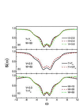
Figure 1: Shot noise spectrum in the Kondo regime, by varying the bias voltage (a), the temperature (b) and the bandwidth ($W$) of the reservoirs (c). We assume $\hbar=e=k_{B}=1$ and use an arbitrary unit of energy in this model simulation, with parameters as $\Gamma_{L}=\Gamma_{R}=\Gamma=0.5$, $\epsilon_{\uparrow}=\epsilon_{\downarrow}=\epsilon=-2$, and $U=6$. The bias voltage is defined as usual by $\mu_{L}=-\mu_{R}=V/2$. The Kondo temperature is given by $T_{K}=\frac{U}{2\pi}\sqrt{\frac{-2U\Gamma}{\epsilon(U+\epsilon)}}\exp[\frac{\pi\epsilon(U+\epsilon)}{2U\Gamma}]$, having a value of $T_{K}=0.144$ for the given parameters.

In Fig. 1 we display the symmetrized shot noise spectrum in Kondo regime (the numerical results are presented with the use of $\hbar=e=k_{B}=1$). First of all, we notice a remarkable dip behavior (Kondo signature) in the noise spectrum at the frequencies $\omega=\pm V/2$, as particularly demonstrated in Fig. 1(a) by altering the voltages. We attribute this behavior to the emergence of the Kondo resonance levels (KRLs) induced at the Fermi surfaces, i.e., at $\mu_{L}=V/2$ and $\mu_{R}=-V/2$. In steady state transport, it is well known that the KRLs are clearly reflected in the spectral function, i.e., the effective density of states (DOS) of the Anderson impurity. In terms of the master equation (see Appendix B), the KRLs structure is hidden in the self-energy terms, which characterize the tunneling process and define the transport current. Similarly, the noise spectrum is essentially affected, particularly in the Kondo regime, by the self-energy process in frequency domain based on the same master equation. This explains the emergence of the spectral dip appearing at the same KRLs (i.e., at $\omega=\pm V/2$).

However, we would like to remark that the dip behavior is also a consequence of highly non-Markovian treatment of the current correlations. We have checked that, using the quantum-jump technique Mil99 or the quantum regression theorem GZ00 , this behavior cannot be recovered, even the evolution during $(0,t)$ is treated as non-Markovian based on Eq. (2). The point is that the definition of the current in the correlation function $\langle I(t)I(0)\rangle$, in the non-Markovian case, cannot be independent of the propagation during the time interval $(0,t)$, because of the non-Markovian memory effect. In contrast, based on the $n$-SCBA-ME, the MacDonald formula correctly accounts for the correlation between the current and the memory effect during $(0,t)$, by employing the number($n$)-counting technique.

Alternatively, as a heuristic picture, one may imagine to include the KRLs as basis states in propagating $\rho(t)$, which is implied in the current correlation function. In usual case, when the level spacing is larger than its broadening, the diagonal elements of the density matrix decouple to the evolution of the off-diagonal elements. However, in the Kondo system, the diagonal and off-diagonal elements are coupled to each other, through the complicated self-energy processes. This feature would bring the coherence evolution described by the off-diagonal elements, with characteristic energies of the KRLs and their difference, into the diagonal elements which contribute directly to the the second current measurement in the correlation function $\langle I(t)I(0)\rangle$. Then, one may expect three coherence energies, $\pm V/2$ and $V$, to participate in the noise spectrum. Indeed, the dip emerged in Fig. 1 reveals the coherence-induced oscillation at the frequencies $\pm V/2$, while the other one at the higher frequency $V$ (observed in Ref. Moc11 in the case of infinite $U$) is smeared in our finite $U$ system by the rising noise with frequency.

Physically, the current fluctuation spectrum corresponds to electron transfer between the dot and leads, accompanied by the energy ($\omega$) absorption/emission of detection. Therefore, as the frequency ($\omega$) matches the energy difference between the dot level and the Fermi surface of the lead, certain “singularity” associated with the Fermi function at the Fermi surface is expected to emerge in the spectrum. This is reflected in Fig. 1(a) by the staircase behavior. This “singularity”, however, has been smoothed by the finite temperature effect (see Fig. 1(b) for further illustration). In Fig. 1(c) we display the bandwidth effect. For finite (narrow) bandwidth, the spectrum would diminish at high frequencies (when much higher than the bandwidth), since in this case the electron transfer channel associated with the $\omega$-emission/absorption is switched off. In the low frequency regime, on the other hand, we find that the narrowing bandwidth would shift the Kondo dip to lower frequency. This feature indicates that the Kondo peak pinned at the chemical potential is only a result in the wide band limit. For finite (especially narrow) bandwidths, it may need further work to determine the location of the Kondo peaks.

To summarize, we have applied a new shot noise scheme to the nonequilibrium Kondo system, for finite $U$ and arbitrary bandwidths. The scheme is based on a generalized number($n$)-resolved master equation under self-consistent Born approximation, which considerably goes beyond the scope of the usual 2nd-order Born master equation. This treatment allows us to predict a profound nonequilibrium Kondo signature in shot noise at frequencies associated with the chemical potentials. We anticipate a wide range of applications of the proposed approach to shot noise studies, as well as future work to clarify the diverse Kondo signatures in noise spectrum Ng97 ; Her98 ; Kon07 ; Moc11 .

Acknowledgements.— This work was supported by the NNSF of China, the Major State Basic Research Project of China under grants 2011CB808502 & 2012CB932704, and the Fundamental Research Funds for the Central Universities of China. J.J. was also supported by the Program for Excellent Young Teachers in Hangzhou Normal University and by the NSFC under No.11274085.

Appendix A Some Particulars in the SCBA-ME Approach

A.1 Reservoir Spectral Density Function

The key operators in Eq. (2) read ${\cal A}^{(\sigma)}_{\mu\rho}(t)=\sum_{\alpha=L,R}{\cal A}^{(\sigma)}_{\alpha\mu\rho}(t)$, and ${\cal A}^{(\sigma)}_{\alpha\mu\rho}(t)=\sum_{\nu}\int^{t}_{0}d\tau C^{(\sigma)}_{\alpha\mu\nu}(t-\tau)\left\{{\cal U}(t,\tau)[a^{\sigma}_{\nu}\rho(\tau)]\right\}$. $C^{(\sigma)}_{\alpha\mu\nu}(t-\tau)$ are the correlation functions of the reservoir electrons (in local equilibrium), being defined as

$$C^{(\sigma)}_{\alpha\mu\nu}(t-\tau)=\langle f^{(\sigma)}_{\alpha\mu}(t)f^{(\bar{\sigma})}_{\alpha\nu}(\tau)\rangle_{\rm B}.$$ (10)

Here, $f^{(+)}_{\alpha\mu}(t)=f^{\dagger}_{\alpha\mu}(t)$ and $f^{(-)}_{\alpha\mu}(t)=f_{\alpha\mu}(t)$, resulting from rewriting the tunneling Hamiltonian $H^{\prime}=\sum_{\alpha=L,R}\sum_{\mu k}(t_{\alpha\mu k}a^{\dagger}_{\mu}b_{\alpha\mu k}+\rm{H.c.})=\sum_{\alpha=L,R}\sum_{\mu}\left(a^{\dagger}_{\mu}f_{\alpha\mu}+\rm{H.c.}\right)$, by introducing $f_{\alpha\mu}=\sum_{k}t_{\alpha\mu k}b_{\alpha\mu k}$. The time dependence of the operators in $C^{(\sigma)}_{\alpha\mu\nu}(t-\tau)$ originates from using the interaction picture with respect to the reservoir Hamiltonian, while the average $\langle\cdots\rangle_{B}$ is over the reservoir states. Moreover, we introduce the Fourier transform of $C^{(\sigma)}_{\alpha\mu\nu}(t-\tau)$ through

$$C^{(\pm)}_{\alpha\mu\nu}(t-\tau)=\int^{\infty}_{-\infty}\frac{d\omega}{2\pi}e^{\pm i\omega(t-\tau)}\Gamma^{(\pm)}_{\alpha\mu\nu}(\omega).$$ (11)

Accordingly, we have $\Gamma^{(+)}_{\alpha\mu\nu}(\omega)=\Gamma_{\alpha\nu\mu}(\omega)n^{(+)}_{\alpha}(\omega)$ and $\Gamma^{(-)}_{\alpha\mu\nu}(\omega)=\Gamma_{\alpha\mu\nu}(\omega)n^{(-)}_{\alpha}(\omega)$, where $\Gamma_{\alpha\mu\nu}(\omega)=2\pi\sum_{k}t_{\alpha\mu k}t^{\ast}_{\alpha\nu k}\delta(\omega-\epsilon_{k})$ is the spectral density function of the reservoir ($\alpha$), $n^{(+)}_{\alpha}(\omega)$ denotes the Fermi function $n_{\alpha}(\omega)$, and $n^{(-)}_{\alpha}(\omega)=1-n_{\alpha}(\omega)$ is introduced for brevity. Alternatively, we may introduce as well the Laplace transform of $C^{(\sigma)}_{\alpha\mu\nu}(t-\tau)$, denoting by $C^{(\sigma)}_{\alpha\mu\nu}(\omega)$, which is related with $\Gamma^{(\pm)}_{\alpha\mu\nu}(\omega)$ through the well known dispersive relation:

$$C^{(\pm)}_{\alpha\mu\nu}(\omega) =\int^{\infty}_{-\infty}\frac{d\omega^{\prime}}{2\pi}\frac{i}{\omega\pm\omega^{\prime}+i0^{+}}\Gamma^{(\pm)}_{\alpha\mu\nu}(\omega^{\prime}).$$ (12)

In this work, for the reservoir spectral density function, we assume a Lorentzian form as

$$\Gamma_{\alpha\mu\nu}(\omega)=\frac{\Gamma_{\alpha\mu\nu}W^{2}_{\alpha}}{(\omega-\mu_{\alpha})^{2}+W^{2}_{\alpha}}.$$ (13)

In some sense, this assumption corresponds to a half-occupied band for each lead, which peaks the Lorentzian center at the chemical potential $\mu_{\alpha}$. $W_{\alpha}$ characterizes the bandwidth of the $\alpha$th lead. Obviously, the usual constant spectral density function is recovered from Eq. (13) in the limit $W_{\alpha}\rightarrow\infty$, yielding $\Gamma_{\alpha\mu\nu}(\omega)=\Gamma_{\alpha\mu\nu}$. Corresponding to the above Lorentzian spectral density function, straightforwardly, we obtain

$$C^{(\pm)}_{\alpha\mu\nu}(\omega) =\frac{1}{2}\left[\Gamma^{(\pm)}_{\alpha\mu\nu}(\mp\omega)+i\Lambda^{(\pm)}_{\alpha\mu\nu}(\mp\omega)\right].$$ (14)

The imaginary part, through the dispersive relation, is associated with the real one as

$$\Lambda^{(\pm)}_{\alpha\mu\nu}(\omega)={\cal P}\int^{\infty}_{-\infty}\frac{d\omega^{\prime}}{2\pi}\frac{1}{\omega\pm\omega^{\prime}}\Gamma^{(\pm)}_{\alpha\mu\nu}(\omega)$$

$$=\frac{\Gamma_{\alpha\mu\nu}}{\pi}\Bigg{\{}{\rm Re}\left[\Psi\left(\frac{1}{2}+i\frac{\beta(\omega-\mu_{\alpha})}{2\pi}\right)\right]$$

$$\quad-\Psi\left(\frac{1}{2}+\frac{\beta W_{\alpha}}{2\pi}\right)\mp\pi\frac{\omega-\mu_{\alpha}}{W_{\alpha}}\Bigg{\}},$$ (15)

where ${\cal P}$ stands for the principle value and $\Psi(x)$ is the digamma function.

A.2 Anomalous Self-Energy Superoperator

The central idea of the SCBA-ME scheme is replacing the free propagator in the 2nd-order master equation, ${\cal G}(t,\tau)=e^{-i{\cal L}(t-\tau)}$, by an effective one, ${\cal U}(t,\tau)$ under the SCBA spirit. By introducing $\tilde{\rho}_{j}(t)={\cal U}(t,\tau)[a^{\sigma}_{\nu}\rho(\tau)]$, we obtain Eq. (3), the EOM of this auxiliary object. In Eq. (3), the 2nd-order self-energy superoperator, $\Sigma^{(A)}_{2}(t-t^{\prime})$, is worth receiving some special attention. As labeled by the superscript “$(A)$”, an anticommutator, instead of the usual commutator, is involved there. That is, the self-energy superoperator has the following form:

$$\int^{t}_{\tau}dt^{\prime}\Sigma^{(A)}_{2}(t-t^{\prime}) \tilde{\rho}_{j}(t^{\prime})=\sum_{\mu}\Big{[}\big{\{}a_{\mu},A^{(+)}_{\mu\tilde{\rho}_{j}}\big{\}}+\big{\{}a^{\dagger}_{\mu},A^{(-)}_{\mu\tilde{\rho}_{j}}\big{\}}$$

$$+\big{\{}a^{\dagger}_{\mu},A^{(+)\dagger}_{\mu\tilde{\rho}_{j}}\big{\}}+\big{\{}a_{\mu},A^{(-)\dagger}_{\mu\tilde{\rho}_{j}}\big{\}}\Big{]},$$ (16)

where $A^{(\pm)}_{\mu\tilde{\rho}_{j}}$ is defined as $A^{(\sigma^{\prime})}_{\mu\tilde{\rho}_{j}}=\sum_{\alpha=L,R}\sum_{\nu^{\prime}}\int^{t}_{\tau}dt^{\prime}C^{(\sigma^{\prime})}_{\alpha\mu\nu^{\prime}}(t-t^{\prime})\left\{e^{-i{\cal L}(t-t^{\prime})}[a^{\sigma^{\prime}}_{\nu^{\prime}}\tilde{\rho}_{j}(t^{\prime})]\right\}$. We remark that the anticommutative brackets appeared in Eq. (A.2) indicate that the propagation of $\tilde{\rho}_{j}(t)$ does not satisfy the usual 2nd-order master equation. This actually violates the so-called quantum regression theorem.

A.3 Steady-State Current

Similar to the usual 2nd-order master equation approach, the current through the $\alpha$th lead reads

$$I_{\alpha}(t)=\frac{2e}{\hbar}\sum_{\mu}{\rm Re}\left\{{\rm Tr}\big{[}{\cal A}^{(+)}_{\alpha\mu\rho}(t)a_{\mu}-{\cal A}^{(-)}_{\alpha\mu\rho}(t)a^{\dagger}_{\mu}\big{]}\right\}.$$ (17)

Moreover, the steady state together with its associated current can be obtained easily as follows. Consider the integral $\int^{t}_{0}d\tau[\cdots]\rho(\tau)$ in ${\cal A}^{(\pm)}_{\alpha\mu\rho}(t)$. Since physically, the correlation function $C^{(\pm)}_{\alpha\mu\nu}(t-\tau)$ in the integrand is nonzero only on finite timescale, we can replace $\rho(\tau)$ in the integrand by the steady state $\bar{\rho}$, in the long time limit ($t\rightarrow\infty$). After this replacement, we obtain

$${\cal A}^{(\pm)}_{\alpha\mu\bar{\rho}}=\sum_{\nu}\int^{\infty}_{-\infty}\frac{d\omega}{2\pi}\,\Gamma^{(\pm)}_{\alpha\mu\nu}(\omega){\cal U}(\pm\omega)[a^{\pm}_{\nu}\bar{\rho}].$$ (18)

Then, substituting this result into Eq. (2), we can straightforwardly solve for $\bar{\rho}$ and calculate the steady state current.

We would like to mention that, remarkably, for noninteracting system, the steady state current given by this SCBA-ME scheme coincides precisely with the nonequilibrium Green’s function approach, both giving the exact result LJL11 . Notice also that, by contrast, the Born master equation is applicable only to sequential tunneling transport, being valid only in large bias limit.

Appendix B Steady State Solution of the Anderson Impurity Model

In Eq. (Nonequilibrium shot noise spectrum through a quantum dot in the Kondo regime: A master equation approach under self-consistent Born approximation), associated with the steady state solution of the Anderson impurity model, we have

$$\lambda^{+}_{\mu}(\omega) =i\frac{\Pi^{-1}_{1\mu}(\omega)\bar{\rho}_{00}-\Sigma^{-}_{\bar{\mu}}(\omega)\bar{\rho}_{\bar{\mu}\bar{\mu}}}{\Pi^{-1}_{\mu}(\omega)\Pi^{-1}_{1\mu}(\omega)},$$

$$\lambda^{-}_{\mu}(\omega) =i\frac{\Pi^{-1}_{1\mu}(\omega)\bar{\rho}_{\mu\mu}-\Sigma^{-}_{\bar{\mu}}(\omega)\bar{\rho}_{dd}}{\Pi^{-1}_{\mu}(\omega)\Pi^{-1}_{1\mu}(\omega)},$$

$$\kappa^{+}_{\mu}(\omega) =i\frac{-\Sigma^{+}_{\bar{\mu}}(\omega)\bar{\rho}_{00}+\Pi^{-1}_{\mu}(\omega)\bar{\rho}_{\bar{\mu}\bar{\mu}}}{\Pi^{-1}_{\mu}(\omega)\Pi^{-1}_{1\mu}(\omega)},$$

$$\kappa^{-}_{\mu}(\omega) =i\frac{-\Sigma^{+}_{\bar{\mu}}(\omega)\bar{\rho}_{\mu\mu}+\Pi^{-1}_{\mu}(\omega)\bar{\rho}_{dd}}{\Pi^{-1}_{\mu}(\omega)\Pi^{-1}_{1\mu}(\omega)}.$$ (19)

Here we introduced $\Pi^{-1}_{\mu}(\omega)=\omega-\epsilon_{\mu}-\Sigma_{0\mu}(\omega)-\Sigma^{+}_{\bar{\mu}}(\omega)$, and $\Pi^{-1}_{1\mu}(\omega)=\omega-\epsilon_{\mu}-U-\Sigma_{0\mu}(\omega)-\Sigma^{-}_{\bar{\mu}}(\omega)$. The self-energy $\Sigma_{0\mu}(\omega)$ is given by

$$\Sigma_{0\mu}(\omega) =\int^{\infty}_{-\infty}\frac{d\omega^{\prime}}{2\pi}\frac{\Gamma_{\mu}(\omega^{\prime})}{\omega-\omega^{\prime}+i0^{+}},$$ (20)

while $\Sigma^{\pm}_{\mu}(\omega)$ by

$$\Sigma^{\pm}_{\mu}(\omega) =\int\frac{d\omega^{\prime}}{2\pi}\frac{\Gamma^{(\pm)}_{\mu}(\omega^{\prime})}{\omega-\epsilon_{\bar{\mu}}+\epsilon_{\mu}-\omega^{\prime}+i0^{+}}$$

$$+\int\frac{d\omega^{\prime}}{2\pi}\frac{\Gamma^{(\pm)}_{\mu}(\omega^{\prime})}{\omega-E_{d}+\omega^{\prime}+i0^{+}}.$$ (21)

With the above results, as outlined after Eq. (Nonequilibrium shot noise spectrum through a quantum dot in the Kondo regime: A master equation approach under self-consistent Born approximation), one is able to carry out the steady state solution $\bar{\rho}$. Based on it, to obtain further the current, we first introduce $\varphi_{1\mu\nu}(\omega)={\rm Tr}\big{[}a_{\mu}\tilde{\rho}_{1\nu}(\omega)\big{]}$ and $\varphi_{2\mu\nu}(\omega)={\rm Tr}\big{[}a_{\mu}\tilde{\rho}_{2\nu}(\omega)\big{]}$, where $\tilde{\rho}_{1\nu}(\omega)$ and $\tilde{\rho}_{2\nu}(\omega)$ are calculated using Eq. (3), with an initial condition of $\tilde{\rho}_{1\nu}(0)=\bar{\rho}a^{\dagger}_{\nu}$ and $\tilde{\rho}_{2\nu}(0)=a^{\dagger}_{\nu}\bar{\rho}$. To simplify notations, we denote the various matrices in boldface form: $\bm{\varphi}_{1}(\omega)$, $\bm{\varphi}_{2}(\omega)$ and $\bm{\Gamma}_{L(R)}$. Now, if $\bm{\Gamma}_{L}$ is proportional to $\bm{\Gamma}_{R}$ by a constant, the steady state current can be recast to the Landauer-Büttiker type, in terms of an integration of tunneling coefficient over the incident energies, $\bar{I}=\frac{2e}{\hbar}{\rm Re}\int^{\infty}_{-\infty}\frac{d\omega}{2\pi}\left[n_{L}(\omega)-n_{R}(\omega)\right]{\cal T}(\omega)$. The tunneling coefficient, very compactly, is given by ${\cal T}(\omega)={\rm Tr}\{\bm{\Gamma}_{L}\bm{\Gamma}_{R}(\bm{\Gamma}_{L}+\bm{\Gamma}_{R})^{-1}{\rm Re}\big{[}\bm{\varphi}(\omega)\big{]}\}$, where $\bm{\varphi}(\omega)=\bm{\varphi}_{1}(\omega)+\bm{\varphi}_{2}(\omega)$. For the Anderson impurity system in nonequilibrium, we find

$$\bm{\varphi}(\omega)=\frac{i\big{[}\Pi^{-1}_{1\mu}(\omega)-\Sigma^{(+)}_{\bar{\mu}}(\omega)\big{]}(1-n_{\bar{\mu}})}{\Pi^{-1}_{\mu}(\omega)\Pi^{-1}_{1\mu}(\omega)-\Sigma^{(+)}_{\bar{\mu}}(\omega)\Sigma^{(-)}_{\bar{\mu}}(\omega)}$$

$$~{}~{}~{}~{}~{}~{}~{}~{}+\frac{i\big{[}\Pi^{-1}_{\mu}(\omega)-\Sigma^{(-)}_{\bar{\mu}}(\omega)\big{]}n_{\bar{\mu}}}{\Pi^{-1}_{\mu}(\omega)\Pi^{-1}_{1\mu}(\omega)-\Sigma^{(+)}_{\bar{\mu}}(\omega)\Sigma^{(-)}_{\bar{\mu}}(\omega)}$$

$$=\frac{i(1-n_{\bar{\mu}})}{\omega-\epsilon_{\mu}-\Sigma_{0\mu}+U\Sigma^{+}_{\bar{\mu}}(\omega-\epsilon_{\mu}-U-\Sigma_{0\mu}-\Sigma_{\bar{\mu}})^{-1}}$$

$$~{}~{}+\frac{in_{\bar{\mu}}}{\omega-\epsilon_{\mu}-U-\Sigma_{0\mu}-U\Sigma^{-}_{\bar{\mu}}(\omega-\epsilon_{\mu}-\Sigma_{0\mu}-\Sigma_{\bar{\mu}})^{-1}},$$ (22)

where $n_{\mu}=\rho_{\mu\mu}+\rho_{dd}$, and $1-n_{\mu}=\rho_{\bar{\mu}\bar{\mu}}+\rho_{00}$. This result, precisely, coincides with that given by the EOM technique of the nonequilibrium Green’s function Hau96 . One can check that, as discussed in detail in Ref. Hau96 , this solution contains the nonequilibrium Kondo effect.

References

• (1) Ya. M. Blanter and M. Büttiker, Phys. Rep. 336, 1 (2000); Quantum Noise in Mesoscopic Physics, edited by Yu. V. Nazarov (Kluwer, Dordrecht, 2003).
• (2) L. S. Levitov, H. W. Lee, and G. B. Lesovik, J. Math. Phys. 37, 4845 (1996).
• (3) I. Safi, P. Devillard, and T. Martin, Phys. Rev. Lett. 86, 4628 (2001).
• (4) S. Vishveshwara, Phys. Rev. Lett. 91, 196803 (2003).
• (5) C. Bena and C. Nayak, Phys. Rev. B 73, 155335 (2006).
• (6) J. Gabelli and B. Reulet, Phys. Rev. Lett. 100, 026601 (2008).
• (7) A. Bid, N. Ofek, M. Heiblum, V. Umansky, and D. Mahalu, Phys. Rev. Lett. 103, 236802 (2009).
• (8) S. A. Gurvitz and Ya. S. Prager, Phys. Rev. B 53, 15932 (1996).
• (9) Yu. Makhlin, G. Schön, and A. Shnirman, Rev. Mod. Phys. 73, 357 (2001).
• (10) C. Flindt, T. Novotny, and A. P. Jauho, Europhys. Lett. 69, 475 (2005).
• (11) X.-Q. Li, P. Cui, and Y. J. Yan, Phys. Rev. Lett. 94, 066803 (2005); X.-Q. Li, J. Luo, Y.-G. Yang, P. Cui, and Y. J. Yan, Phys. Rev. B 71, 205304 (2005).
• (12) D. Goldhaber-Gordon, H. Shtrikman, D. Mahalu, D. Abusch-Magder, U. Meirav, and M. A. Kastner, Nature 391, 156 (1998).
• (13) S. M. Cronenwett, T. H. Oosterkamp, and L. P. Kouwenhoven, Science 24, 540 (1998).
• (14) L. I. Glazman and M. Pustilnik, in Lectures notes of the Les Houches Summer School 2004 in “Nanophysics: Coherence and Transport”, edited by H. Bouchiat et al. (Elsevier, 2005), pp. 427-478.
• (15) T. K. Ng and P. A. Lee, Phys. Rev. Lett. 61, 1768 (1988).
• (16) S. Hershfield, J. H. Davies, and J. W. Wilkins, Phys. Rev. Lett. 67, 3720 (1991).
• (17) Y. Meir and N. S. Wingreen, Phys. Rev. Lett. 68, 2512 (1992).
• (18) Y. Meir, N. S. Wingreen, and P. A. Lee, Phys. Rev. Lett. 66, 3048 (1991); ibid. 70, 2601 (1993).
• (19) D. C. Ralph and R. A. Buhrman, Phys. Rev. Lett. 72, 3401 (1994).
• (20) J. Paaske, A. Rosch, P. Wölfle, N. Mason, C. M. Marcus, and J. Nygard, Nature Phys. 2, 460 (2006).
• (21) M. Grobis, I. G. Rau, R. M. Potok, H. Shtrikman, and D.Goldhaber-Gordon, Phys. Rev. Lett. 100, 246601 (2008).
• (22) Z. H. Li, N. H. Tong, X. Zheng, D. Hou, J. H. Wei, J. Hu, and Y. J. Yan, Phys. Rev. Lett. 109, 266403 (2012).
• (23) T. Delattre et al, Nature Phys. 5, 208 (2009).
• (24) O. Zarchin, M. Zaffalon, M. Heiblum, D. Mahalu, and V. Umansky, Phys. Rev. B 77, 241303 (2008).
• (25) G. H. Ding and T. K. Ng, Phys. Rev. B 56, 15521(R) (1997).
• (26) A. Schiller and S. Hershfield, Phys. Rev. B 58, 14978 (1998).
• (27) T. Korb, F. Reininghaus, H. Schoeller, and J. König, Phys. Rev. B 76, 165316 (2007).
• (28) C. P. Moca, P. Simon, C. H. Chung, and G. Zarand, Phys. Rev. B 83, 201303(R) (2011).
• (29) D. K. C. MacDonald, Noise and Fluctuations: an Introduction (Wiley, New York, 1962), Ch. 2.2.1.
• (30) J. Li, J. S. Jin, X. Q. Li, and Y. J. Yan, arXiv: 1110.4457
• (31) H. Haug and A.-P. Jauho, Quantum Kinetics in Transport and Optics of Semiconductors (2nd Ed., Springer-Verlag Berlin, 2007).
• (32) H. B. Sun and G. J. Milburn, Phys. Rev. B 59, 10748 (1999).
• (33) C. W. Gardiner and P. Zoller, Quantum Noise, 2nd ed. (Springer, New York, 2000).