Shape recognition and classification in electro-sensing

Abstract

This paper aims at advancing the field of electro-sensing. It exhibits the physical mechanism underlying shape perception for weakly electric fish. These fish orient themselves at night in complete darkness by employing their active electrolocation system. They generate a stable, high-frequency, weak electric field and perceive the transdermal potential modulations caused by a nearby target with different admittivity than the surrounding water. In this paper, we explain how weakly electric fish might identify and classify a target, knowing by advance that the latter belongs to a certain collection of shapes. The fish is able to learn how to identify certain targets and discriminate them from all other targets. Our model of the weakly electric fish relies on differential imaging, i.e., by forming an image from the perturbations of the field due to targets, and physics-based classification. The electric fish would first locate the target using a specific location search algorithm. Then it could extract, from the perturbations of the electric field, generalized (or high-order) polarization tensors of the target. Computing, from the extracted features, invariants under rigid motions and scaling yields shape descriptors. The weakly electric fish might classify a target by comparing its invariants with those of a set of learned shapes. On the other hand, when measurements are taken at multiple frequencies, the fish might exploit the shifts and use the spectral content of the generalized polarization tensors to dramatically improve the stability with respect to measurement noise of the classification procedure in electro-sensing. Surprisingly, it turns out that the first-order polarization tensor at multiple frequencies could be enough for the purpose of classification. A procedure to eliminate the background field in the case where the permittivity of the surrounding medium can be neglected, and hence improve further the stability of the classification process, is also discussed.

1 Introduction

In the turbid rivers of Africa and South America, some species of fish generate a stable, high frequency, weak electric field (0.1-10 kHz, $\leq 100$ mV/cm) which is not enough for defense purpose. In 1958, Lissmann and Machin [22] discovered that the emitted electrical signal is in fact used for active electro-sensing. The weakly electric fish have thousands of receptor organs at the surface of their skin. A nearby target with different admittivity than the surrounding water is detected by measurements of the electric organ discharge modulations at the receptor organs [13, 25]. Targets with large permittivity cause appreciable phase shifts, which can be measured by receptors called T-type units [26]. It is an important input for the fish, and thus it will be the central point in this paper for shape classification.

Active electro-sensing has driven an increasing number of experimental, behavioral, biological, and computational studies since Lissmann and Machin’s work [11, 12, 15, 17, 23, 24, 30, 36]. Behavioral experiments have shown that weakly electric fish are able to locate a target [36] and discriminate between targets with different shapes [35] or/and electric parameters (conductivity and permittivity) [33]. The growing interest in electro-sensing could be explained not only by the curiosity of discovering a “sixth sense”, the electric perception, that is not accessible by our own senses, but also by potential bio-inspired applications in underwater robotics. It is challenging to equip robots with electric perception and provide them, by mimicking weakly electric fish, with imaging and classification capabilities in dark or turbid environments [18, 19, 21, 27, 28, 32, 33].

Mathematically speaking, the problem is to locate the target and identify its shape and material parameters given the current distribution over the skin. Due to the fundamental ill-posedness character of this imaging problem, it is very intriguing to see how much information weakly electric fish are able to recover. The electric field due to the target is a complicated highly nonlinear function of its shape, admittivity, and distance from the fish. Thus, understanding analytically this electric sense is likely to give us insights in this regard [11, 12, 14, 15, 23, 27, 35]. While locating targets from the electric field perturbations induced on the skin of the fish is now understood (see [1, 21] and references therein), identifying and classifying their shapes is considered to be one of the most challenging problems in electro-sensing. Although the neuroethology of these fish has significantly been advanced last years (see [16] and references therein), the neural mechanisms encoding the shape of a target is far beyond the scope of our study. Rather, this work focuses on the physical feasibility of such a process, which was not explained until now.

In [1], a rigorous model for the electro-location of a target around the fish was derived. Using the fact that the electric current produced by the electric organ is time-harmonic with a known fundamental frequency, a space-frequency location search algorithm was introduced. Its robustness with respect to measurement noise and its sensitivity with respect to the number of frequencies, the number of sensors, and the distance to the target were illustrated. In the case of disk- and ellipse-shaped targets, the conductivity, the permittivity, and the size of the targets can be reconstructed separately from multifrequency measurements. Such measurements have been used successfully in trans-admittance scanners of breast tumors [10, 20, 31].

In this paper, we tackle the challenging problem of shape recognition and classification. In order to explain how the shape information is encoded in measured data, we first derive a multipolar expansion for the perturbations of the electric field induced by a nearby target in terms of the characteristic size of the target. Our asymptotic expansion generalizes Rasnow’s formula [29] in two directions: (i) it is a higher-order approximation of the effect of a nearby target and it is valid for an arbitrary shape and admittivity contrast and (ii) it takes also into account the fish’s body. As it has been first proved in [1], by postprocessing the measured data using layer potentials associated only to the fish’s body, one can reduce the multipolar formula to the one in free space, i.e., without the fish. Then we show how to identify and classify a target, knowing by advance that the latter belongs to a dictionary of pre-computed shapes. The shapes considered in this paper have been experimentally tested and results reported in [34]. This idea comes naturally in mind when modeling behavioral experiments such as in [33, 35, 36]. The pre-computed shapes would then be a model for the fish’s memory (trained to recognize specific shapes), and the experience of recognition presented here would simulate the discrimination exercises that are then imposed to them. We develop two algorithms for shape classification: one based on shape descriptors while the second is based on spectral induced polarizations. We first extract, from the data, generalized (or high-order) polarization tensors of the target (GPTs) [2]. These tensors, first introduced in [6], are intrinsic geometric quantities and constitute the right class of features to represent the target shapes [5, 9]. The shape features are encoded in the high-order polarization tensors. The extraction of the GPTs can be achieved by a least-squares method. The noise level in the reconstructed generalized polarization tensors depends on the angle of view. Larger is the angle of view, more stable is the reconstruction. $l_{1}$-regularization techniques could be used. Then we compute from the extracted features invariants under rigid motions and scaling. Comparing these invariants with those in a dictionary of pre-computed shapes, we successfully classify the target. Since the measurements are taken at multiple frequencies, we make use of the spectral content of the generalized polarization tensor in order to dramatically improve the stability with respect to measurement noise of the physics-based classification procedure. In fact, we show numerically that the first-order polarization tensor at multiple frequencies is enough for the purpose of classification.

2 Feature extraction from induced current measurements

2.1 Electro-sensing model

Let us recall the nondimensionalized model of electro-sensing: the body of the fish is $\Omega$ (of size of order $1$), an open bounded set in $\mathbb{R}^{d},d=2,3$, of class $\mathcal{C}^{1,\alpha}$, $0<\alpha<1$, with outward normal unit vector $\nu$. The electric organ is a dipole $f$ placed at $z_{0}\in\Omega$ or a sum of point sources inside $\Omega$ satisfying the neutrality condition. We refer to [1] where the equations are nondimensionalized and the different scales are identified. The fish’s skin is very thin and highly resistive. Its effective thickness, that is, the skin thickness times the contrast between the water and the skin conductivities, is denoted by $\xi$ and is of order $10^{-1}$ [11]. We assume that the conductivity of the background medium is $1$ and that its permittivity is vanishing. Consider a target $D=z+\delta B$, where $\delta\ll 1$ is the characteristic size of $D$, $z$ is its location, and $B$ a smooth bounded domain containing the origin. We assume that $D$ is of complex admittivity $k=\sigma+i\varepsilon\omega$, with $\omega$ being the operating frequency in the range $[1,10]$ and $\sigma$ and $\varepsilon$ being respectively the conductivity and the permittivity of the target. It has been also shown in [1] that, in the presence of $D$, the electric field $u$ generated by the fish is the solution of the following system:

$$\left\{\begin{aligned} \Delta u&=f&\,\,\mbox{in }\Omega,\\ \nabla\cdot(1+(k-1)\chi_{D})\nabla u&=0&\,\,\mbox{in }\mathbb{R}^{d}\setminus\overline{\Omega},\\ \left.\frac{\partial u}{\partial\nu}\right|_{-}&=0&\,\,\mbox{on }\partial\Omega,\\ {}u|_{+}-u|_{-}&=\xi\left.\frac{\partial u}{\partial\nu}\right|_{+}&\,\,\mbox{on }\partial\Omega\\ \left|u(x)\right|&=O(|x|^{-d+1}),&\,\,\left|x\right|\rightarrow\infty.\end{aligned}\right.$$ (1)

Here, $\chi_{D}$ is the characteristic function of $D$. Fig. 1 shows isopotentials with and without a target with zero permittivity but different conductivity from the surrounding medium. Note that if the target’s admittivity depends on the frequency (i.e., if the permittivity is nonzero), then a phase shift in the electrical potential is induced.

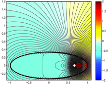
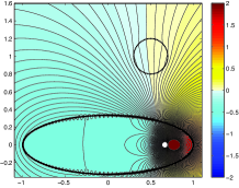
(a)	(b)

Figure 1: Isopotentials without (a) and with (b) a target with $\sigma=5$ and $\varepsilon=0$.

In a previous study [2], we have extracted the GPTs of a target by multistatic measurements using arrays of sources and receptors. These GPTs were then arranged and compared to a dictionary of already known shapes. This study aims at adapting this method to the electro-sensing problem.

2.2 Asymptotic formalism

The first step is to compute the GPTs from the measurements. In this regard, the next result will be useful. Except when mentioned, we will fix in this section the frequency $\omega$, leading to a fixed complex admittivity $k$. We will need the following notation. For a multi-index $\alpha\in\mathbb{N}^{d}$, let $x^{\alpha}=x_{1}^{\alpha_{1}}\ldots x_{d}^{\alpha_{d}},\partial^{\alpha}=\partial_{1}^{\alpha_{1}}\ldots\partial_{d}^{\alpha_{d}},$ with $\partial_{j}=\partial/\partial x_{j}$. Let $G(x)$ be the Green function of the Laplacian in $\mathbb{R}^{d}$ which satisfies $\Delta G=\delta$ (where $\delta$ is the Dirac function at the origin) and is given by

$$G(x)=\left\{\begin{array}[]{ll}\displaystyle\frac{1}{2\pi}\ln|x|,&d=2,\\ \vskip 6.0pt plus 2.0pt minus 2.0pt\cr\displaystyle-\frac{1}{4\pi}\frac{1}{|x|},&d=3.\end{array}\right.$$

We denote the single and double layer potentials of a function $\phi\in L^{2}(\partial\Omega)$ as $\mathcal{S}_{\Omega}[\phi]$ and $\mathcal{D}_{\Omega}[\phi]$, where

$$\mathcal{S}_{\Omega}[\phi](x) :=\int_{\partial\Omega}G(x-y)\phi(y)\,d\sigma(y),\quad x\in\mathbb{R}^{d},$$ (2)

and

$$\mathcal{D}_{\Omega}[\phi](x):=\int_{\partial\Omega}\frac{\partial G}{\partial{\nu(y)}}(x-y)\phi(y)\,d\sigma(y),\quad x\in\mathbb{R}^{d}\setminus\partial\Omega.$$ (3)

We also define the boundary integral operator $\mathcal{K}^{*}_{\Omega}$ on $L^{2}(\partial\Omega)$ by

$$\mathcal{K}_{\Omega}^{*}[\phi](x):=\int_{\partial\Omega}\frac{\partial G}{\partial{\nu(x)}}(x-y)\phi(y)\,d\sigma(y),\quad\phi\in L^{2}(\partial\Omega).$$ (4)

The operator $\mathcal{K}^{*}_{\Omega}$ is called the Neumann-Poincaré operator. We assume that the target is away from the fish, i.e., the distance between the fish and the target is much larger than the target’s characteristic size but smaller than the range of the electrolocation which does not exceed two fish’s body lengths. The following theorem holds.

Theorem 1.

Let us define the function $H:\mathbb{R}^{d}\rightarrow\mathbb{C}$ by

$$H(x)=p(x)+\mathcal{S}_{\Omega}\left[\left.\frac{\partial u}{\partial\nu}\right|_{+}\right]-\xi\mathcal{D}_{\Omega}\left[\left.\frac{\partial u}{\partial\nu}\right|_{+}\right],$$ (5)

where $p$ is the field created by the dipole $f$, i.e., $\Delta p=f$ in $\mathbb{R}^{d}$. Then, for every integer $K\geq 1$, the following expansion holds

$$\begin{array}[]{l}\displaystyle u(x)=H(x)+\delta^{d-2}\sum_{\left|\alpha\right|=1}^{K}\sum_{\left|\beta\right|=1}^{K-\left|\alpha\right|+1}\frac{(-1)^{|\beta|}\delta^{\left|\alpha\right|+\left|\beta\right|}}{\alpha!\beta!}\partial^{\alpha}H(z)\\ \vskip 6.0pt plus 2.0pt minus 2.0pt\cr\qquad\qquad\displaystyle\times M_{\alpha\beta}(\lambda,B)\partial^{\beta}G(x-z)+O(\delta^{d+K}),\end{array}$$ (6)

uniformly for $x\in\partial\Omega$, where $z$ is the location of the target $D$ and

$$M_{\alpha\beta}(\lambda,B):=\int_{\partial B}(\lambda I-\mathcal{K}_{B}^{*})^{-1}[\frac{\partial y^{\alpha}}{\partial\nu}]y^{\beta}\,d\sigma(y)$$

is the generalized polarization tensor (of order $(\alpha,\beta)$) associated with the domain $B$ and the contrast $\lambda=(k+1)/2(k-1)$; see [9]. Here, $\mathcal{K}_{B}^{*}$ is the Neumann-Poincaré operator associated with $B$ and $I$ is the identity operator.

Let us make a few remarks. First, the definition of the GPTs still holds for complex-valued $\lambda$. However, some properties are lost by this change; thus one has to study them more carefully in this situation. Second, the function $H$, which is computed from the boundary measurements, still depends on $\delta$ but this is not important for our present study. Indeed, formula (6) could have been derived with $U$, the background solution in the absence of the target, instead of $H$ and $G_{R}$ - the Green function associated to Robin conditions on $\partial\Omega$ - instead of $G$, but it is much easier to compute $\partial^{\alpha}H(z)$ and $\partial^{\beta}G(x-z)$ once $z$ is known. This leads us to the third remark: the location $z$ is supposed to be known from the algorithm developed in [1]. Electrolocation algorithms are either based on a space-frequency approach in the case of multifrequency measurements or on the fish’s movement if only one frequency is used [1, 21]. Finally, it is worth mentioning that the knowledge of $M_{\alpha\beta}(\lambda,B)$ for all $\alpha,\beta\in\mathbb{N}^{d}$ determines uniquely $B$ and $\lambda$ [7, 8]. Moreover, the following scaling relation holds:

$$M_{\alpha\beta}(\lambda,\delta B)=\delta^{d-2+|\alpha|+|\beta|}M_{\alpha\beta}(\lambda,B).$$

We will follow the proof of [8, Theorem 4.8]. In a first step, let us show the following formula.

Lemma 2.

For $x\in\mathbb{R}^{d}$,

$$u(x)=H(x)+\mathcal{S}_{D}(\lambda I-\mathcal{K}_{D}^{*})^{-1}\left[\left.\frac{\partial H}{\partial\nu}\right|_{\partial D}\right](x),$$ (7)

where $\nu$ is the outward normal unit vector at $\partial D$ and $\mathcal{S}_{D}$ and $\mathcal{K}_{D}^{*}$ are respectively defined by (2) and (4) with $\Omega$ replaced with $D$.

Proof.

In [1, Section 4.1.2], it is shown that

$$u(x)=p(x)+\mathcal{S}_{\Omega}[\psi](x)+\mathcal{D}_{\Omega}[\phi](x)+\mathcal{S}_{D}[\phi](x),$$

where the functions $\psi$, $\phi\in L^{2}(\partial\Omega)$ and $\phi\in L^{2}(\partial D)$ verify the following system

$$\left\{\begin{aligned} \phi&=-\xi\psi&\,\,\mbox{on }\partial\Omega,\\ \left(\frac{I}{2}-\mathcal{K}_{\Omega}^{*}+\xi\frac{\partial\mathcal{D}_{\Omega}}{\partial\nu}\right)[\psi]-\frac{\partial}{\partial\nu}(\mathcal{S}_{D}[\phi])&=\frac{\partial p}{\partial\nu}&\,\,\mbox{on }\partial\Omega,\\ -\frac{\partial}{\partial\nu}(\mathcal{S}_{\Omega}[\psi])+\xi\frac{\partial}{\partial\nu}(\mathcal{D}_{\Omega}[\psi])+(\lambda I-\mathcal{K}_{D}^{*})&[\phi]=\frac{\partial p}{\partial\nu}&\,\mbox{on }\partial D.\end{aligned}\right.$$

The third line gives us

$$\phi=(\lambda I-\mathcal{K}_{D}^{*})^{-1}\left[\left.\frac{\partial H}{\partial\nu}\right|_{\partial D}\right],$$

and the jump formulas for the single and double layer potentials [9, Theorem 2.17] give us

$$\psi=\frac{\partial u}{\partial\nu}\bigg{|}_{+}\quad\mbox{ and }\phi=-u|_{+}+u|_{-},$$

so that, from the boundary conditions of the system (1), we obtain $p+\mathcal{S}_{\Omega}[\psi]+\mathcal{D}_{\Omega}[\phi]=H$ and the lemma is proved. $\Box$

We can now prove Theorem 1, using the arguments in [8, pp. 72-73]. Starting with formula (7), the proof relies on a Taylor expansion of $H$ and the Green function involved in the single layer potential. Indeed, denoting

$$H_{K}(x)=\sum_{\left|\alpha\right|=0}^{K}\frac{1}{\alpha!}\partial^{\alpha}H(z)(x-z)^{\alpha},$$

a Taylor expansion gives us

$$\left\|\frac{\partial H}{\partial\nu}-\frac{\partial H_{K}}{\partial\nu}\right\|_{L^{2}(\partial D)}\leq C\delta^{K}\left|\partial D\right|^{1/2},$$

and from [8, Formula (4.10)], we have for any $h\in L^{2}(\partial D)$ such that $\int_{\partial D}h=0$:

$$\forall x\in\partial\Omega,\,\,\left|\mathcal{S}_{D}(\lambda I-\mathcal{K}_{D}^{*})^{-1}[h](x)\right|\leq C\delta\left|\partial D\right|^{1/2}\left\|h\right\|_{L^{2}(\partial D)}.$$

Hence, using the fact that $\left|\partial D\right|=\delta^{d-1}\left|\partial B\right|$, we obtain

$$\begin{array}[]{l}\displaystyle\left\|\mathcal{S}_{D}(\lambda I-\mathcal{K}_{D}^{*})^{-1}\left[\frac{\partial H}{\partial\nu}-\frac{\partial H_{K}}{\partial\nu}\right]\right\|_{L^{\infty}(\partial\Omega)}\\ \vskip 6.0pt plus 2.0pt minus 2.0pt\cr\qquad\leq\displaystyle C\delta\left|\partial D\right|^{1/2}\left\|\frac{\partial H}{\partial\nu}-\frac{\partial H_{K}}{\partial\nu}\right\|_{L^{2}(\partial D)}\leq C\delta^{d+K}.\end{array}$$

Plugging this inequality into (7) enables us to write, for $x\in\partial\Omega$,

$$u(x)=H(x)+\mathcal{S}_{D}(\lambda I-\mathcal{K}_{D}^{*})^{-1}\left[\frac{\partial H_{K}}{\partial\nu}\right](x)+O(\delta^{d+K}).$$

By a change of variables $y^{\prime}=(y-z)/\delta$, denoting $\phi_{\alpha}(y^{\prime})=(\lambda I-\mathcal{K}_{B}^{*})^{-1}[\nu\cdot\nabla w^{\alpha}](y^{\prime})$ for $y^{\prime}\in\partial B$ (where $\nu$ is here the outward normal unit vector to $\partial B$), we have (see for example the arguments in [5, Section 3])

$$\begin{array}[]{l}\displaystyle u(x)-H(x)=\sum_{\left|\alpha\right|=0}^{K}\frac{1}{\alpha!}\partial^{\alpha}H(z)\delta^{\left|\alpha\right|+d-2}\\ \vskip 6.0pt plus 2.0pt minus 2.0pt\cr\qquad\qquad\displaystyle\times\int_{\partial B}G(x-z-\delta y^{\prime})\phi_{\alpha}(y^{\prime})d\sigma(y)+O(\delta^{d+K}).\end{array}$$

We can now conclude by injecting a Taylor expansion of the Green function

$$G(x-z-\delta y)=\sum_{\left|\beta\right|=0}^{\infty}\frac{(-\delta)^{\left|\beta\right|}}{\beta!}\partial^{\beta}G(x-z)y^{\beta},$$

in the integrand, giving

$$\begin{array}[]{l}\displaystyle u(x)-H(x)=\delta^{d-2}\sum_{\left|\alpha\right|=0}^{K}\sum_{\left|\beta\right|=0}^{K-\left|\alpha\right|+1}\frac{(-1)^{|\beta|}\delta^{\left|\alpha\right|+\left|\beta\right|}}{\alpha!\beta!}\partial^{\alpha}H(z)\\ \vskip 6.0pt plus 2.0pt minus 2.0pt\cr\qquad\qquad\displaystyle\times\partial^{\beta}G(x-z)\int_{\partial B}y^{\beta}\phi_{\alpha}(y)d\sigma(y)+O(\delta^{d+K}).\end{array}$$

The last term is $M_{\alpha\beta}(\lambda,B)$ by definition [9]; it then suffices to show that the terms with $\left|\alpha\right|=0$ or $\left|\beta\right|=0$ vanish, which is the case because $\int_{\partial B}\phi_{\alpha}=0$ and $\phi_{\alpha}=0$ if $\left|\alpha\right|=0$. Thus, Theorem 1 is proved. $\Box$

2.3 Data acquisition and reduction

Let us suppose that the fish is moving, and let us take a sample of $S\in\mathbb{N}^{*}$ different positions $\left(\Omega_{s}\right)_{1\leq s\leq S}$. This gives us $2S$ different functions $\left(u_{s}\right)_{1\leq s\leq S}$ and $\left(H_{s}\right)_{1\leq s\leq S}$, leading us to the following data matrix

$$\mathbb{Q}:=\left(Q_{sr}\right)_{1\leq s\leq S,1\leq r\leq R}:=\left(u_{s}(x_{r}^{(s)})-H_{s}(x_{r}^{(s)})\right)_{1\leq s\leq S,1\leq r\leq R},$$ (8)

where $(x_{r}^{(s)}\in\partial\Omega_{s})_{1\leq r\leq R}$ are the receptors of the fish being in the $s^{\mbox{th}}$ position. The choices of indices are motivated by the fact that the different positions play the role of sources.

The goal of this subsection is to simplify this data set in order to extract the GPTs (precisely, the contracted GPTs as it will be seen below). Indeed, from (6), one has

$$\begin{array}[]{l}\displaystyle Q_{sr}=\delta^{d-2}\sum_{\left|\alpha\right|=1}^{K}\sum_{\left|\beta\right|=1}^{K-\left|\alpha\right|+1}(-1)^{|\beta|}\frac{\delta^{\left|\alpha\right|+\left|\beta\right|}}{\alpha!\beta!}\partial^{\alpha}H_{s}(z)\\ \vskip 6.0pt plus 2.0pt minus 2.0pt\cr\qquad\qquad\displaystyle\times M_{\alpha\beta}(\lambda,B)\partial^{\beta}G(x^{(s)}_{r}-z)+O(\delta^{d+K}).\end{array}$$ (9)

As in [2], we will express this formula in terms of contracted GPTs (CGPTs), when the dimension of the space is $d=2$. Let us first recall the definitions of these contracted GPTs. For a target $B$ with contrast ratio $\lambda$, knowing the GPTs $M_{\alpha\beta}(\lambda,B)$ for all indices $\alpha$ and $\beta$ such that $\left|\alpha\right|=m$ and $\left|\beta\right|=n$ leads us to construct the following combinations, called CGPTs,

$$\begin{array}[]{l}\displaystyle M_{mn}^{cc}=\sum_{|\alpha|=m}\sum_{|\beta|=n}a_{\alpha}^{m}a_{\beta}^{n}M_{\alpha\beta},\\ \vskip 6.0pt plus 2.0pt minus 2.0pt\cr\displaystyle M_{mn}^{cs}=\sum_{|\alpha|=m}\sum_{|\beta|=n}a_{\alpha}^{m}b_{\beta}^{n}M_{\alpha\beta},\\ \vskip 6.0pt plus 2.0pt minus 2.0pt\cr\displaystyle M_{mn}^{sc}=\sum_{\left|\alpha\right|=m}\sum_{\left|\beta\right|=n}b_{\alpha}^{m}a_{\beta}^{n}M_{\alpha\beta},\\ \vskip 6.0pt plus 2.0pt minus 2.0pt\cr\displaystyle M_{mn}^{ss}=\sum_{\left|\alpha\right|=m}\sum_{\left|\beta\right|=n}b_{\alpha}^{m}b_{\beta}^{n}M_{\alpha\beta},\end{array}$$

where the real numbers $a_{\alpha}^{m}$ and $b_{\beta}^{m}$ are defined by the following relation

$$(x_{1}+ix_{2})^{m}=\sum_{\left|\alpha\right|=m}a_{\alpha}^{m}x^{\alpha}+i\sum_{\left|\beta\right|=m}b_{\beta}^{m}x^{\beta}.$$

In the polar coordinates, $x=r_{x}e^{i\theta_{x}}$, these coefficients also verify the following characterization

$$\sum_{\left|\alpha\right|=m}a_{\alpha}^{m}x^{\alpha}=r_{x}^{m}\cos m\theta_{x}\mbox{ and }\sum_{\left|\beta\right|=m}b_{\beta}^{m}x^{\beta}=r_{x}^{m}\sin m\theta_{x}.$$

This enables us to show [2, Appendix A.2] that

$$\frac{(-1)^{|\alpha|}}{\alpha!}\partial^{\alpha}G(x)=\frac{-1}{2\pi\left|\alpha\right|}\left(a_{\alpha}^{\left|\alpha\right|}\frac{\cos\left|\alpha\right|\theta_{x}}{r_{x}^{\left|\alpha\right|}}+b_{\alpha}^{\left|\alpha\right|}\frac{\sin\left|\alpha\right|\theta_{x}}{r_{x}^{\left|\alpha\right|}}\right).$$ (10)

From the definition of $H$, and with the help of the previous formula, one can prove the following lemma.

Lemma 3.

Let the source $f$ be a dipole of moment $\mathbf{p}_{s}$ placed at $z_{s}$:

$$p_{s}(x)=\mathbf{p}_{s}\cdot\nabla G(x-z_{s}),$$ (11)

Then, for any $\alpha\in\mathbb{N}^{2}$, there exist two real numbers $A_{\left|\alpha\right|,s,z}$ and $B_{\left|\alpha\right|,s,z}$ such that

$$\frac{1}{\alpha!}\partial^{\alpha}H_{s}(z)=A_{\left|\alpha\right|,s,z}a_{\alpha}^{\left|\alpha\right|}+B_{\left|\alpha\right|,s,z}b_{\alpha}^{\left|\alpha\right|}.$$

Moreover, $A_{\left|\alpha\right|,s,z}$ and $B_{\left|\alpha\right|,s,z}$ can be expressed in the following way

$$\begin{array}[]{lll}A_{m,s,z}&=&\displaystyle\frac{(-1)^{m}}{2\pi}\mathbf{p}_{s}\cdot\left(\begin{array}[]{c}\phi_{m+1}(z-z_{s})\\ \psi_{m+1}(z-z_{s})\end{array}\right)\\ \vskip 6.0pt plus 2.0pt minus 2.0pt\cr&&\displaystyle-\frac{1}{2\pi m}\int_{\partial\Omega}\left.\frac{\partial u_{s}}{\partial\nu}\right|_{+}(y)\phi_{m}(y-z)d\sigma(y),\\ \vskip 6.0pt plus 2.0pt minus 2.0pt\cr&&\displaystyle-\frac{\xi}{2\pi}\int_{\partial\Omega}\left(\begin{array}[]{c}\phi_{m+1}(y-z)\\ \psi_{m+1}(y-z)\end{array}\right)\cdot\nu_{y}\left.\frac{\partial u_{s}}{\partial\nu}\right|_{+}(y)\,d\sigma(y),\\ \vskip 6.0pt plus 2.0pt minus 2.0pt\cr B_{m,s,z}&=&\displaystyle\frac{(-1)^{m}}{2\pi}\mathbf{p}_{s}\cdot\left(\begin{array}[]{c}\psi_{m+1}(z-z_{s})\\ -\phi_{m+1}(z-z_{s})\end{array}\right)\\ \vskip 6.0pt plus 2.0pt minus 2.0pt\cr&&\displaystyle-\frac{1}{2\pi m}\int_{\partial\Omega}\left.\frac{\partial u_{s}}{\partial\nu}\right|_{+}(y)\psi_{m}(y-z)d\sigma(y)\\ \vskip 6.0pt plus 2.0pt minus 2.0pt\cr&&\displaystyle-\frac{\xi}{2\pi}\int_{\partial\Omega}\left(\begin{array}[]{c}\psi_{m+1}(y-z)\\ -\phi_{m+1}(y-z)\end{array}\right)\cdot\nu_{y}\left.\frac{\partial u_{s}}{\partial\nu}\right|_{+}(y)\,d\sigma(y),\end{array}$$

where the functions $\phi_{m}$ and $\psi_{m}$ are defined for $x\in\mathbb{R}^{2}$, $x=(r_{x},\theta_{x})$ in the polar coordinates, by

$$\phi_{m}(x) =\frac{\cos m\theta_{x}}{r_{x}^{m}},\quad\psi_{m}(x) =\frac{\sin m\theta_{x}}{r_{x}^{m}}.$$

Proof.

Let us fix $\alpha\in\mathbb{N}^{2}$ and define $m=|\alpha|$. Let us recall the definition of $H$, given in (5)

$$H_{s}(x)=p_{s}(x)+\mathcal{S}_{\Omega_{s}}\left[\left.\frac{\partial u_{s}}{\partial\nu}\right|_{+}\right]-\xi\mathcal{D}_{\Omega_{s}}\left[\left.\frac{\partial u_{s}}{\partial\nu}\right|_{+}\right],$$

where $\Delta p_{s}=f_{s}$ in $\mathbb{R}^{2}$. From (11) it follows that

$$\partial^{\alpha}p_{s}(x)=\mathbf{p}_{s}\cdot\nabla\partial^{\alpha}G(x-z_{s}).$$

Hence, (10) yields

$$\begin{array}[]{l}\displaystyle\frac{(-1)^{|\alpha|}}{\alpha!}\partial^{\alpha}p_{s}(z)=\displaystyle a_{\alpha}^{m}\left[\frac{-1}{2\pi m}\mathbf{p}_{s}\cdot\nabla\phi_{m}(z-z_{s})\right]\\ \qquad\qquad\displaystyle+b_{\alpha}^{m}\left[\frac{-1}{2\pi m}\mathbf{p}_{s}\cdot\nabla\psi_{m}(z-z_{s})\right].\end{array}$$

Moreover, we have

$$\nabla\phi_{m} =-m\left(\begin{array}[]{c}\phi_{m+1}\\ \psi_{m+1}\end{array}\right),\quad\nabla\psi_{m} =-m\left(\begin{array}[]{c}\psi_{m+1}\\ -\phi_{m+1}\end{array}\right).$$

In the same manner, from

$$\mathcal{S}_{\Omega_{s}}\left[\left.\frac{\partial u_{s}}{\partial\nu}\right|_{+}\right](x)=\int_{\partial\Omega_{s}}\left.\frac{\partial u_{s}(y)}{\partial\nu}\right|_{+}G(y-x)d\sigma(y),$$

we can deduce

$$\begin{array}[]{l}\displaystyle\frac{1}{\alpha!}\partial^{\alpha}\mathcal{S}_{\Omega_{s}}\left[\left.\frac{\partial u_{s}}{\partial\nu}\right|_{+}\right](z)\\ \vskip 6.0pt plus 2.0pt minus 2.0pt\cr\displaystyle=\frac{1}{\alpha!}\int_{\partial\Omega_{s}}\left.\frac{\partial u_{s}}{\partial\nu}\right|_{+}(y)(-1)^{|\alpha|}\partial^{\alpha}G(y-z)d\sigma(y)\\ \vskip 6.0pt plus 2.0pt minus 2.0pt\cr\displaystyle=a_{\alpha}^{m}\left(\int_{\partial\Omega_{s}}\frac{-1}{2\pi m}\left.\frac{\partial u_{s}}{\partial\nu}\right|_{+}(y)\frac{\cos m\theta_{y-z}}{r_{y-z}^{m}}d\sigma(y)\right)\\ \vskip 6.0pt plus 2.0pt minus 2.0pt\cr\displaystyle+b_{\alpha}^{m}\left(\int_{\partial\Omega_{s}}\frac{-1}{2\pi m}\left.\frac{\partial u_{s}}{\partial\nu}\right|_{+}(y)\frac{\sin m\theta_{y-z}}{r_{y-z}^{m}}d\sigma(y)\right).\end{array}$$

Combining those two equations leads us to the desired result. $\Box$

From (9), the data matrix is then expressed as follows

$$Q_{rs} =\sum_{\left|\alpha\right|+\left|\beta\right|=1}^{K+1}\left(A_{\left|\alpha\right|,s,z}a_{\alpha}^{\left|\alpha\right|}+B_{\left|\alpha\right|,s,z}b_{\alpha}^{\left|\alpha\right|}\right)$$ (12)

$$\times M_{\alpha\beta}(\lambda,\delta B)\frac{-a_{\beta}^{\left|\beta\right|}\cos\left|\beta\right|\theta_{x_{r}^{(s)}-z}-b_{\beta}^{\left|\beta\right|}\sin\left|\beta\right|\theta_{x_{r}^{(s)}-z}}{2\pi\left|\beta\right|r_{x_{r}^{(s)}-z}^{\left|\beta\right|}}$$

$$+O(\delta^{K+2})$$

$$=\sum_{m+n=1}^{K+1}\underbrace{\left(\begin{array}[]{cc}A_{m,s,z}&B_{m,s,z}\end{array}\right)}_{\mathbf{S}_{sm}}\underbrace{\left(\begin{array}[]{cc}M_{mn}^{cc}&M_{mn}^{cs}\\ M_{mn}^{sc}&M_{mn}^{ss}\end{array}\right)}_{\mathbf{M}_{mn}}$$

$$\times\underbrace{\left(\begin{array}[]{c}\cos n\theta_{x_{r}^{(s)}-z}\\ \sin n\theta_{x_{r}^{(s)}-z}\end{array}\right)\frac{-1}{2\pi nr_{x_{r}^{(s)}-z}^{n}}}_{\mathbf{G^{(s)}}_{nr}}+\underbrace{O(\delta^{K+2})}_{{E}_{rs}}.$$

Thus, defining the following matrices

$$\mathbb{M}=\left(\begin{array}[]{cccc}\mathbf{M}_{11}&\mathbf{M}_{12}&\ldots&\mathbf{M}_{1K}\\ \mathbf{M}_{21}&&\iddots&0\\ \vdots&\iddots&\iddots&\vdots\\ \mathbf{M}_{K1}&0&\ldots&0\end{array}\right),\,\,\mathbb{E}=\left({E}_{rs}\right)_{1\leq r\leq R,1\leq s\leq S},$$

the problem is to recover the matrix $\mathbb{M}$ knowing the matrix

$$\mathbb{Q}=\mathcal{L}(\mathbb{M})+\mathbb{E},$$

where $\mathcal{L}$ is the linear operator defined by (12).

Therefore, the CGPTs of the target $D$ can be reconstructed as the least-squares solution of the above linear system, i.e.,

$$\widehat{\mathbb{M}}=\underset{\mathbb{M}\perp\mathrm{ker}(\mathcal{L})}{\mbox{argmin}}\|\mathbb{Q}-\mathcal{L}(\mathbb{M})\|^{2}_{F},$$ (13)

where $\mathrm{ker}(\mathcal{L})$ denotes the kernel of $\mathcal{L}$ and $\|\cdot\|_{F}$ denotes the Frobenius norm of matrices [2].

Let us remark that, in the case of multifrequency measurements $(\omega_{1},\ldots,\omega_{F})$, we can reconstruct $\left(\widehat{\mathbb{M}}^{(f)}\right)_{1\leq f\leq F}$ from $\left(\mathbb{Q}^{(f)}\right)_{1\leq f\leq F}$ analogously.

It is worth mentioning that the location of the target detected by the fish may be different from the true one. Moreover, the target may be rotated and hence, the reconstructed CGPTs correspond to a translated, scaled, and rotated target $B$. In order to recognize the shape $B$, it is therefore fundamental for the recognition procedure to have size invariance, rotational invariance, and translational invariance. This could be related to the behavioral experiments that have shown that weakly electric fish categorize targets according to their shapes but not according to sizes, locations, or orientations [34].

3 Recognition and classification

Depending on whether we consider multifrequency measurements or not, we will not identify the CGPTs in the same way.

3.1 Fixed frequency setting: shape descriptor based classification

In [2], an algorithm based on shape descriptors was developed for the recognition of a target in a more classical electrical sensing setup, (i.e., multiple sources/receptors placed on the surface of a disk). In this paper, we apply this algorithm in the context of electro-sensing.

We recall here the concept and properties of shape descriptors in two dimensions [2]. For a double index $mn$, with $m,n=1,2,\ldots$, we introduce the following complex combinations, $\mathbf{N}^{(1)}=(\mathcal{N}^{(1)}_{mn})_{m,n},\mathbf{N}^{(2)}=(\mathcal{N}^{(2)}_{mn})_{m,n}$, of CGPTs:

$$\mathcal{N}^{(1)}_{mn}(\lambda,D) =(M^{cc}_{mn}-M^{ss}_{mn})+i(M^{cs}_{mn}+M^{sc}_{mn}),$$ (14)

$$\mathcal{N}^{(2)}_{mn}(\lambda,D) =(M^{cc}_{mn}+M^{ss}_{mn})+i(M^{cs}_{mn}-M^{sc}_{mn}).$$

Let

$$u=\frac{\mathcal{N}^{(2)}_{12}(D)}{2\mathcal{N}^{(2)}_{11}(D)},\quad T_{-u}D=\{x-u,x\in D\}.$$

We define the following quantities which are translation invariant:

$${\mathbf{\mathcal{J}^{(1)}}}(D) =\mathbf{N}^{(1)}(T_{-u}D)=\mathbf{C}^{-u}\mathbf{N}^{(1)}(D)(\mathbf{C}^{-u})^{t},$$ (15)

$${\mathbf{\mathcal{J}^{(2)}}}(D) =\mathbf{N}^{(2)}(T_{-u}D)=\overline{\mathbf{C}^{-u}}\mathbf{N}^{(2)}(D)(\mathbf{C}^{-u})^{t},$$ (16)

with $t$ being the transpose and the matrix $\mathbf{C}^{-u}$ being a lower triangular matrix with the $m,n$-th entry given by

$$\mathbf{C}^{-u}_{mn}=\binom{m}{n}(-u)^{m-n}.$$

From ${\mathbf{\mathcal{J}^{(1)}}}(D)=(\mathcal{J}^{(1)}_{mm}(D))_{m,n}$ and ${\mathbf{\mathcal{J}^{(2)}}}(D)=(\mathcal{J}^{(2)}_{mm}(D))_{m,n}$, we define, for any indices $m,n$, the scaling invariant quantities:

$$\mathcal{S}^{(j)}_{mn}(D)=\frac{\mathcal{J}^{(j)}_{mn}(D)}{\left(\mathcal{J}^{(2)}_{mm}(D)\mathcal{J}^{(2)}_{nn}(D)\right)^{1/2}},\quad j=1,2.$$ (17)

Finally, we introduce the CGPT-based shape descriptors ${\mathbf{\mathcal{I}^{(1)}}}=(\mathcal{I}^{(1)}_{mn})_{m,n}$ and ${\mathbf{\mathcal{I}^{(2)}}}=(\mathcal{I}^{(2)}_{mn})_{m,n}$:

$$\mathcal{I}^{(1)}_{mn}(D)=|\mathcal{S}^{(1)}_{mn}(D)|,\qquad\ \mathcal{I}^{(2)}_{mn}(D)=|\mathcal{S}^{(2)}_{mn}(D)|,$$ (18)

where $|\cdot|$ denotes the modulus of a complex number. Constructed in this way, ${\mathbf{\mathcal{I}^{(1)}}}$ and ${\mathbf{\mathcal{I}^{(2)}}}$ are invariant under translation, rotation, and scaling. Only shape descriptors of order $2$, i.e., for $m,n=1,2$ will be used in the sequel. Shape descriptors in three dimensions were derived in [4].

3.2 Multifrequency setting: Spectral induced polarization based classification

When multiple frequencies are involved, we can use the shape descriptors $\mathcal{I}^{(1)}_{mn}(D)$ and $\mathcal{I}^{(2)}_{mn}(D)$ at frequencies $\omega_{1},\ldots,\omega_{F}$ to enhance the stability of the classification. However, as it will be shown later, this does not yield a very stable classification procedure.

Here we rather focus on the first-order polarization tensor (PT), that is, the $2\times 2$ complex matrix $\mathcal{M}^{(f)}(D)$ associated with the target $D$ and frequency $f$:

$$\mathcal{M}^{(f)}(D):=\int_{\partial D}\bigg{(}\frac{\sigma+1+i\omega_{f}\varepsilon}{2(\sigma-1+i\omega_{f}\varepsilon)}I-\mathcal{K}_{D}^{*}\bigg{)}^{-1}[\nu]y\,d\sigma(y),$$

for $f=1,\ldots,F$. We will show that they are sufficient to identify efficiently the targets. Note that it is not possible to compute the shape descriptors $\mathcal{I}^{(1)}_{mn}(D)$ and $\mathcal{I}^{(2)}_{mn}(D)$ based only on first-order PT, because they require at least second-order polarization tensors. This limits the use of shape descriptors in the limited-view case where the reconstruction of higher-order GPTs is not accurate [3].

Here we use the spectral content of the first-order PTs for recognition. We have the following properties [9].

Proposition 4.

For any scaling $\delta>0$, rotation angle $\theta\in\mathbb{R}$ and translation vector $z\in\mathbb{R}^{2}$, let us denote

$$D=z+\delta R_{\theta}B:=\left\{x=z+\delta R_{\theta}u,\,\,u\in B\right\},$$

where

$$R_{\theta}:=\left(\begin{array}[]{cc}\cos\theta&-\sin\theta\\ \sin\theta&\cos\theta\end{array}\right),$$

is the rotation matrix of angle $\theta$. Then,

$$\mathcal{M}^{(f)}(D)=\delta^{2}R_{\theta}\mathcal{M}^{(f)}(B)R_{\theta}^{T}.$$ (19)

Hence, if we denote by $\tau_{1}^{(f)}(D)$ and $\tau_{2}^{(f)}(D)$ the singular values of $\mathcal{M}^{(f)}(D)$, we obtain

$$\forall j\in\{1,2\},\,\,\tau_{j}^{(f)}(D)=\delta^{2}\tau_{j}^{(f)}(B).$$

This gives an idea for two algorithms:

1. The first one, matching the singular values of all the first-order PT $\left(\mathcal{M}^{(f)}\right)_{1\leq f\leq F}$, would be dependent of the characteristic scale $\delta$ of the targets in the dictionary;

2. The second one, independent of the scale of the target, would match the following quantities

   $$\mu_{j}^{(f)}=\frac{\tau_{j}^{(f)}}{\tau_{j}^{(F)}},$$ (20)

   for $j=1,2$ and $f=1,\ldots,F-1$.

Some comments are in order. First, the reason why we consider the first one, even if it is scale-dependent, is because it is far more stable. Also, in some biological experiments, two targets of different scales are considered as different [35]. A question raised was then: how is it possible to discriminate between a nearby small target and an extended one situated far away? With the second algorithm, we have an answer. The last remark concerns equation (20). We could have also considered other scale-dependent ratios, such as

$$\frac{\tau_{j}^{(f)}}{\tau_{j}^{(1)}}\mbox{ or }\frac{\tau_{j}^{(f)}}{\sum_{f^{\prime}=1}^{F}\tau_{j}^{(f^{\prime})}},$$

but since $\tau_{j}^{(F)}$ happens to be the largest one (the frequencies are sorted in increasing order), it is more stable to consider (20). It is worth mentioning that if there exists an integer $p>2$ such that $R_{2\pi/p}D=D$, then $\mathcal{M}^{(f)}(D)$ is proportional to identity.

3.3 Background field elimination

We can also improve stability of reconstruction by eliminating the background field. Let us denote by $U(x)$ the background electric field (i.e., the solution of (1) with $k=1$). In [1, Proposition 2], we have proved the following formula:

$$\mathcal{P}_{\Omega}\left(\left.\frac{\partial u_{f}}{\partial\nu}\right|_{+}-\left.\frac{\partial U}{\partial\nu}\right|_{+}\right)\approx\nabla U(z)^{T}\mathcal{M}^{(f)}(D)\nabla_{z}\left(\frac{\partial G}{\partial\nu_{x}}\right),$$ (21)

where $u_{f}$ is $u$ associated with the $f^{\textrm{th}}$ frequency, $\mathcal{M}^{(f)}(D)$ is the first-order polarization tensor at the $f^{\textrm{th}}$ frequency, and $\mathcal{P}_{\Omega}$ is the (real-valued) postprocessing operator given by

$$\mathcal{P}_{\Omega}:=\frac{1}{2}I-\mathcal{K}_{\Omega}^{*}-\xi\frac{\partial\mathcal{D}_{\Omega}}{\partial\nu},$$

with $\mathcal{D}_{\Omega}$ and $\mathcal{K}_{\Omega}^{*}$ being defined by (3) and (4); see [1]. Hence, if the emitted signal $U$ is real-valued, then taking the imaginary part leads us to

$$\mathcal{P}_{\Omega}\left[\Im m\,\left(\left.\frac{\partial u_{f}}{\partial\nu}\right|_{+}\right)\right]\approx\nabla U(z)^{T}\Im m\,\mathcal{M}^{(f)}(D)\nabla_{z}\left(\frac{\partial G}{\partial\nu_{x}}\right).$$ (22)

Note that in biological sciences, the restriction on $U$ to be real is justified since the permittivities of water and the fish are negligible [1]. Now, from (22), we can extract $\Im m\,\mathcal{M}^{(f)}(D)$ by solving a least-squares problem similar to (13). Then, we have the singular values of the imaginary part of $\mathcal{M}^{(f)}(D)$, which would be sufficient for shape recognition and classification. The goal of this procedure is to get rid off the computation of $\partial U/\partial\nu$ in (21), which is supposed to be performed numerically in real-world applications, thus subject to errors. Note that the postprocessing operator ${\mathcal{P}}_{\Omega}$ makes the data independent of the shape of the fish’s body.

Because of the following relation which follows from (19)

$$\mathcal{M}^{(f)}(D)=O(\delta^{2}\mathcal{M}^{(f)}(B)),$$

taking the imaginary part would lead us to only compute $\nabla U(z)$ in (22) and hence, the error made here would be modulated by a factor of order $\delta^{2}$.

4 Numerical illustrations

In this section, we illustrate the performance of the algorithms developed in the previous section. We use the CGPTs obtained in order to classify the targets. We present an example with fixed frequency, and another with multifrequency measurements. As it will be seen, the latter does not lead us to a significantly more stable classification in the presence of noise or for limited aperture. The errors in the reconstruction of the high-order polarization tensors due to measurement noise or the limited-view aspect deteriorate the stability of the proposed algorithm. However, when, at multiple frequencies, only the first-order polarization tensor is used, we arrive at a very robust and efficient classification procedure.

For the sake of clarity, and due to the large numbers of computations performed, the results are presented in the appendix.

4.1 Setup and methods

We describe the dictionary as well as the measurement systems. We consider two different shapes for the fish: ellipses and twisted ellipses. Note that this variety of shapes exists in nature. On the one hand, twisted ellipses would represent electric eels (Electrophorus electricus), whereas on the other hand straight ellipses would look like Apteronotids [25]. This simplified representation shows that the principle of our algorithms can be generalized to any kind of fish’s shape (hence modeling, for example, electro-sensing for Mormyrids as well). It also enhances the fact that, for bio-inspired engineering applications, the shape of the robot is not determining. Moreover, as we will see later, our simplified representation is a good model to tackle aperture issues.

4.1.1 Dictionary

The dictionary $\mathcal{D}$ that we consider is composed by 8 different targets: a disk, an ellipse, the letter ’A’, the letter ’E’, a rectangle, a square, a triangle, and an ellipse with different electrical parameters (see Fig. 2). Indeed, all the other targets have conductivity $\sigma=2$ and permittivity $\varepsilon=1$ whereas the last one has conductivity $\sigma=5$ and permittivity $\varepsilon=2$. Except when mentioned, the characteristic size of the target will not matter, and will be fixed to be of order $1$.

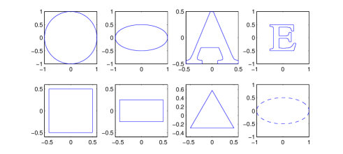
Figure 2: The 8 elements of the dictionary. The dotted lines indicate a target with different electrical parameters.

4.1.2 Measurements

In each numerical experiment, one target of the dictionary is placed at the origin, while the fish swims around it. As it has been mentioned, we consider two different shapes for the fish’s body: ellipses and twisted ellipses. The measured data is built taking $20$ positions of the fish around the target (see Fig. 3).

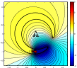
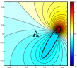
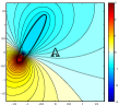
Figure 3: Two different kinds of experiences involve (on the top) a twisted-ellipse shape or (on the bottom) ellipse shape. The real part of the electric field is plotted, for $3$ (out of $20$) positions that the fish takes around the target (placed at the origin).

In Fig. 4, a smaller aperture than the one in Fig. 3 is considered.

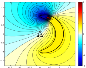
Figure 4: A fish having the shape of a twisted ellipse with a smaller aperture than in Fig. 3.

The typical size of the target is $\delta=0.3$ while the fish is turning around a disk of radius $R=1$; the twisted ellipse’s semi-axes are $a=1.8$ and $b=0.2$ while the straight ellipse’s semi axis are $a=1$ and $b=0.2$. The effective thickness of the skin is set at $\xi=0$. The fish has $2^{7}$ receptors uniformly distributed on its skin, and the electric organ emits $F=10$ frequencies, equally distributed from $\omega_{0}:=1$ to $F\omega_{0}$. Again, we refer to [1] for nondimensionalization of the underlying model equations with proper quantities and realistic values.

4.1.3 Classification

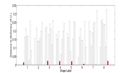
Figure 5: Results of the matching with the dictionary (differences between shape descriptors), when the fish is a twisted ellipse. The red bar represents the bar of the target being identified. In the $x$-coordinates, 1 stands for the disk, 2 for the ellipse, 3 for the letter A, 4 for the letter E, 5 for the square, 6 for the rectangle, 7 for the triangle and 8 for the ellipse with different electrical parameters. In the $y$-coordinates, the distance between the shape descriptor of the target - computed from measurements - and the shape descriptors of the dictionary.

The recognition process is as follows. When measurements are acquired, we perform least-square reconstruction of the (first- or second-order) CGPT of the targets. From this CGPT, we compute quantities of interest $q$ (i.e. Shape Descriptors or singular values or ratios of singular values). Then, for each element $n$ in the dictionary $\mathcal{D}$, we compute ${\left\|q-q_{n}\right\|}$, where $q_{n}$ is the - pre-computed - quantity of interest for the $n$th shape. This leads us to charts such as the ones presented in Figs. 5, 6, and 7.

• Framework for algorithms of multifrequency classification:

  1:  Input: the quantities of interest $\left(q^{(f)}\right)_{1\leq f\leq F}$ calculated from the measurement of an unknown shape $D$;

  2:  for $B_{n}\in\mathcal{D}$ do

  3:     $e_{n}\leftarrow\sum_{1\leq f\leq F}\|q(B_{n})^{(f)}-q^{(f)}\|^{2}$ where $\left(q(B_{n})^{(f)}\right)_{1\leq f\leq F}$ is the same type of quantities of interest of the shape $B_{n}$;

  4:     $n\leftarrow n+1$;

  5:  end for

  6:  Output: the true dictionary element $n^{*}\leftarrow\mbox{argmin}_{n}e_{n}$.

4.1.4 Stability analysis

First, let us explain what kind of noise is considered. We will add a random matrix (with Gaussian entries) to the data matrix $\mathbb{Q}$ defined in (8). More precisely, we will consider

$$\tilde{\mathbb{Q}}:=\mathbb{Q}+\varepsilon\mbox{$\mathbb{W}$},$$

where $\mathbb{W}$ is a $S\times R$ matrix whose coefficients follow a Gaussian distribution with mean $0$ and variance $1$. The real number $\varepsilon$ is the strength of the noise, and will be given in percentage of the fluctuations of $\mathbb{Q}$, (i.e., $\max_{s,r}Q_{sr}-\min_{s,r}Q_{sr}$). The recognition procedure remains the same.

Stability analysis was then carried out empirically: for each noise level, we performed $N_{\textrm{stabil}}$ independent recognition process (with $N_{\textrm{stabil}}$ being precised for each experiment), and computed the ratio of good detection. The computation ends when we reach the threshold of $12.5\%$ probability of detection that corresponds to a uniform random choice of the object. This gives us Figs. 8 to 15.

4.2 Results and discussion

In this subsection, we compare the respective stability of our algorithms. Due to the large number of situations and computations, only significant figures were plotted, giving the following classification of recognition processes, according to their range of application.

4.2.1 Fixed frequency setting: shape descriptors

If only one frequency is accessible for the measurements, then the only algorithm possible is classification based on shape descriptors. Indeed, first-order PTs are not enough to discriminate between objects. However, the use of shape descriptors is limited to the twisted-ellipse case with nearly full aperture (see Figs. 6 and  7, where some targets are not recognized, such as the ellipse in Fig. 6 or the disk in Fig. 7). Moreover, its stability with respect to measurement noise is quite poor (see Fig. 8).

4.2.2 Multifrequency setting: spectral content of PTs

In the case of multifrequency measurements, shape descriptors do not increase their stability enough compared to singular values (see Fig. 9). Hence, it is better to use singular values of the PTs (see Figs. 10 to 13). One can see that:

• considering all singular values (Figs. 10 and 11) is much more stable than considering ratios of singular values (Figs. 12 and 13);

• the aperture does not change very much the stability.

In this regard, the most stable algorithm is to recognize all singular values when the fish is a twisted ellipse (Fig. 10), leading us to a probability of detection superior to $90\%$ with noise level of $125\%$. This is a huge gap when compared to the recognition process with shape descriptors, allowing only a few percents of noise. Note that the noise level is computed with respect to the perturbation in the measurements $\mathbb{Q}$ given by (8), which is of order of the target volume, see (9). Hence, a noise level of $125\%$ remains small compared to the actual transdermal potential $u$.

4.2.3 Background field elimination

We can see in Figs. 14 and 15 that taking the imaginary part of the measurements in order to avoid the computation of the background field does not significantly decrease the stability of the reconstruction based on spectral content. Since the reconstruction of CGPTs is very fast, the background field elimination technique would yield to real-time imaging.

5 Concluding remarks

In this paper, we have successfully exhibited the physical mechanism underlying shape recognition and classification in active electrolocation. We have shown that extracting generalized polarization tensors from the data and comparing invariants with those of learned elements in a dictionary yields a classification procedure with a good performance in the full-view case and with moderate measurement noise level. However, this shape descriptor based classification is instable in the limited-view case and for higher noise level. When measurements at multiple frequencies are used, the stability of our classification approach is significantly improved by using phase shifts and keeping only the first-order polarization tensor. The resulting spectral induced polarization based classification is very robust.

Our results open the door for the application of the extended Kalman filter developed in [3] to show the feasibility of a tracking of both location and orientation of a target from perturbations of the electric field on the skin surface of the fish. It also remains to understand to what extent the spectral induced polarization approach could help us retrieve the electric parameters of the target or locate and recognize multiple targets.

In this appendix, we numerically illustrate the main findings in this paper and show the potential of electro-sensing for shape recognition and classification.

Figure 6: Same results as in 5, with an ellipse-shaped fish.

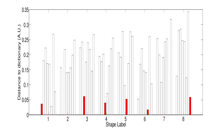
Figure 7: Results of the matching with the dictionary for a twisted ellipse shaped fish with smaller aperture (see Fig. 4).

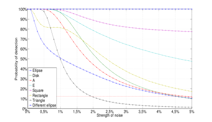
Figure 8: Stability of classification based on Shape Descriptors, when the fish is a twisted ellipse. Here, only one frequency (the smallest one) is considered. The threshold of $12.5\%$ that corresponds to a randomly chosen target is represented in red dotted line. Here, $N_{\textrm{stabil}}=10^{5}$.

Figure 9: Stability of classification based on multifrequency Shape Descriptors, when the fish is a twisted ellipse. Here, $N_{\textrm{stabil}}=5.10^{4}$.

Figure 10: Stability of classification based on differences between all singular values of PTs, when the fish is a twisted ellipse. The characteristic size of the target is supposed to be known. Here, $N_{\textrm{stabil}}=5.10^{4}$.

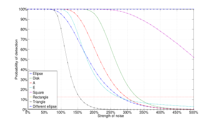
Figure 11: Stability of classification based on differences between all singular values of PTs, when the fish is a straight ellipse. The characteristic size of the target is supposed to be known. Here, $N_{\textrm{stabil}}=5.10^{4}$.

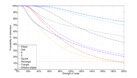
Figure 12: Stability of classification based on differences between ratios of singular values, when the fish is a twisted ellipse. Here, $N_{\textrm{stabil}}=5.10^{4}$.

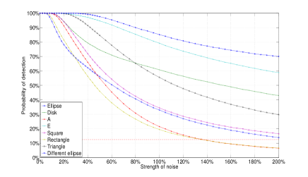
Figure 13: Stability of classification based on differences between ratios of singular values, when the fish is a straight ellipse. Here, $N_{\textrm{stabil}}=5.10^{4}$.

Figure 14: Classification with imaginary part of the PT, when the fish is a straight ellipse. All singular values are considered to discriminate between the targets. Here, $N_{\textrm{stabil}}=10^{5}$.

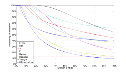
Figure 15: Classification with imaginary part of the PT, when the fish is a straight ellipse. Ratios of singular values are considered to discriminate between the targets. Here, $N_{\textrm{stabil}}=10^{5}$.