A twisted emission geometry in non-central Pb+Pb collisions measurable via azimuthally sensitive HBT

Abstract

We use the Ultrarelativistic Quantum Molecular Dynamics (UrQMD) model to simulate Pb+Pb collisions. In the freeze out geometry of non-central Pb+Pb collisions we observe a tilt of the particle emission zone in the collision plane away from the beam axis. We find that the magnitude of this tilt depends on the scale at which the distribution is measured. We quantify this “twisting” behavior with a parameterization and propose to measure it experimentally via azimuthally sensitive Hanbury-Brown Twiss correlations. Additionally we show that the twist is related to the emission of particles from different times during the evolution of the source. A systematic comparison between the theoretically observed twist in the freeze out position distribution and a mock experimental analysis of the model calculations via HBT correlations is shown.

1 Introduction

Quantum-Chromo-Dynamics (QCD) is the theory that describes the properties of strongly interacting matter. Currently only a few problems in QCD can be solved analytically. To explore the details of QCD experimentally one needs to compress and heat up QCD matter to regimes that were present microseconds after the Big Bang. Today similar conditions are present only in the interior of neutron stars or in heavy-ion collisions at relativistic energies. Several experimental programs at the SPS (e.g. NA49, CERES and NA50/NA60), RHIC (e.g. PHENIX, STAR, PHOBOS and BRAHMS) and at the LHC (e.g. ALICE, CMS and ATLAS) are dedicated to study the medium created in heavy-ion collisions. Due to the small scale and short lifetime of the reactions, only the momentum spectrum of the particles coming out of the interaction zone can be measured directly. However, the space-time structure of the collisions can be probed indirectly using Hanbury-Brown Twiss (HBT) interferometry. This technique uses two particle correlations to probe the space-time shape of the particle emission zone of relativistic heavy ion collisions. Extensive studies have been performed [1] to map out the dependence on transverse momentum ($p_{T}$), rapidity ($y$), collision energy ($\sqrt{s}$) and charged particle multiplicity. HBT interferometry measurements relative to the impact parameter direction yield additional insights about the shape and orientation of the emission region as a whole. Unfortunately only a small number of azimuthally sensitive HBT measurements have been reported so far [2, 3, 4]. However the beam energy scan initiative (RHIC-BES) at the Relativistic Heavy Ion Collider (RHIC) and the CBM-Experiment at FAIR will bring new measurements of this observable [5, 6] over a broad energy range.

In section 2 of this paper we explain how to extract the substructure of the tilt of the pion freeze out distribution in the event plane from the spatial freeze out distribution. We discuss a new feature of the source, the twist, not yet measured or discussed extensively in the literature. A parameterization of the twist and aspects of its physical origin are discussed. Section 3 suggests a phenomenological approach that allows to measure the twist experimentally and an example of the results from such an approach.

2 Analysis of the pion freeze out distribution

We use the well known Ultrarelativistic quantum Molecular Dynamics (UrQMD) approach to simulate the heavy-ion events for this paper. UrQMD is a hadronic non-equilibrium transport approach that produces particles via string fragmentation and resonance excitation and decay. For details of UrQMD the reader is referred to [7, 8, 9]. Previous HBT results of the model can be found in [10, 11, 12]

The anisotropic “almond” shape of the emission zone in the transverse plane created in non-central collisions is discussed extensively in the literature, as it leads to momentum-space anisotropies (elliptic flow) [18]. However, the spatial substructure of the emission region is much richer than its projection onto the transverse plane. The projection onto the reaction plane, $x-z$ (where $x$ is the direction of the impact parameter and $z$ is the beam direction)– even when selecting particles emitted only at midrapidity– is characterized by a nontrivial shape and anisotropies.

Transport calculations and three-dimensional hydrodynamic simulations generate distributions characterized by a tilt relative to the beam direction, which has been related to “antiflow” [13, 16] or a “$3^{\rm rd}$ component” of flow [19, 21]. In the transport calculations, the emission zone resembles to first order a tilted ellipsoid [16], an idealization which is shown in Fig. 1.

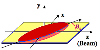
Figure 1: Orientation of the particle emitting zone (red) in the reaction plane and definition of the tilt angle $\theta_{S}$. Taken from [14]

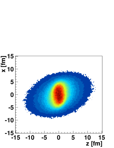
Figure 2: Projection of the pion freeze out distribution for Pb+Pb at $E_{lab}=8$ AGeV, $b=3.4-6.8$ fm, $|y|<0.5$ and $p_{\perp}<0.4$ GeV.

We parametrize the tilted freeze out distribution by a three dimensional Gaussian ellipsoid in space. In addition we allow that the ellipsoid is rotated by the angle $\theta_{S}$ (see Fig. 1) around the y-axis. This leads to Eq. 1 for the freeze out distribution $f$

$$f(x,y,z)\sim\exp{\left(-\frac{(x\cos{\theta_{S}}-z\sin{\theta_{S}})^{2}}{2\sigma_{x^{\prime}}^{2}}-\frac{y^{2}}{2\sigma_{y}^{2}}-\frac{(x\sin{\theta_{S}}+z\cos{\theta_{S}})^{2}}{2\sigma_{z^{\prime}}^{2}}\right)}.$$ (1)

In this equation x,y and z are the spatial coordinates, $\theta_{S}$ is the tilt angle and $\sigma_{x^{\prime}}$, $\sigma_{y}$ and $\sigma_{z^{\prime}}$ denote the Gaussian widths of the distribution where the primes on $\sigma_{x^{\prime}}$ and $\sigma_{z^{\prime}}$ signify that these correspond to the principal axes of the ellipse instead of the usual coordinate axes.

Analyzing the freeze out distribution in detail (see Fig. 2) reveals that the system is not characterized by one unique tilt angle, but exhibits a complex geometry. While the innermost part is almost aligned to the x-axis ($\theta_{S}\approx 90^{\circ}$) the tilt angle is significantly smaller at the outermost part of the distribution.

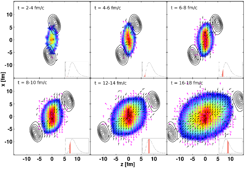
Figure 3: Shape of the freeze out region from pions frozen out at different times (colored surface). The contour lines depict the position of the spectators in each timestep. The vector field shows the direction of movement at each position and time. The black arrowheads contribute to the directed flow while the magenta arrows contribute to the antiflow. The inlay shows the freeze out luminosity of pions versus freeze out time. The shaded region in the inlay highlights the luminosity corresponding to the timestep in the overall picture.

The source of this structure is seen in Fig. 3. It shows the time evolution of the pion freeze out distribution (colored surface). The black contours represent the position of the spectators in each time step while the vector field depicts direction of the average velocity at each space-time point. The vector field is split into a directed flow (black arrowheads) and an antiflow (magenta arrows) component. To determine whether a given point in space-time is characterized by flow or antiflow, the average pion momentum $\overline{\vec{p}}$ is calculated for each (0.5-fm)³ cell in the $x-z$ plane. Cells with $\overline{p}_{x}\cdot\overline{p}_{z}>0$ (resp. $<0$) are considered to be dominated by flow (resp. antiflow).

From the time evolution it becomes clear that different angles in the tilt structure have their origin at different times of the evolution. In the beginning up to $t\approx 4$ fm/c only very few particles are emitted, without further reinteractions. After that more particles contribute to the freeze out. From $t\approx 4$ fm/c to $t\approx 10$ fm/c the emission pattern is dominated by the fact, that the spectator nucleons shadow the emission of particles in their direction. This gives rise to an antiflow [13] since most particles giving a positive contribution to flow are absorbed by the passing target and projectile nucleons. This automatically leads to a backwards tilt in the freeze out distribution from early times.

After $t\approx 10$ fm/c the spectators have moved on, so they no longer shadow the emission. At this point, about 1/3 of pion emission has occurred (see insets in Fig. 3). The momentum and spatial anisotropies evolve differently in the absence of the shadowing influence, leading to a time-dependent tilt angle. This pattern imprints itself onto the time-integrated freezeout distribution (Fig. 2) as a scale-dependent tilt angle– the twist. It is the time-integrated freezeout distribution that is experimentally accessible via HBT measurements, so any experimental sensitivity to the time evolution of the tilt is through this twist.

To underscore the importance of exploring this twist, we point out that even at the later stages of emission (final panels of Fig. 3), the antiflow component in the regions far from the retreating spectators is as strong as the flow component in the other regions. Thus, there are two components to antiflow in these collisions: shadowing effects in the early stage and preferential spatial expansion along the short axis of the distribution in the later stage. This latter component is the analog to the more familiar pressure-gradient-driven elliptic flow in the $x-y$ plane. The interplay between flow and the two sources of antiflow is complex, presumably energy-dependent, and may be crucial for understanding the details of $v_{1}$ measurements.

In most hydrodynamical modeling of elliptic flow, an anisotropic initial state is generated by some (often ad-hoc) mechanism, and then the system responds according to pressure gradients, equation of state, etc. In full transport calculations like UrQMD, there turns out to be at best an approximate factorization into two stages– the deposition of energy into the transverse plane at midrapidity, and the reaction of the system to the initial-state distribution. However, such a factorization is manifestly impossible when considering patterns in the $x-z$ plane, where the source is evolving violently even as it emits particles. Understanding $v_{1}$ and similar measurements requires a much more detailed understanding of the space-time evolution of anisotropic structures.

To explore this pattern quantitatively we fit different parts of the distribution separately, by defining equidistant (2 fm) rings in the x-z plane around the collision center. Then we perform separate fits for each section of the freeze out distribution taking into account only the part of the distribution between two adjacent rings. The y-direction is unrestricted for these fits. The results of this procedure are shown in Figs. 5 and 4. In Figure 4 the red contours are the pion freeze out distribution for Pb+Pb at $E_{lab}=8$ AGeV, $|y|<0.5$, $p_{\perp}^{\pi}<400$ MeV. The angle of the black line represents the result for $\theta_{S}(r)$ from the separated fitting, while its length describes the outer limit for the currently applied fit.

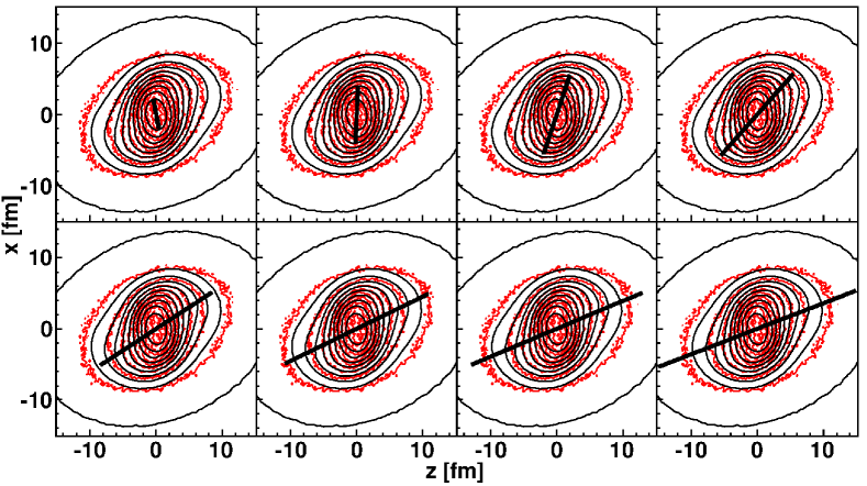
Figure 4: Fit to the pion freeze out distribution for Pb+Pb at $E_{lab}=8$ GeV, $b=3.4-6.8$ fm, $|y|<0.5$ and $p_{\perp}<0.4$ GeV. The red contour is the actual freeze out distribution from UrQMD. The black contour represent the three dimensional fit to the whole freeze out distribution. The black lines represent the fit results for the sphere shells. Their angle represents the fitted angle, while their length represents the radius of the fit sphere.

In Fig. 5 the results for the tilt angle of these fits are presented versus the radius of the fitted segment (red triangles).To characterize the source effectively we chose to parametrize the $\theta_{S}(r)$ dependence on $r$ by Eq. 2:

$$\theta_{S}(r)=\theta_{0}+\theta_{Mag}\exp{\left(-\frac{r^{2}}{2\sigma_{twist}^{2}}\right)}.$$ (2)

Inserting Eq. 2 into Eq. 1 we gain a new expression for the freeze out distribution, now with a radius dependent $\theta_{S}(r)$. The black contours Fig. 4 represent the projection of the three dimensional fit of the parametrized freeze out distribution to the actual freeze out distribution from UrQMD. It describes the overall shape reasonably well and provides a good description of the tilt angle. The black line in Fig. 5 shows the functional dependence of $\theta_{S}(r)$ extracted from Eq. 2 using the values for the parameters obtained from the full three dimensional fit.

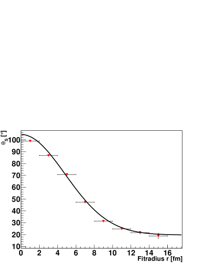
Figure 5: Radius dependence of the tilt angle for the fits with rings (red triangles) and for the full 3D-fit with a radius dependent $\theta_{S}(r)$ (black line). The system is Pb+Pb at $E_{lab}=8$ GeV, $b=3.4-6.8$ fm, $|y|<0.5$ and $p_{\perp}<400$ MeV.

3 Tilt and twist from azimuthally sensitive HBT calculation

The drawback of the procedure described in Section 2 is that it is not possible to measure the spatial freeze out distribution directly in experiment. If it were possible to measure the twist this would put additional constraints on many theoretical models. We propose to employ azimuthally sensitive HBT [2, 14, 15, 16] in a restricted momentum range to measure the tilt experimentally. Let us briefly outline the procedure to measure $\theta_{S}$ via HBT (independent of $r$).

As usual the correlation function is calculated using [17]

$$C(\bf{q},\bf{K})=1+\int d^{4}x\cos(q\cdot x)d(x,K)$$ (3)

where $C$ is the correlation function, $q$ is the four-momentum distance of the correlated particles, $K=(p_{1}+p_{2})/2$ is the pair momentum, $x$ is the particle separation four-vector and $d$ is the normalized pion freeze out separation distribution. For the azimuthally sensitive analysis of the HBT correlations the momentum space is subdivided in several azimuthal sections around the beam axis. For each of the sections an individual correlation function is computed. The azimuthal angle of the pair momentum vector determines in which correlation function each pion pair is counted.

Each of the correlation functions is then fitted separately with

$$C(\bf{q},\bf{K})=1+\lambda(\bf{K})\exp\left[-\sum_{i,j=o,s,l}q_{i}q_{j}R_{ij}^{2}(\bf{K})\right],$$ (4)

to obtain the HBT radii $R_{ij}$. For non-central collisions this leads to oscillating HBT radii with the azimuthal angle $\phi$. Doing a fourier decomposition it is possible to extract $\theta_{S}$ for low momentum pairs using

$$\theta_{S}=\frac{1}{2}\tan^{-1}\left(\frac{-4R_{sl,1}^{2}}{R_{l,0}^{2}-R_{s,0}^{2}+2R_{s,2}^{2}}\right),$$ (5)

where in $R_{\nu,\mu}$ the $\mu$ denotes the order of the fourier coefficient, e.g. $R_{s,2}$ is the second order fourier coefficient of the $R_{s}$ parameter. Details on this method and on finite bin width corrections can be found in [14, 17]. While Eq. 5 allows us to experimentally determine $\theta_{S}$ it does not give us any information on the $r$ dependence of $\theta_{S}(r)$ and it is not clear how to generalize the derivation of Eq. 5 to a $r$ dependent $\theta_{S}$. Thus we resorted to a phenomenological way to determine the twist.

It was already noticed in [14] that the twist in the freeze out distribution leads to a rising $\theta_{S}$ with the fit range of the correlation functions.This correlation can be attributed to the fact, that larger/smaller values of $q$ are sensitive to smaller/larger structures of coordinate space. To get a $\theta_{S}(r)$ we exploit this behaviour, by applying the same procedure described in Section 2 for the freeze out distribution in coordinate space, now to the correlation function in momentum space. Namely we generate correlation functions for eight $45^{\circ}$-wide bins in $\phi$ to do the azimuthal HBT analysis. We then define equidistant sphere surfaces in momentum space around the origin and do the azimuthal HBT analysis needed for $\theta_{S}$ in Equation 5 for each sphere shell between two adjacent sphere surfaces separately. As a result of this procedure we obtain a $\theta_{S}(q)$. The result for Pb+Pb, $E_{lab}=8$ AGeV, $b=3.4-6.8$ fm, $|y|<0.6$ and $p_{\perp}<0.4$ GeV is shown as red triangles in Fig. 6 versus $q_{fit}$, where $q_{fit}$ is the middle radius of each sphere shell.

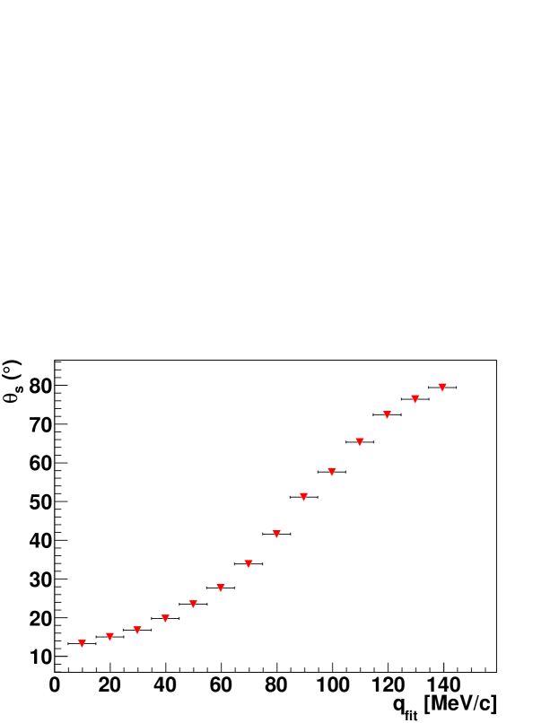
Figure 6: Results for $\theta_{S}(q)$ plotted versus $q_{fit}$, where $q_{fit}$ denotes the $q$ segment of the correlation function that is fitted. The investigated system is Pb+Pb at $E_{lab}=8$ GeV, $b=3.4-6.8$ fm, $|y|<0.5$ and $p_{\perp}<400$ MeV.

Indeed, Fig. 5 and Fig. 6 do bear a striking similarity if one keeps in mind, that larger $q$ values mean sensitivity to smaller regions of homogeneity and vice versa. In Fig. 7 we compare the results of both methods (see Figs. 5 and 6) in a single figure. The symbols show $\theta_{S}(q)$ versus 1/q (blue circles) and $\theta_{S}(r)$ versus r (red triangles). It is clear that a simple $r\sim 1/q$, as done for the plot reflects the relation between the spatial extension of the source and the region of homogeneity only qualitatively (there might be some other proportionality factor, that depends on the flow and temperature). Nevertheless it clearly indicates the momentum bin differential azimuthally sensitive HBT allows to capture the complicated source structure. Let us now compare the calculations to the expectations obtained from Eqs. 1 and 2. The dashed black line in Fig. 7 is a fit of equation 2 to $\theta_{S}(1/q)$. The description of the theoretical data points is very good and leads to $\theta_{Mag}$ and $\theta_{0}$ of both methods being similar to each other.

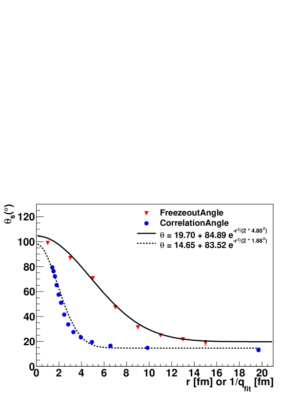
Figure 7: $\theta_{S}$ extracted via fits to the freeze out distribution (red triangles) and via fits to the HBT correlation functions (blue circles). The x-axis shows the fit radius $r$ for the freeze out distribution and the inverse of the momentum fit range $1/q_{fit}$ for the correlation functions. The dashed black line is a fit of equation 2 to $\theta_{S}$ from the correlation function. The full black line is also equation 2 but using the parameters of a fully three dimensional fit to the freeze out distribution with equation 1 using the $r$ dependent $\theta_{S}(r)$.

4 Summary and discussion

The analysis of the spatial pion freeze out distribution of a non-central lead lead collision from UrQMD features a scale-dependent tilt, or “twist”. The twist originates from antiflow and shadowing of pion emission at early times and the absence of shadowing at later times. To make the spatial twist experimentally accessible we have employed an azimuthally sensitive HBT analysis that allows to measure the tilt angle. Using the fact that pairs with small momentum difference are sensitive to large space-time structures and vice versa we calculated the tilt angle on different scales. The analysis shows that this procedure provides a qualitatively accurate picture of the radius dependence of the tilted freeze out distribution. This analysis enables us for the first time to use HBT correlations to disentangle the geometry of the source from different times up to a certain point. We conclude that the twist structure is in principle accessible by experimental HBT analysis and may allow to gain complementary insights into the early emission stages of the reaction.

References

References

- [1] M. A. Lisa, S. Pratt, R. Soltz and U. Wiedemann, Ann. Rev. Nucl. Part. Sci. 55, 357 (2005) [nucl-ex/0505014].
- [2] M. A. Lisa et al. [E895 Collaboration], Phys. Lett. B 496, 1 (2000) [nucl-ex/0007022].
- [3] J. Adams et al. [STAR Collaboration], Phys. Rev. Lett. 93, 012301 (2004) [nucl-ex/0312009].
- [4] D. Adamova et al. [CERES Collaboration], Phys. Rev. C 78, 064901 (2008) [arXiv:0805.2484 [nucl-ex]].
- [5] M. M. Aggarwal et al. [STAR Collaboration], arXiv:1007.2613 [nucl-ex].
- [6] C. Anson [STAR Collaboration], J. Phys. G G 38, 124148 (2011) [arXiv:1107.1527 [nucl-ex]].
- [7] M. Bleicher et al., J. Phys. G 25, 1859 (1999) [arXiv:hep-ph/9909407].
- [8] S. A. Bass et al., Prog. Part. Nucl. Phys. 41, 255 (1998) [Prog. Part. Nucl. Phys. 41, 225 (1998)] [arXiv:nucl-th/9803035].
- [9] Q. Li, M. Bleicher and H. Stoecker, Phys. Rev. C 73, 064908 (2006) [nucl-th/0602032].
- [10] Q. Li, M. Bleicher and H. Stocker, Phys. Lett. B 659, 525 (2008) [arXiv:0709.1409 [nucl-th]].
- [11] Q. -f. Li, J. Steinheimer, H. Petersen, M. Bleicher and H. Stocker, Phys. Lett. B 674, 111 (2009) [arXiv:0812.0375 [nucl-th]].
- [12] Q. Li, G. Graf and M. Bleicher, Phys. Rev. C 85, 034908 (2012) [arXiv:1203.4104 [nucl-th]].
- [13] J. Brachmann, S. Soff, A. Dumitru, H. Stoecker, J. A. Maruhn, W. Greiner, L. V. Bravina and D. H. Rischke, Phys. Rev. C 61, 024909 (2000) [nucl-th/9908010].
- [14] E. Mount, G. Graef, M. Mitrovski, M. Bleicher and M. A. Lisa, Phys. Rev. C 84, 014908 (2011) [arXiv:1012.5941 [nucl-th]].
- [15] M. A. Lisa, E. Frodermann, G. Graef, M. Mitrovski, E. Mount, H. Petersen and M. Bleicher, New J. Phys. 13, 065006 (2011) [arXiv:1104.5267 [nucl-th]].
- [16] M. A. Lisa, U. W. Heinz and U. A. Wiedemann, Phys. Lett. B 489, 287 (2000) [nucl-th/0003022].
- [17] U. A. Wiedemann and U. W. Heinz, Phys. Rept. 319, 145 (1999) [nucl-th/9901094].
- [18] J. -Y. Ollitrault, Phys. Rev. D 46, 229 (1992).
- [19] L. P. Csernai and D. Rohrich, Phys. Lett. B 458, 454 (1999) [nucl-th/9908034].
- [20] V. K. Magas, L. P. Csernai and D. D. Strottman, hep-ph/0101125.
- [21] L. P. Csernai, V. K. Magas, H. Stocker and D. D. Strottman, Phys. Rev. C 84, 024914 (2011) [arXiv:1101.3451 [nucl-th]].