The Micro-Arcsecond Scintillation-Induced Variability (MASIV) Survey III. Optical Identifications and New Redshifts

Abstract

Intraday variability (IDV) of the radio emission from active galactic nuclei is now known to be predominantly due to interstellar scintillation (ISS). The MASIV (The Micro-Arcsecond Scintillation-Induced Variability) survey of 443 flat spectrum sources revealed that the IDV is related to the radio flux density and redshift. A study of the physical properties of these sources has been severely handicapped by the absence of reliable redshift measurements for many of these objects. This paper presents 79 new redshifts and a critical evaluation of 233 redshifts obtained from the literature. We classify spectroscopic identifications based on emission line properties, finding that 78% of the sources have broad emission lines and are mainly FSRQs. About 16% are weak lined objects, chiefly BL Lacs, and the remaining 6% are narrow line objects. The gross properties (redshift, spectroscopic class) of the MASIV sample are similar to those of other blazar surveys. However, the extreme compactness implied by ISS favors FSRQs and BL Lacs in the MASIV sample as these are the most compact object classes. We confirm that the level of IDV depends on the 5 GHz flux density for all optical spectral types. We find that BL Lac objects tend to be more variable than broad line quasars. The level of ISS decreases substantially above a redshift of about two. The decrease is found to be generally consistent with ISS expected for beamed emission from a jet that is limited to a fixed maximum brightness temperature in the source rest frame.

1 INTRODUCTION

The discovery of centimeter wavelength, short term intra-day variability in some compact, flat-spectrum extragalactic radio sources (Heeschen, 1984; Heeschen et al., 1987) was of immediate and profound astrophysical consequence. This phenomenon, which was soon dubbed Intraday Variability (IDV; Wagner & Witzel, 1995), implied brightness temperatures up to $10^{21}$ K in extreme cases (Kedziora-Chudczer et al., 1997) if the variations were intrinsic. Such enormous brightness temperatures present a serious challenge to the current paradigm for the physics of extragalactic radio sources.

However, there is now overwhelming evidence that IDV results primarily from scintillation in the turbulent ionized interstellar medium of our Galaxy, commonly referred to as interstellar scintillation (ISS). This explanation was proposed by Heeschen & Rickett (1987) and has now been confirmed from several further lines of observational evidence. Time delays have been detected between the arrival times of the intensity fluctuations from ISS sources at two widely-spaced telescopes (Jauncey et al., 2000; Dennett-Thorpe & de Bruyn, 2002; Bignall et al., 2006). Further, annual cycles have been detected in the timescale of ISS sources (e.g. Jauncey & Macquart, 2001; Rickett et al., 2001; Bignall et al., 2003; Dennett-Thorpe & de Bruyn, 2003), a periodic modulation that most plausibly results from the change in relative velocity of the Earth and the scattering medium through the course of a year. Subsequently, a strong correlation has been found between the level of IDV and Galactic emission measure estimated from H$\alpha$ measurements (Lovell et al., 2008). This shows ISS to be the predominant cause of radio IDV. Though some questions remain (Jauncey et al., 2001; Krichbaum et al., 2002), interstellar scintillation is the only reasonable explanation of these observations (Jauncey et al., 2001).

Though an extrinsic (as opposed to intrinsic) origin for IDV points to less extreme physical conditions for the sources that exhibit this phenomenon, scintillators are still among the most extreme and active radio AGN known. For a source to scintillate, its angular size must be comparable to that of the first Fresnel zone (Narayan, 1992) which implies microarcsecond angular sizes for screen distances of tens to hundreds of parsecs. Such a high resolution cannot be achieved by any other existing technique, including space VLBI. Thus, interstellar scintillation has the potential to probe within a few light months of the central black hole (Bignall et al., 2003). Further, inferred brightness temperatures of a few scintillators are well in excess of $10^{14}$ K (Macquart et al., 2000) which implies Doppler factors of several hundred or more (Readhead, 1994) and is significantly higher than seen in VLBI surveys (e.g. Lister et al., 2009; Ojha et al., 2010). While Doppler factors very similar to those found in VLBI are implied from the ISS analysis of the Green Bank radio monitoring program of 146 compact radio sources (Rickett et al., 2006), an investigation of the properties of AGN that exhibit ISS is of considerable astrophysical interest, both because their extreme physical properties make them ideal probes of existing models of AGN physics and they probe phenomena at unprecedented resolution.

The Micro-Arcsecond Scintillation-Induced Variability (MASIV) survey was undertaken by Lovell et al. (2003, 2008) in order to construct a large sample of scintillating extragalactic sources. A key discovery from the MASIV survey is that both the number of sources showing ISS and their level of ISS variations appear to decrease with increasing redshift (Lovell et al., 2008). This result was obtained for the 275 (of 443) sources with measured redshifts. While 206 of these redshifts were obtained from the published literature, 69 of them were based on preliminary analysis of our unpublished optical observations. A primary goal of the present paper is to publish the full analysis of those optical observations and an additional 22 sources subsequently observed.

The apparent decrease in ISS with redshift is a new cosmologically important result. Its interpretation must include the cosmological prediction that the angular size of an object should initially decrease with redshift but start to increase above redshifts of about one. Observational evidence for this phenomenon has long been sought, but the best evidence to date is still only marginal (Gurvits et al., 1999). The MASIV sources were selected for their flat radio spectra and many are quasars. Thus any detailed interpretation must also address possible evolution in the beamed AGN jets presumably responsible for their very compact diameters. Alternatively, there could be scattering effects in the inter-galactic medium that could cause radiation from the more distant AGN to be scatter broadened so that their angular sizes are too great for them to scintillate in the interstellar medium of our Galaxy.

A follow-up to the MASIV Survey has been conducted in which the ISS of a subsample of 140 MASIV sources (70 with $z<$ 2 and another 70 with $z>$ 2) were observed simultaneously at 5 GHz and 8.4 GHz over a duration of 11 days using the VLA (Koay et al., 2011). These observations provided a means of determining the origin of the redshift dependence of ISS, by examining how the effect scales with frequency. This exploited the fact that intrinsic source size effects and scatter broadening both have different frequency dependences. The analyses and results were presented in Koay et al. (2012).

Our investigation of scintillators has been greatly handicapped by the lack of source redshifts. The MASIV survey found more scintillators among the weaker radio source sample, which also showed more extreme scintillation behaviour than their higher flux density counterparts. Since redshifts have been measured predominantly for the stronger radio sources, we particularly need to measure redshifts for the weaker sources. Redshifts are essential to determine physical properties including linear sizes, accurate brightness temperatures and luminosity distributions. Optical luminosities are also an important probe of the physics of Compton scattering. For high Lorentz factor jets, energy losses should be dominated by Compton scattering of the diffuse radiation field of the cosmic microwave background, starlight and reprocessed emission from the nucleus (Begelman et al., 1994). This energy will escape mainly at X-ray wavelengths but some is expected in the optical band. Thus redshifts are needed to calculate the luminosities in order to understand the total energy budgets of these extreme sources.

In this paper we present new redshifts obtained with the 2.56 m Nordic Optical Telescope (NOT) on La Palma and the 5 m Hale Telescope at Mount Palomar. We also present redshifts obtained from the literature whose reliability could be ascertained and optical magnitudes collated from the surveys and literature. Further, we look for relationships between the redshift, spectral classification, luminosity and the observed level of ISS variation and compare the results with a simple model for ISS.

Throughout this paper we adopt a cosmology with $\Omega_{m}=0.27,\Omega_{\Lambda}=0.73$ and $H_{0}=70$ km s^-1 Mpc^-1. We use the convention $S_{\nu}\propto\nu^{\alpha}$ for flux density at frequency $\nu$.

2 THE MASIV SAMPLE

The MASIV sample has its roots in two radio catalogues: CLASS (Cosmic Lens All Sky Survey; Myers et al. 2003) and JVAS (Jodrell Bank VLA Astrometric Survey; Patnaik et al., 1992; Browne et al., 1998; Wilkinson et al., 1998). Both of these were targeted surveys of flat-spectrum radio sources using the VLA at 8.4 GHz in the ‘A’ configuration. JVAS is effectively a bright sub-sample of the complete JVAS/CLASS sample, which consists of more than 11,000 sources with flux density down to 30 mJy (Myers et al., 2003). We note that the CLASS flux density limit is well below the 100 mJy flux density limit chosen for the MASIV sample (see below).

For MASIV observations, we wanted to target compact flat-spectrum sources that were unresolved at 8.4 GHz with the VLA and located north of the equator. As a first step, all CLASS sources with modeled source sizes $<$ 50 mas and all JVAS sources with $>$ 95% of their flux density in an unresolved component were selected. These selection criteria were chosen due to the way the data were presented in each catalogue: for JVAS, the peak and total VLA flux densities are listed; for CLASS the modeled component size is presented. Both criteria select those sources which are essentially unresolved point sources for short (0.5 - 1.5 minute) snapshot observations with the VLA in ‘A’ configuration (this is the highest resolution configuration of the VLA). Sources where the catalogues indicated the presence of any confusing sources – indeed, any emission outside of the unresolved target source – in the VLA field, were dropped from the sample, as selecting each MASIV target field to consist of a single, isolated point source greatly simplifies the analysis of variability. To obtain a flat-spectrum sample with spectral index $\alpha\geq-0.3$ ($S_{\nu}\propto\nu^{\alpha}$), these sources were cross-correlated with the NVSS catalogue (NRAO VLA Sky Survey; Condon et al., 1998), although we note that the observed flux densities in these catalogues were non-simultaneous.

The sample was next divided into strong and weak subsamples of about 300 sources each with the strong sample consisting of sources with $S_{8.4\,GHz}>0.6$ Jy and the weak sample consisting of sources with $0.103<S_{8.4\,GHz}<0.13$ Jy. Finally, the sources were selected to have uniform RA – $\delta$ distribution in order to have the best possible coverage for the VLA observations (for details see Lovell et al., 2003).

MASIV’s 5 GHz observations were carried out on this ‘core’ sample of 578 sources. Of these, 102 sources were removed in the analysis stage due to the presence of structure or confusion while one was removed due to an error in the initial sample selection process. This left a sample of 475 point sources common to all four epochs of MASIV observations. However, as described in Lovell et al. (2008), 32 of these sources were used as secondary calibrators in two or more epochs, which effectively removes their low-level (instrumental or real) variations in those epochs, relative to the other sources. These 32 sources were excluded from the final MASIV sample, leaving 443 sources for full analysis.

As the average flux densities of many sources from the originally defined radio “strong” and “weak” samples vary with respect to the original catalogued flux densities, we used the first epoch VLA data (Lovell et al., 2003) to set the dividing flux density to 0.3 Jy at 5 GHz. In the rest of the paper we refer to the radio strong sample of 229 sources (including the 32 secondary calibration sources for the optical analysis only, Section 4) and the radio weak sample of 246 sources.

Lovell et al. (2008) report which of these sources exhibited Intra Day Variability (IDV) and in how many epochs of observation were classified as variable. A structure function (SF) analysis of the flux density variations was also done, which provides a quantitative measure of the strength of the variation. The flux density was normalized by its mean and the average SF was computed from the 4 epochs and tabulated for each source as $D({\rm 2days})$, the SF at a time lag of two days. This quantifies the variations and was shown to be correlated with the interstellar electron column density, estimated from H$\alpha$ emission on that line of sight. The correlation confirms that the variations are indeed predominantly due to ISS. There are thus two ways of quantifying the ISS of a source, either as the number of epochs in which it was classified as variable or the 4-epoch mean $D({\rm 2days})$, where we note that no significance should be attached to values smaller than about $4\times 10^{-4}$ (for details, see Lovell et al., 2008).

3 REVIEW OF THE LITERATURE

The main goal of this work is to present the spectroscopic identifications and redshifts of the flat-spectrum, extragalactic radio sources that make up the MASIV sample.

3.1 Redshifts from the Literature

We searched for redshifts and spectroscopic identifications of MASIV objects in the literature starting from data repositories like the NASA Extragalactic Database (NED). Spectroscopic identifications and redshifts were found for the majority (171 of 229) of the radio strong sample sources. However, this is not the case with the weak sample (62 of 246). Most literature redshifts and spectroscopic identifications are from the 12th Véron-Cetty & Véron (2006) compilation of known AGN, hereafter VCV12. Identifications for 27 objects are from CGRaBS (Candidate Gamma-Ray Blazar Survey; Healey et al., 2008) and the rest from sources found using NED.

For those objects which had reported redshifts, we tried to locate their spectra and/or information about their emission lines (line identifications, equivalent widths) from which the redshift estimates were obtained. We classified the sources into categories A, B or C, based on the reliability of their redshift estimates. Sources with redshifts obtained from multiple reported emission lines or with spectra clearly showing multiple emission lines were placed in category A. If only a single line was reported with wide wavelength coverage, or the spectrum provided was of marginal quality, the source was placed in category B (see comments in Table 2). Redshift estimates of sources for which the spectra were not available, but where the process by which the redshifts were obtained were clearly described, were also placed in category B, as were three sources where imaging studies have detected the host galaxy but show featureless spectra. For these three objects, we adopted the imaging redshift which is estimated assuming the host galaxy is a “standard candle” (for details see Sbarufatti et al., 2005). Finally, objects in which the redshifts were indicated to be photometric, or where no further information could be found on how they were obtained, were placed in category C. Objects with (nearly) featureless spectra, with conflicting reported redshifts, or with redshifts estimated based on an intervening absorption system, were all placed in category C. Comments on archival redshifts that either were rejected or judged less reliable are in Appendix A.

3.2 Optical identification

In order to define the sample for optical spectroscopy and select appropriate observing resources, accurate optical identification was a prerequisite.

For optical identification we used the CDS client database to access three large area surveys, the Sloan Digital Sky Survey (SDSS), the Guide Star Catalog 2.3 (GSC) and the USNO-B1 Catalog. The SDSS DR5 (Adelman-McCarthy et al., 2007) is the primary catalogue for optical identification. It is complete down to $r$=22.5 ($\lambda_{eff}\sim$6230Å) with astrometric accuracy of about 0$\farcs$1 (Pier et al., 2003) and covers essentially the Galactic gap (RA $\sim$12^h $\delta\sim$30$\arcdeg$) and some smaller patches altogether about 8000 square degrees. As a secondary catalogue we used the GSC 2.3 (Lasker et al., 2008) which is compiled from scans of the POSS-II plates and has F magnitudes ($\lambda_{eff}\sim$6500Å) down to $\sim$20.5. This has poorer photometric (0.13-0.22 mag) and astrometric accuracy (0$\farcs$3-0$\farcs$4) than the SDSS. For 16 sources which were not found from the GSC2.3 we used USNO-B1 R2-magnitudes (Monet et al., 2003), which has poorer photometric accuracy than the GSC2.3 (Sesar et al., 2006). Of these sources ten are faint ($R2>$19.0), just visible from the POSS-I O-plates, and four are bright extended targets ($R2<$11.3). The ten faint objects might be missing from the GSC2.3 due to variability, while the four bright, extended objects may be missing due to the design of the GSC2.3. Finally, for eight faint sources we found optical magnitudes from the literature.

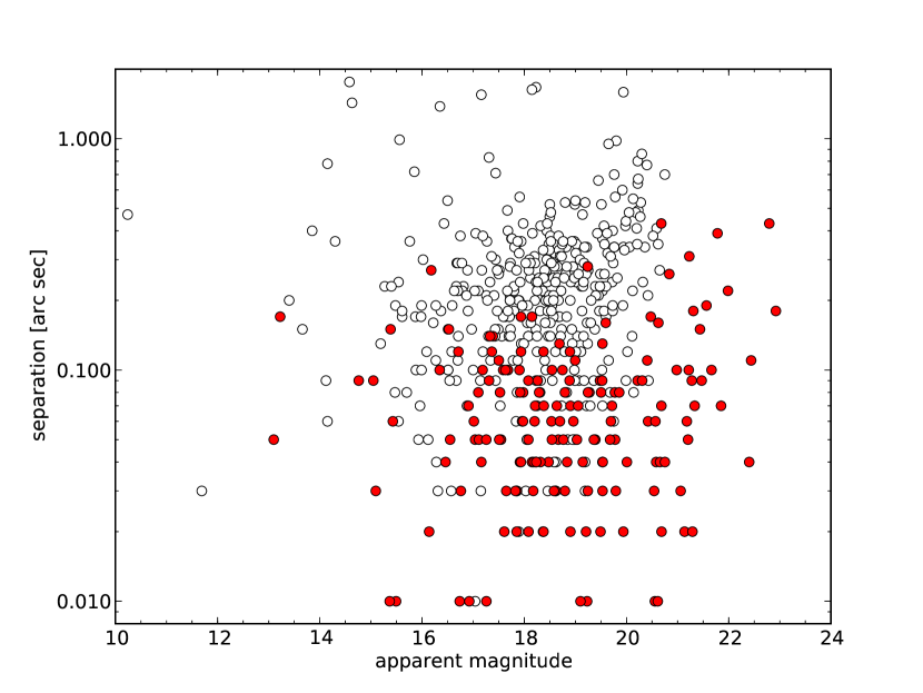
Figure 1: Apparent SDSS $r$-magnitude (red dots) and GSC2.3 F-magnitude (gray circles) versus separation between the radio and optical positions.

The initial search radius around the radio position was 5$\arcsec$. From SDSS DR5 we found 165 matches to a MASIV radio source within one arcsecond, with median $r$-magnitude of 18.7$\pm$1.8 (standard deviation of the distribution) and the faintest optical identifications having $r$=22.9. The mean separation increases from 0$\farcs$07 for $r<$ 20.5 mag sources to 0$\farcs$15 for the 37 sources with 20.5 $<$ $r$ $<$ 22.9. The GSC2.3 has 356 matches within 1$\farcs$5 with median magnitude of 18.4$\pm$1.5. The mean separation of $F<$ 19.5 sources is 0$\farcs$25 and for the 38 sources with $19.5<F<20.7$ it is 0$\farcs$39. Fewer than 10% of the GSC2.3 matched sources have separations greater than 0.5 arcsecond and only $\sim$2% have separations greater than one second of arc. In Figure 1 we show a plot of the measured separation versus apparent magnitude. In both the SDSS DR5 and GSC2.3 matched sources, the accuracy of the astrometry is as expected and decreases close to the limiting magnitude of the survey.

Multiple matches were found in 14 cases ($\sim$4% of the matches). Inspection of the data and visual inspection of the images (available from the CDS) revealed that close companions (8 sources), defined as those with a separation less than one arcsecond, were from separate epochs. This suggests that there is only a single source, but the astrometric solution is slightly different from epoch to epoch. For the remaining six sources the nearer object was selected as the optical counterpart and a second target was found with the angular distance 2.5-4.9 arcseconds from the radio source. Of the 356 GSC2.3 detected objects, 133 also have SDSS DR5 magnitudes, hence we are left with 223 sources with only F-magnitudes. Down to a Galactic latitude of 5 degrees, all SDSS and GSC2.3 matches had only a single source within the search radius. Table 1 summarizes the SDSS and GSC identifications.

In addition we defined a subsample, ($08^{h}<$RA$<16^{h}$ and $\delta<64^{\circ}$), which covers roughly the SDSS DR5 sky area (hereafter ‘SDSS sample’). Of the 79 radio strong sources, all but one secondary calibrator source have optical identifications. Optical identifications are available for 82 out of 95 sources in the radio weak sample.

3.2.1 Combining GSC2.3 and SDSS DR5 Data

We transformed the GSC2.3 and SDSS DR5 data to the common magnitude system using

$$R_{SDSS}=r-0.272(r-i)-0.159$$ (1)

by Chonis & Gaskell (2008) for the SDSS data. This is derived using SDSS DR5 and Landolt (1992) data for $r>$ 14 magnitude stars. For the $r<$ 14 stars they found a systematic magnitude difference, however we have only two such bright targets.

We obtained the GSC2.3 F- and N-magnitudes for the standard stars, which were observed more than four times by Landolt (2009) where we found (almost) a one to one correspondence

$$R_{GSC}=F.$$ (2)

The $F-N$ color term and zero point corrections are small and are omitted (see Appendix B for details). The USNO-B1 R2-magnitudes were converted in a similar way as the $F$ magnitudes. For 249 sources with 13 $<F<$ 19 the average magnitude difference $F-R2$ is $\sim$-0.07. Taking into account the small number of $R2$-magnitudes and the magnitude offset, the possible bias to the global properties is negligible.

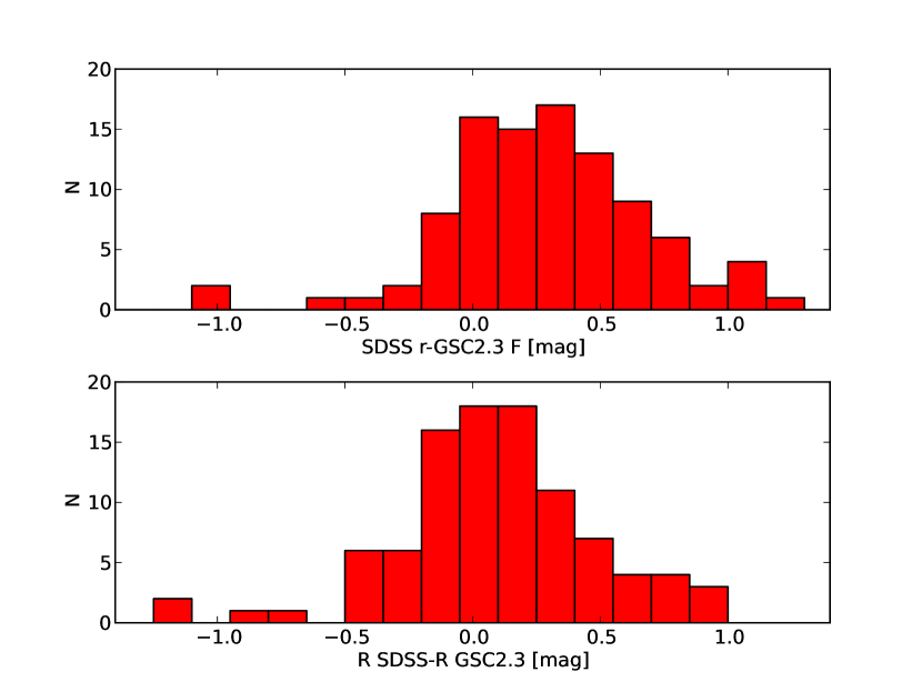
Figure 2: The histogram of the magnitude difference for objects with both SDSS and GSC identification. The bottom panel shows the converted R-magnitude difference.

We checked the common magnitude system by selecting all targets with SDSS photometry and GSC2.3 $F$ magnitude between 16.5 and 19.5, altogether 97 sources. The median $r$ - $F$ magnitude difference is 0.3$\pm$0.4 and after the $R_{SDSS}-R_{GSC}$ transformations the median difference is 0.1$\pm$0.4 (Figure 2) suggesting that the systematic difference between the transformed $R_{SDSS}$ and $R_{GSC}$ magnitudes is small in comparison to the uncontrollables, such as variability of the sources and photographic plate sensitivity changes.

The magnitudes are integrated magnitudes and there has been no attempt to separate the host galaxy contribution from the nucleus or correct the emission line fluxes. For optically extended sources (all low redshift, $z\lesssim 0.2$ sources as well as Sy2/NLRG-type objects at higher redshift) the absolute magnitude includes both the core and the host galaxy. For example, J0057+3021 (NGC 315) has USNO R magnitude $\sim$11.1 however the core R-magnitude is $\sim$19.8 (assuming V–R=0.3; Verdoes Kleijn et al., 2002). Also, the GSC2.3 photometry pipeline was tuned for point sources, thus there is a systematic overestimate for bright non-stellar magnitudes (Lasker et al., 2008).

All the magnitudes were de-reddened using the $E(B-V)$ values and the relative extinction values from Schlegel et al. (1998). In Table 2 and for the optical luminosities, we refer to $R_{SDSS}$ and $R_{GSC}$ as $R$-magnitude.

3.2.2 Radio and Optical Properties

The optical identification rate, combining the results from the SDSS DR5 and GSC2.3 catalogues, is $\sim$ 86% for the radio strong and $\sim$ 77% for the radio weak sample. However, since the two catalogues have different sky coverage and hence different Galactic latitude coverage, this could bias the identification rate. Therefore, using only the (all sky) GSC2.3 catalogue, the strong sample has $\sim$ 80% (187) of F-magnitudes brighter than 20 compared to $\sim$ 60% (146) for the weak sample.

Including empty fields, the median optical flux density of the strong radio sample is $\sim$0.15 mJy (18.2 mag) decreasing by a factor of 3.2 to $\sim$0.047 mJy (19.5 mag) for the weak sample. In comparison, the median radio flux density decreases by a factor of 7.4, from $\sim$0.89 Jy to $\sim$0.12 Jy in the two samples. If we were to use this radio flux ratio to calculate the weak radio sample median optical magnitude from the strong radio sample mean optical magnitude, it would yield a $R$-magnitude of 20.1 for the weak sample. The $k$-correction difference between the weak and strong samples is unknown, but most likely it is $\sim$0.2 magnitudes or less on average (e.g. Wisotzki, 2000), assuming the average redshifts of 1.2 and 1.8 for the strong and weak samples respectively (see below).

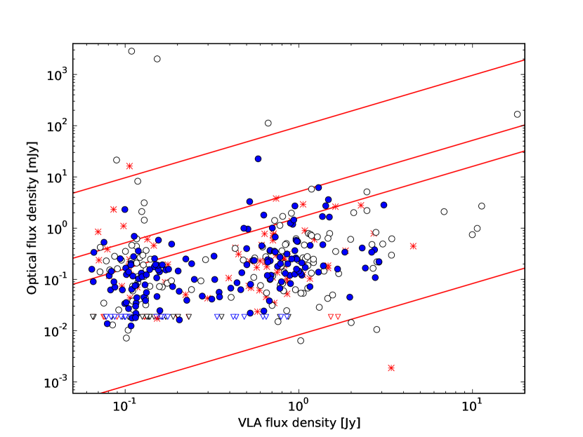
Figure 3: 5 GHz flux density vs optical flux. The blue circles, red stars and open circles are for variable, non-variable and intermittently variable, respectively. The magnitude upper limits (R=20.5) are indicated with blue, red, black triangles for variable, non-variable and intermittently variable, respectively. The diagonal lines indicate constant radio–optical spectral index -0.2, -0.45, -0.55 and -1.0 from top to bottom.

Figure 3 shows the optical versus radio flux density with diagonal lines indicating constant radio-optical spectral index (defined by $S_{\nu}\propto\nu^{\alpha_{ro}}$), which has only been corrected for Galactic extinction and lacks any $k$-correction because 40% of the radio weak sample objects have unknown redshift. The top line corresponds to $\alpha_{ro}$=$-$0.2, the generally accepted radio quietness limit (Stocke et al., 1985). Although there appears to be no detailed correlation between optical and radio flux density, the weak sample is on average one optical magnitude fainter than the strong sample. The radio weak sample also appears to have an even larger spread than does the radio strong sample. The weak sample has 17 sources with $\alpha_{ro}>-0.45$ and the strong one only five. Close to $\alpha_{ro}$=-1.0 both samples have many optically empty fields thus we cannot draw any conclusions about the underlying distribution. It is also important to note that the non-simultaneous nature of these radio and optical observations will further increase the scatter. The difference between the radio to optical flux ratios of the radio strong and weak samples is statistically significant. Running the ASURV Kaplan-Meier estimator (Avni et al., 1980), the probability that the two samples are drawn from the same parent population is small ($P<$0.01%). This holds for the ‘SDSS sample’ and also for the whole sample using a shallower GSC2.3 limiting magnitude.

Our results indicate that the radio faint objects are optically “brighter” than expected using the radio strong objects as reference. The explanation for the difference is not clear. One possibility is that the radio weak sources have larger host galaxy contributions in optical than radio strong objects. Another possibility is that the average spectral energy distributions of the strong and weak sources are different, perhaps due to differing contributions of the accretion disk (“big blue bump”) to the optical flux density or different amounts of dust.

4 SPECTROSCOPIC FOLLOW-UP

The new redshifts reported in this paper were obtained using the 2.56 m Nordic Optical Telescope (NOT) which is located at Roque de los Muchachos, La Palma, Canary Islands, Spain and the 5 m Hale Telescope at Mount Palomar, California, USA. Most of the NOT data were obtained during two observing runs (July 3rd to 7th, 2005 and July 22nd to 28th, 2006) supplemented by a few additional nights between January 2004 and July 2007. The Mount Palomar data were obtained during an observing run from August 9th to 10th, 2007. Most fields were pre-imaged at NOT with deeper and better image quality than the SDSS frames to verify the optical identification of the radio source. Altogether 90 objects were observed at NOT and 28 objects were observed at Palomar with some targets observed at both telescopes.

At NOT, low resolution spectra were obtained using the Andalucia Faint Object Spectrograph and Camera (ALFOSC) with Grism 4 (300 rulings/mm, 3200–9100 Å, dispersion of 3Å/pixel) with second order blocking filter giving wavelength coverage about 3800–9100 Å. However, in practice the NOT red limit of the spectrum is reduced to about 8000 Å  due to strong fringing. We used Grism 6 (600 rulings/mm, 3200–5550 Å) or Grism 3 (400 rulings/mm, 3200–6700 Å) for objects with a single detected line at about 5000 Å   in order to confirm the redshifts from either MgII, CIII] or the Ly-alpha line. The NOT run in 2005 was photometric, based on Carlsberg Meridian Telescope (CMT) data, with seeing of 0$\farcs$6-1$\farcs$4 and the 2006 run had some dusty and/or non-photometric nights with 0$\farcs$7-1$\farcs$1 seeing. At Hale, the Double Spectrograph (DBSP) was used with a setup of 600 lines on the blue arm (3400–5400Å, $\sim$1Å  per pixel) and 158 lines for the red (5400–9500Å, $\sim$4.9Å  per pixel) with either 1$\farcs$0 or 1$\farcs$5 slit giving continuous wavelength coverage from about 3400 to 9500 Å.

Most of the targets were observed with the slit in parallactic angle in order to reduce the light losses in blue. We note that, each spectroscopic target has a characteristic AGN spectrum and there is no evidence of any spurious counterparts. In two cases the nearby companion was put on the slit and in both cases the object closer to the radio source had a characteristic AGN spectrum while the companion had a typical stellar spectrum. For the NOT data, an internal flat field (Halogen) image was obtained before each science exposure, in order to improve the fringe correction at the red end. In addition, several HeNe images were taken during the night for the wavelength calibration. The DBSP calibration frames, dome flats, HeNeAr (red arm), FeAr (blue arm) images, were taken morning and evening. The data were reduced using standard IRAF procedures including bias subtraction, flat field correction using internal flat field lamp and wavelength calibration. Before extracting the spectrum, cosmic rays were removed from individual spectrograms. The majority of the spectroscopy targets have R-magnitude between 17 and 21, with a median of 18.8.

The redshifts were determined from the narrow emission lines (e.g. [O III]$\lambda\lambda$ 4959, 5007, [O II]$\lambda$ 3727) whenever possible, or from strong broad emission lines otherwise, typically H $\beta$, MgII , C III], C IV or Ly$\alpha$. The new redshifts are based on two or more line identifications. However, in four cases with wide spectral coverage and high S/N, we assumed the line to be MgII , as if the line were to be C III], we would have expected to detect C IV] or MgII . In Table 2 we list, respectively, source name, RA, declination, first epoch 5 GHz flux density, epochs of variability (at 5 GHz), $D({\rm 2days})$, Galactic reddening, de-reddened R-magnitude, R-magnitude reference, redshift, spectroscopic identification with the original references and a comment. Selected objects are discussed in Appendix A and C. Objects with only a single detected emission line are listed in Table 3.

4.1 Classification Scheme

On the basis of the optical spectrum the sources have been divided into three main groups: Type 0 objects with weak emission lines (mainly BL Lacs), Type 1 objects with strong and broad emission lines (mainly FSRQ) and Type 2 objects with strong and narrow emission lines (mainly Seyfert 2’s). In the context of AGN unification schemes, Type 0 and Type 1 objects have their Doppler boosted relativistic jet aligned close to the line of sight with Type 2 objects seen at a larger angle in such a way that the broad line region is obscured by a dusty torus (see review by Urry & Padovani, 1995). The spectroscopic classification scheme is adapted from previous works e.g. Laurent-Muehleisen et al. (1998), Caccianiga et al. (2002b) and Caccianiga et al. (2008). Many observed properties of the AGN, such as emission line equivalent widths ($EW$) and luminosities have continuous distributions. Hence the division between, for instance, Type 0 and Type 1 based on equivalent widths $EW$ or between Seyfert 1 and FSRQ based on optical luminosity depend on the dividing line chosen. The VCV12 classifies all objects fainter than $M_{B}=-23$ (using VCV12 cosmology and magnitudes) as (low luminosity) AGN, which is converted to our cosmology and R-band resulting in a QSO vs radiogalaxy (RG) limit $M_{R}=-22.8$. As noted by the VCV12, the $M_{B}=$–23 is an arbitrary limit without any physical reason. Due to different source classification schemes, and/or to variability, a QSO might have been classified as an AGN in one epoch but as an FSRQ at another epoch, and vice versa. For example, a strong radio source, J 1506$+$3730 is classified as an AGN by Healey et al. (2008), NLRG by Sowards-Emmerd et al. (2004) and Sy2 by VCV12. Also, in some cases the classification depends on S/N, e.g. a weak AGN-core with dilution by the host galaxy where broad emission lines might be undetected; for J 0057$+$3021, Ho et al. (1995) reported a broad $H_{\alpha}$ line, but a later study could not confirm it (Gonçalves & Serote Roos, 2004).

We describe our classification scheme below. Note that all the line equivalent widths (EW) are rest frame values:

0a) BL Lacs: objects with no lines or line rest frame $EW<$ 5Å  and $C<25\%$, where contrast C is defined as

$$C=(f_{+}-f_{-})/f_{+},$$ (3)

where $f_{-}$ is the mean flux in the 3750–3950 Å  range and $f_{+}$ in the 4050–4250Å  range where flux is measured in frequency. In the case of moderate S/N we give only tentative spectroscopic identification.
0b) BL Lac candidates: $25<C<40\%$ and strongest line $EW<40$ Å.
0c) Passive elliptical galaxies (PEG): $C>40\%$ and $EW<40$Å.
1a) Flat spectrum radio quasar (FSRQ): at least one permitted line excluding $H\alpha$, line FWHM $>$ 1000 km/s and $M_{R}<$ -22.8.
1b) Seyfert type 1 galaxies: $M_{R}>$ -22.8, the subclass has been defined based on the $H\beta$/[O III]$\lambda$5007 line ratio (Winkler, 1992).
1c) Narrowline Seyfert1/QSO (NLSy1/NLQSO): At low redshift: $H\beta$/[O III]$\lambda$5007 $<$ 3 and $H\beta$ $<$ 2000 km/s. For the $z>1.5$ targets: rest frame line width 1000-2000 km/s and the relative strength of the He II emission line compared to C IV following Heckman et al. (1995); Caccianiga et al. (2008). Type 1 objects have weak He II emission line.
2a) Narrow line Radio galaxy (NLRG): line FWHM $<$ 1000 km/s and $M_{R}<$ -22.8.
2b) Seyfert type 2 galaxies: $M_{R}>$ -22.8, the subclass has been defined based on the $H\beta$/[O III]$\lambda$5007 line ratio (Winkler, 1992).
2c) Galaxy: $C>40\%$, absorption lines e.g. Mg I and no emission lines

Low redshift sources are the most problematic to classify as host galaxy dilution can hide broad lines and can reduce the line EW. Also the non-thermal continuum can be difficult to detect. Fortunately only four of our follow-up targets are at low redshift ($z<$ 0.2), suggesting that the bias from the uncertain spectroscopic identification is small.

4.2 Summary of the spectroscopic follow-up

We report 79 new redshifts with spectroscopic identifications, 7 new BL Lacs with featureless spectra, and twelve objects with a single emission line of which six have a tentative redshift (Table 3 and Appendix C). We confirm the BL Lac status of nine objects, and confirm the archival redshifts as well as spectroscopic identifications for nine other objects. We also re-classify two BL Lac objects using our own data (Appendix A). Spectroscopic identifications from the literature were reviewed using the same scheme as for our own data, whenever possible. In some cases this led us to adopt a different classification than NED (see appendix A). Example spectra of our own observations are shown in Figure 4.

4.3 RESULTS AND SAMPLE PROPERTIES

Here we present 347 MASIV sources which have their spectra classified, either from the literature or based on our own data (Table 2). The radio strong sample is 91% (208/229) complete and the radio weak sample is 57% complete (139/246). Of the twenty-one radio strong sources without spectroscopic identification, seven have magnitudes from the surveys or literature, with R-magnitude between 17.3 and 23.99.

In Table 4 we summarize the number of sources in each optical spectral classification, separating the radio strong and weak subsamples. It shows that Type 1 sources are the most common, comprising 78% of both the radio strong and weak samples. About 18% of the radio strong sources and 16% of the radio weak sources have Type 0 spectra. A small minority of the sources have Type 2 spectra, 4% and 6% of the radio strong and radio weak samples, respectively. It also shows that almost all Type 1 sources are optically luminous FSRQs. In Table 5 we compare the identifications based on the present sample and the ‘SDSS sample’. The results suggest that the two samples have similar distributions of the sources for both radio strong and weak subsamples. Also the redshift distributions are identical. This suggests that the observed sample is representative in comparison to the full 475 object sample.

Though broadly similar, there is some difference in the spectroscopic identifications of the radio strong and weak samples. The radio weak sample appears to have slightly more low luminosity AGN (e.g. PEG, LINER, HII-region, Galaxy) and fewer BL Lac objects than the radio strong sample. An increasing number of low luminosity objects are expected to be detected as the flux limit of the sample decreases. At low redshift ($z<0.2$) most (7 out of 8) of the radio strong sample objects are BL Lacs or have broad emission lines, in contrast to the weak sample, where half (6 out of 12) of the $z<0.2$ objects have narrow emission lines or “galaxy” type spectra and a further five are classified as PEG. Also, the PEG and galaxy type objects are absent in the radio strong sample.

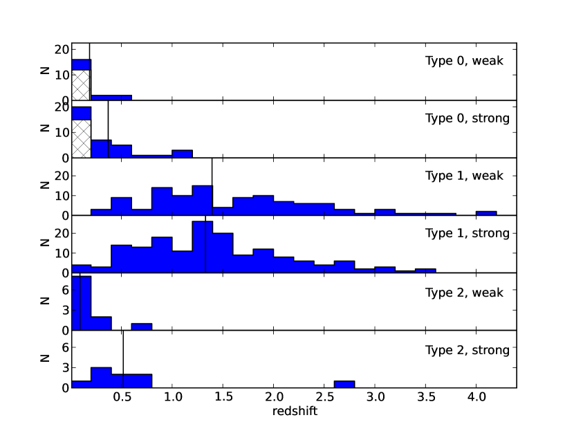
Figure 5: Redshift histograms of MASIV subsamples selected by 5 GHz flux density and optical spectral type. The BL Lacs with featureless spectrum are in the first bin of Type 0 panels. The vertical line in each subplot indicates the median redshift.

All together, redshift information is available for 319 sources. Figure 5 shows the redshift distributions of subsamples divided by the optical spectral classification and the MASIV first epoch 5 GHz flux density. For Type 1 sources the median redshift increases from 1.3 to 1.4 as the median (5 GHz) flux density decreases from 0.86 to 0.12 Jy. The Type 1 radio strong sample has a clear maximum in the distribution, but the radio weak sample has a fairly flat distribution between 0.7 and 2.0. Of the Type 1 sources $\sim$20% of the radio strong and $\sim$29% for the radio weak sample have $z>$ 2.0. The redshift trend due to the flux density limit is similar to that seen from the previous blazar surveys e.g. from S5 $z_{mean}$= 1.18 (limit 1 Jy) to S4 $z_{mean}$= 1.3 (limit 0.5 Jy) to DXRBS $z_{mean}$=1.56 (limit 0.05 Jy) (Landt et al., 2001). Most of the Type 0 or Type 2 sources have measured redshifts of less than one and almost 50% of the Type 0 sources are without a redshift.

We note that there might be a small number of mis-classified objects. As in every survey, the signal to noise ratio of the spectroscopic data is not always optimized for spectroscopic classification but for measuring the redshift. However, in most cases there is no ambiguity in our source classification. As our main results and conclusions are based on Type 1 sources (see below), the effect of some mis-classified objects is not significant.

4.4 MASIV and other Blazar Surveys

In Table 6 we compare spectroscopic identifications, limiting magnitudes and the radio flux density limit of MASIV with some other blazar surveys. The DXRBS sample (Padovani et al., 2007), is selected by cross-correlating X-ray sources with radio sources ($S_{5GHz}\gtrsim$ 50mJy). The CGRaBS (Healey et al., 2008) has flat spectrum radio sources selected from the CRATES (Healey et al., 2007) survey with $S_{4.8GHz}>$ 65 mJy, where the aim is to provide a catalogue of likely $\gamma$-ray loud AGN. This selection is based on a figure of merit (FoM) which measures the likelihood that an individual radio/X-ray source is associated with a known $\gamma$-ray source. In terms of selection criteria the CLASS blazar survey (CBS) (Marchã et al., 2001; Caccianiga et al., 2002b) is most similar to MASIV. The CBS has flat radio spectrum sources with the weakest sources $S_{5GHz}\gtrsim$ 30mJy and red magnitude $\leq$ 17.5. It is interesting to ask how the source identification differs between the MASIV selection criteria in comparison to the previous blazar surveys.

The DXRBS classification into the categories of “Radio Loud Quasar, BL Lac and Radio Galaxies” is almost identical to our Type 1, Type 0 Type 2. The possible difference is that they might classify “PEG” as “Radio Galaxy” and their survey is nearly complete ($\sim$95%, Padovani et al., 2007). The CGRaBS classifies objects as FSRQ (Type 1), AGN (Type 1), BLL(Type 0), NLRG(Type 2) and GALAXY (Type 2) where our corresponding classifications are in parenthesis. CGRaBS is about 79% complete with respect to the entire survey and 85% for objects with known R-mag$<$ 23. The comparison between the CBS ($\sim$91% complete; Caccianiga & Marchã, 2004) and MASIV is straightforward, as the MASIV classification is adopted from the CBS.

The distribution of the spectroscopic classes is almost identical between MASIV and the DXRBS and the CGRaBS with slightly more broad line quasars in MASIV than other surveys. The main difference between the CBS and MASIV is that the CBS has more low redshift Type 2 objects than MASIV. This difference remains when using similar radio (‘CBS rb’) and optical flux density (‘MASIV ob’) limits for these samples. This indicates that the selection of compact radio structure in defining the MASIV sample, filters out nearby Type 2 objects and favors FSRQs. Probably as a result of its bright optical flux density limit, the CBS has at least 40% of low redshift ($z<$0.15) sources. In contrast, MASIV has 4% for the total sample, 1% and 6% for the radio strong and weak samples, respectively. In all these cases it is assumed that the BL Lacs without redshift have $z>$0.15. Another difference between MASIV and the CBS is that sources that are optically less luminous but powerful in the radio (Figure 6 top panel, where $M_{R}>-23$ and $P>10^{26}$ W/Hz) are missing from the optically bright CBS sample.

The source and the redshift distributions of the MASIV, DXRBS and CGRaBS samples are similar. There might be slightly fewer $z>$ 3 sources in CGRaBS ($\sim$ 3%) than in MASIV ($\sim$5%). The difference could be, for example, due to incompleteness of the MASIV sample or pre-selection of only compact radio sources for the MASIV sample. MASIV has fewer low radio power FSRQ sources ($P_{r}<$ 10^25.5 W/Hz) than DXRBS ($22\%$; Landt et al., 2001), but about the same amount ($\sim$2-3%) as the combined 1-Jy and S4 samples. Some of the sources classified as “galaxy” might have weak broad lines which are not detected due to dilution by the host galaxy continuum and/or insufficiently high signal-to-noise ratio of the data.

Apart from decreasing the number of low radio power sources, using compact radio core selection increases the number of objects in the MASIV sample that have featureless optical spectrum i.e. are classified as BL Lacs. Specifically, it is interesting to note that IDV4 (i.e. IDV detected in all four MASIV epochs) is one of the most effective preselections to find BL Lac objects. The use of persistent IDV as a selection criterion strongly favours BL Lac objects with 43% of the MASIV sources showing IDV in all four epochs identified as BL Lac objects. In comparison, a radio–X-ray selection in the XB-REX sample (Caccianiga et al., 2002a) and DXRBS (Padovani et al., 2007) have a BL Lac fraction of 25% and 18% respectively. However, $\gamma$-ray loudness may be an even stronger selector of BL Lacs with about 50% of Fermi/LAT identifications being BL Lacs (Abdo et al., 2009).

Lister et al. (2001) studied the IDV properties of the Pearson-Readhead compact extragalactic radio sources and found that IDV sources have smaller emission line widths and lower 5 GHz luminosites than non-IDV sources. Their results about line widths are consistent with our findings that 25 to 40% (for IDV1 through IDV4 subsamples) of the MASIV IDV sources are BL Lac objects and that 70% of the BL Lacs are IDV sources. Whether there is a correlation between IDV and line width amongst the Type 1 sources will be studied in a future paper. The 5 GHz luminosity difference found by Lister et al. could be due to combining FSRQs and BL Lacs into one IDV/non-IDV sample, and the different redshift distributions of the IDV and non-IDV samples.

5 Discussion

5.1 Dependence of ISS on 5 GHz flux density and optical spectral type

The correlation between IDV and the 5 GHz flux density was discovered in the MASIV survey (Lovell et al., 2003) and later confirmed by Lovell et al. (2008). In the latter work, the variability of the flux density was studied using two complementary methods (see Section 2): $D({\rm 2days})$ which combines all the data in a statistical estimator; and a visual analysis of each light-curve at each epoch, which classified each source at each epoch as variable or not variable and so allowed an estimation of the duty cycle in the variability. Sources were classified as “ISS” if they were found to be variable in 2 or more epochs and as “non-ISS” otherwise.

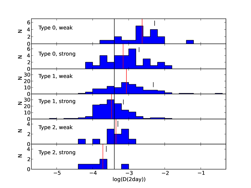
Figure 7: $D({\rm 2days})$ histograms of MASIV subsamples selected by 5 GHz flux density and optical spectral type. The black vertical line at $-3.4$ indicates the limit where SF-analysis suggests variability. In each subplot the red vertical line indicates the median value and the black line the mean value.

To study the flux density/ISS correlation in detail, we divided the sample by the flux density and spectroscopic type. Figure 7 shows the $D({\rm 2days})$ histograms of the MASIV subsamples. There is a clear increase of the median and mean $D({\rm 2days})$ as the flux density decreases and this is seen in all spectral types separately. One can see that many of the distributions in Figure 7 are significantly skewed, having a tail extending to high values. When binned on a linear scale the distributions are more strongly skewed. A measure of this skewness is that the mean values of $D({\rm 2days})$ are considerably larger than the median, since the rare high values influence the mean but have little effect on the median.

The Kruskal-Wallis (KW) test indicates a $\sim$0.4% probability that the radio strong and radio weak Type 0 samples have equal median $D({\rm 2days})$. The probability that Type 1 radio strong and weak samples have similar median is negligible ($p_{KW}<0.01\%$). Similarly, the Kolmogorov-Smirnov (KS) test indicates that the Type 0 radio strong and weak distributions of $D({\rm 2days})$ are drawn from the same parent population with a probability of 0.1%; for Type 1 sources this becomes $p_{KS}<$ 0.01%. For Type 2 objects the KW and KS tests indicate the same median or parent population with less than 5% probability, however the full sample contains only 19 objects and their $D({\rm 2days})$ values are typically at or below the threshold (0.0004) for significant variation. This indicates that the $D({\rm 2days})$ has a $S_{5GHz}$ dependence and this holds for Type 0 and Type 1 sources with high statistical confidence. A similar, but less significant, trend is also seen for Type 2 sources. We note that we have similar results when comparing the 5 GHz flux density distributions for sources drawn from the ‘SDSS sample’. Thus we confirm the IDV–$S_{5GHz}$ flux density dependence found earlier and show that this correlation is present at least for Type 0 and Type 1 sources.

In previous studies of IDV, the optical spectroscopic type of the objects has not been considered. Figure 7 and Table 7 suggest that the IDV properties depend not only on the 5 GHz flux density, but also on the optical spectral type. Although the statistical tests indicate a clear difference between the distribution of $D({\rm 2days})$ in the Type 0 and Type 1 sources for the full sample, there are interdependencies that could cause an apparent correlation.

To study the apparent correlation between spectral type and ISS, we first ask if the different redshift distributions of Type 0 and Type 1 sources could cause the difference in the $D({\rm 2days})$. From previous studies, BL Lacs and FSRQs have been found to have different observed redshift distributions (e.g. Giommi et al., 2012) with BL Lacs having a lower median redshift than FSRQs. As many (25 out of 59) of our Type 0 sources are without known redshifts, it is probable that the redshift distributions of the Type 0 and Type 1 sources are different. Hence it is difficult to compare Type 0 and Type 1 sources accurately.

First we compared the $D({\rm 2days})$ distributions of Type 0 sources with known redshift ($z_{max}\sim$ 1.15, N=16) to Type 1 sources with $z<$1.15 (N=57). The median $D({\rm 2days})$ is higher (0.00127 vs 0.00041) for the radio strong Type 0 sources than Type 1. The statistical tests indicate some difference between the samples; $p_{KS}=0.4\%$ that the distributions are similar, and $p_{KW}=2.5\%$ that the medians are the same. When the Type 1 redshift cutoff is increased, the difference between the two samples increases. No comparisons were made using sources only from the SDSS sample, as there are only nine Type 0 sources; however the median D(2days) of Type 0 sources is higher than that of Type 1 sources.

Next we compare all Type 0 radio strong sources (N=31, median $D({\rm 2days})$=0.00070) to radio strong Type 1 sources with different redshift cutoffs. The KS test indicates $p=2.3\%$ probability that the Type 1 with $z<$1.15, and Type 0 $D({\rm 2days})$ distributions are drawn from the same parent population and the KW probability that the medians are the same is $p_{KW}=2.3\%$. When the Type 1 redshift cutoff is increased, the KW and KS probabilities that the medians or distributions are similar decreases. For example, comparing all Type 0 radio strong sources to radio strong Type 1 sources with $z<$1.3 the $p_{KW}=1.1\%$ and $p_{KS}=0.5\%$. Considering only radio strong sources from the SDSS sub-sample, the median $D({\rm 2days})$ of the Type 0 is also higher than that of the Type 1 sources, but the difference is not statistically significant for these smaller samples.

For the radio weak samples, including all Type 0 and Type 1 sources, there is a statistically significant difference between the two samples ($p_{KS}=0.3\%$ $p_{KW}=1.8\%$). However, including only $z<$ 1.5 Type 1 sources the distributions are similar. Finally, excluding the low redshift ($z<$ 0.16) Type 0 sources, mainly PEG, and including only $z<$ 1.5 Type 1 sources the statistical tests indicate significant difference between the two samples ($p_{KS}=0.3\%$ $p_{KW}=2.1\%$).

Using the current data, we conclude that the Type 0 sources have higher $D({\rm 2days})$ values than Type 1 sources. However, the statistical significance is dependent on the sample selection, especially the redshift cutoff of Type 1 sources. As many Type 0 sources are without known redshift, it is impossible to draw solid conclusions regarding whether there is a real $D({\rm 2days})$ difference between the Type 0 and Type 1 sources. In general, the redshift distributions of BLL (Type 0) and FSRQ (Type 1) are different (see e.g. Giommi et al., 2012), with BL Lacs having a lower median redshift than FSRQs. Giommi et al. (2012) proposed that BLL and FSRQ would have similar intrinsic redshift distributions, however, in this case the $D({\rm 2days})$ distributions of Type 0 and Type 1 do not match, suggesting different $D({\rm 2days})$ properties between Type 0 and Type 1 sources.

Table 8 shows the number of sources of each spectral type compared with the number of MASIV Survey epochs in which the source varied according to the visual classification presented by Lovell et al. (2008). This suggests that Type 0 sources show ISS more often than the Type 1 sources, which is consistent with the $D({\rm 2days})$ results above. It is notable that Type 0 sources have the highest levels of ISS in both the weak and strong groups, which implies that they typically have more compact radio structure than Type 1 sources. The ISS intermittency is likely to be source related, rather than purely due to ISM intermittency. These results are relevant to attempts to understand the physical differences between the two groups.

5.2 ISS versus Redshift

Lovell et al. (2008) found a redshift dependence in the ISS properties. The original 275 radio-selected MASIV sources with redshifts revealed that ISS of compact sources at 5 GHz decreases with redshift above $\sim$2. From the optical data presented here we can examine whether this decrease depends on spectral classification and re-examine the decrease with redshift using the larger sample of 320 objects with redshifts. As the $D({\rm 2days})$ correlates with the 5 GHz flux density, if the 5 GHz flux density were to correlate with redshift, this could cause an artificial $D({\rm 2days})$-redshift correlation. We ran Pearson and Spearman correlation coefficient tests for the full and ‘SDSS sample’ radio strong and weak Type 0 and Type 1 sources. Out of eight correlation coefficients only one was statistically significant, the full radio strong sample Pearson test ($r\sim$ -0.18; $p\sim$3%). All the other tests indicated no correlation between $S_{5GHz}$ and redshift.

The 2008 MASIV analysis of $D({\rm 2days})$ versus redshift included all sources regardless of their spectral classification, specifically including Type 0 sources with known low redshift and excluding the Type 0 sources with unknown, possibly high, redshift. We ask whether the presence of Type 0 sources could be partly responsible for the drop in ISS with increasing redshift. We found (see above) the Type 0 sources to be among the strongest scintillators and also to be concentrated at redshifts less than 0.7, however almost 50% (27) of the sources do not have a redshift. Fortunately, the redshifts of the Type 0 sources are less than 1.15, so the possibly misclassified Type 1 sources will most likely affect the low-redshift end of the Type 1 sources. Lovell et al. (2008) show that the average $D({\rm 2days})$ values drop around $z\sim 2$, hence the misclassified Type 1 sources should have negligible bias to the ISS-redshift correlation.

We now restrict the analysis to the Type 1 objects which constitute the great majority of our sources. Figure 8 shows the $D({\rm 2days})$ against redshift, with horizontal lines indicating the median $D({\rm 2days})$ for different redshifts bins. Both radio strong and weak sources have the lowest $D({\rm 2days})$ median at the highest redshift bin ($z>2.5$). Combining the radio strong and weak samples, the KW test indicates 0.5% probability that the $1.5<z<2.5$ and $z>2.5$ samples have similar $D({\rm 2days})$ median and the KS-probability that the two samples are drawn from the same parent population is 3.2%. We also note that the two highest redshift bins ($D({\rm 2days})$ = 0.00029 and 0.00051) have about equal numbers of radio strong and radio weak sources, reducing the probability that the $D({\rm 2days})$ decrease with redshift is induced by the 5 GHz flux density. Figure 8 suggests that the radio weak sample has a stronger redshift dependence than the radio strong sample. The KW probability that the weak sample $D({\rm 2days})$ medians at $z>2.5$ and $1.5<z<2.5$ are the same is 2.0% and the KS for the same parent population is 1.4%. From these results we conclude that Type 1 sources show a decrease in $D({\rm 2days})$ with increasing redshift, though the trend is not as strong statistically as the decrease versus 5 GHz flux density.

5.3 ISS and Radio Power

We searched for correlations between radio power and the $D({\rm 2days})$, and compared the radio powers of ISS and non-ISS sources. We calculated the rest-frame radio power at 5 GHz for isotropic emission as

$$P_{r}=4\pi D^{2}_{L}S_{5}(1+z)^{-(1+\alpha_{r})},$$ (4)

where $D_{L}$ is the luminosity distance in the adopted $\Lambda$CDM cosmology, $S_{5}$ is the mean first epoch MASIV VLA flux density and the last term is for the $k$-correction. We have assumed $\alpha_{r}$=0 for all our sources.

As the initial sample selection has a gap in the 5 GHz flux density distribution between about 0.2-0.5 Jy, the radio power distribution is not continuous at a given redshift. In order to study continuous distributions, we selected Type 1 sources with $1.0<z<1.8$, 59 radio strong and 39 radio weak sources, and divided the sample into ISS sources (with $D({\rm 2days})>4\times 10^{-4}$) and non-ISS sources ($D({\rm 2days})<4\times 10^{-4}$) to compare the radio power distributions. The KS and KW tests suggest significant difference in the radio power distributions ($p_{KS}=0.9\%,p_{KW}=0.3\%$), non-ISS sources being more powerful. The Pearson correlation coefficient indicates weak correlation ($r$=-0.28 $p$=0.5%) between radio power and $D({\rm 2days})$. However, as there are fewer radio weak sources than radio strong sources (Table 9, Figure 6), this can cause a correlation between ISS and radio power. Thus we divided the sample into radio strong and radio weak and compared the radio power distributions of the ISS and non-ISS sources. The KS and KW tests show no difference between the samples, suggesting that the correlation seen by the full sample is weak or non-existent. The redshift distributions of the samples are identical in each case and the results are not sensitive to the selected ISS/non-ISS limit. Our interpretation of the results is that the ISS-$P_{r}$ correlation is weak.

Finally, we note that using the radio loudness limit of $P_{r}$= 10^23.7 W/Hz, (similar to Laurent-Muehleisen et al., 1998) five low redshift ($z<$0.05) sources are “radio quiet”.

5.4 ISS and Optical Brightness

In the optical, we searched for correlations between $D({\rm 2days})$ and optical magnitude/optical luminosity. We selected subsamples, as above, based on the radio power and carried out the Spearman and Pearson correlation tests. Apart from Type 0 radio weak sources we found no evidence of correlation between the optical $R$-magnitude and $D({\rm 2days})$. As several Type 0 sources have low redshifts, and might have a strong host galaxy contribution to the optical magnitude, we excluded the low redshift sources ($0.01<z<0.15$), and the indication of correlation disappeared. We calculated the rest-frame optical power as in equation 4 but used the R-band flux density and a $k$-correction $-2.5(1+$$\alpha_{o}$$)log$₁₀$(1+z)$, where we assumed $\alpha_{o}$=$-0.5$ for all our sources. The statistical tests (KS, KW, Spearman) indicate no difference in the optical luminosities of the ISS and non-ISS sources nor any correlation between the $D({\rm 2days})$ and optical luminosity.

5.5 Modeling the ISS dependence on Redshift

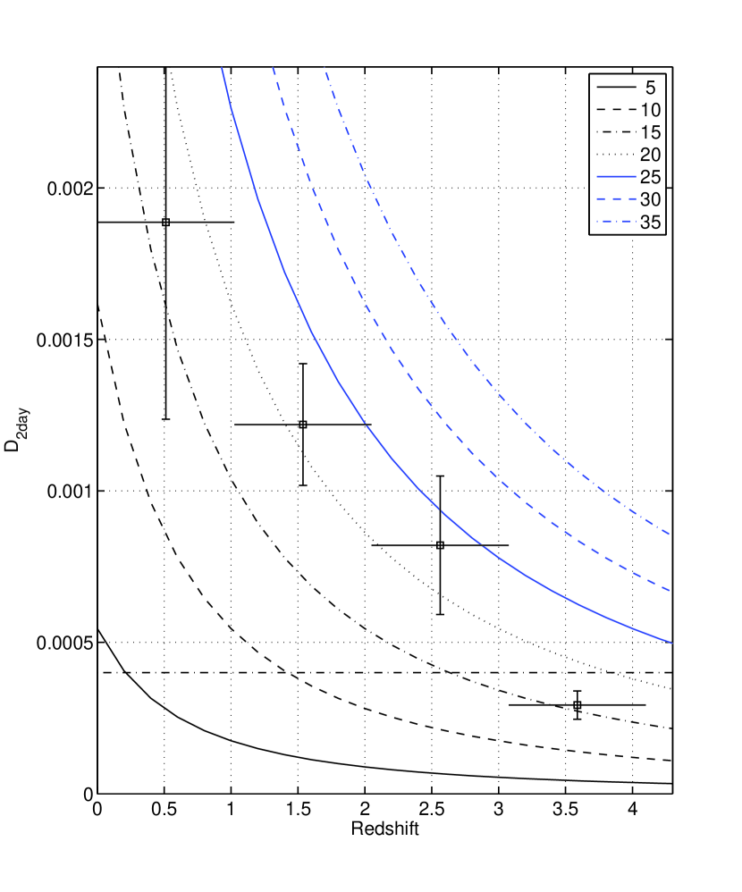
Figure 9: The data for all FSRQs averaged into 4 redshift bins. Over plotted are theoretical curves for a simple ISS model, discussed in the text, with Doppler factors as indicated in the legend. The horizontal line is at 4 $\times 10^{-4}$, which is the threshold for significant variation.

The 275 radio-selected MASIV sources with redshifts known prior to the present paper revealed that ISS of compact sources at 5 GHz decreases with redshift above $z\sim 2$ (Lovell et al., 2008). In Figure 3 of Koay et al. (2012) we considered the possible influence of a cutoff in radio power or in redshift and found that either a single cutoff beyond redshift $z$=2 explains the data, or different cutoffs in $P_{r}$ would be required for the weak and strong samples. Here we follow the simpler hypothesis of a physical model in which $D({\rm 2days})$ is governed by $S_{5GHz}$ and redshift regardless of $P_{r}$. The model is motivated by the physics of jet emission as discussed below and also by Koay et al. (2012). This model also explains why the radio weak sample has a stronger redshift dependence of $D({\rm 2days})$ compared to the radio strong sample (see Figure 9 in Koay et al., 2012).

In Figure 9 we have averaged $D({\rm 2days})$ into four redshift bins for the FSRQs alone, combining both weak and strong sources. We note that excluding the Type 2 sources increases the level of ISS in the lowest redshift bin and excluding the Type 0 sources decreases the level of ISS in the lowest redshift bin, when compared with our earlier results (Lovell et al., 2008). We also over plot the data with curves from a simple theoretical model. The model makes many assumptions and so is quite simplistic; however, it has the merit of including the most obvious cosmologically important parameters. We assume that the scattering is due to a single layer of isotropic Kolmogorov turbulence in the interstellar electron density centered at 500 pc from the Earth. We further assume that the scintillation for a point source at 5 GHz is at the transition from weak to strong scintillation. We model the compact part of the sources by a relativistic jet pointed toward the Earth emitting beamed radiation characterized by a brightness temperature in the jet frame of $T_{b0}=10^{11}$ K which delivers an observable flux density of 1 Jy. This provides a crude model for synchrotron radiation that is self-absorbed causing an upper limit in brightness. The jet is characterized by a Doppler factor $\Gamma$ which is assumed independent of $z$. The apparent brightness temperature of the source at redshift $z$ is thus given by $T_{b0}\Gamma/(1+z)$.

Since for a flux density limited sample the apparent angular diameter varies as the inverse square root of the apparent brightness temperature, the (1+$z$) reduction factor causes the apparent diameter of the compact source to increase as $\sqrt{1+z}$, which corresponds to the cosmological “angular size versus redshift” phenomenon. VLBI observers have long sought to detect this predicted increase in angular diameter with redshift, but with only partial success. For example, Gurvits et al. (1999) show angular diameters of compact radio sources that exhibit a barely significant increase beyond a redshift of about 1. We see a highly significant drop in $D({\rm 2days})$ with redshift, but a model for the ISS phenomenon is required before it can be interpreted cosmologically. An ISS model was applied to the data from the Green Bank monitoring observations by Rickett et al. (2006). However, here we have improved the model by using the formulae developed by Goodman & Narayan (2006), which explicitly include contributions from diffractive scintillations, that are important near the transition from weak to strong scintillation and were not included by Rickett et al. (2006). An understanding of $D({\rm 2days})$ is obtained by noting its asymptotic dependence $\propto\theta_{\rm source}^{-2}$ for intraday ISS. This assumes that the ISS is quenched and that its time scale is not much longer than 2 days. However, if the time scales are much longer, then $D({\rm 2days})$ drops even more steeply with $\theta_{\rm source}$. The values chosen for $T_{b0}$, $\Gamma$ and the mean flux density $S_{c}$ in the compact source enter through a single quantity $T_{b0}\Gamma/S_{c}$. Thus, while the model exhibits the expected dependence on redshift, we should also expect a wide range in this unknown quantity.

A single model curve ($\Gamma=20$) can be seen to overlap three of the four observed values within $\pm 1\sigma$. However, in the highest redshift bin, $D({\rm 2days})$ lies more than $2\sigma$ below the curve. A steeper than predicted drop in ISS with redshift could imply redshift evolution in the Doppler factor of the jets or angular broadening caused by propagation through the intergalactic medium, as mentioned by Lovell et al. (2008). However, the discrepancy shown here is not statistically strong enough and we await further redshift values from the remaining (weak sample) sources before further analysis. In fact, this discrepancy at the highest redshift bin could be linked to a steepening of the mean source spectral index with increasing redshift, coupled with the lower $D({\rm 2days})$ of steeper spectrum sources, as has been found in the dual-frequency follow-up observations (Koay et al., 2012). As noted in Section 2, the flux densities used to estimate the spectral indices for the selection of MASIV sources were non-simultaneous; and the dual-frequency follow-up observations provided more accurate estimates. Indeed any more detailed analysis must also consider the distributions in the parameters of the model rather than the single values adopted here. Nevertheless, we stress that the present work presents the strongest observational evidence to date for the predicted increase in angular size due to cosmological expansion.

6 SUMMARY

We present the optical and spectroscopic identifications of a sample of 475 flat-spectrum radio sources which are unresolved at 5 GHz (FWHM $\lesssim$ 50 mas). About half of these sources also show ISS. Our sample is divided into radio strong (S${}_{5GHz}>$ 0.3 Jy) and radio weak ( 0.06$<$ S${}_{5GHz}<$0.3 Jy) categories. For optical identification the SDSS DR5 and GSC2.3 surveys were used. About 80% of the radio strong and 60% of the radio weak sources have an optical counterpart with $R<$ 20 magnitude. Using sub-samples defined from the SDSS data indicates that the nearly complete radio strong sample ($\langle S_{\rm 5GHz}\rangle=0.9$ Jy, N=78) has median $r$-magnitude $\sim 17.9\,(r_{\rm max}\sim 22.0$), and the 70%-identified radio weak sample has $r\sim$ 18.9 ($r_{\rm max}\sim$ 22.9, $\langle S_{\rm 5GHz}\rangle=0.1$ Jy, N=95).

Spectroscopic identifications and redshifts are from the literature and from our own observations (347 sources). Spectroscopic identification of the radio strong sample is 91% complete and the weak sample is 57% complete.

The key findings can be summarized as follows:

1) The radio weak sources have flatter radio-optical spectral index than the radio strong sources.

2) Almost 80% of the MASIV sources are identified as broad line objects, $\sim$13% as BL Lacs and $\sim$7% as narrow line objects or galaxies. The spectroscopic identifications are similar for the radio strong and weak samples. Our results suggest that selecting for compact radio structure favors FSRQs and BL Lacs over other flat spectrum sources.

3) Of the scintillating sources, 25% are BL Lacs and the rest are almost exclusively broad line objects. The fraction of BL Lacs increases with the degree of persistence of ISS and 40% of the sources with most persistent ISS (scintillating at all four epochs) are BL Lac objects. This is consistent with BL Lacs being more strongly core dominated than FSRQs, and could possibly indicate relativistic jets that are pointed closer to the direction of the Earth. We confirm that $D({\rm 2days})$ depends on 5 GHz flux density, with weak sources having higher $D({\rm 2days})$ values. A similar trend is found also when broad line or weak line objects are studied separately. We found indications that the ISS properties correlate with emission line equivalent width.

4) Radio and optical luminosities of the scintillating and non-scintillating broad line sources are similar at a given redshift, suggesting intrinsically similar SEDs.

5) We find no correlation between the optical luminosity and ISS. We find a weak correlation between radio power and ISS. However at given redshift the ISS and non-ISS sources have similar radio power.

6) For broad line objects, we confirm the sharp decrease in the number of ISS sources and in the level of their ISS above a redshift $\sim$ 2. The decrease is compared to a simple model for ISS of flat spectrum radio sources with maximum brightness temperatures that are Doppler-boosted in jets pointing toward the Earth. There is reasonable agreement but more redshifts are needed for the weak radio sample. We found strong observational evidence for the predicted increase in angular size due to cosmological expansion.

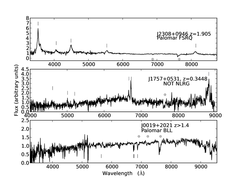
Figure 4: Example spectra of an FSRQ (Type 1), NLRG (Type 2) and BL Lac object. In the top panel the vertical bars indicate redshifted Ly$\alpha$, Si II, C IV$\lambda$1549, C III$\lambda$1909 and Mg II$\lambda$2798. In the middle panel vertical bars indicate redshifted Ne V$\lambda$3426, O II$\lambda$3730, Ne III$\lambda$3870, [O III]$\lambda\lambda$4958, 5007 and $H\alpha$. In the bottom panel the vertical bars indicate absorption lines at redshift 1.41 with Mg I$\lambda$2852, Mg II$\lambda$$\lambda$2803,2796 and Fe II$\lambda$2344. The $\oplus$-signs identify features due to the Earth’s atmosphere

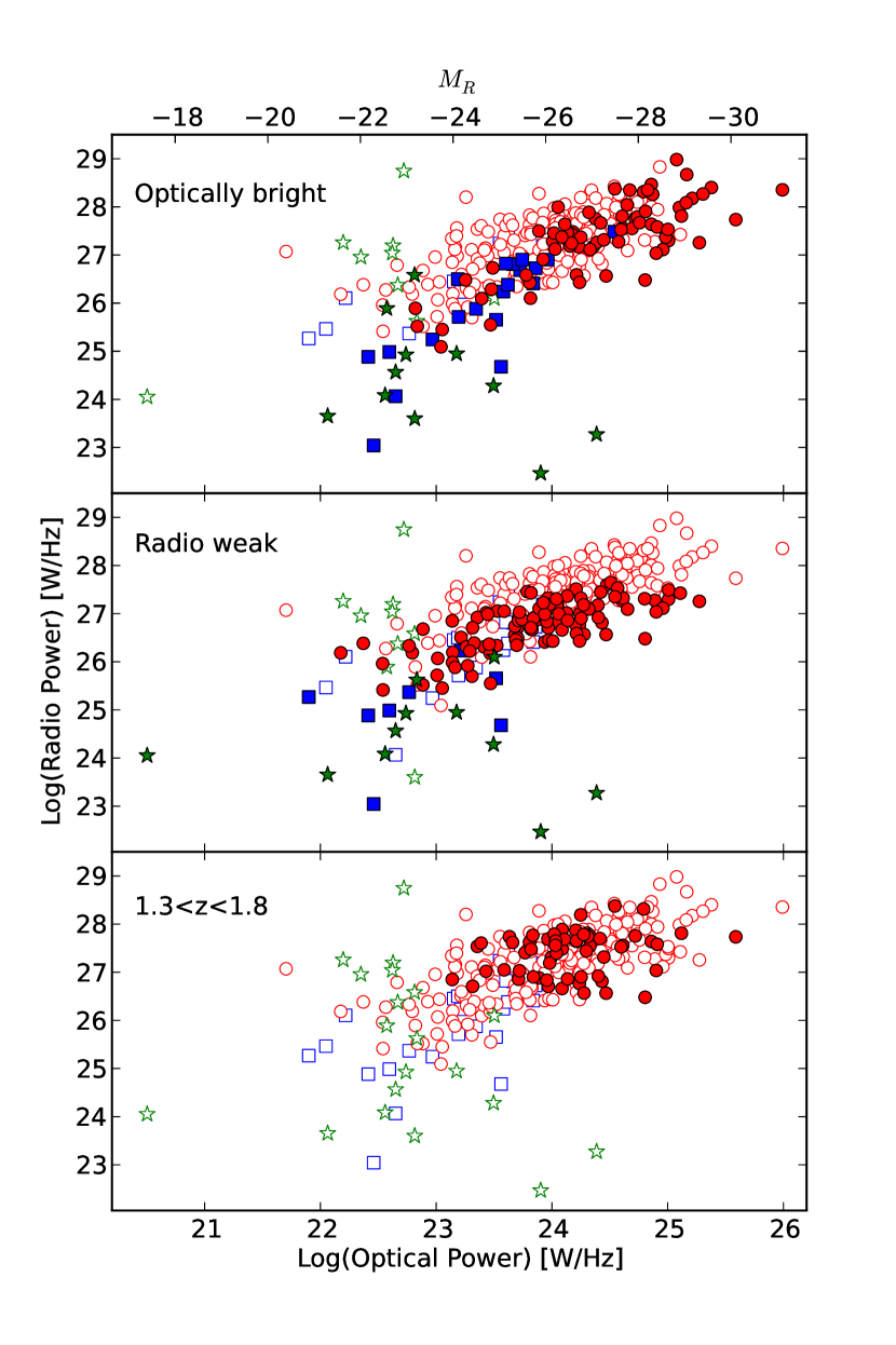
Figure 6: Optical R-band luminosity versus radio power, with FSRQ, BL Lac and AGN marked with red circles, blue squares and green stars respectively. The filled symbols show in the top panel the location of optically bright sources, in the middle panel radio weak sources and in the bottom panel redshift $1.3<z<1.8$ objects. Note the two outliers (J0248+0434 and J1141+5953) near $M_{R}$=-26, whose magnitude estimates from the USNO-B1 are too bright.

Figure 8: $D({\rm 2days})$ against redshift for the Type 1 sources. Red triangles indicate radio strong sources and blue circles radio weak sources. The horizontal thin and thick lines indicate the median $D({\rm 2days})$ for the given redshift interval for radio strong and weak samples, respectively. Type 0 objects are not shown as most of them do not have redshifts.

Table 1: Summary of the optical identification using GSC2.3 and SDSS DR5.

5GHzlimit	N	median	EF	survey
S$>$0.3Jy	193	18.2	36	GSC2.3 $F$
S$<$0.3Jy	167	19.5	79	GSC2.3 $F$
$7^{h}<RA<16^{h}$ and $\delta<$ 64
S$>$0.3Jy	62	18.25	4	SDSS $r$
S$<$0.3Jy	75	19.82	11	SDSS $r$

Note. — Columns:(1) the radio flux density limit, (2) the number of detected optical counter parts (3) the median magnitude of the sample (no galactic extinction correction) (4) non-detections (5) The survey and pass band

Table 2: MASIV Data

Source	RA	Dec	$S_{5GHz}$	Var	$D({\rm 2days})$	E(B-V)	R	Ref	$z$	Type	ID	Ref	Comment
(1)	(2)	(3)	(4)	(5)	(6)	(7)	(8)	(9)	(10)	(11)	(12)
J0005+3820	00:05:57.1755	38:20:15.168	0.61	1	0.0897	0.08	17.00	G	0.229	T1	fsrq	1
J0010+1724	00:10:33.9920	17:24:18.791	0.84	0	0.0378	0.03	16.96	G	1.601	T1	fsrq	2
J0017+5312	00:17:51.7596	53:12:19.125	0.90	2	0.4006	0.18	17.10	G	2.574	T1	fsrq	3,4
J0017+8135	00:17:08.4750	81:35:08.137	0.61	0	0.1857	0.40	15.49	G	3.387	T1	fsrq	5
J0019+2021	00:19:37.8545	20:21:45.570	1.15	1	0.0604	0.06	18.69	G	…	T0	bll	6,7
J0019+7327	00:19:45.7871	73:27:30.019	0.44	1	0.3216	0.32	17.48	G	1.781	T1	fsrq	8

Note. — Columns are as follows (1) IAU name (J2000.0), (2)R.A.(J2000.0), (3)Decl.(J2000.0) (4) first epoch MASIV 5GHz flux density, (5) The number of epochs of variability based on visual classification, where ’C’ indicates secondary calibrators, (6) Structure function $D({\rm 2days})$, (7) Galactic extinction, (8) R-magnitude, (9) Reference; G=GSC2.3, S=SDSS DR5, U=USNO-B R2 (10) Redshift, (11) Spectral type (12) Spectroscopic identification, (13) Reference for redshift and spectroscopic identification, (14) Comment

References: (1) Stickel & Kuehr (1994) (2) Wills & Wills (1976), (3) Sargent et al. (1989), (4) Kuhr et al. (1983), (5) Sowards-Emmerd et al. (2005), (6) Chu et al. (1986), (7) Palomar 2007 this paper, (8) Lawrence et al. (1986)

Table 1 is published in its entirety in the electronic edition of ¡¿, A portion is shown here for guidance regarding its form and content.

Table 3: Objects with single emission line from our data (that have an ambiguous identification). The range indicates the useful wavelength range of the spectrogram.

Source	Line	Range	S/Nmax
	Å	Å	per pixel
J0213+3652	4179	3500-5000	02
J0342+3859	5453	4150-7500	15
J1316+6927	5675	4500-7500	03
J1711+6853	5660	3900-8500	08
J1953+3537	5125	5200-7500	10
J2012+5308	3967	3950-7500	06

Table 4: Summary of the spectroscopic identification. The third and fourth column indicates the number of sources in the radio strong and radio weak samples, respectively.

Type	Spect id	Strong	Weak
Type 0	BLL	037	011
	BLL?		005
	PEG		006
Type 1	FSRQ	155	107
	FSRQ?	001
	Sy 1		002
	Sy 1/BLRG	001
	NLSy1	001
	NLQSO	002
	Sy1.5/LINER	001
Type 2	Sy2	003	002
	Sy2?		001
	NLRG	005	001
	LINER	001	001
	HII?		001
	galaxy		003
Single line objects		001	005

Table 5: Classification break down of the radio strong and weak samples including the secondary calibrators. The ’SDSS sample’ source distributions are in column four and five.

type	Nfull	%	NSDSS	%
Radio strong sources
Type 0	37	18$\pm$3%	19	24$\pm$6 %
Type 1	162	78$\pm$6%	57	72$\pm$10%
Type 2	9	4$\pm$1%	2	3$\pm$2 %
Radio weak sample
Type 0	22	16$\pm$3%	8	14$\pm$5%
Type 1	108	78$\pm$7%	46	78$\pm$11%
Type 2	9	6$\pm$2%	5	8$\pm$4%

Note. — The errors are Poissonian.

Table 6: Summary of some flat radio spectrum AGN surveys. Note, the PEGs in CBS and MASIV are included in the “other AGN” as is the case with CGRaBS and DXRBS.

Survey	5 GHz limit	R-mag	FSRQ	BL Lac	other AGN	Comment
	$mJy$		%	%	%
CBS	30	17.5	45	21	34
CBS rb	65:	17.5	51	20	29	MASIV 5 GHz limit
CGRaBS	65	23.7	88	10	2	Selection by $Figure\,of\,Merit$
DXRBS	50	24.0	80	12	8	some steep spectrum sources
MASIV	60	23.1	78	15	7	Selection by 8.4 GHz
MASIV ob	60	17.5:	64	24	12	Optically bright CBS limit
MASIV ISS	60	21.3	64	34	2	Persistent IDV sources, IDV3, 4
MASIV SDSS	60	21.7	75	18	7	SDSS sample

Note. — Columns:(1) the name of the sample, (2) 5 GHz radio flux density limit for faintest objects, (3) optical magnitude limit or the faintest detected objects, (4) the fraction of broad line objects, (5) the fraction of BL Lac objects (6) the fraction of other spectral type objects, mostly narrow line objects.

The colon indicates MASIV radio flux density limit for the “CBS rb”, and CBS optical limit for “MASIV ob”. Note, the DXRBS includes steep radio spectrum sources as well (Landt et al., 2001).

Table 7: Median $D({\rm 2days})$ of the subsamples selected by optical spectral type and 5 GHz flux density. The First column indicates optical spectral type, followed by the median $D({\rm 2days})$ and the number of objects.

Type	$D({\rm 2days})\times$1000	N	$D({\rm 2days})\times$1000	N
	$S_{5GHz}>0.3Jy$		$S_{5GHz}<0.3Jy$
0	0.701	31	2.35	22
1	0.335	143	0.868	108
2	0.193	6	0.44	9
Type 1 $z<1.4$ sources
1	0.346	79	1.27	54

Table 8: Number of sources and the fractions of “variable” MASIV epochs for the three optical spectral types. The first column indicates the number variable in epochs and the next columns show the fraction of sources in each group with the number of sources in parentheses.

Sample	Type 0		Type 1		Type 2
IDV	strong	weak	strong	weak	strong	weak
0	13% (4)	18%   (4)	36% (51)	36%(39)	5	7
1	19% (6)	18%   (4)	24% (34)	15%(16)	1	1
2	13% (4)	(0)	24% (34)	17%(18)	0	0
3	29% (9)	18%   (4)	8% (12)	18%(19)	0	1
4	26% (8)	46% (10)	8% (12)	15%(16)	0	1

Table 9: Redshift, core radio power and optical luminosity, excluding secondary calibrators. The IDV0, IDV1, etc. indicates the number of epochs of variability (Lovell et al., 2008).

	Strong sources				Weak sources
Sample	N	$<z>$	log($P_{r}$)	$M_{R}$	N	$<z>$	log($P_{r}$)	$M_{R}$
			$Wm^{-2}$				$Wm^{-2}$
Type 0	16	0.4$\pm$0.3	26.6$\pm$0.6	-25.2$\pm$1.1	10	0.2$\pm$0.1	25.0$\pm$0.8	-23.6$\pm$1.3
Type 1	142	1.3$\pm$0.7	27.6$\pm$0.6	-26.4$\pm$1.6	108	1.4$\pm$0.8	26.8$\pm$0.5	-25.9$\pm$1.6
Type 2	6	0.4$\pm$0.3	26.7$\pm$1.3	$\cdots$	9	0.1$\pm$0.2	24.1$\pm$1.1	$\cdots$
	Type 1
$D({\rm 2days})$$>4\times 10^{-4}$	59	1.2$\pm$0.6	27.5$\pm$0.6	-26.2$\pm$1.4	76	1.3$\pm$0.7	26.7$\pm$0.5	-25.7$\pm$1.5
$D({\rm 2days})$$<4\times 10^{-4}$	83	1.4$\pm$0.7	27.7$\pm$0.5	-26.7$\pm$1.6	32	1.8$\pm$1.0	27.0$\pm$0.5	-26.7$\pm$1.4
	1.0 $<z<$ 1.8
$D({\rm 2days})$$>4\times 10^{-4}$	24	1.4$\pm$0.2	27.5$\pm$0.2	-26.4$\pm$1.0	29	1.3$\pm$0.2	26.7$\pm$0.2	-26.0$\pm$1.2
$D({\rm 2days})$$<4\times 10^{-4}$	35	1.4$\pm$0.2	27.6$\pm$0.2	-26.4$\pm$1.3	10	1.3$\pm$0.3	26.8$\pm$0.2	-25.7$\pm$1.0
	Type 1
ISS (IDV234)	58	1.2$\pm$0.7	27.5$\pm$0.6	-26.3$\pm$1.4	53	1.2$\pm$0.6	26.7$\pm$0.5	-25.4$\pm$1.4
IDV0	50	1.4$\pm$0.8	27.7$\pm$0.6	-26.7$\pm$1.8	39	1.9$\pm$1.0	27.1$\pm$0.5	-26.5$\pm$1.6
IDV1	34	1.3$\pm$0.6	27.5$\pm$0.5	-26.3$\pm$1.3	16	1.4$\pm$0.7	26.8$\pm$0.4	-26.0$\pm$1.3
IDV2	34	1.5$\pm$0.7	27.6$\pm$0.6	-26.4$\pm$1.5	18	1.3$\pm$0.7	26.7$\pm$0.5	-26.0$\pm$1.3
IDV3	12	1.0$\pm$0.5	27.4$\pm$0.6	-25.9$\pm$1.2	19	1.1$\pm$0.7	26.6$\pm$0.6	-25.0$\pm$1.4
IDV4	12	1.4$\pm$0.7	27.6$\pm$0.4	-26.5$\pm$1.3	16	1.2$\pm$0.5	26.7$\pm$0.4	-25.3$\pm$1.4

Note. — Columns: (1) the sub-sample, (2) Number of objects, (3) Median redshift, (4) Median of the Log radio power with standard deviation, (5) Median absolute magnitude with standard deviation, (6)-(9) same as Cols. (2)-(5).

Appendix A COMMENTS ON ARCHIVAL REDSHIFTS

After careful inspection three objects with archival redshift were rejected. In addition, unreliable redshifts have been proposed for ten BL Lac objects and four objects with adopted, but uncertain redshift or spectroscopic identification. We briefly discuss these here.

J0200+0322: Fricke et al. (1983) reported redshift, $z$=0.765, based on a single (Mg II$\lambda$2798) line at 4920Å. Their spectrum had the wavelength range from 4200-7100Å  where for a typical QSO spectrum a single broad line can be detected at $z\sim$ 0.8 (Mg II) or 1.6 (C III]).
J0204+1514: Stickel et al. (1996) reported $z$=0.833 based on two narrow emission lines. Later Perlman et al. (1998) found more lines and a better fit for $z$=0.405 and they classified this object as an FSRQ, which we adopted for this work. However this object should be re-observed in order to secure the spectroscopic identification.
J0406+2511: Hook et al. (1996) assumed the single line at 6260Å  to be [O II]$\lambda$3727, at $z$=0.68. Their data has a wavelength range from 5200-9100Å, however the red and blue ends are very noisy, reducing the useful range to 5800-8500Å. If the redshift is indeed 0.68, H$\beta$ should be around 8150Å, and/or [O III]$\lambda$5007 around 8410Å, which are not seen.
J0449+1121: von Montigny et al. (1995) reported $z$=1.27, however Halpern et al. (2003) found featureless spectrum. Thus we adopted a BL Lac identification for this source.
J0738+1742: NED reports $z=$ 0.424. However, this is the redshift of intervening MgII absorption feature, i.e. $z\gtrsim$ 0.43 (Rector & Stocke (2001) and references therein).
J0745+1011: We adopted the redshift from Best et al. (2003) who measured $z$=2.624, however, Labiano et al. (2007) could not confirm this. If the redshift is correct the radio power is 4$\times$10²⁸W/Hz and an outlier in the $M_{R}$-Log($P$)-plot (Figure 6). This object should be re-observed.
J0753+5352: This source has featureless optical spectrum and the redshift has a lower limit of 0.2 based on imaging data (Stickel & Kuehr, 1993).
J0818+4222: This is a radio source with featureless optical spectrum and has no reliable redshift available (Rector & Stocke (2001) and references therein).
J0929+5013: The SDSS redshift is uncertain as there are no obvious emission lines.
J1150+2417: This object has a featureless optical spectrum Rector & Stocke (2001, and references therein).
J1309+1154 This object has a featureless optical spectrum by Lynds & Wills (1972) and SDSS. Note that this object has SDSS DR5 redshift of 0.3852 and SDSS DR 8 redshift of 2.601.
J1446+1721: The redshift of this FSRQ is uncertain as Sowards-Emmerd et al. (2005) reported, $z$=0.102, however Healey et al. (2008) reported $z$=1.026. For this work we adopt FSRQ classification with unknown redshift.
J1502+3350: White et al. (2000) report featureless spectrum for this object. Note that the SDSS DR6 suggest $z$=2.222, however the spectrum appears featureless.
J1602+3326: The redshift is based on optical magnitude (Snellen et al., 2000) using the GPS galaxy Hubble diagram (Stanghellini et al., 2005).
J1648+2141 The SDSS spectrum is featureless, however the SDSS DR6 suggest $z$=1.085.
J1649+7442: This redshift is from Appenzeller et al. (1998) from the spectrum with a wavelength range from 4000 to 7000/9000Å. The redshift is based on a single line at 6658Å  which is assumed to be Mg II$\lambda$2798 at $z$=1.378. At this redshift, one would expect to see C III]$\lambda$1909 at 4532Å, however if the line was C III] or H$\beta$ one would expect to see C IV at $\sim$5392Å  or [O III] near 6870Å. The redshift is adopted, but needs to be confirmed.
J1719+1745: Sowards-Emmerd et al. (2005), reported $z$=0.173. However Shaw et al. (2009) find featureless spectrum and they estimate redshift to be $>$0.58. This source is classified as a BL Lac object without known redshift.

Appendix B TRANSFORMATION FROM GSC2.3 TO LANDOLT SYSTEM

In order to transform the GSF2.3 magnitudes to the Landolt (2009) system, we obtained $JFN$ magnitudes from the Landolt standard stars. We included only stars with four or more measurements by Landolt, then plotted $J-B$, $F-R$ and $N-I$ and removed outliers. Least squares polynomial fit resulted following transformations:

$$B_{GSC}=J+0.18(J-F)-0.08,$$ (B1)

$$R_{GSC}=F[-0.085(F-N)+0.04],$$ (B2)

$$I_{GSC}=N[+0.066(F-N)-0.02].$$ (B3)

The terms in square brackets for $R_{GSC}$ and $I_{GSC}$ are from the best least-squares fit, however the fit is improved only marginally, hence we have omitted the color term. The root mean squared error for the BRI-conversions are 0.10, 0.11 and 0.11, respectively.

The $B_{GSC}$ transformation is valid for the $(J-F)$-colors from -0.5 to 2.5 and $R_{GSC}$, $I_{GSC}$ for the $(F-N)$-color range from -0.4 to 1.4.

Appendix C NOTES ON INDIVIDUAL OBJECTS

In this appendix, we discuss some of our spectroscopic follow-up targets. For the narrow line objects we report the EW of the strongest line.

J0019+2021 BL Lac classification is from Chu et al. (1986) who found no strong emission lines. Our DBSP data (S/N$\lesssim$35) shows absorption system at $z$=1.41 with Mg I$\lambda$2852, Mg II$\lambda$$\lambda$2803,2796, (Fe II$\lambda$2344) and a possible absorption system at $z$=2.274 (Figure 4).
J0150+2646 The DBSP (07-2007) and NOT (8-2004) spectrum are featureless with S/N$\lesssim$14 and S/N$\lesssim$8, respectively. Thus, this source is tentatively identified as a BL Lac object.
J0509+0541 Halpern et al. (2003) reported featureless spectrum from several observations. Our high S/N ($>$130) data is featureless showing only galactic absorption lines and unidentified absorption at 4276$\AA$.
J0800+4854 Our data show strong absorption at the C IV$\lambda$1549- and Ly$\alpha$-lines and also the He II$\lambda$1640-line is easily detected.
J1118+2922 This low redshift object has two easily detected narrow emission lines at $\lambda$3998Å   and $\lambda$7038Å, identified as [O II]$\lambda$3727 and H$\alpha$ at redshift of 0.072. The line ratios suggest HII region or Liner classification.
J1352+3603 We detect narrow [O III]$\lambda$$\lambda$4958, 5007 and [O II]$\lambda$3727 lines at $z$=0.3057 with, M_B=-21.5, (M_R=-23.0), C=42%, EW([O II])=20Å   and noisy EW(H$\alpha$)$\sim$ 37Å. The source is classified as PEG based on the Ca-break and line EW. On the other hand, based on the classification scheme of Landt et al. (2004), this is a strong-lined source.
J1442+0625 Our data show a single line at 4753Å, with continuum from 4800-7500Å  (S/N$\lesssim$10). Our tentative identification is Mg II$\lambda$2798-line at $z$=0.698. If this line would be C III] at $z$=1.49 we would expect to see Mg II$\lambda$2798 at about 7000Å  which is not detected.
J1444+0257 This object has a featureless spectrum from 4500 to 7500Å  with S/N$\lesssim$5, possibly a BL Lac object
J1444+1632 We detect a single line at 5688Å  with noisy continuum (S/N $\lesssim$3) and tentative line at 7247Å, these are identified as Ly$\alpha$ and C IV$\lambda$1549, which would indicate $z$=3.7.
J1505+0326 This object has been classified as FSRQ in CGRaBS (Healey et al., 2008). Our NOT data confirms the CGRaBS and SDSS redshift. However reanalyzing the SDSS data and based on the NOT data the rest frame line widths are less than 2000km/s indicating NLSy1 classification.
J1651+0129 Our DBSP data shows a possible line at 7128Å  with the continuum S/N$\lesssim$7. As we are not able to identify the line or spectrum, this target is not included to the analysis.
J1718+4448 The DBSP red spectrum show no obvious lines from 5300 to 8300Å  with S/N $\lesssim$ 5, possibly a BL Lac object.
J1728+1931 We detect narrow ([O II]$\lambda$3727), [O III]$\lambda$$\lambda$4958, 5007 and a noisy [O I]$\lambda$6300 lines at $z$=0.1759, with [O III]$\lambda$5007/H$\beta$$>$3, EW([O II])=13Å, M_B=-21.1, (M_R=-24.2) and C=42%. The H$\alpha$-line is noisy, however it appears to be narrow. This is border line object between strong and weak lined sources using Landt et al. (2004) classification. We tentatively classify this as a Sy2-type object.
J1734+3857 Stickel et al. (1989) classification for this source is an FSRQ at $z$=0.97 based on a single broad emission line which was assumed to be Mg II$\lambda$2798 (EW(Mg II)=15.3Å, observed) Our data shows also only a single line at 5535Å  assumed to be Mg II at $z$=0.97 with the EW=4.2Å, hence BL Lac classification.
J1739+4737 This is a BL Lac-object with featureless spectrum (Scarpa et al., 2000). Our DBSP data show no lines with S/N$\lesssim$20
J1742+5945 This object has a featureless spectrum Laurent-Muehleisen et al. (1998), and the redshift ($z$=0.4) is based on a detection of the host galaxy (Nilsson et al., 2003). Our NOT spectrum (07-2006) shows no lines from 4000 to 7500 Å  with S/N$\lesssim$25.
J1747+4658 This source has no emission line redshift. Vermeulen et al. (1996) reported an intervening Mg II absorption line system at $z$=1.484, which, by some authors, has been adopted as the source redshift. Our NOT spectrum (Grism 6) from 4000 to 5500Å  with S/N$<$6 is featureless.
J1757+0531 Narrow emission lines, [O II]$\lambda$3727 and [O III]$\lambda$$\lambda$4958, 5007 at $z$=0.34482 are clearly visible and so is a noisy strong H$\alpha$ feature at the red end of the spectrogram. The line and continuum properties suggest Type 2 identification: [O III]$\lambda$5007/H$\beta$$>$3,   M_R=-23.2,   EW([O III]$\lambda$5007)=37Å   and C=28%. However the continuum is rather noisy, (S/N$\lesssim$8) and weak broad emission lines might have been undetected (Figure 4). Tentative spectroscopic identification is NLRG, however, based on Fig. 8 and 9 of Caccianiga et al. (2008) this object could be a Type 1 object with the AGN core diluted by the host galaxy.
J1832+1357 Our data confirms the CGRaBS (Healey et al., 2008) redshift. We detect also some absorption features in C IV$\lambda$1549-line
J1848+3219 Sowards-Emmerd et al. (2005) reported this source as an FSRQ at $z$=0.798. Our data shows a strong line at 5035Å, a noisy narrow line at 6703Å  (identified as Mg II$\lambda$2798 and [O II]$\lambda$3727, respectively) and no strong lines in 3600-5000 and 5100-7500Å  with S/N$\lesssim$17, supporting the literature identification and redshift.
J1905+1943 A strong broad line is detected at 5106Å  and a tentative broad line at 6267Å, suggesting $z=$2.3.
J1950+0807 From the DBSP data we detect narrow [O II]$\lambda$3727, [O III]$\lambda$$\lambda$4958, 5007 and broad H$\alpha$-lines at $z$=0.2964, with M_R=-22.8, M_B=-20.7 and EW([O III]$\lambda$5007)=-48Å, suggesting Sy1.9 classification.
J2023+5427 The redshift 1.48 is measured from Mg II$\lambda$2798 and C III]$\lambda$1909-lines. In addition we detect MgI(2852), MgII(2803,2796), FeII(2387,2600) and FeII(2383,2344) absorption lines at $z$=1.415
J2130+0339 From the DBSP data we detect narrow lines [O II]$\lambda$3727 and [O III]$\lambda$$\lambda$4958, 5007 at $z$=0.653, with EW([O III]$\lambda$5007)=140Å, M${}_{R}>$-22.5 and C=31%, suggesting Type 2 identification. Note, this source is not detected in the GSC2.3.
J2155+0916 This object is tentatively identified as a BL Lac object. Our NOT spectrum is featureless from 4500 to 7500Å  with S/N$\lesssim$20, however if the redshift is $\sim$0.6, both Mg II$\lambda$2798 and H$\beta$-lines will be outside the spectrogram.
J2201+5048 We confirm the Sowards-Emmerd et al. (2005) redshift, 1.899 and in addition we detect Mg II-absorption system at $z$=1.3822 with Mg I$\lambda$2852, Mg II$\lambda$$\lambda$2803,2796, Fe II$\lambda$2344,2374,2383, however this source was rejected from the Lovell et al. (2008) analysis due to evidence of source structure, hence not included to the analysis.
J2203+1725 Smith et al. (1977) classified this source as a FSRQ based on strong C III]$\lambda$1909- and Mg II$\lambda$2798-lines at $z$=1.076. Our data shows a single line at 5811Å  with EW(Mg II)=3.3Å  and S/N$\lesssim$60 around the line, hence BL Lac object classification.
J2212+2759 This is a BL Lac object, with no detected emission lines, based on our DBSP data (07-2007) with S/N$\lesssim$45 and NOT data (07-2005) with S/N$\lesssim$18.
J2230+6946 We confirm the Healey et al. (2008) (CGRaBS) redshift.
J2237+4216 An emission line is detected at 5655Å  and this is the only emission line between 4500 and 7500Å, suggesting Mg II identification.
J2241+4120 Henstock et al. (1997) and Sowards-Emmerd et al. (2005) classified this as a BL Lac object. Our DBSP data (07-2007) with S/N$\lesssim$60 and NOT data (07-2005) from 4000 to 7500Å  with S/N$\lesssim$30 confirm this.
J2242+2955 A strong broad line is detected at 4102Å  and a tentative broad line at 5013Å, suggesting $z=$1.7.
J2258+0516 We detected a strong absorption feature at the centre of the C IV$\lambda$1549-line and Ly$\alpha$ line is almost fully absorbed.
J2303+1431 This is a BL Lac object with featureless spectrum. Our DBSP spectrum (07-2007) has S/N$\lesssim$25 and NOT spectrum (07-2006) S/N$\lesssim$8.
J2315+8631 A broad line at 5273Å  (Mg II$\lambda$2798) is visible in our DBSP (08-2007) and NOT (07-2006) spectrum. This is the only strong emission line between 3700 and 8500Å  (S/N$\lesssim$30) , hence a tentative redshift of $z$=0.88.
J2325+3957 Shaw et al. (2009) reported a featureless spectrum with intervening Mg II$\lambda$2798 and FeII absorption features at $z$=1.04. Our DBSP data (07-2007) shows no emission lines. However, we detect absorption features which are identified as Mg I$\lambda$2852, Mg II$\lambda\lambda$2803,2796, Fe II$\lambda$2600 (and Fe II$\lambda$2344) at $z$=0.4695 and Mg II$\lambda\lambda$2803,2796, Fe II$\lambda$2600 at $z$=0.4156 with the continuum S/N up to $\sim$25. We also detected an absorption feature at 5757Å  possibly Mg II$\lambda$2798 at $z$=1.04, but not the expected Fe II feature at 5353Å. The 4119Å  feature, Mg II$\lambda$2803 at $z$=0.4695, is also visible from the NOT spectrum (07-2006).

References

- Abdo et al. (2009) Abdo A.A., Ackermann M., Ajello M., et al., 2009, ApJS 183, 46
- Adelman-McCarthy et al. (2007) Adelman-McCarthy J.K., Agüeros M.A., Allam S.S., et al., 2007, ApJS 172, 634
- Appenzeller et al. (1998) Appenzeller I., Thiering I., Zickgraf F., et al., 1998, ApJS 117, 319
- Avni et al. (1980) Avni Y., Soltan A., Tananbaum H., Zamorani G., 1980, ApJ 238, 800
- Begelman et al. (1994) Begelman M.C., Rees M.J., Sikora M., 1994, Astrophys. J., Lett. 429, L57
- Best et al. (2003) Best P.N., Peacock J.A., Brookes M.H., et al., 2003, MNRAS 346, 1021
- Bignall et al. (2003) Bignall H.E., Jauncey D.L., Lovell J.E.J., et al., 2003, ApJ 585, 653
- Bignall et al. (2006) Bignall H.E., Macquart J.P., Jauncey D.L., et al., 2006, ApJ 652, 1050
- Browne et al. (1998) Browne I.W.A., Wilkinson P.N., Patnaik A.R., Wrobel J.M., 1998, MNRAS 293, 257
- Caccianiga et al. (2002a) Caccianiga A., Maccacaro T., Wolter A., et al., 2002a, ApJ 566, 181
- Caccianiga et al. (2002b) Caccianiga A., Marchã M.J., Antón S., et al., 2002b, MNRAS 329, 877
- Caccianiga & Marchã (2004) Caccianiga A., Marchã M.J.M., 2004, MNRAS 348, 937
- Caccianiga et al. (2008) Caccianiga A., Severgnini P., Della Ceca R., et al., 2008, A&A 477, 735
- Chonis & Gaskell (2008) Chonis T.S., Gaskell C.M., 2008, AJ 135, 264
- Chu et al. (1986) Chu Y.Q., Zhu X.F., Butcher H., 1986, Chinese Astron. Astrophys.10, 196
- Condon et al. (1998) Condon J.J., Cotton W.D., Greisen E.W., et al., 1998, AJ 115, 1693
- Dennett-Thorpe & de Bruyn (2002) Dennett-Thorpe J., de Bruyn A.G., 2002, Nature415, 57
- Dennett-Thorpe & de Bruyn (2003) Dennett-Thorpe J., de Bruyn A.G., 2003, A&A 404, 113
- Fricke et al. (1983) Fricke K.J., Kollatschny W., Witzel A., 1983, A&A 117, 60
- Giommi et al. (2012) Giommi P., Padovani P., Polenta G., et al., 2012, MNRAS 420, 2899
- Gonçalves & Serote Roos (2004) Gonçalves A.C., Serote Roos M., 2004, A&A 413, 97
- Goodman & Narayan (2006) Goodman J., Narayan R., 2006, ApJ 636, 510
- Gurvits et al. (1999) Gurvits L.I., Kellermann K.I., Frey S., 1999, A&A 342, 378
- Halpern et al. (2003) Halpern J.P., Eracleous M., Mattox J.R., 2003, AJ 125, 572
- Healey et al. (2008) Healey S.E., Romani R.W., Cotter G., et al., 2008, ApJS 175, 97
- Healey et al. (2007) Healey S.E., Romani R.W., Taylor G.B., et al., 2007, ApJS 171, 61
- Heckman et al. (1995) Heckman T., Krolik J., Meurer G., et al., 1995, ApJ 452, 549
- Heeschen (1984) Heeschen D.S., 1984, AJ 89, 1111
- Heeschen et al. (1987) Heeschen D.S., Krichbaum T., Schalinski C.J., Witzel A., 1987, AJ 94, 1493
- Heeschen & Rickett (1987) Heeschen D.S., Rickett B.J., 1987, AJ 93, 589
- Henstock et al. (1997) Henstock D.R., Browne I.W.A., Wilkinson P.N., McMahon R.G., 1997, MNRAS 290, 380
- Ho et al. (1995) Ho L.C., Filippenko A.V., Sargent W.L., 1995 98, 477
- Hook et al. (1996) Hook I.M., McMahon R.G., Irwin M.J., Hazard C., 1996, MNRAS 282, 1274
- Jauncey et al. (2001) Jauncey D.L., Kedziora-Chudczer L., Lovell J.E.J., et al., 2001, Ap&SS 278, 87
- Jauncey et al. (2000) Jauncey D.L., Kedziora-Chudczer L., Lovell J.E.J., et al., 2000, In: H. Hirabayashi,P.G. Edwatds & D.W. Murphy (ed.) Astrophysical Phenomena Revealed by Space VLBI, Vol. 300. Institute of Space and Astronautical Science, p.147
- Jauncey & Macquart (2001) Jauncey D.L., Macquart J., 2001, A&A 370, L9
- Kedziora-Chudczer et al. (1997) Kedziora-Chudczer L., Jauncey D.L., Wieringa M.H., et al., 1997, Astrophys. J., Lett. 490, L9+
- Koay et al. (2012) Koay J.Y., Macquart J.P., Rickett B.J., et al., 2012, ApJ 756, 29
- Koay et al. (2011) Koay J.Y., Macquart J.P., Rickett B.J., et al., 2011, AJ 142, 108
- Krichbaum et al. (2002) Krichbaum T.P., Kraus A., Fuhrmann L., et al., 2002, Publications of the Astronomical Society of Australia 19, 14
- Kuhr et al. (1983) Kuhr H., Liebert J.W., Strittmatter P.A., et al., 1983, ApJ 275, L33
- Labiano et al. (2007) Labiano A., Barthel P.D., O’Dea C.P., et al., 2007, A&A 463, 97
- Landolt (1992) Landolt A.U., 1992, AJ 104, 340
- Landolt (2009) Landolt A.U., 2009, AJ 137, 4186
- Landt et al. (2004) Landt H., Padovani P., Perlman E.S., Giommi P., 2004, MNRAS 351, 83
- Landt et al. (2001) Landt H., Padovani P., Perlman E.S., et al., 2001, MNRAS 323, 757
- Lasker et al. (2008) Lasker B.M., Lattanzi M.G., McLean B.J., et al., 2008, AJ 136, 735
- Laurent-Muehleisen et al. (1998) Laurent-Muehleisen S.A., Kollgaard R.I., Ciardullo R., et al., 1998, ApJS 118, 127
- Lawrence et al. (1986) Lawrence C.R., Pearson T.J., Readhead A.C.S., Unwin S.C., 1986, AJ 91, 494
- Lister et al. (2009) Lister M.L., Aller H.D., Aller M.F., et al., 2009, AJ 137, 3718
- Lister et al. (2001) Lister M.L., Tingay S.J., Preston R.A., 2001, ApJ 554, 964
- Lovell et al. (2003) Lovell J.E.J., Jauncey D.L., Bignall H.E., et al., 2003, AJ 126, 1699
- Lovell et al. (2008) Lovell J.E.J., Rickett B.J., Macquart J., et al., 2008, ApJ 689, 108
- Lynds & Wills (1972) Lynds R., Wills D., 1972, ApJ 172, 531
- Macquart et al. (2000) Macquart J., Kedziora-Chudczer L., Rayner D.P., Jauncey D.L., 2000, ApJ 538, 623
- Marchã et al. (2001) Marchã M.J., Caccianiga A., Browne I.W.A., Jackson N., 2001, MNRAS 326, 1455
- Monet et al. (2003) Monet D.G., Levine S.E., Canzian B., et al., 2003, AJ 125, 984
- Myers et al. (2003) Myers S.T., Jackson N.J., Browne I.W.A., et al., 2003, MNRAS 341, 1
- Narayan (1992) Narayan R., 1992, Royal Society of London Philosophical Transactions Series A 341, 151
- Nilsson et al. (2003) Nilsson K., Pursimo T., Heidt J., et al., 2003, A&A 400, 95
- Ojha et al. (2010) Ojha R., Kadler M., Böck M., et al., 2010, A&A 519, A45+
- Padovani et al. (2007) Padovani P., Giommi P., Landt H., Perlman E.S., 2007, ApJ 662, 182
- Patnaik et al. (1992) Patnaik A.R., Browne I.W.A., Wilkinson P.N., Wrobel J.M., 1992, MNRAS 254, 655
- Perlman et al. (1998) Perlman E.S., Padovani P., Giommi P., et al., 1998, AJ 115, 1253
- Pier et al. (2003) Pier J.R., Munn J.A., Hindsley R.B., et al., 2003, AJ 125, 1559
- Readhead (1994) Readhead A.C.S., 1994, ApJ 426, 51
- Rector & Stocke (2001) Rector T.A., Stocke J.T., 2001, AJ 122, 565
- Rickett et al. (2006) Rickett B.J., Lazio T.J.W., Ghigo F.D., 2006, ApJS 165, 439
- Rickett et al. (2001) Rickett B.J., Witzel A., Kraus A., et al., 2001, Astrophys. J., Lett. 550, L11
- Sargent et al. (1989) Sargent W.L.W., Steidel C.C., Boksenberg A., 1989, ApJS 69, 703
- Sbarufatti et al. (2005) Sbarufatti B., Treves A., Falomo R., et al., 2005, AJ 129, 559
- Scarpa et al. (2000) Scarpa R., Urry C.M., Falomo R., et al., 2000, ApJ 532, 740
- Schlegel et al. (1998) Schlegel D.J., Finkbeiner D.P., Davis M., 1998, ApJ 500, 525
- Sesar et al. (2006) Sesar B., Svilković D., Ivezić Ž., et al., 2006, AJ 131, 2801
- Shaw et al. (2009) Shaw M.S., Romani R.W., Healey S.E., et al., 2009, ApJ 704, 477
- Smith et al. (1977) Smith H.E., Burbidge E.M., Baldwin J.A., et al., 1977, ApJ 215, 427
- Snellen et al. (2000) Snellen I.A.G., Schilizzi R.T., Miley G.K., et al., 2000, MNRAS 319, 445
- Sowards-Emmerd et al. (2005) Sowards-Emmerd D., Romani R.W., Michelson P.F., et al., 2005, ApJ 626, 95
- Sowards-Emmerd et al. (2004) Sowards-Emmerd D., Romani R.W., Michelson P.F., Ulvestad J.S., 2004, ApJ 609, 564
- Stanghellini et al. (2005) Stanghellini C., O’Dea C.P., Dallacasa D., et al., 2005, A&A 443, 891
- Stickel et al. (1989) Stickel M., Fried J.W., Kuehr H., 1989, A&AS 80, 103
- Stickel & Kuehr (1993) Stickel M., Kuehr H., 1993, A&AS 101, 521
- Stickel & Kuehr (1994) Stickel M., Kuehr H., 1994, A&AS 103, 349
- Stickel et al. (1996) Stickel M., Rieke G.H., Kuehr H., Rieke M.J., 1996, ApJ 468, 556
- Stocke et al. (1985) Stocke J.T., Liebert J., Schmidt G., et al., 1985, ApJ 298, 619
- Urry & Padovani (1995) Urry M., Padovani P., 1995, PASP 107, 803
- Verdoes Kleijn et al. (2002) Verdoes Kleijn G.A., Baum S.A., de Zeeuw P.T., O’Dea C.P., 2002, AJ 123, 1334
- Vermeulen et al. (1996) Vermeulen R.C., Taylor G.B., Readhead A.C.S., Browne I.W.A., 1996, AJ 111, 1013
- Véron-Cetty & Véron (2006) Véron-Cetty M., Véron P., 2006, A&A 455, 773
- von Montigny et al. (1995) von Montigny C., Bertsch D.L., Chiang J., et al., 1995, ApJ 440, 525
- Wagner & Witzel (1995) Wagner S.J., Witzel A., 1995, ARA&A 33, 163
- White et al. (2000) White R.L., Becker R.H., Gregg M.D., et al., 2000, ApJS 126, 133
- Wilkinson et al. (1998) Wilkinson P.N., Browne I.W.A., Patnaik A.R., et al., 1998, MNRAS 300, 790
- Wills & Wills (1976) Wills D., Wills B.J., 1976, ApJS 31, 143
- Winkler (1992) Winkler H., 1992, MNRAS 257, 677
- Wisotzki (2000) Wisotzki L., 2000, A&A 353, 861