A consistent clustering-based approach to estimating the number of change-points in highly dependent time-series

Abstract

The problem of change-point estimation is considered under a general framework where the data are generated by unknown stationary ergodic process distributions. In this context, the consistent estimation of the number of change-points is provably impossible. However, it is shown that a consistent clustering method may be used to estimate the number of change points, under the additional constraint that the correct number of process distributions that generate the data is provided. This additional parameter has a natural interpretation in many real-world applications. An algorithm is proposed that estimates the number of change-points and locates the changes. The proposed algorithm is shown to be asymptotically consistent; its empirical evaluations are provided.

1 Introduction

Change-point estimation is a classical problem in statistics and machine learning, with applications in a broad range of domains, such as market analysis, bioinformatics, audio and video segmentation, fraud detection, only to name a few. The change-point problem may be described as follows. A sequence ${\boldsymbol{x}}:=X_{1},\dots,X_{n}$ is composed of some (unknown) number $\kappa+1$ of non-overlapping segments. Each segment is generated by one of $r$ (unknown) stochastic process distributions. The process distributions that generate every pair of consecutive segments are different. The index where one segment ends and another starts is called a change point. The change-points are unknown, and the objective is to estimate them given ${\boldsymbol{x}}$.

In this work we consider the change-point problem for highly dependent data, making as little assumptions as possible on how the data are generated. In particular, the distributions that generate the data are unknown and can be arbitrary; the only assumption is that they are stationary ergodic. This means that we make no such assumptions as independence, finite memory or mixing. Moreover, we do not require the finite-dimensional marginals of any fixed size before and after the change points to be different.

However, with no further assumptions or additional information, the estimation of the number of change-points is impossible even in the weakest asymptotic sense. Indeed, as shown by Ryabko (2010b), it is impossible to distinguish even between the cases of 0 and 1 change-point in this setting, even for binary sequences. As an alternative to imposing stronger assumptions on the distributions that would allow for the estimation of the number of change points, we assume that the correct number $r$ of the process distributions that generate ${\boldsymbol{x}}$ is provided as a parameter.

This formulation is motivated by applications. Indeed, the assumption that the time-series data are highly dependent complies well with most real-world scenarios. Moreover, in many applications the number $r$ of distributions is a natural parameter of the problem. For instance, the case of just $r=2$ distributions can be interpreted as normal versus abnormal behavior; one can imagine a sequence with many change-points in this scenario. Another application concerns the problem of author attribution in a given text written collaboratively by a known number $r$ of authors. In speech segmentation $r$ may be the total number of speakers. In video surveillance as well as in fraud detection, the change may refer to the point where normal activity becomes abnormal ($r$=2). The identification of coding versus non-coding regions in genomic data is yet another potential application. In other words, in many real-world applications the number $r$ of process distributions comes with a natural interpretation.

Main Results. We propose a nonparametric algorithm to estimate the number of change points and to locate the changes in time-series data. We demonstrate both theoretically and experimentally that our algorithm is asymptotically consistent in the general framework described. A key observation we make is that given the total number $r$ of process distributions, estimating the number of change-points is possible via a consistent time-series clustering method. We use a so-called list-estimator to generate an exhaustive list of change-point candidates. This induces a partitioning of the sequence into consecutive segments. We then apply a simple clustering algorithm to group these segments into $r$ clusters. The clustering procedure uses farthest-point initialization to designate $r$ cluster centers, and then assigns each remaining point to the nearest center. To measure the distance between the segments, empirical estimates of the so-called distributional distance Gray (1988) are used (cf. Ryabko, 2010a). In each cluster, we identify the change-point candidate that joins a pair of consecutive segments as redundant. Finally, we remove the redundant estimates from the list and provide the remaining estimates as output. The consistency of the proposed method can be established using any list-estimator that is consistent under the considered framework, in combination with the time-series clustering algorithm mentioned above. An example of a consistent list-estimator is provided by Khaleghi and Ryabko (2012a). Thus, the proposed method establishes a new link between two classical unsupervised learning problems: clustering and change-point analysis, potentially bringing a new insight to both communities.

Related Work. In a typical formulation of the change-point problem the samples within each segment are assumed to be generated i.i.d, the distributions have known forms and the change is in the mean. In more general nonparametric settings, the form of the change and/or the nature of dependence are usually restricted. For example. the process distributions are assumed to be strongly mixing (Brodsky and Darkhovsky, 1993; Basseville and Nikiforov, 1993; Giraitis et al., 1996; Hariz et al., 2007; Carlstein and Lele, 1993), and the finite-dimensional marginals are almost exclusively assumed to be different. The problem of estimating the number of change-points is nontrivial, even under these more restrictive assumptions. In such settings, this problem is usually addressed with penalized criteria; see, for example, (Lebarbier, 2005; Lavielle, 2005). Such criteria necessarily rely on additional parameters, and the resulting number of change-points depends on these parameters. Note that the algorithm proposed in this work also requires an input parameter: the number $r$ of distributions. However, this parameter has a natural interpretation in many real-world applications as discussed above.

For the general framework considered in this work, the particular case of a known number $\kappa$ of change points has been considered in (Ryabko and Ryabko, 2010) ($\kappa$=1) and (Khaleghi and Ryabko, 2012b) ($\kappa>1$). However, if the number $\kappa$ of change-points provided to the algorithm is incorrect, the behavior of these algorithms can be arbitrarily bad. An intermediate solution for the case of unknown $\kappa$ in this general setting is given by Khaleghi and Ryabko (2012a) where a list estimator is proposed: a (sorted) list of possibly more than $\kappa$ candidate estimates is produced whose first $\kappa$ elements are consistent estimates of the change-points. The algorithms in these works, as well as in the present paper, are based on empirical estimates of distributional distance, which turns out to be a rather versatile tool for studying stationary ergodic time series.

Organization. In Section 2 we introduce some preliminary notation and definitions. In Section 3 we formalize the problem. In Section 4 we present our algorithm and give an informal description and in Section 5 we prove the main consistency result. In Section 6 we present some experimental results and finally in Section 7 we provide our conclusions.

2 Preliminaries

Let $\mathcal{X}$ be a measurable space (the domain); in this work we let $\mathcal{X}=\mathbb{R}$ but extensions to more general spaces are straightforward. For a sequence $X_{1},\dots,X_{n}$ we use the abbreviation $X_{1..n}$. Consider the Borel $\sigma$-algebra $\mathcal{B}$ on $\mathcal{X}^{\infty}$ generated by the cylinders $\{B\times\mathcal{X}^{\infty}:B\in B^{m,l},m,l\in\mathbb{N}\}$, where the sets $B^{m,l},m,l\in\mathbb{N}$ are obtained via the partitioning of $\mathcal{X}^{m}$ into cubes of dimension $m$ and volume $2^{-ml}$ (starting at the origin). Let also $B^{m}:=\cup_{l\in\mathbb{N}}B^{m,l}$. Process distributions are probability measures on the space $(\mathcal{X}^{\infty},\mathcal{B})$. For ${\boldsymbol{x}}=X_{1..n}\in\mathcal{X}^{n}$ and $B\in B^{m}$ let $\nu({\boldsymbol{x}},B)$ denote the frequency with which ${\boldsymbol{x}}$ falls in $B$, i.e.

$$\nu({\boldsymbol{x}},B):={{\frac{\mathbb{I}\{n\geq m\}}{n-m+1}}}\sum_{i=1}^{n-m+1}\mathbb{I}\{X_{i..i+m-1}\in B\}$$ (1)

A process $\rho$ is stationary if for any $i,j\in 1..n$ and $B\in B^{m},~{}m\in\mathbb{N}$, we have $\rho(X_{1..j}\in B)=\rho(X_{i..i+j-1}\in B).$ A stationary process $\rho$ is called ergodic if for all $B\in\mathcal{B}$ with probability 1 we have $\lim_{n\rightarrow\infty}\nu(X_{1..n},B)=\rho(B).$

defn 1 (Distributional Distance).

The distributional distance between a pair of process distributions $\rho_{1},\rho_{2}$ is defined as follows (see Gray, 1988).

$$d(\rho_{1},\rho_{2})=\sum_{m,l=1}^{\infty}w_{m}w_{l}\sum_{B\in B^{m,l}}|\rho_{1}(B)-\rho_{2}(B)|,$$

where we set $w_{j}:=1/k(k+1)$, but any summable sequence of positive weights may be used.

In words, this involves partitioning the sets $\mathcal{X}^{m}$, $m\in\mathbb{N}$ into cubes of decreasing volume (indexed by $l$) and then taking a sum over the differences in probabilities of all the cubes in these partitions. The differences in probabilities are weighted: smaller weights are given to larger $m$ and finer partitions. We use empirical estimates of this distance defined as follows.

defn 2 (Empirical estimates of $d(\cdot,\cdot)$).

The empirical estimate of the distributional distance between a sequence ${\boldsymbol{x}}=X_{1..n}\in\mathcal{X}^{n},n\in\mathbb{N}$ and a process distribution $\rho$ is given by

$$\hat{d}({\boldsymbol{x}},\rho):=\sum_{m,l=1}^{\infty}w_{m,l}\sum_{B\in B^{m,l}}|\nu({\boldsymbol{x}},B)-\rho(B)|$$ (2)

and that between a pair of sequences ${\boldsymbol{x}}_{i}\in\mathcal{X}^{n_{i}}~{}n_{i}\in\mathbb{N},~{}i=1,2$. is defined as

$$\hat{d}({\boldsymbol{x}}_{1},{\boldsymbol{x}}_{2}):=\vspace{-0.2cm}\sum_{m,l=1}^{\infty}w_{m,l}\sum_{B\in B^{m,l}}|\nu({\boldsymbol{x}}_{1},B)-\nu({\boldsymbol{x}}_{2},B)|$$ (3)

While the calculation of $\hat{d}(\cdot,\cdot)$ involves infinite summations it is fully tractable.
Remark 1 (Calculating $\hat{d}(\cdot,\cdot)$) Consider a pair of sequences ${\boldsymbol{x}}_{i}:=X^{i}_{1},\dots,X_{n_{i}}\in\mathcal{X}^{n_{i}}$ with $n_{i}\in\mathbb{N},~{}i=1,2$. Let $s_{\min}$ correspond to the partition where each cell $B\in\mathcal{B}$ contains at most one point i.e.

$$s_{\min}:=\min_{\begin{subarray}{c}u,v\in 1,2\\ i,j\in 1..\min\{n_{1},n_{2}\}\\ X_{i}^{u}\neq X_{j}^{v}\end{subarray}}|X_{i}^{u}-X_{j}^{v}|$$

Indeed in (2) all summands corresponding to $m>\max_{i=1,2}n_{i}$ equal 0; moreover, all summands corresponding to $l>s_{\min}$ are equal. Thus as shown by Ryabko (2010a) even the most naive implementation of $\hat{d}({\boldsymbol{x}}_{1},{\boldsymbol{x}}_{2})$ has computational complexity ${\mathcal{O}}(n^{2}\log n\log s_{\min})$ which may be further optimized to ${\mathcal{O}}(n\operatorname{polylog}n)$, see (Khaleghi and Ryabko, 2012a; Ryabko, 2010a; Khaleghi et al., 2012).

3 Problem Formulation

We formalize the problem as follows. The sequence ${\boldsymbol{x}}:=X_{1},\dots,X_{n}\in\mathcal{X}^{n},~{}n\in\mathbb{N}$ is formed as the concatenation of some unknown number $\kappa+1$ of sequences

$$X_{1..n\theta_{1}},X_{n\theta_{1}+1..n\theta_{2}},\dots,X_{n\theta_{\kappa}+1..n}$$

where $\theta_{k}\in(0,1),~{}k=1..\kappa$. Each of the sequences ${\boldsymbol{x}}_{k}:=X_{n\theta_{k-1}+1..n\theta_{k}},~{}k=1..\kappa+1,~{}\theta_{0}:=0,~{}\theta_{\kappa+1}:=1$ is generated by one out of $r\leq\kappa+1$ unknown stationary ergodic process distributions $\rho_{1},\dots,\rho_{r}$. Thus, there exists a ground-truth partitioning

$$\{{\mathcal{G}}_{1},\dots,{\mathcal{G}}_{r}\}$$ (4)

of the set $\{1..\kappa+1\}$ into $r$ disjoint subsets where for every $k=1..\kappa+1$ and $r^{\prime}=1..r$ we have $k\in{\mathcal{G}}_{r^{\prime}}$ if and only if ${\boldsymbol{x}}_{k}$ is generated by $\rho_{r^{\prime}}$. The parameters $\theta_{k},~{}k=1..\kappa$ are called change-points since the indices $n\theta_{k},~{}k=1..\kappa$ separate consecutive segments ${\boldsymbol{x}}_{k},{\boldsymbol{x}}_{k+1}$ generated by different process distributions. The change-points are unknown, and our goal is to estimate them given the sequence ${\boldsymbol{x}}$. The process distributions $\rho_{1},\dots,\rho_{r}$ are completely unknown and may even be dependent. Moreover, the means, variances, or more generally, the finite-dimensional marginal distributions of any fixed size before and after the change-points are not required to be different. We consider the most general scenario where the process distributions are different. Let the minimum separation of the change-points be defined as

$$\lambda_{\min}:=\min_{k=1..\kappa+1}\theta_{k}-\theta_{k-1}.$$ (5)

Since the consistency properties we are after are asymptotic in $n$, we require that $\lambda_{\min}>0$. This is because if the length of one of the sequences is constant or sub-linear in $n$ then asymptotic consistency is impossible in this setting. Note, however, that we do not make any assumptions on the distance between the process distributions (e.g., the distributional distance): they may be arbitrarily close.

Since it is provably impossible (Ryabko, 2010b) to distinguish between the case of one and zero change-points in this general framework, the number $\kappa$ of change-points cannot be estimated with no further information. Instead of making additional assumptions on the nature of the distributions generating the data, we assume that the total number $r$ of distributions is provided (while the number $\kappa$ of change-points remains unknown).

Thus, the problem formulation we consider is as follows: given a sequence ${\boldsymbol{x}}$, a lower-bound on the minimum separation of the change points $\lambda$, and the total number of distributions $r$, it is required to find the number of changes $\kappa$ and estimate the change points $\pi_{1},\dots,\pi_{\kappa}$. A change-point estimator is a function that takes a sequence ${\boldsymbol{x}}\in\mathcal{X}^{n},~{}n\in\mathbb{N}$ to produce a number $\hat{\kappa}$ (estimated number of change points) and a set $\{\hat{\theta}_{1}(n),\dots,\hat{\theta}_{\kappa}(n)\}\subset(0,1)^{\hat{\kappa}}$ of estimated change points. It is asymptotically consistent if with probability $1$ we have $\hat{\kappa}=\kappa$ from some $n$ on and

$$\lim_{n\rightarrow\infty}\sup_{k=1..\kappa}|\hat{\theta}_{k}(n)-\theta_{k}|=0.$$

The algorithm we propose relies on a so-called list-estimator, which is a procedure that, given ${\boldsymbol{x}}$ and $\lambda$, outputs a (long, exhaustive) list of change point estimates, without attempting to estimate the number of changes. More precisely, we have the following definition.

defn 3 (List-estimator).

A list-estimator $\Upsilon$ is a function that, given a sequence ${\boldsymbol{x}}\in\mathcal{X}^{n}$ and a number $\lambda\in(0,1)$, produces a set $\Upsilon({\boldsymbol{x}},\lambda)\in\bigcup_{i\in\mathbb{N}}(0,1)^{i}$ of some $m\in\mathbb{N}$ estimates $\Upsilon({\boldsymbol{x}},\lambda):=\{\hat{\theta}_{1}(n),\dots,\hat{\theta}_{m}(n)\}$, that are at least $\lambda$ apart:

$$\inf_{i\neq j\in 0..m+1}|\hat{\theta}_{i}(n)-\hat{\theta}_{j}(n)|\geq\lambda$$

where $\hat{\theta}_{0}(n):=0,~{}\hat{\theta}_{m+1}(n):=1$.

Let ${\boldsymbol{x}}$ have change-points at least $\lambda_{\min}$ apart for some $\lambda_{\min}\in(0,1)$. A list-estimator $\Upsilon$ is said to be consistent if for every $\lambda\in(0,\lambda_{\min})$ there is a subset $\{\hat{\theta}_{\mu_{1}}(n),\dots,\hat{\theta}_{\mu_{\kappa}}(n)\}$ of $\Upsilon({\boldsymbol{x}},\lambda)$ for some $\mu_{i}\in 1..m,~{}i=1..\kappa$ such that with probability one we have

$$\lim_{n\rightarrow\infty}\sup_{k=1..\kappa}|\hat{\theta}_{\mu_{k}}(n)-\theta_{k}|=0.$$

An example of a consistent list-estimator is provided in (Khaleghi and Ryabko, 2012a). In particular we use the following statement.

Proposition 1 (Khaleghi and Ryabko (2012a)).

There exists a consistent list-estimator $\Upsilon$.

4 Main Result

Algorithm 1 Clustering-Based Change-Point (CluBChaPo) Estimator

  input: ${\boldsymbol{x}}\in\mathcal{X}^{n}$, $\lambda\in(0,\lambda_{\min}]$, Number $r$ of process distributions

  1. Obtain an initial (sorted) set of change-point candidates using a consistent list-estimator $\Upsilon$ (see Definition 3):

$$\Psi\leftarrow\Upsilon({\boldsymbol{x}},\lambda)~{}\text{and let}~{}m\leftarrow|\Psi|$$

$$\{\psi_{i}:i=1..m\}\leftarrow\text{{sort}}(\{n\hat{\theta}:\hat{\theta}\in\Psi\}),~{}\text{so that}~{}i<j\Leftrightarrow\psi_{i}<\psi_{j},~{}i,j\in 1..m.$$

  2. Generate a set $\mathcal{S}$ of consecutive segments:

$$\mathcal{S}\leftarrow\{\widetilde{{\boldsymbol{x}}}_{i}:=X_{\psi_{i-1}+1..\psi_{i}}:i=1..m+1,~{}\psi_{0}:=0,~{}\psi_{m+1}:=n\}$$ (6)

   3. Partition $\mathcal{S}$ into $r$ clusters:

      Initialize $r$ farthest segments as cluster centers:

$$c_{1}\leftarrow 1,~{}c_{j}\leftarrow\operatorname{argmax}_{i=1..m}\min_{i^{\prime}=1}^{j-1}\hat{d}(\widetilde{{\boldsymbol{x}}}_{i},\widetilde{{\boldsymbol{x}}}_{c_{i^{\prime}}}),~{}j=2..r$$ (7)

      Assign every segment to a cluster:

$$T(\widetilde{{\boldsymbol{x}}}_{i})\leftarrow\operatorname{argmin}_{j=1..r}\hat{d}(\widetilde{{\boldsymbol{x}}}_{i},\widetilde{{\boldsymbol{x}}}_{c_{j}}),~{}i=1..m$$

   4. Eliminate redundant estimates:

• $\mathcal{C}\leftarrow\{1..m\}$

• for $i=1..m$ do

• if $T(\widetilde{{\boldsymbol{x}}}_{i})=T(\widetilde{{\boldsymbol{x}}}_{i+1})$ then

• $\mathcal{C}\leftarrow\mathcal{C}\setminus\{i\}$

• end if

• end for

  $\hat{\kappa}\leftarrow|\mathcal{C}|$

  return: $\hat{\kappa}$, $\{\hat{\theta}_{i}:=\frac{1}{n}\psi_{i}:i\in\mathcal{C}\}$

In this section we introduce an asymptotically consistent algorithm for estimating the number of change points and locating the changes.

thm 1.

Let ${\boldsymbol{x}}:=X_{1..n}\in\mathcal{X}^{n},~{}n\in\mathbb{N}$ be a sequence with change-points at least $\lambda_{\min}$ apart, for some $\lambda_{\min}\in(0,1)$. Let $r$ denote the total number of process distributions generating ${\boldsymbol{x}}$. Then CluBChaPo$({\boldsymbol{x}},\lambda,r)$ is asymptotically consistent for all $\lambda\in(0,\lambda_{\min}]$.

The proof of Theorem 1 is deferred to Section 5; here we provide an intuitive explanation of how the algorithm works and why it is consistent.
The algorithm works as follows. First, a (consistent) list-estimator is used to obtain an initial set of change-point candidates. The candidates are sorted in increasing order to produce a set $\mathcal{S}$ of consecutive non-overlapping segments of ${\boldsymbol{x}}$. The set $\mathcal{S}$ is then partitioned into $r$ clusters. In each cluster, the change-point candidate that joins a pair of consecutive segments of ${\boldsymbol{x}}$ is identified as redundant and is removed from the list. Once all of the redundant candidates are removed, the algorithm outputs the remaining change-point candidates. Next we give an intuitive explanation as to why the algorithm works.

Since the list estimator $\Upsilon$ is consistent, from some $n$ on an initial set of possibly more than $\kappa$ change-points are generated that is guaranteed to have a subset of size $\kappa$ whose elements are arbitrarily close to the true change-points. Therefore, from some $n$ on the largest portion of each segment in $\mathcal{S}$ is generated by a single process distribution. Since the initial change-point candidates are at least $n\lambda$ apart, the segments in $\mathcal{S}$ have lengths linear in $n$. Thus, we can show that from some $n$ on the distance between a pair of segments in $\mathcal{S}$ converges to $0$ if and only if the same process distribution generates most of the two segments. Given the total number of process distributions, from some $n$ on the clustering algorithm groups together those and only those segments in $\mathcal{S}$ that are generated by the same process distribution. This lets the algorithm identify and remove the redundant candidates. By the consistency of $\Upsilon$ the remaining estimates converge to the true change-points.

As an example of a consistent list-estimator the method proposed by Khaleghi and Ryabko (2012a) may be used. This algorithm outputs a list of estimates whose first $\kappa$ elements converge to the true change-points, provided that the parameter $\lambda$ satisfies $\lambda\in(0,\lambda_{\min}]$. Since $\kappa$ is unknown, all we can use here is that the correct change-point estimates are somewhere in the list. In general the algorithm may use any list-estimator that is consistent (in the sense of Definition 3) for stationary ergodic time series. In the proposed algorithm the following consistent clustering procedure is used. First, a total of $r$ cluster centers are obtained as follows. The first segment ${\boldsymbol{x}}_{1}$ is the first cluster center. Through an iteration on $j=2..r$ a segment is chosen as a cluster center if it has the highest minimum distance from the previously chosen cluster centers. Once the cluster centers are specified, the remaining segments are assigned to the closest cluster.
Remark 2 (Computational Complexity) In this implementation, an initial set of $\lambda^{-1}$ change-point candidates is obtained by the algorithm of Khaleghi and Ryabko (2012a) which as shown by the authors has complexity ${\mathcal{O}}(n^{2}\operatorname{polylog}n)$. It is easy to see that the clustering procedure requires $r\lambda^{-1}$ pairwise distance calculations to partition the $\lambda^{-1}+1$ segments into $r$ groups. By Remark 1, $\hat{d}(\cdot,\cdot)$ has computational complexity of ${\mathcal{O}}(n\operatorname{polylog}n)$. The remaining calculations are of order ${\mathcal{O}}(r(\lambda^{-1}+1))$. This brings the resource complexity of the proposed algorithm to ${\mathcal{O}}(n^{2}\operatorname{polylog}n)$.

5 Proof of Theorem 1

In this section we prove the consistency of the proposed algorithm. The proof relies on a Lemma 1. We introduce the following additional notation. Consider the set $\mathcal{S}$ of segments specified by (6) in Algorithm 1. For every segment $\widetilde{{\boldsymbol{x}}}_{i}:=X_{\psi_{i-1}..\psi_{i}}\in\mathcal{S}$ where $i=1..m+1$ define $\widetilde{\rho}_{i}$ as the process distribution that generates the largest portion of $\widetilde{x}_{i}$; that is, first define

$$K:=\underset{k\in{\mathcal{G}}_{r^{\prime}}}{\operatorname{argmax}~{}}|\{\psi_{i-1}+1,\dots,\psi_{i}\}\cap\{n\theta_{k-1}+1,\dots,n\theta_{k}\}|$$

and then let $\widetilde{\rho}_{i}:=\rho_{j}$ where $j$ is such that $K\in{\mathcal{G}}_{j}$, and ${\mathcal{G}}_{j},~{}j=1..r$ are the ground-truth partitions defined by (4).

lem 1.

Let ${\boldsymbol{x}}\in\mathcal{X}^{n},~{}n\in\mathbb{N}$ be a sequence with $\kappa$ change-points at least $\lambda_{\min}$ apart for some $\lambda_{\min}\in(0,1)$. Assume that the distributions that generate ${\boldsymbol{x}}$ are stationary and ergodic. Let $\mathcal{S}$ be the set of segments specified by (6) in Algorithm 1. For all $\lambda\in(0,\lambda_{\min})$ with probability one we have

$$\lim_{n\rightarrow\infty}\sup_{\begin{subarray}{c}{\boldsymbol{x}}_{i}\in\mathcal{S}\end{subarray}}\hat{d}(\widetilde{\boldsymbol{x}}_{i},\widetilde{\rho}_{i})=0$$

Proof.

Fix an $\varepsilon\in(0,\lambda/2)$. There exists some $T$ such that

$$\sum_{m,l=T}^{\infty}w_{m}w_{l}\leq\varepsilon.$$ (8)

Moreover, for every $n\geq T/\lambda$ and $m\in 1..T$ we have

$$\frac{m}{n\lambda}\leq\varepsilon.$$ (9)

For simplicity of notation define $\pi_{k}:=n\theta_{k},~{}k=1..\kappa$. Since the initial set of change-point candidates are produced by a consistent list-generator $\Upsilon$ (see Definition 3), there exists an index-set $\mathcal{I}:=\{\mu_{1},\dots,\mu_{\kappa}\}\in\{1..m\}^{\kappa}$ and some $N_{0}$ such that for all $n\geq N_{0}$ we have

$$\sup_{k=1..\kappa}\frac{1}{n}|\psi_{\mu_{k}}-\pi_{k}|\leq\varepsilon.$$ (10)

Moreover, the initial candidates are at least $n\lambda$ apart so that

$$\inf_{i\in 1..m+1}\psi_{i}-\psi_{i-1}\geq n\lambda$$ (11)

where $\psi_{0}:=0$ and $\psi_{m+1}:=n$. Let $\mathcal{I}^{\prime}:=\{1..m\}\setminus\mathcal{I}$. By (10) and (11) for all $n\geq N_{0}$ the candidates indexed by $\mathcal{I}^{\prime}$ have linear distances from the true change-points.

$$\inf_{\begin{subarray}{c}k\in 1..\kappa\\ i\in\mathcal{I}^{\prime}\end{subarray}}|\pi_{k}-\psi_{i}|\geq\inf_{\begin{subarray}{c}k\in 1..\kappa\\ i\in\mathcal{I}^{\prime},j\in\mathcal{I}\end{subarray}}|\psi_{i}-\psi_{j}|-|\pi_{k}-\psi_{j}|\geq n(\lambda-\varepsilon)$$ (12)

Denote by $\mathcal{S}_{1}:=\{\widetilde{x}_{i}:=X_{\psi_{i-1}+1..\psi_{i}}\in\mathcal{S}:\{i,i-1\}\cap\mathcal{I}=\varnothing\}$ the subset of the segments in $\mathcal{S}$ whose elements are formed by joining pairs of consecutive elements of $\mathcal{I}^{\prime}$ and let $\mathcal{S}_{2}:=\mathcal{S}\setminus\mathcal{S}_{1}$ be its complement. Let the true change-points that appear immediately to the left and to the right of an index $j\in 1..n-1$ be given by

$${\mathcal{L}}(j):=\max_{k\in 0..\kappa+1}\pi_{k}\leq j~{}\text{and}~{}\mathcal{R}(j):=\min_{k\in 0..\kappa+1}\pi_{k}>j$$

respectively, with $\pi_{0}:=0,~{}\pi_{\kappa+1}:=n$ where equality occurs when $j$ is itself a change-point. 1. Consider $\widetilde{x}_{i}:=X_{\psi_{i-1}+1..\psi_{i}}\in\mathcal{S}_{1}$. Observe that by definition $\widetilde{x}_{i}$ cannot contain a true change-point for $n\geq N_{0}$ since otherwise either $i-1$ or $i$ would belong to $\mathcal{I}$ contradicting the assumption that $\widetilde{x}_{i}\in\mathcal{S}_{1}$. Therefore for all $n\geq N_{0}$ we have $\widetilde{\rho}_{i}=\rho$ where $\rho\in\{\rho_{1},\dots,\rho_{r}\}$ is the process distribution that generates $X_{{\mathcal{L}}(\psi_{i-1})..\mathcal{R}({\psi}_{i-1})}$. To show that $\hat{d}(\widetilde{x}_{i},\rho)\leq\varepsilon$ we proceed as follows. For each $m,l\in 1..\mathbb{N}$ we can find a finite subset $\beta^{m,l}$ of $B^{m,l}$ such that $\rho(\beta^{m,l})\geq 1-\varepsilon$. Observe that the segments $X_{{\mathcal{L}}(\psi_{i-1})..b}$ have lengths at least $\lambda n$ for all $b\in{\mathcal{L}}(\psi_{i-1})+n\lambda..\mathcal{R}(\psi_{i-1})$. Therefore, for every $B\in\beta^{m,l},~{}m,l\in\mathbb{N}$ there exists some $N(B)$ such that for all $n\geq N(B)$ with probability $1$ we have

$$\sup_{b\in{\mathcal{L}}(\psi_{i-1})+n\lambda..\mathcal{R}(\psi_{i-1})}|\nu(X_{{\mathcal{L}}(\psi_{i-1})..b},B)-\rho(B)|\leq\varepsilon.$$ (13)

Using the definition of $\nu(\cdot,\cdot)$ given by (1) we obtain the following algebraic manipulation of the frequency function. For every $B\in B^{m,l},~{}m,l\in\mathbb{N}$ we have

$$\nu(\widetilde{x}_{i},B)= \frac{\psi_{i}-{\mathcal{L}}(\psi_{i-1})-m+1}{\psi_{i}-\psi_{i-1}-m+1}\nu(X_{{\mathcal{L}}(\psi_{i-1})+1..\psi_{i}},B)$$ (14)

$$-\frac{\psi_{i-1}-{\mathcal{L}}(\psi_{i-1})-m+1}{\psi_{i}-\psi_{i-1}-m+1}\nu(X_{{\mathcal{L}}(\psi_{i-1})+1..\psi_{i-1}},B)-\sum_{j=\psi_{i-1}-m+1}^{\psi_{i-1}}\frac{\mathbb{I}\{X_{j..j+m}\in B\}}{\psi_{i}-\psi_{i-1}-m+1}$$

where the last summation is upper bounded (in absolute value) by $\frac{m-1}{\psi_{i}-\psi_{i-1}-m+1}$. Let $N^{\prime}_{i}:=\max\{N_{0},\underset{B\in\beta^{m,l},~{}m,l\in 1..T}{\max~{}}N(B),\frac{T}{\varepsilon\lambda}\}$. For all $n\geq N_{i}^{\prime}$ we have

$$\hat{d}(\widetilde{x}_{i},\rho) =\sum_{m,l=1}^{\infty}w_{m,l}\sum_{B\in B^{m,l}}|\nu(\widetilde{x}_{i},B)-\rho(B)|$$

$$\leq\sum_{m,l=1}^{T}w_{m,l}\sum_{B\in\beta^{m,l}}\frac{\psi_{i}-\psi_{i-1}-m+1}{\psi_{i}-\psi_{i-1}}|\nu(\widetilde{x}_{i},B)-\rho(B)|+\frac{m-1}{\psi_{i}-\psi_{i-1}}+2\varepsilon$$ (15)

$$\leq\sum_{m,l=1}^{T}w_{m,l}\sum_{B\in\beta^{m,l}}\frac{\psi_{i}-{\mathcal{L}}(\psi_{i-1})-m+1}{\psi_{i}-\psi_{i-1}}|\nu(X_{{\mathcal{L}}(\psi_{i-1})+1..\psi_{i}},B)-\rho(B)|$$ (16)

$$\quad+\frac{\psi_{i-1}-{\mathcal{L}}(\psi_{i-1})-m+1}{\psi_{i}-\psi_{i-1}}|\nu(X_{{\mathcal{L}}(\psi_{i-1})+1..\psi_{i-1}},B)-\rho(B)|+\frac{2(m-1)}{\psi_{i}-\psi_{i-1}}+2\varepsilon$$

$$\leq 2\varepsilon(2+\lambda^{-1})$$ (17)

where (15) follows from (8), the definition of $\beta^{m,l}$ and the fact that $|\nu(\cdot,\cdot)-\rho(\cdot)|\leq 1$; (16) follows from (14), and (17) follows from (9), (11), and (13).
Let $N^{\prime}:=\max_{i\in|\mathcal{S}_{1}|}N_{i}^{\prime}$. For all $n\geq N^{\prime}$ we have

$$\sup_{\widetilde{x}_{i}\in\mathcal{S}_{1}}\hat{d}(\widetilde{x}_{i},\widetilde{\rho}_{i})\leq 2\varepsilon(2+\lambda^{-1}).$$ (18)

2. Take $\widetilde{x}_{i}:=X_{\psi_{i-1}..\psi_{i}}\in\mathcal{S}_{2}$. Observe that by definition $\mathcal{I}\cap\{i,i-1\}\neq\varnothing$ so that either $i-1$ or $i$ belong to $\mathcal{I}$. We prove the statement for the case where $i-1\in\mathcal{I}$. The case where $i\in\mathcal{I}$ is analogous. We start by showing that $[\psi_{i-1},\psi_{i}]\subseteq[\pi-\varepsilon,\pi^{\prime}+\varepsilon]$ for all $n\geq N_{0}$ where,

$$\pi:=\underset{\pi_{k},k=1..\kappa}{\operatorname{argmin}~{}}\frac{1}{n}|\pi_{k}-\psi_{i-1}|~{}\text{and}~{}\pi^{\prime}:=\mathcal{R}(\pi).$$

Since $i-1\in\mathcal{I}$, by (10) for all $n\geq N_{0}$ we have $\frac{1}{n}|\pi-\psi_{i-1}|\leq\varepsilon$. We have two cases. Either $i\in\mathcal{I}$ so that by (10) for all $n\geq N_{0}$ we have $\frac{1}{n}|\psi_{i}-\pi^{\prime}|\leq\varepsilon$, or $i\in\mathcal{I}^{\prime}$ in which case $\psi_{i}<\pi^{\prime}$. To see the latter statement assume by way of contradiction that $\psi_{i}>\pi^{\prime}$ where $\pi^{\prime}\neq n$; (the statement trivially holds for $\pi^{\prime}=n$). By the consistency of $\Upsilon$ there exists some $j>{i-1}\in\mathcal{I}$ such that $\frac{1}{n}|\psi_{j}-\pi^{\prime}|\leq\varepsilon$ for all $n\geq N_{0}$. Thus from (10) and (12) we obtain that $\psi_{i}-\psi_{j}\geq\lambda-2\varepsilon>0$. Since the initial estimates are sorted in increasing order, this implies $j\leq i$ leading to a contradiction. Thus we have $[\psi_{i-1},\psi_{i}]\subseteq[\pi-\varepsilon,\pi^{\prime}+\varepsilon]$ so that $\widetilde{\rho}_{i}=\rho$ where $\rho$ is the process distribution $\rho\in\{\rho_{1},\dots,\rho_{r}\}$ that generates $X_{\pi..\pi^{\prime}}$. To show that $\hat{d}(\widetilde{x}_{i},\rho)\leq\varepsilon$ we proceed as follows. Let $\pi^{\prime\prime}:=\min\{\psi_{i},\pi^{\prime}\}$. It is easy to see that by (5), (12), and the assumptions that $\lambda_{\min}>0$ and $\lambda\in(0,\lambda_{\min})$ the segment $X_{\pi..\pi^{\prime\prime}}$ has length at least $n\lambda$. Therefore, for each $m,l\in 1..\mathbb{N}$ we can find a finite subset $\beta^{m,l}$ of $B^{m,l}$ such that $\rho(\beta^{m,l})\geq 1-\varepsilon$. For every $B\in\beta^{m,l},~{}m,l\in\mathbb{N}$ there exists some $N^{\prime}(B)$ such that for all $n\geq N^{\prime}(B)$ we have

$$|\nu(X_{\pi+1..\pi^{\prime\prime}},B)-\rho(B)|\leq\varepsilon.$$ (19)

For every $B\in B^{m,l},~{}m,l\in 1..T$ we have the following algebraic manipulation of $\nu(\widetilde{x}_{i},B)$.

$$\nu(\widetilde{x}_{i},B)=\frac{\pi^{\prime\prime}-\pi-m+1}{\psi_{i}-\psi_{i-1}-m+1}\nu(X_{\pi+1..\pi^{\prime\prime}},B)+\frac{\mathbb{I}\{\psi_{i}>\pi^{\prime}\}}{\psi_{i}-\psi_{i-1}-m+1}\sum_{j=\pi^{\prime}+1}^{\psi_{i}-m+1}\mathbb{I}\{X_{j..j+m}\in B\}$$ (20)

$$+\frac{\mathbb{I}\{\psi_{i-1}<\pi\}}{\psi_{i}-\psi_{i-1}-m+1}\sum_{j=\psi_{i-1}+1}^{\pi-m+1}\mathbb{I}\{X_{j..j+m}\in B\}-\frac{\mathbb{I}\{\psi_{i-1}>\pi\}}{\psi_{i}-\psi_{i-1}-m+1}\sum_{j=\pi+1}^{\psi_{i-1}-m+1}\mathbb{I}\{X_{j..j+m}\in B\}$$

For all $B\in\beta^{m,l},~{}m,l\in 1..T$ and all $n\geq\max\{N_{0},\max_{B\in\beta^{m,l},~{}m,l\in 1..T}N^{\prime}(B)\}$ we have,

$$\frac{\psi_{i}-\psi_{i-1}-m+1}{\psi_{i}-\psi_{i-1}}|\nu(\widetilde{x}_{i},B)-\rho(B)|\leq \frac{\pi^{\prime\prime}-\pi-m+1}{\psi_{i}-\psi_{i-1}}|\nu(X_{\pi+1..\pi^{\prime\prime}},B)-\rho(B)|$$

$$+\frac{n(\psi_{i}-\pi^{\prime\prime})}{\psi_{i}-\psi_{i-1}}+\frac{n|\psi_{i}-\pi|}{\psi_{i}-\psi_{i-1}}\leq 3\varepsilon\lambda^{-1}$$ (21)

where the first inequality follows from (20) and the second inequality follows from (10), (11) and (19). Let $N_{i}^{\prime\prime}:=\max\{N_{0},\max_{B\in\beta^{m,l},~{}m,l\in 1..T}N^{\prime}(B),\frac{T}{\varepsilon\lambda}\}$. For all $n\geq N_{i}^{\prime\prime}$ we have,

$$\hat{d}(\widetilde{x}_{i},\rho) \leq\sum_{m,l=1}^{T}w_{m,l}\sum_{B\in\beta^{m,l}}\frac{\psi_{i}-\psi_{i-1}-m+1}{\psi_{i}-\psi_{i-1}}|\nu(\widetilde{{\boldsymbol{x}}}_{i},B)-\rho(B)|+\frac{m-1}{\psi_{i}-\psi_{i-1}}+2\varepsilon$$ (22)

$$\leq 2\varepsilon(1+2\lambda^{-1})$$

where the first inequality follows from (8), the definition of $\beta^{m,l}$ and observing that $|\nu(\cdot,\cdot)-\rho(\cdot)|\leq 1$ and the second inequality follows from(9), (11) and (5).
Let $N^{\prime\prime}:=\max_{i:{\boldsymbol{x}}_{i}\in\mathcal{S}_{2}(\varepsilon)}N_{i}^{\prime\prime}$. For $n\geq N^{\prime\prime}$ we have

$$\sup_{\widetilde{{\boldsymbol{x}}}_{i}\in\mathcal{S}_{2}}\hat{d}(\widetilde{{\boldsymbol{x}}}_{i},\widetilde{\rho}_{i})\leq 2\varepsilon(1+2\lambda^{-1}).$$ (23)

Finally, by (18) and (23) for all $n\geq\max\{N^{\prime},N^{\prime\prime}\}$ we have $\sup_{\widetilde{{\boldsymbol{x}}}_{i}\in\mathcal{S}}\hat{d}(\widetilde{{\boldsymbol{x}}}_{i},\widetilde{\rho}_{i})\leq 2\varepsilon(3+2\lambda^{-1})$ Since $\varepsilon$ can be chosen arbitrary small, this proves the statement. ∎

Proof.

(of Theorem 1) Let $\delta:=\min_{r^{\prime}\neq r^{\prime\prime}\in 1..r}d(\rho_{r^{\prime}},\rho_{r^{\prime\prime}})$ denote the minimum distance between the distinct distributions that generate ${\boldsymbol{x}}$. Fix an $\varepsilon\in(0,\delta/4)$. By Lemma 1 and applying the triangle inequality there exists some $N_{1}$ such that for all $n\geq N_{1}$ we have

$$\inf_{\begin{subarray}{c}\widetilde{{\boldsymbol{x}}}_{i},\widetilde{{\boldsymbol{x}}}_{j}\in\mathcal{S},~{}\widetilde{\rho}_{i}\neq\widetilde{\rho}_{j}\end{subarray}}\hat{d}(\widetilde{{\boldsymbol{x}}}_{i},\widetilde{{\boldsymbol{x}}}_{j})\geq\delta-2\varepsilon,\text{~{}and~{}}\sup_{\begin{subarray}{c}\widetilde{{\boldsymbol{x}}}_{i},\widetilde{{\boldsymbol{x}}}_{j}\in\mathcal{S},~{}\widetilde{\rho}_{i}=\widetilde{\rho}_{j}\end{subarray}}\hat{d}(\widetilde{{\boldsymbol{x}}}_{i},\widetilde{{\boldsymbol{x}}}_{j})\leq 2\varepsilon.$$ (24)

Let $\pi_{k}:=n\theta_{k},~{}k=1.\kappa$. By the consistency of $\Upsilon$ (see Definition 3 and Proposition 1) there exists some $N_{2}$ such that for all $n\geq N_{2}$ there exists a set $\{\mu_{1},\dots,\mu_{\kappa}\}\in\{1..\kappa\}^{m}$ such that

$$\frac{1}{n}|\psi_{\mu_{k}}-\pi_{k}|\leq\varepsilon.$$ (25)

Let $N:=\max N_{i},~{}i=1,2$. By (24) for all $n\geq N$ we have

$$\widetilde{\rho}_{c_{j}}\neq\widetilde{\rho}_{c_{j^{\prime}}},~{}j=2..r,~{}j^{\prime}=1..j-1$$ (26)

where $c_{j},~{}j=1..r$ is given by (7). Hence, the cluster centers ${\boldsymbol{x}}_{c_{j}},j=1..r$ are each generated by a different process distribution. On the other hand, the rest of the segments are each assigned to the closest cluster, so that from (24) for all $n\geq N$ we have

$$T(\widetilde{{\boldsymbol{x}}}_{i})=T(\widetilde{{\boldsymbol{x}}}_{i^{\prime}})\Leftrightarrow\widetilde{\rho}_{i}=\widetilde{\rho}_{i^{\prime}}.$$ (27)

By construction the index-set $\mathcal{C}$ generated by Algorithm 1 corresponds to those and only those change-point candidates that separate consecutive segments assigned to different clusters, by (27) for all $n\geq N$ and all $i\in\mathcal{C}$ we have $\widetilde{\rho}_{i}\neq\widetilde{\rho}_{i+1}$. Thus $\hat{\kappa}=\kappa$ and $\hat{\theta}_{k}=\frac{1}{n}\psi_{\mu_{k}},~{}k=1..\kappa$. Notice that by (25) $\psi_{\mu_{k}},~{}k=1..\kappa$ are consistent estimates of $\pi_{k}$. ∎

6 Experimental Results

In this section we present empirical evaluations of our algorithms on synthetically generated data. To generate the data we use stationary ergodic process distributions that do not belong to any “simpler” general class of time-series, and cannot be approximated by finite state models. In particular they cannot be modeled by hidden Markov process distributions with finite state-spaces. Moreover, the single-dimensional marginals of all distributions are the same throughout the generated sequence. Similar distribution families are commonly used as examples in this framework (see, e.g., Shields, 1996).

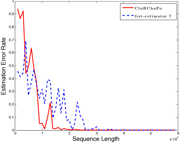
Figure 1: Average (over $40$ runs) error rates of our algorithm CluBChaPo$({\boldsymbol{x}},\lambda,r)$ and the list-estimator $\Upsilon$ of Khaleghi and Ryabko (2012a), as a function of the length $n$ of the input sequence ${\boldsymbol{x}}\in\mathbb{R}^{n}$, where ${\boldsymbol{x}}$ has $\kappa=4$ change-points $\lambda_{\min}:=0.1$ apart and is generated by $r=3$ distributions; $\lambda:=0.6\lambda_{\min}$. The error of $\Upsilon({\boldsymbol{x}},\lambda)$ is based on its first $\kappa$ elements.

The distributions and the procedure to generate a sequence ${\boldsymbol{x}}:=X_{1},\dots,X_{m}\in\mathbb{R}^{m},~{}m\in\mathbb{N}$ are as follows. Fix a parameter $\alpha\in(0,1)$ and two uniform distributions ${\mathcal{U}}_{1}$ and ${\mathcal{U}}_{2}$. Let $r_{0}$ be drawn randomly from $[0,1]$. For each $i=1..m$ obtain $r_{i}:=r_{i-1}+\alpha\mod 1$ and draw $x^{(j)}_{i}$ from ${\mathcal{U}}_{j},~{}j=1,2$. Finally set $X_{i}:=\mathbb{I}\{r_{i}\leq 0.5\}x_{i}^{(1)}+\mathbb{I}\{r_{i}>0.5\}x_{i}^{(2)}$. If $\alpha$ is irrational this produces a real-valued stationary ergodic time-series. In the experiments we fixed three parameters $\alpha_{1}:=0.12..,~{}\alpha_{2}:=0.13..$ and $\alpha_{3}:=0.14..$ (with long mantissae) to correspond to $r=3$ different process distributions. To produce ${\boldsymbol{x}}\in\mathbb{R}^{n}$ we randomly generated $\kappa:=5$ change-points $\theta_{k},~{}k=1..\kappa$ at least $\lambda_{\min}$ apart, with $\lambda_{\min}:=0.1$. Every segment of length $n_{k}:=n(\theta_{k}-\theta_{k-1}),~{}k=1..\kappa+1$ with $\theta_{0}:=0,~{}\theta_{\kappa+1}:=1$ was generated with $\alpha_{k^{\prime}}$ and $n_{k}$ where $k^{\prime}:=k\mod r,~{}k=0..\kappa+1$. In our experiments we provide $\lambda:=0.6\lambda_{\min}$ as input and calculate the error as $\mathbb{I}\{|\mathcal{C}|\neq\kappa\}+\mathbb{I}\{|{\mathcal{C}|=\kappa\}}\sum_{k=1}^{\kappa}|\hat{\theta}_{k}-\theta_{k}|$.

Note that, with this data generation procedure, the single-dimensional marginals are the same throughout the sequence. Most of the existing algorithms do not work at all in this scenario. To the best of our knowledge, the only work to address the change-point problem under this general framework is that of Khaleghi and Ryabko (2012a), which we use here for comparison. However, this method is a list-estimator in the sense of Definition 3 and makes no attempt to estimate $\kappa$. It simply generates a sorted list of estimates, whose first $\kappa$ elements converge to the true change-points; we calculate the error on the first $\kappa$ elements of its output.

7 Discussion

We have presented an asymptotically consistent method to estimate the number of change-points and do locate the changes in highly dependent time-series data. The considered framework is very general and as such is suitable for real-world applications.

Note that in this setting rates of convergence (even of frequencies to respective probabilities) are provably impossible to obtain. Therefore, unlike in the traditional settings for change-point analysis, the algorithms developed for this framework are forced not to rely on any rates of convergence. We see this as an advantage of the framework as it means that the algorithms are applicable to a much wider range of situations. At the same time, it may be interesting to derive the rates of convergence of the proposed algorithm under stronger assumptions (e.g., i.i.d.  data, or some mixing conditions). We conjecture that the algorithm is indeed optimal (up to some constant factors) in such settings as well (although it clearly cannot be optimal under parametric assumptions); however, we leave this as future work.

In the proposed algorithm a specific consistent clustering method is used to estimate the number of change-points. An interesting extension would be to establish the consistency of this method using any list-estimator in combination with any time-series clustering algorithm, that possess suitable asymptotic consistency guarantees.

Finally, the consistency of the algorithm is established when the distributional distance is used as the distance between the segments. The proof relies on some properties specific to this distance. Other distances can also be used in problems concerning stationary ergodic time series (e.g., Ryabko and Mary, 2012); thus, it is interesting to investigate which distances can be used with the algorithm proposed in the current paper.

References

- (1)
- Basseville and Nikiforov (1993) Basseville, M. and Nikiforov, I. (1993), Detection of abrupt changes: theory and application, Prentice Hall information and system sciences series, Prentice Hall.
- Brodsky and Darkhovsky (1993) Brodsky, B. and Darkhovsky, B. (1993), Nonparametric methods in change-point problems, Mathematics and its applications, Kluwer Academic Publishers.
- Carlstein and Lele (1993) Carlstein, E. and Lele, S. (1993), ‘Nonparametric change-point estimation for data from an ergodic sequence’, Teor. Veroyatnost. i Primenen. 38, 910–917.
- Giraitis et al. (1996) Giraitis, L., Leipus, R. and Surgailis, D. (1996), ‘The change-point problem for dependent observations’, Journal of Statistical Planning and Inference 53(3).
- Gray (1988) Gray, R. (1988), Prob. Random Processes, & Ergodic Properties, Springer Verlag.
- Hariz et al. (2007) Hariz, S. B., Wylie, J. and Zhang, Q. (2007), ‘Optimal rate of convergence for nonparametric change-point estimators for nonstationary sequences’, Annals of Statistics 35(4), 1802–1826.
- Khaleghi and Ryabko (2012a) Khaleghi, A. and Ryabko, D. (2012a), Locating changes in highly-dependent data with unknown number of change points, in ‘Neural Information Processing Systems (NIPS)’, Lake Tahoe, Nevada, United States.
- Khaleghi and Ryabko (2012b) Khaleghi, A. and Ryabko, D. (2012b), ‘Multiple change point estimation in stationary ergodic time series’, ArXiv e-print 1203.1515 .
- Khaleghi et al. (2012) Khaleghi, A., Ryabko, D., Mary, J. and Preux, P. (2012), Online clustering of processes, in ‘the international conference on Artificial Intelligence & Statistics (AI & Stats)’, La Palma, Canary Islands, pp. 601–609.
- Lavielle (2005) Lavielle, M. (2005), ‘Using penalized contrasts for the change-point problem’, Signal Processing 85(8), 1501 – 1510.
- Lebarbier (2005) Lebarbier, E. (2005), ‘Detecting multiple change-points in the mean of gaussian process by model selection’, Signal Processing 85(4), 717 – 736.
- Ryabko (2010a) Ryabko, D. (2010a), Clustering processes, in ‘the International Conference on Machine Learning (ICML)’, Haifa, Israel, pp. 919–926.
- Ryabko (2010b) Ryabko, D. (2010b), ‘Discrimination between B-processes is impossible’, Journal of Theoretical Probability 23(2), 565–575.
- Ryabko and Mary (2012) Ryabko, D. and Mary, J. (2012), Reducing statistical time-series problems to binary classification, in ‘Neural Information Processing Systems (NIPS)’, Lake Tahoe, Nevada, United States, pp. 2069–2077.
- Ryabko and Ryabko (2010) Ryabko, D. and Ryabko, B. (2010), ‘Nonparametric statistical inference for ergodic processes’, IEEE Transactions on Information Theory 56(3).
- Shields (1996) Shields, P. (1996), The Ergodic Theory of Discrete Sample Paths, AMS Bookstore.