Abstract: The paper starts out with a computational technique that allows to compare all linear methods for PDE solving that use the same input data. This is done by writing them as linear recovery formulas for solution values as linear combinations of the input data. Calculating the norm of these reproduction formulas on a fixed Sobolev space will then serve as a quality criterion that allows a fair comparison of all linear methods with the same inputs, including finite–element, finite–difference and meshless local Petrov–Galerkin techniques. A number of illustrative examples will be provided. As a byproduct, it turns out that a unique error–optimal method exists. It necessarily outperforms any other competing technique using the same data, e.g. those just mentioned, and it is necessarily meshless, if solutions are written “entirely in terms of nodes” (Belytschko et. al. 1996 [4]). On closer inspection, it turns out that it coincides with symmetric meshless collocation carried out with the kernel of the Hilbert space used for error evaluation, e.g. with the kernel of the Sobolev space used. This technique is around since at least 1998, but its optimality properties went unnoticed, so far.

1 Introduction

For simplicity, consider a standard Dirichlet problem

$$\begin{array}[]{rcll}Lu&=&f&\hbox{ in }\Omega\\ Bu&=&g&\hbox{ in }\Gamma:=\partial\Omega\\ \end{array}$$ (1)

with a linear differential operator $L$ and a linear boundary operator $B$ posed on a domain $\Omega$. Assume that the amount of available information is fixed and limited, namely to values

$$\begin{array}[]{rlll}f(x_{j})&\hbox{ in points }&x_{j}\in\overline{\Omega},&1\leq j\leq m,\\ g(y_{k})&\hbox{ in points }&y_{k}\in\Gamma:=\partial\Omega,&1\leq k\leq n.\\ \end{array}$$ (2)

Under all methods for solving such problems, we ask for the one with smallest error that uses this information and not more. To make this more precise, we fix a single point $x\in\overline{\Omega}$ and assume existence of a true solution $u^{*}$ of the problem. Any method $\mathcal{M}$ using the above information will produce some numerical solution $\tilde{u}_{\mathcal{M}}$, and we want to single out methods that make the error $|u^{*}(x)-\tilde{u}_{\mathcal{M}}(x)|$ small for all problems posed that way. We achieve this by looking at error bounds

$$|u^{*}(x)-\tilde{u}_{\mathcal{M}}(x)|\leq C_{\mathcal{M}}\|u^{*}\|_{H}\hbox{ for all }u^{*}\in H,$$

where the problems and their solutions are allowed to vary in such a way that the true solutions lie in some fixed reproducing kernel Hilbert space $H$ of functions on $\Omega$, e.g. a fixed Sobolev space. In this sense, the constant $C_{\mathcal{M}}$ describes the worst–case error behavior of the method $\mathcal{M}$ on all problems with solutions in $H$ using the same data. We shall show how to evaluate $C_{\mathcal{M}}$ numerically, and this will allow fair comparisons between methods using the same data. A few examples including important methods like finite elements, gerneralized finite differences, and meshless collocation in various forms are provided at the end.

But one can also ask for a method $\mathcal{M}$ that makes $C_{\mathcal{M}}$ minimal over all linear methods using the same data. This problem will be written as one of optimal recovery of functions, and it is proven that the optimal solution exists uniquely. It can be calculated explicitly, takes the form of a recovery method in reproducing kernel Hilbert spaces, and is a meshless method, if users ask for values of the solution at nodes. Since it is optimal in the above sense, it outperforms errorwise any other competing technique using the same data, may it use finite elements, finite differences, or local Petrov–Galerkin techniques. Upon closer inspection, it turns out to be nothing new, since it is a special case of symmetric meshless collocation, computed using the kernel that was used for error assessment. This method relies on Hermite–Birkhoff interpolation in reproducing kernel Hilbert spaces [20] and its application to PDE solving was first analyzed in [7, 8].

2 Recovery Problems

To keep the presentation simple, we stay with the Dirichlet problem example. Any linear method that provides an approximate solution value $\tilde{u}(x)$ for a fixed point $x$ and uses exclusively the data (2), must necessarily satisfy a formula of the form

$$\tilde{u}(x)=\displaystyle{\sum_{j=1}^{m}r_{j}(x)f(x_{j})+\sum_{k=1}^{n}s_{k}(x)g(y_{k}),}$$ (3)

whatever the weights $r_{j}(x)$ and $s_{k}(x)$ are. We call this a direct linear recovery of the value $\tilde{u}(x)$ from the data on the right–hand side. The existence of (3) follows from linearity and the restriction to the admitted data, but in general it will need some effort to rewrite a classical method in this form. We come back to this in the section on specific methods.

Clearly, the error in (3) is

$$u^{*}(x)-\tilde{u}(x)=u^{*}(x)-\displaystyle{\sum_{j=1}^{m}r_{j}(x)\Delta u^{*}(x_{j})-\sum_{k=1}^{n}s_{k}(x)u^{*}(y_{k})},$$

where we now have connected the data functions $f$ and $g$ back to the true solution $u^{*}$. The map

$$\epsilon_{x,\mathbf{r},\mathbf{s}}\;:\;u^{*}\mapsto u^{*}(x)-\displaystyle{\sum_{j=1}^{m}r_{j}(x)\Delta u^{*}(x_{j})-\sum_{k=1}^{n}s_{k}(x)u^{*}(y_{k})}$$ (4)

is a linear functional in $u^{*}$, and if it is bounded on some Hilbert space $H$, we have an error bound

$$|u^{*}(x)-\tilde{u}(x)|\leq\|\epsilon_{x,\mathbf{r},\mathbf{s}}\|_{H^{*}}\|u^{*}\|_{H}\hbox{ for all }u^{*}\in H.$$ (5)

If the norm $\|\epsilon_{x,\mathbf{r},\mathbf{s}}\|_{H^{*}}$ is evaluated, it precisely describes the worst–case error behavior for all problems with solutions in $H$, because the inequality is sharp by definition of the norm of the functional. In other words, one can express the error explicitly in percent of $\|u^{*}\|_{H}$, and this is what we shall do in the rest of the paper. Furthermore, one can ask for a choice $\mathbf{r}^{*}$ and $\mathbf{s}^{*}$ of the coefficients that make the norm minimal, and this will later lead to an optimal method for the given reconstruction.

Note that we do not consider the way numerical solutions of the considered methods are actually calculated. The amount of numerical integration needed for weak methods, the error committed in integration subroutines, and any multigrid solver techniques are completely irrelevant. Different numerical strategies within the same class of methods, e.g. finite element solvers with different ways of integration or with different element families can be compared directly as well. The only requirement is that the method is rewritten in direct linear recovery form (3), and then the total error is evaluated, containing all method–specific internal features of the technique.

3 Error Evaluation

Fortunately, it is easy to evaluate such norms in reproducing kernel Hilbert spaces, and Sobolev spaces are examples. In such spaces, the inner product and the kernel $K\;:\;\Omega\to\Omega$ have the properties

$$\begin{array}[]{rcl}f(x)&=&(f,K(x,\cdot))_{H}\hbox{ for all }f\in H,\;x\in\Omega\\ K(x,y)&=&(K(x,\cdot),K(y,\cdot))_{H}\hbox{ for all }x,y\in\Omega\\ \end{array}$$

and for all linear and continuous functionals $\lambda,\mu\in H^{*}$,

$$\begin{array}[]{rcl}(\lambda,\mu)_{H^{*}}&=&(\lambda^{x}K(x,\cdot),\mu^{y}K(y,\cdot))_{H}\\ &=&\lambda^{x}\mu^{y}K(x,y),\end{array}$$

where the upper index at the functionals denotes the variable that is acted upon. Details are in the literature on kernels, with [19] being a fairly complete reference and [15, 16] being open access compilations for teaching purposes.

Global Sobolev spaces $W_{2}^{m}(\mathbb{R}^{d})$ in $d$ dimensions and for order $m>d/2$ in the standard Fourier transform definition have the radial Matérn reproducing kernel

$$K(x,y)=\displaystyle{\frac{2^{1-m}}{\Gamma(m)}}\|x-y\|_{2}^{m-d/2}K_{m-d/2}(\|x-y\|_{2}),\;x,y\in\mathbb{R}^{d}$$ (6)

with the modified Bessel function $K_{m-d/2}$ of the second kind. Local Sobolev spaces $W_{2}^{m}(\Omega)$ for domains $\Omega\subset\mathbb{R}^{d}$ are norm–equivalent to the global spaces, as long as domains are non–pathological, i.e. they satisfy a Whitney extension property or a have a piecewise smooth boundary with a uniform interior cone condition. We shall use the above kernels for evaluation of errors in Sobolev space.

To avoid double sums and to pave the way for generalizations, we shall calculate the error norms after rewriting (4) in terms of functionals as

$$\epsilon_{x,\mathbf{c}}=\delta_{x}-\displaystyle{\sum_{k=1}^{N}c_{k}(x)\lambda_{k}}$$

with

$$\lambda_{j}(u)=Lu(x_{j}),\;1\leq j\leq m,\hbox{ and }\lambda_{m+i}(u)=u(y_{i}),\;1\leq i\leq n,\;N=m+n$$ (7)

in our special case. It should be clear that other differential operators and other boundary conditions will just change the functionals here.

Then we get the quadratic form

$$\begin{array}[]{rcl}\|\epsilon_{x,\mathbf{c}}\|^{2}_{H^{*}}&=&K(x,x)-2\displaystyle{\sum_{i=1}^{N}c_{i}(x)\lambda_{i}^{z}K(x,z)}\\ &&+\displaystyle{\sum_{j,i=1}^{N}c_{i}(x)c_{j}(x)\lambda_{i}^{y}\lambda_{j}^{z}K(y,z)}\end{array}$$ (8)

which can be explicitly evaluated if the kernel is known and the functionals are continuous, in particular on all Sobolev spaces on which the functionals are continuous. For instance, if $L$ is a second–order elliptic operator, this poses the restriction $m-2>d/2$ on the Sobolev order $m$ we can use. But this is normal, since we focus on methods that use $f=Lu^{*}$ pointwise, forcing $f$ to be in $W_{2}^{k}$ with $k>d/2$ and thus $u^{*}\in W_{2}^{m}$ with $m>2+d/2$. All methods that use these data are implicitly making this smoothness assumption, even if their users think that they are working in in less regular spaces. Plenty of papers and books miss this point. In particular, the standard FEM method is usually formulated and analyzed in low–regularity spaces like $H^{1}$ or $H^{2}$, but when it comes to implementations using data like (2), it needs $H^{m}$ with $m>3$ in $\mathbb{R}^{2}$.

All methods based on the data $\lambda_{1}(u^{*}),\ldots,\lambda_{K}(u^{*})$ and brought into the recovery form

$$\tilde{u}(x)=\displaystyle{\sum_{i=1}^{N}c_{i}(x)\lambda_{i}(u^{*})}$$

generalizing (2) and (4) can now be plugged into (8) to show how good the reproduction quality at $x$ is, since (5) generalizes accordingly. Note that there is no linear system to be solved once the recovery formula is known. But since the formula is inserted into the positive definite quadratic form (8), a small final value will necessarily contain quite some amount of cancellation. The computational complexity for norm evaluation is ${\cal O}(N^{2})$.

This allows a fair comparison of all such methods using the same data, and we shall provide examples below. The comparison can be made pointwise, as we saw, but for small problems one can plot the function $x\mapsto\|\epsilon_{x,\mathbf{c}}\|^{2}_{H^{*}}$ to see where a method works badly and needs more data. This gives direct information for refinement of the discretization.

4 Optimal Methods

Since (8) is a quadratic form with a positive semidefinite matrix, it can be minimized. The optimal solution coefficients $c_{i}^{*}(x)$ solve the system

$${\sum_{k=1}^{N}c_{k}^{*}(x)\lambda_{j}^{y}\lambda_{k}^{z}K(y,z)=\lambda_{j}^{z}K(x,z),\;1\leq j\leq N,}$$ (9)

and the system can be proven to be solvable [20]. Clearly, this choice of coefficients will then outperform all other competitors error–wise. We shall show examples later. The minimal value of (8) then is

$$\begin{array}[]{rcl}\|\epsilon_{x,\mathbf{c}^{*}}\|^{2}_{H^{*}}&=&K(x,x)-\displaystyle{\sum_{i=1}^{N}c_{i}(x)^{*}\lambda_{i}^{z}K(x,z)}\geq 0\end{array}$$

and does not contain any matrix.

The system (9) reveals the nature of this method. Indeed, the functions $c_{k}$ are necessarily linear combinations of the functions $\lambda_{i}^{z}K(\cdot,z)$, and application of $\lambda_{i}^{x}$ to the above system shows the Lagrange property $\lambda_{i}(c_{k})=\delta_{ik},\;1\leq i,k\leq N$. This means that the $c_{k}$ are the Lagrange basis for general Hermite–Birkhoff interpolation of the given data by the functions $\lambda_{i}^{z}K(\cdot,z)$,,and this is the well–known method of symmetric meshless collocation based on [20] and analyzed thoroughly in [8, 7]. The optimality of the technique in the sense of this paper should have been known since at least since 1997, but it went unnoticed because [15, p.82, (4.2.2)] was not applied to PDE solving at that time.

5 Special Methods

We now give some details on how to evaluate recovery errors for special PDE solution techniques. This will be useful for the examples in the final section, and we specialize to $L=-\Delta$ here.

5.1 Finite Elements

The simplest possible 2D finite–element code uses piecewise linear elements on the triangles of a triangulation of a domain with piecewise linear boundary, and requires $f$–values only at the barycenters of the triangles. These are the points $x_{j}$ in (2) in the FEM version that we denote by FEMBary below. But since usually there are more triangles than nodes, one can also prescribe $f$–values at all interior and boundary nodes to calculate approximate values at the barycenters. This usually needs less $f$–values at the same order of accuracy. We call this method FEMNode below. These two FEM variations have different recovery formulas (3) and different error functionals (4) to be compared.

To get the recovery formulas in the form needed here, users will have to check carefully what their FEM code does. We used the MATLAB pdetool setting, which does the following. It uses all $N$ triangle vertices $z_{1},\ldots,z_{N}$ for setting up the standard piecewiese linear test and trial functions $v_{1}.\ldots,v_{N}$ with $v_{j}(z_{k})=\delta_{jk}$ and builds the $N\times N$ stiffness matrix with entries $(\nabla v_{i},\nabla v_{j})_{L_{2}}$ in the usual way. The right–hand sides $(f,v_{j})_{L_{2}},\;1\leq j\leq N$ are certain linear combinations of $f$–values either at triangle barycenters or at nodes of the neighboring triangles. These linear combinations form a sparse integration matrix $\mathbf{B}$ with entries $b_{jk}$ such that the stiffness system without boundary conditions but with some form of numerical integration would be

$${\sum_{i=1}^{N}(\nabla v_{i},\nabla v_{j})_{L_{2}}u(z_{i})=\sum_{k=1}^{N}b_{jk}f(x_{k}),\;1\leq j\leq N.}$$

The FEMBary and FEMNode variations have different $\mathbf{B}$ matrices and use $f$ at different points $x_{k}$, but the stiffness matrices are the same.

The unknowns $u(z_{i}),\;i\in D\subset\{1,\ldots,N\}$ are known Dirichlet values, and thus

$${\sum_{i\notin D}(\nabla v_{i},\nabla v_{j})_{L_{2}}u(z_{i})=\sum_{k=1}^{N}b_{jk}f(x_{k})-\sum_{i\in D}(\nabla v_{i},\nabla v_{j})_{L_{2}}u(z_{i}),\;j\notin D}$$

is the system to be actually solved. Since the $u(z_{i})$ with $i\in D$ are $g$–values, it has the matrix–vector form

$$\mathbf{A}\mathbf{u}=\mathbf{B}\mathbf{f}+\mathbf{C}\mathbf{g}$$ (10)

under adequate notation, and each row of

$$\mathbf{u}=\mathbf{A}^{-1}\mathbf{B}\mathbf{f}+\mathbf{A}^{-1}\mathbf{C}\mathbf{g}$$

provides one instance of (3) for each of the points $x=x_{i},\;i\notin D$. If we focus on the origin as one of these points, we need just one row.

If users want the error at a non–nodal point $x$, they have to add a piecewise linear interpolation on a triangle containing $x$, and then the discrete reconstruction formula is a linear combination of three rows of the above system. This illustrates how numerical integration and interpolatory post–processing both enter explicitly into our version of a complete and explicit FEM error analysis.

5.2 Symmetric Kernel–Based Collocation

These work on the two point sets $X$ and $Y$ from (2) and use linear combinations

$$u(x)=\displaystyle{\sum_{j=1}^{m}c_{j}\Delta K(x,x_{j})+\sum_{k=1}^{n}d_{k}K(x,y_{k})}$$ (11)

of basis functions derived from a smooth kernel $K$. The argument in Section 4 shows that these methods yield optimal errors in the Hilbert spaces in which their kernels are reproducing. In case of Sobolev spaces, we thus get the error–optimal methods this way.

The numerical process collocates these trial functions at Dirichlet and PDE nodes, forming the block system

$$\begin{array}[]{rcl}\displaystyle{\sum_{j=1}^{m}c_{j}\Delta^{x}\Delta^{y}K(x_{i},x_{j})+\sum_{k=1}^{n}d_{k}\Delta K(x_{i},y_{k})}&=&f(x_{i}),\;1\leq i\leq m,\\ \displaystyle{\sum_{j=1}^{m}c_{j}\Delta K(y_{i},x_{j})+\sum_{k=1}^{n}d_{k}K(y_{i},y_{k})}&=&g(y_{i}),\;1\leq i\leq n.\end{array}$$

The inverse of the coefficient matrix recovers the coefficients $c_{j}$ and $d_{k}$ from the $f$ and $g$ data, and the numerical solution at $x$ is just a linear combination (11) of those coefficients. Consequently, the discrete recovery (3) is furnished by the inverse of the above “stiffness” matrix, premultiplied by the row vector of the kernel values in (11).

Of course. one can use a special kernel $K$ to calculate the discrete recovery, and then use another kernel, e.g. one generating a Sobolev space, for error evaluation on that space. We shall do this in the final section.

5.3 Unsymmetric Kernel–Based Collocation

In contrast to the previous section, this class of methods takes an additional set $Z=\{z_{1},\ldots,z_{N}\}$ of usually $N=m+n$ points and works on linear combinations

$$u(x)=\displaystyle{\sum_{k=1}^{N}d_{k}K(x,z_{k})}$$ (12)

of basis functions, while still using collocation in the point sets $X$ and $Y$ from (2). This method dates back to early papers of Ed Kansa [10, 11] and was called MLSQ2 as a variation of the Meshless Local Petrov–Galerkin method [2, 1] of S.N. Atluri and collaborators. The linear system for the coefficients now is

$$\begin{array}[]{rcl}\displaystyle{\sum_{k=1}^{n}d_{k}\Delta K(x_{i},z_{k})}&=&f(x_{i}),\;1\leq i\leq m,\\ \displaystyle{\sum_{k=1}^{n}d_{k}K(y_{i},z_{k})}&=&g(y_{i}),\;1\leq i\leq n,\end{array}$$

and the inverse of the coefficient matrix (if it exists, see [9]), premultiplied by the vector of values $K(x,z_{k})$ of (12) will yield a row vector for the discrete recovery formula (3). If $N$ is chosen larger than $m+n$ to increase stability, a pseudoinverse of the system coefficient matrix can replace the inverse. This was done in the examples of the final section.

5.4 Meshless Lagrange Methods

Here, a set $Z=\{z_{1},\ldots,z_{N}\}$ of trial nodes is chosen, and there are shape functions $u_{1},\ldots,u_{N}$ such that trial functions

$$u(x)=\displaystyle{\sum_{k=1}^{N}u_{k}(x)u(z_{k})}$$

can be written “entirely in terms of nodes”. Usually, this implies Lagrange conditions $u_{j}(z_{k})=\delta_{jk}$, and in many cases the shape functions are defined via Moving Least Squares. We do not care here for details, and allow such techniques to come in weak or strong form. The strong case collocates in sets $X$ and $Y$ like above, forming a system

$$\begin{array}[]{rcl}\displaystyle{\sum_{k=1}^{N}\Delta u_{k}(x_{j})u(z_{k})}&=&f(x_{j}),\;1\leq j\leq m,\\ \displaystyle{\sum_{k=1}^{N}u_{k}(y_{i})u(z_{k})}&=&g(y_{i}),\;1\leq i\leq n\\ \end{array}$$

and the weights of the discrete recovery at $z_{k}$ will be a row of the preudoinverse of the coefficient matrix of this system.

The weak cases form stiffness matrices and right–hand sides like in the FEM situation, and then we get the coefficients of the discrete recovery in the same way, involving a special matrix $\mathbf{B}$ caring for the numerical integration.

5.5 Generalized Finite–Difference Methods

Here, there are no trial functions, but everything is still expressed in terms of values at nodes $Z=\{z_{1},\ldots,z_{N}\}$. In the strong situation, PDE operator values are approximated by formulas like

$$\Delta u(x_{j})\approx\displaystyle{\sum_{i=1}^{N}\alpha_{jk}u(z_{k}),}$$ (13)

with localized weights $\alpha_{jk}$, and this can be done with minimal error in a reproducing kernel Hilbert space using the logic of section 4. See [6, 17] for more details. The linear system then is

$$\begin{array}[]{rcl}f(x_{j})&=&\displaystyle{\sum_{i=1}^{N}\alpha_{jk}u(z_{k}),}\\ f(x_{j})-\displaystyle{\sum_{i\in D}\alpha_{jk}u(z_{k}),}&=&\displaystyle{\sum_{i\notin D}\alpha_{jk}u(z_{k}),}\\ \end{array}$$

if we use a subset $D$ of Dirichlet nodes like in the FEM case. This is of the form (10) and we already know how to derive the recovery formulas in such a case. It is interesting to see that the matrix with coefficients $\alpha_{jk}$ plays the role of a stiffness matrix here, and it is the place where sparsity can be implemented to yield local methods with sparse matrices. This was very successfully done in various application papers of C.S. Chen, B. Sarler, and G.M. Yao [14, 22, 21, 23, 18]. We shall present a simple numerical example in the final section.

The Direct Meshless Local Petrov Galerkin methods of [12, 13] are weak cases of this approach, with other functionals than (13) being directly approximated in terms of values at nodes, and with integrations involving $\mathbf{B}$ matrices again, like in all other weak methods. We leave this for a future paper dealing with all variants of Atluri’s Meshless Local Petrov Galerkin technique, and comparing them to FEM and kernel methods, optimal or not, sparse or not.

6 Numerical Examples

To avoid overloading the paper, we present a simple series of examples. They all work on the unit circle for simplicity, and in order to include finite elements, we have to use triangulations, even if they are not needed for meshless methods. We start with the standard discretization of the unit circle into 8 triangles meeting at the origin, followed by three standard finite–element refinement steps halving the edges. The problem (1) is posed with $L=-\Delta$, and Dirichlet boundary values are always provided in the boundary nodes, which are the $y_{k}$ in (2). In all cases, the non–boundary vertices of the triangles are the nodes where we want to know the solution, but in the sense of (4) and for simplicity we only evaluate the recovery error at the origin $x=0$.

As the FEM variations show, one can work with $f$ values either in barycenters of triangles or in vertices of the triangulation. We shall evaluate all examples in both situations, denoting the methods by either *Bary or *Node. Details on the discretizations are in Table 1:

• $n$: number of Dirichlet boundary data points for $g$ values,

• $m_{Bary}$: number of triangles and barycentric data points for $f$ values,

• $m_{Node}$: number of vertices and vertex data points for $f$ values, including the $n$ Dirichlet boundary vertices,

• DOF: degrees of freedom $=$ number of unknowns $=m_{Node}-n$,

• $h$: fill distance in the sense of kernel discretizations, describing the maximal distance of an arbitrary point of the domain to one of the vertices.

Case	$n$	$m_{Bary}$	$m_{Node}$	DOF	$h$
C0	8	8	9	1	0.2706
C1	16	32	25	9	0.1515
C2	32	128	81	49	0.0768
C3	64	512	289	225	0.0389
C4	128	2048	1089	961	0.0197

Table 1: Discretization data for the examples on the unit disk

The plots in Figures 1 to 5 show the errors in Sobolev space of order 3 to 7, with order 3 being somewhat out of bounds, and the data for the fine discretization C4 being polluted by ill–conditioning in various cases. In each figure, the Sobolev space for error evaluation is fixed, but the methods might use other kernels. The methods are

• FEMBary: FEM with $f$ data in barycenters

• FEMNode: FEM with $f$ data in nodes

• KansaBary: Unsymmetric collocation with $f$ data in barycenters, using the order 7 Sobolev kernel

• KansaNode: same with node data

• HOBary: symmetric high-order collocation with $f$ data in barycenters, using the order 7 Sobolev kernel

• HONode: same with data in nodes. These two coincide with the optimal methods, if evaluated on Sobolev space of order 7, see Figure 5.

• OptBary: optimal method in Sobolev space used for error evaluation, with $f$ data in barycenters

• OptNode: same with data in nodes

• LocNode: a bandwidth 15 method like in section 5.5, using the order 7 Sobolev kernel, data in nodes.

There are serious instabilities that need explanation. They could have been avoided in all cases by choosing a smaller kernel scale, but this would have changed the Sobolev space norm and concealed the instabilities. Consequently, the kernel scale for Sobolev space error evaluation was fixed at 1.0 throughout. This does not seriously affect the error evaluation, because the latter just consists of a calculation of a quadratic form.

But it affects the calculation of recovery formulas by kernel methods, including the optimal ones. In particular, increasing the smoothness of the construction kernel will increase the instability, if no precautions like preconditioning [3, 5] are taken. We chose the Kansa* and the HO* kernel methods to work with the kernel of Sobolev space of order 7 at scale 1, but smaller scales would have been more stable. Users can easily try different kernels and scales for construction and then evaluate in a fixed Sobolev space at a fixed scale to see which construction scale gives best results. Example is missing

The numerical results support quantitatively what is known from experience and partly supported by theory. The piecewise linear FEM technique is adapted to low–regularity problems, and it shows its second–order convergence in all applicable Sobolev spaces from order 4 on. It is clearly inferior error–wise to the error–optimal method, which is symmetric collocation in Sobolev space, and the difference gets larger for increasing Sobolev order, because the optimal method behaves like a $p$–FEM and increases its convergence rate automatically with the Sobolev order. Unfortunately, it suffers from severe ill–conditioning if no precautions are taken, and it does not allow sparsity. However, it serves as a standard reference to evaluate error performances of all other methods using the same data.

We now list some observations concerning comparisons. The optimal method HO* for a fixed high Sobolev order performs well also for lower Sobolev order. It adapts automatically to lower regularity. Other competing methods, like Kansa* for unsymmetric collocation, behave in the same way. If sparsity is enforced by localizing meshless collocation [14, 22, 21, 23, 18], one gets competitive methods Loc* that share sparsity with FEM techniques, but also yield high convergence orders depending on the bandwidth chosen.

7 Conclusion and Outlook

The paper provides a tool that allows an explicit and fully computational assessment of the error behavior of all linear solvers for all linear PDE problems. The exact solution can be unknown, and the error is expressed as a factor of the (unknown) Sobolev norm of the true solution. This tool should be applied in many more circumstances, e.g. on special and awkward domains, for more general differential operators including those of Computational Mechanics, and for many other linear solvers, e.g. MLPG methods and boundary–oriented techniques like the DRM. Any application–oriented paper can, in principle, apply this technique and thus provide a strict worst–case error bound in terms of the Sobolev norm of the true solution. Examples of single cases with known solutions can never be completely satisfactory, but they are the usual practice in application papers.

There is a method that always realizes the optimal error, but it needs further work towards numerical stabilization. All other methods should be compared to it, and it is an interesting research challenge to see how close one can come to the optimal method under sparsity restrictions.

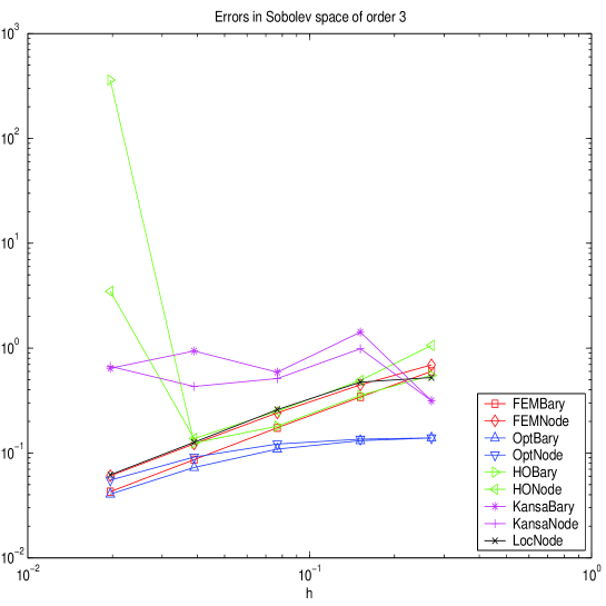
Figure 1: Errors for Sobolev order 3

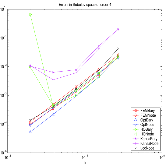
Figure 2: Errors for Sobolev order 4

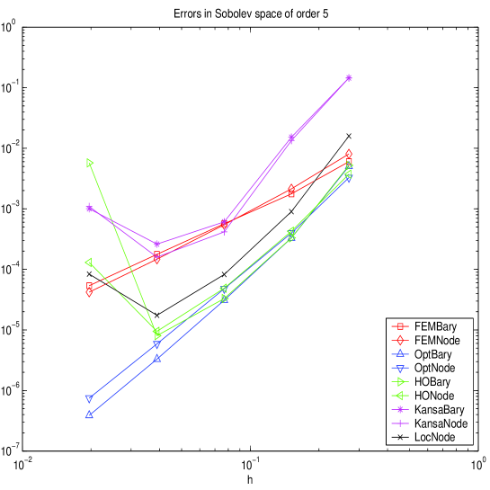
Figure 3: Errors for Sobolev order 5

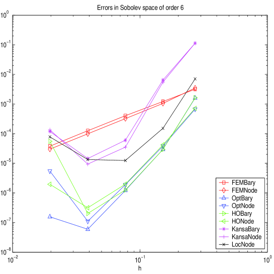
Figure 4: Errors for Sobolev order 6

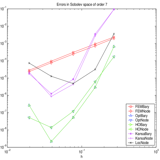
Figure 5: Errors for Sobolev order 7

	C0	C1	C2	C3	C4
h	2.706e-001	1.515e-001	7.682e-002	3.895e-002	1.965e-002
FEMBary	6.011e-001	3.415e-001	1.737e-001	8.635e-002	4.272e-002
FEMNode	6.912e-001	4.457e-001	2.411e-001	1.220e-001	6.063e-002
KansaBary	3.150e-001	1.422e+000	5.888e-001	9.385e-001	6.421e-001
KansaNode	3.150e-001	9.847e-001	5.131e-001	4.303e-001	6.696e-001
HOBary	5.510e-001	3.538e-001	1.802e-001	1.245e-001	3.605e+002
HONode	1.060e+000	4.918e-001	2.498e-001	1.371e-001	3.475e+000
OptBary	1.390e-001	1.309e-001	1.090e-001	7.280e-002	4.051e-002
OptNode	1.391e-001	1.353e-001	1.218e-001	9.145e-002	5.508e-002
LocNode	5.236e-001	4.734e-001	2.591e-001	1.264e-001	6.196e-002

Table 2: Raw data for Sobolev order 3

	C0	C1	C2	C3	C4
h	2.706e-001	1.515e-001	7.682e-002	3.895e-002	1.965e-002
FEMBary	2.223e-002	5.296e-003	1.301e-003	3.494e-004	9.856e-005
FEMNode	2.547e-002	7.813e-003	1.984e-003	4.844e-004	1.199e-004
KansaBary	1.995e-001	5.219e-002	7.806e-003	6.309e-003	1.049e-002
KansaNode	1.995e-001	4.215e-002	6.083e-003	3.478e-003	1.101e-002
HOBary	2.173e-002	4.353e-003	9.958e-004	4.171e-004	6.565e-001
HONode	2.446e-002	5.855e-003	1.479e-003	4.436e-004	9.688e-003
OptBary	2.163e-002	4.308e-003	9.355e-004	2.174e-004	5.287e-005
OptNode	2.029e-002	5.770e-003	1.463e-003	3.653e-004	9.117e-005
LocNode	4.265e-002	7.420e-003	1.651e-003	4.069e-004	1.364e-004

Table 3: Raw data for Sobolev order 4

	C0	C1	C2	C3	C4
h	2.706e-001	1.515e-001	7.682e-002	3.895e-002	1.965e-002
FEMBary	6.010e-003	1.762e-003	5.658e-004	1.775e-004	5.376e-005
FEMNode	8.042e-003	2.134e-003	5.451e-004	1.477e-004	4.202e-005
KansaBary	1.447e-001	1.522e-002	6.089e-004	2.612e-004	1.005e-003
KansaNode	1.447e-001	1.345e-002	4.163e-004	1.590e-004	1.092e-003
HOBary	5.223e-003	3.307e-004	3.299e-005	8.055e-006	5.733e-003
HONode	3.723e-003	4.258e-004	4.881e-005	9.465e-006	1.303e-004
OptBary	5.031e-003	3.304e-004	3.106e-005	3.298e-006	3.873e-007
OptNode	3.278e-003	3.977e-004	4.798e-005	5.890e-006	7.463e-007
LocNode	1.591e-002	8.987e-004	8.243e-005	1.742e-005	8.366e-005

Table 4: Raw data for Sobolev order 5

	C0	C1	C2	C3	C4
h	2.706e-001	1.515e-001	7.682e-002	3.895e-002	1.965e-002
FEMBary	3.167e-003	1.219e-003	4.051e-004	1.262e-004	3.780e-005
FEMNode	3.485e-003	1.054e-003	3.226e-004	9.917e-005	3.003e-005
KansaBary	1.135e-001	6.470e-003	6.036e-005	1.451e-005	1.186e-004
KansaNode	1.135e-001	5.501e-003	3.513e-005	9.405e-006	1.349e-004
HOBary	1.641e-003	2.955e-005	1.262e-006	2.034e-007	5.496e-005
HONode	7.159e-004	4.206e-005	1.983e-006	3.158e-007	1.965e-006
OptBary	1.600e-003	2.949e-005	1.222e-006	5.964e-008	1.566e-007
OptNode	6.730e-004	3.811e-005	1.901e-006	1.110e-007	5.458e-006
LocNode	7.056e-003	1.521e-004	1.247e-005	1.342e-005	7.800e-005

Table 5: Raw data for Sobolev order 6

	C0	C1	C2	C3	C4
h	2.706e-001	1.515e-001	7.682e-002	3.895e-002	1.965e-002
FEMBary	2.337e-003	9.327e-004	3.075e-004	9.490e-005	2.820e-005
FEMNode	1.975e-003	7.244e-004	2.425e-004	7.684e-005	2.339e-005
KansaBary	9.332e-002	3.506e-003	8.576e-006	1.232e-006	1.792e-005
KansaNode	9.332e-002	2.743e-003	4.428e-006	8.672e-007	2.207e-005
HOBary	6.633e-004	2.916e-006	5.232e-008	2.147e-009	2.658e-007
HONode	1.722e-004	6.116e-006	1.202e-007	1.390e-008	5.223e-008
OptBary	6.633e-004	2.916e-006	5.232e-008	2.147e-009	2.658e-007
OptNode	1.722e-004	6.116e-006	1.202e-007	1.390e-008	5.224e-008
LocNode	3.590e-003	3.179e-005	4.802e-006	1.273e-005	7.360e-005

Table 6: Raw data for Sobolev order 7

References

- [1] S. N. Atluri. The meshless method (MLPG) for domain and BIE discretizations. Tech Science Press, Encino, CA, 2005.
- [2] S. N. Atluri and T.-L. Zhu. A new meshless local Petrov-Galerkin (MLPG) approach in Computational Mechanics. Computational Mechanics, 22:117–127, 1998.
- [3] R.K. Beatson, J.B. Cherrie, and C.T. Mouat. Fast fitting of radial basis functions: Methods based on preconditioned GMRES iteration. Advances in Computational Mathematics, 11:253–270, 1999.
- [4] T. Belytschko, Y. Krongauz, D.J. Organ, M. Fleming, and P. Krysl. Meshless methods: an overview and recent developments. Computer Methods in Applied Mechanics and Engineering, special issue, 139:3–47, 1996.
- [5] D. Brown, L. Ling, E.J. Kansa, and J. Levesley. On approximate cardinal preconditioning methods for solving PDEs with radial basis functions. Engineering Analysis with Boundary Elements, 19:343–353, 2005.
- [6] O. Davydov and R. Schaback. Error bounds for kernel-based numerical differentiation. Draft, 2012.
- [7] C. Franke and R. Schaback. Convergence order estimates of meshless collocation methods using radial basis functions. Advances in Computational Mathematics, 8:381–399, 1998.
- [8] C. Franke and R. Schaback. Solving partial differential equations by collocation using radial basis functions. Appl. Math. Comp., 93:73–82, 1998.
- [9] Y.C. Hon and R. Schaback. On unsymmetric collocation by radial basis functions. J. Appl. Math. Comp., 119:177–186, 2001.
- [10] E. J. Kansa. Application of Hardy’s multiquadric interpolation to hydrodynamics. In Proc. 1986 Simul. Conf., Vol. 4, pages 111–117, 1986.
- [11] E. J. Kansa. Multiquadrics - a scattered data approximation scheme with applications to computational fluid-dynamics - I: Surface approximation and partial dervative estimates. Comput. Math. Appl., 19:127–145, 1990.
- [12] D. Mirzaei and R. Schaback. Direct Meshless Local Petrov-Galerkin (DMLPG) method: A generalized MLS approximation. Preprint Göttingen, 2011.
- [13] D. Mirzaei, R. Schaback, and M. Dehghan. On generalized moving least squares and diffuse derivatives. IMA J. Numer. Anal., 32, No. 3:983–1000, 2012. doi: 10.1093/imanum/drr030.
- [14] Božidar Šarler. From global to local radial basis function collocation method for transport phenomena. In Advances in meshfree techniques, volume 5 of Comput. Methods Appl. Sci., pages 257–282. Springer, Dordrecht, 2007.
- [15] R. Schaback. Reconstruction of multivariate functions from scattered data. Manuscript, available via http://www.num.math.uni-goettingen.de/schaback/research/group.html, 1997.
- [16] R. Schaback. Kernel–based meshless methods. Lecture Note, Göttingen, 2011.
- [17] R. Schaback. Direct discretizations with applications to meshless methods for PDEs. submitted, http://www.num.math.uni-goettingen.de/schaback/research/group.html, 2013.
- [18] Robert Vertnik and Božidar Šarler. Local collocation approach for solving turbulent combined forced and natural convection problems. Adv. Appl. Math. Mech., 3(3):259–279, 2011.
- [19] H. Wendland. Scattered Data Approximation. Cambridge University Press, 2005.
- [20] Z. Wu. Convergence of interpolation by radial basis functions. Chinese Ann. Math. Ser. A, 14:480–486, 1993.
- [21] Guangming Yao, Bozidar Šarler, and C. S. Chen. A comparison of three explicit local meshless methods using radial basis functions. Eng. Anal. Bound. Elem., 35(3):600–609, 2011.
- [22] Guangming Yao, Siraj ul Islam, and Božidar Šarler. A comparative study of global and local meshless methods for diffusion-reaction equation. CMES Comput. Model. Eng. Sci., 59(2):127–154, 2010.
- [23] Guangming Yao, Siraj ul Islam, and Božidar Šarler. Assessment of global and local meshless methods based on collocation with radial basis functions for parabolic partial differential equations in three dimensions. Eng. Anal. Bound. Elem., 36(11):1640–1648, 2012.