HARTREE–FOCK PROBLEM OF AN ELECTRON-HOLE PAIR IN THE QUANTUM WELL GaN

Abstract

We present microscopic calculations of the absorption spectra for $\textrm{GaN}/\textrm{Al}_{x}\textrm{Ga}_{1-x}\textrm{N}$ quantum well systems. Whereas the quantum well structures with the parabolic law of dispersion exhibit the usual bleaching of an exciton resonance without shifting a spectral position, the significant red-shift of an exciton peak is found with increasing the electron-hole gas density for a wurtzite quantum well. The energy of the exciton resonance for a wurtzite quantum well is found. The obtained results can be explained by the influence of the valence band structure on quantum confinement effects. The optical gain spectrum in the Hartree–Fock approximation and the Sommerfeld enhancement are calculated. A red shift of the gain spectrum in the Hartree–Fock approximation with respect to the Hartree gain spectrum is found.

1 Introduction

The physical properties of wide bandgap group-III quantum well systems are under investigation due to their application to light emitters and semiconductor lasers in the ultraviolet, blue, and green wavelength regions. Ultraviolet light-emitting diodes and lasers have recently obtained considerations due to applications to the compact biological detection systems, analytical devices, and medical diagnostics. A number of light-emitting diodes and laser diodes have been demonstrated [1,​ 2]. However, these structures are in the developmental stage, and there are many questions with respect to the performance and device configurations.

Realizing the deep-ultraviolet semiconductor-based light-emitting diodes provides light sources for various applications, for instance to the biological detection and the data storage. Although such devices basically need a $\textrm{Al}_{x}\textrm{Ga}_{1-x}\textrm{N}$-based quantum well with high Al contents, their fundamental optical properties remain under discussion. It has been proved experimentally that the surface emission from [0001]-oriented $\textrm{Al}_{x}\textrm{Ga}_{1-x}\textrm{N}$ is quite weak because of the predominant optical polarization along the [0001] $c$ direction [3,​ 4,​ 5]. The explanation of these effects may be found from the difference of structures of the valence bands in AlN and in GaN. In wurtzite GaN or AlN, the degeneracy of the $p$-like states at the $\Gamma$ point is lifted by both crystal-field splitting and spin-orbit splitting leading to forming three valence bands at the Brillouin zone center.

Since AlN has a negative crystal field splitting energy, while GaN has a positive one, these splittings lead to the ordering of the valence band in AlN: $\Gamma_{7}$, $\Gamma_{9},$ and $\Gamma_{7}.$ Whereas we have $\Gamma_{9}$, $\Gamma_{7},$ and $\Gamma_{7}$ in GaN [6]. Therefore, the topmost of the valence band in AlN has the crystal field split off holes with $p_{z}$-states, while the topmost in GaN has the heavy holes with $p_{x}$-like and $p_{y}$-like states, where the axis $z$ is directed along the hexagonal axis.

Therefore, the emission from $\textrm{Al}_{x}\textrm{Ga}_{1-x}\textrm{N}$ with high (low) Al-content is polarized along (perpendicular to) the $c$ axis.

Recently, many studies have been focused on the potential application of nanostructures, such as photonic crystal structures, nanoholes, nanodots, and nanorods. In the studies of the technology involving the photonic band gap, it seems that, in the case of dielectric rod nanoarrays or nanocolumns, a large gap is opened for the TM mode, but not for the TE one [7]. Thus, with this type of structures for laser applications, the light source in the TM mode is obtained.

In the $c$-plane of InGaN/GaN quantum well systems, the compressive strain is induced in the active layer, and the light is TE-polarized [8]. Furthemore, there is a strong internal electric field caused by the spontaneous and piezoelectric polarization charges at the interfaces of the $c$-plane of the InGaN/GaN quantum well. This phenomenon leads to the quantum confined Stark effect, decreases the internal quantum efficiency, and leads to the emission spectrum which is red-shifted.

In some studies [9,​ 10,​ 11] of interface polarization charges, alloy materials were used to make a better performance. Many works have focused on the nonpolar and semipolar planes [12,​ 13,​ 14,​ 15]. These results have testified that the light emission will be polarized, and the quantum confined Stark effect will be reduced. However, due to a higher cost of the $a$- and $m$-plane substrates, it would be better to use the $c$-plane substrate. In work  [16,​ 17], the $c$-plane of the InGaN/AlGaN quantum well structure was considered instead of that of InGaN/GaN in order to obtain a tensile strain in the quantum well layer. The previous studies and calculations have shown that the $|Z\rangle$-like state is generated in nitride materials, if the quantum well layer is under a tensile biaxial strain.

Besides the nitride-based devices, the group-II oxides have been considered for highly efficient laser diodes [18,​ 19] and high-performance field-effect transistors [21,​ 22]. The induced piezoelectric field plays a significant role for both band structure and optical gain [23]. However, the orientation of a crystal structure significantly modifies the band structure through the strain effect  [24]. It has been proved experimentally that the growth along crystal directions different from the [0001] direction leads to an increase in the quantum efficiency by decreasing the strain-induced electric field in the quantum well region, possibly leading to the ways of obtaining highly efficient white laser diodes [25]. There are the theoretical works studying the effects of crystal orientation on the piezoelectric field in a strained wurtzite quantum well [24,​ 26]. However, the piezoelectric effect consists not only of a strain-induced polarization; it also takes the response of both electric field and polarization on the strain into consideration. These effects were studied in paper [26].

A deeper understanding of the influence of band structures on optical properties should help one to answer many questions. In addition, the interesting effects of strong electron-hole Coulomb interaction are presented in these materials. Many-body interactions lead to effects, which consist the screening, dephasing, bandgap renormalization, and phase-space filling [27,​ 28,​ 29,​ 30].

A general phenomenon of Coulomb enhancement may be explained as follows. Due to the Coulomb attraction, an electron and a hole have a larger tendency to be located near each other, than that in the case of noninteracting particles. This increase of the interaction duration leads to an increase of the optical transition probability.

The paper is organized as follows. In Section 2, we present the microscopic many-body theory, which is based on the Bloch equations for semiconductors, i.e., the Heisenberg equations for the optical polarization and the populations of carriers. In Section 3, we consider a quantum well, which is oriented perpendicularly to the growth direction [0001]. We research the overlap integral of electron and hole wave functions and calculate the exciton binding energy in the quantum well. We calculate the Hartree and Hartree–Fock gain spectra. We calculate the exciton absorption spectra in the wurtzite quantum well and compare them with the absorption spectra in a quantum well with parabolic bands. We calculate the Hartree and Hartree–Fock renormalization energy spectra and the red shift of the gain spectra caused by an electron-electron and hole-hole Coulomb interaction. A significant Sommerfeld enhancement of the spectrum is determined. This enhancement of the electric dipole moment caused by the electron-hole Coulomb attraction.

2 Theory

Let us consider the points of zero slope, i.e., the points at which the speed components $\frac{\partial\,E}{\partial\,k_{\alpha}}$ are identically equal zero according to the symmetry conditions taking into account the time inversion invariance. These points are determined by the formula $N=\frac{1}{h^{\prime}}\sum_{g\in\,G}\frac{1}{2}[\chi_{v}^{2}(g)+\chi_{v}(g^{2})]\frac{1}{2}[\chi_{\psi}^{2}(g)+\chi_{\psi}(g^{2})]$. In this case, all momentum components become zero, i.e., $\frac{\partial\,E}{\partial\,k_{\alpha}}=0$ for an all directions k [31].

We consider a quantum well, which is oriented perpendicularly to the growth direction [0001]. The axis $z$ is directed along the hexagonal $c$ axis. Then a longitudinal wave vector $k_{z}$ is changed by the operator $k_{z}\rightarrow\,-i\frac{\partial}{\partial\,z}$. From the Schrödinger equation, we obtain the energy spectrum $E_{n}(k_{t})$ for holes and for electrons, where $k_{t}=(k_{x},k_{y})$ is a transversal wave vector. The necessary condition of a band extremum in a vicinity of the band gap is the zero derivative of the energy with respect to $k_{t}$. It is known from semiconductor physics that the absorption spectrum in a vicinity of the band gap with regard for a coupled electron-hole pair leads to an exciton spectrum. The excitons mathematically obey the Schrödinger equation for a hydrogen atom, which is known as the Wannier equation [32].

The complete orthonormal system of functions for holes depends on three quantum numbers: $\alpha$ that defines the number of a subband, p – quasimomentum, and $m$ – the number of terms in the expansion of a wave function in the complete orthonormal system of functions on the interval [$-w/2$, $w/2$], which defines the width $w$ of the quantum well (see works [33,​ 34]). For electrons, the number, which defines the number of a term in the expansion, is equal of the number, which defines the number of a subband. In the paper, one lowest conduction subband and one highest valence subband are considered. In the electron-hole representation, we introduce the operators of creation and annihilation for electrons and holes $\hat{a}_{\textbf{p}}$, $\hat{a}_{\textbf{p}}^{+}$, $\hat{b}_{-\textbf{p}}$, and $\hat{b}_{-\textbf{p}}^{+}$, where $\textbf{p}=(p_{x},p_{y})$ is the transversal quasimomentum of carriers in the plane of a quantum well. There is no necessity in the quantum number, which defines the number of a subband. Consequently, for a heavy hole, we have

$$\Psi=\sum_{\textbf{p}}\hat{b}_{\textbf{p}}\psi_{\textbf{p}}(\textbf{r}),$$ (1)

where

$$\psi_{\textbf{p}}(\textbf{r})=\frac{e^{i\,{\bf p}\,{\bm{\rho}}}}{\sqrt{A}}\,|\textbf{p}\rangle,$$ (2)

and $A$ is the area of a quantum well in the $(x,y)$ plane;

$$|\textbf{p}\rangle=\left\|\begin{array}[]{cccc}\phi_{\alpha}^{(1)}(z,\textbf{p})\\ \phi_{\alpha}^{(2)}(z,\textbf{p})\\ \phi_{\alpha}^{(3)}(z,\textbf{p})\\ \end{array}\right\|,$$ (3)

$$\phi_{\alpha}^{(j)}=\sum_{i=1}^{n}V_{\textbf{p}}^{(j)}[i,\alpha]\,\chi_{i}(z),$$ (4)

$$\chi_{n}(z)=\sqrt{\frac{2}{w}}\,\sin{\left(\!\pi\,n\,\left(\!\frac{z}{w}+\frac{1}{2}\!\right)\!\right)}\!,$$ (5)

where $n$ is a natural number, $\alpha$=’heavy hole’. For an electron,

$$\Psi=\sum_{\textbf{p}}\hat{a}_{\textbf{p}}\psi_{\textbf{p}}(\textbf{r}),$$ (6)

where

$$\psi_{\textbf{p}}(\textbf{r})=\frac{e^{i\,{\bf p}\,{\bm{\rho}}}}{\sqrt{A}}\chi_{1}(z).$$ (7)

To make the analysis as simple as possible, we assume a nondegenerate situation described by the Hamiltonian $\hat{H}=\hat{H}_{0}+\hat{V}+\hat{H}_{\rm int}$, which is composed of the kinetic energy of an electron $\epsilon_{e,\textbf{p}}^{\nu_{e}}$ and the kinetic energy of a hole $\epsilon_{h,\textbf{p}}^{\nu_{h}}$ in the electron-hole representation:

$$\hat{H}_{0}=\sum_{\textbf{p}}{\epsilon_{e,\textbf{p}}^{\nu_{e}}\hat{a}_{\textbf{p}}^{+}\hat{a}_{\textbf{p}}+\epsilon_{h,\textbf{p}}^{\nu_{h}}\hat{b}_{-\textbf{p}}^{+}\hat{b}_{-\textbf{p}}},$$ (8)

where p is the transversal quasimomentum of carriers in the plane of the quantum well, $\hat{a}_{\textbf{p}}$, $\hat{a}_{\textbf{p}}^{+}$, $\hat{b}_{-\textbf{p}}$, and $\hat{b}_{-\textbf{p}}^{+}$ are the annihilation and creation operators of an electron and a hole. The Coulomb interaction Hamiltonian for particles in the electron-hole representation takes the form:

$$\hat{V}=\frac{1}{2}\sum_{\textbf{p},\textbf{k},\textbf{q}}V_{q}^{\nu_{e}\nu_{e}\nu_{e}\nu_{e}}\hat{a}_{\textbf{p}+\textbf{q}}^{+}\hat{a}_{\textbf{k}-\textbf{q}}^{+}\hat{a}_{\textbf{k}}\hat{a}_{\textbf{p}}+$$

$$+V_{q}^{\nu_{h}\nu_{h}\nu_{h}\nu_{h}}\hat{b}_{\textbf{p}+\textbf{q}}^{+}\hat{b}_{\textbf{k}-\textbf{q}}^{+}\hat{b}_{\textbf{k}}\hat{b}_{\textbf{p}}-$$

$$-2\,V_{q}^{\nu_{e}\nu_{h}\nu_{h}\nu_{e}}\hat{a}_{\textbf{p}+\textbf{q}}^{+}\hat{b}_{\textbf{k}-\textbf{q}}^{+}\hat{b}_{\textbf{k}}\hat{a}_{\textbf{p}},$$ (9)

where

$$V_{q}^{\nu_{\alpha}\nu_{\beta}\nu_{\beta}\nu_{\alpha}}\!=\!\frac{e^{2}}{\varepsilon}\frac{1}{A}\int\limits_{-w/2}^{+w/2}dz\int\limits_{-w/2}^{+w/2}dz^{\prime}\chi_{\nu_{\alpha}}(z)\chi_{\nu_{\beta}}(z^{\prime})\frac{2\pi}{q}\times$$

$$\times\,e^{-q|z-z^{\prime}|}\chi_{\nu_{\beta}}(z^{\prime})\chi_{\nu_{\alpha}}(z),$$ (10)

is the Coulomb potential of the quantum well, $\varepsilon$ is the dielectric permittivity of a host material of the quantum well, and $A$ is the area of the quantum well in the $xy$ plane.

The Hamiltonian of the interaction of a dipole with an electromagnetic field is described as follows:

$$\hat{H}_{\rm int}=-\frac{1}{A}\sum_{\nu_{e},\nu_{h},\textbf{p}}((\mu_{\textbf{p}}^{\nu_{e}\nu_{h}})^{\star}\hat{p}_{\textbf{p}}^{\nu_{e}\nu_{h}}E^{\star}e^{i\omega\,t}+$$

$$+(\mu_{\textbf{p}}^{\nu_{e}\nu_{h}})(\hat{p}_{\textbf{p}}^{\nu_{e}\nu_{h}})^{+}Ee^{-i\omega\,t}),$$ (11)

where $\hat{p}_{\textbf{p}}^{\nu_{e}\nu_{h}}=\langle\,\hat{b}_{-\textbf{p}}\hat{a}_{\textbf{p}}\rangle$ is a microscopic dipole due to an electron-hole pair with the electron (hole) momentum p (–p) and the subband number $\nu_{e}$ ($\nu_{h}$), $\mu_{\textbf{k}}^{\nu_{e}\nu_{h}}=\int{d^{3}rU_{j^{\prime}\sigma^{\prime}\,\textbf{k}}\textbf{e}\hat{\mathbf{p}}U_{j\sigma\,\textbf{k}}}$, is the matrix element of the electric dipole moment, which depends on the wave vector k and the numbers of subbands, between which the direct interband transitions occur, e is a unit vector of the vector potential of an electromagnetic wave, $\hat{\mathbf{p}}$ is the momentum operator. Subbands are described by the wave functions $U_{j^{\prime}\sigma^{\prime}\,\textbf{k}}$, $U_{j\sigma\,\textbf{k}}$, where $j^{\prime}$ is the number of a subband from the conduction band, $\sigma^{\prime}$ is the electron spin, $j$ is the number of a subband from the valence band, and $\sigma$ is the hole spin. We consider one lowest conduction subband $j^{\prime}=1$ and one highest valence subband $j=1$. $E$ and $\omega$ are the electric field amplitude and frequency of an optical wave.

We accept the approximation which simplifies the calculations in solving the problem concerning the electron-hole gas. Namely, we consider the problem in the case of a high density of the electron-hole gas (case $r_{s}<1$). Estimating the ratio of the Coulomb potential energy to the Fermi energy, we obtain

$$r_{s}=\frac{E_{\rm C}}{E_{\rm F}}=\frac{2me^{2}}{\varepsilon\,\hbar^{2}\sqrt{n}\pi}=0.73$$ (12)

for the concentration of the electron-hole gas $n=$ $=10^{13}$ cm^-2, the dielectric permittivity $\varepsilon=9.38$, the transversal effective mass of an electron at $\Gamma$ point $m=0.18$ (inverse second derivative of the energy with respect to the transversal wave vector). This indicates that the Fermi energy dominates relative to the Coulomb potential energy as $r_{s}\rightarrow\,0$ and increases more rapidly than the Coulomb energy with the increasing density. As $r_{s}\rightarrow\,0$ the terms corresponding to cyclic diagrams will dominate.

The Heisenberg equation for the electron, $\hat{n}_{\textbf{p}}^{\nu_{e}}=$ $=\langle\,\hat{a}_{\textbf{p}}^{+}\hat{a}_{\textbf{p}}\rangle$, and hole, $\hat{n}_{\textbf{p}}^{\nu_{h}}=\langle\,\hat{b}_{-\textbf{p}}^{+}\hat{b}_{-\textbf{p}}\rangle$, populations is written in the form:

$$\frac{\partial\,\hat{n}_{\textbf{p}}^{\nu_{e}}}{\partial\,t}=\frac{i}{\hbar}[\hat{H},\hat{n}_{\textbf{p}}^{\nu_{e}}].$$ (13)

Substituting (8), (9), and (11) in (13), we obtain

$$\hbar\,\frac{\partial\,\hat{n}_{\textbf{p}}^{\nu_{e}}}{\partial\,t}=-2{\rm Im}[\mu_{\textbf{p}}^{\nu_{e}\nu_{h}}E(t)(\hat{p}_{\textbf{p}}^{\nu_{e}\nu_{h}})^{\star}]+i\sum_{\textbf{k}^{\prime},\textbf{q}}V(q)\times$$

$$\times(\langle\,\hat{a}_{\textbf{p}}^{+}\hat{a}_{\textbf{k}-\textbf{q}}^{+}\hat{a}_{\textbf{p}-\textbf{q}}\hat{a}_{\textbf{k}}\rangle-\langle\,\hat{a}_{\textbf{p}+\textbf{q}}^{+}\hat{a}_{\textbf{k}-\textbf{q}}^{+}\hat{a}_{\textbf{p}}\hat{a}_{\textbf{k}}\rangle+$$

$$+\langle\,\hat{a}_{\textbf{p}}^{+}\hat{b}_{\textbf{k}-\textbf{q}}^{+}\hat{b}_{\textbf{k}}\hat{a}_{\textbf{p}-\textbf{q}}\rangle-\langle\,\hat{a}_{\textbf{p}+\textbf{q}}^{+}\hat{b}_{\textbf{k}-\textbf{q}}^{+}\hat{b}_{\textbf{k}}\hat{a}_{\textbf{p}}\rangle).$$ (14)

Factorizing the convolutions of operators with the help of the Wick theorem, the Heisenberg equation for an electron population reads

$$\hbar\,\frac{\partial\,\hat{n}_{\textbf{p}}^{\nu_{e}}}{\partial\,t}=-2{\rm Im}[[\mu_{\textbf{p}}^{\nu_{e}\nu_{h}}E(t)+\sum_{\textbf{q}}V(q)\hat{p}_{\textbf{p}+\textbf{q}}^{\nu_{e}\nu_{h}}](\hat{p}_{\textbf{p}}^{\nu_{e}\nu_{h}})^{\star}].$$ (15)

The pairwise convolutions originate from the $\psi$ operators, which are taken at different points (this is the Hartree–Fock approximation).

In the second order, the Coulomb potential energy reads

$$\hbar\,\frac{\partial\,\hat{n}_{\textbf{p},{\rm scat}}^{\nu_{e}}}{\partial\,t}=-\sum_{\textbf{k},\textbf{q}}2\pi\,V^{2}(q)\times$$

$$\times\,D(\epsilon_{e}(\textbf{p})+\epsilon_{e}(\textbf{k}+\textbf{q})-\epsilon_{e}(\textbf{k})-\epsilon_{e}(\textbf{p}+\textbf{q}))\times$$

$$\times[\hat{n}_{\textbf{p}}^{\nu_{e}}\hat{n}_{\textbf{k}+\textbf{q}}^{\nu_{e}}(1-\hat{n}_{\textbf{k}}^{\nu_{e}})(1-\hat{n}_{\textbf{p}+\textbf{q}}^{\nu_{e}})-$$

$$-(1-\hat{n}_{\textbf{p}}^{\nu_{e}})(1-\hat{n}_{\textbf{k}+\textbf{q}}^{\nu_{e}})\hat{n}_{\textbf{k}}^{\nu_{e}}\hat{n}_{\textbf{p}+\textbf{q}}^{\nu_{e}}]-$$

$$-\sum_{\textbf{k},\textbf{q}}2\pi\,V^{2}(q)D(\epsilon_{e}(\textbf{p})+\epsilon_{h}(\textbf{k})-\epsilon_{e}(\textbf{p}+\textbf{q})-\epsilon_{h}(\textbf{k}+\textbf{q}))\times$$

$$\vspace*{-5mm}\times[\hat{n}_{\textbf{p}}^{\nu_{e}}\hat{n}_{\textbf{k}}^{\nu_{h}}(1-\hat{n}_{\textbf{p}+\textbf{q}}^{\nu_{e}})(1-\hat{n}_{\textbf{k}+\textbf{q}}^{\nu_{h}})-$$

$$-(1-\hat{n}_{\textbf{p}}^{\nu_{e}})(1-\hat{n}_{\textbf{k}}^{\nu_{h}})\hat{n}_{\textbf{p}+\textbf{q}}^{\nu_{e}}\hat{n}_{\textbf{k}+\textbf{q}}^{\nu_{h}}],$$ (16)

where $D(\Delta)=\delta(\Delta)-i\pi^{-1}P(\Delta)$, and $P$ denotes principal value.

We assume that

$$\frac{\partial\,\hat{n}_{\textbf{p}}^{\nu_{e}}}{\partial\,t}=\frac{\partial\,\hat{n}_{\textbf{p}}^{\nu_{h}}}{\partial\,t}=0.$$ (17)

One can find the expectation value from the convolution of two operators: $\langle\hat{a}_{k}^{+}\hat{a}_{p}(\tau)\rangle$ regarding the density matrix, i.e. the certain statistic operator $\rho=\frac{e^{-\beta\,H_{0}}}{{\rm Sp}({e^{-\beta\,H_{0}}})}$. From the Heisenberg equation, we obtain

$$\langle\hat{a}_{p}\hat{a}_{k}^{+}\rangle=e^{\beta\,\epsilon_{p}^{\nu_{e}}}\langle\hat{a}_{k}^{+}\hat{a}_{p}\rangle.$$ (18)

Since $\hat{a}_{p}\hat{a}_{k}^{+}=\delta_{pk}-\hat{a}_{k}^{+}\hat{a}_{p}$ for fermions, Eq. (18) yields the expression for the electron population in terms of the Fermi distribution function:

$$\langle\hat{a}_{k}^{+}\hat{a}_{p}\rangle=\frac{\delta_{pk}}{1+e^{\beta\epsilon_{p}^{\nu_{e}}}},$$ (19)

where $\epsilon_{p}^{\nu_{e}}=\varepsilon_{p}^{\nu_{e}}-E_{\rm F}$, and $E_{\rm F}$ is the Fermi energy.

To calculate the sum in the ground-state energy of the electron gas in all orders of perturbation theory, the propagator is taken as a function [35], whose Fourier transform is equal to

$$Q_{q}(u)=\int\,d^{3}p\int\limits_{-\infty}^{\infty}e^{ituq}e^{-|t|[\frac{1}{2}q^{2}+\textbf{qp}]}dt.$$ (20)

Works [35,​ 36,​ 38] gave the direct correspondence between the diagrams of the given order and the integrals, whose Fourier transformations are

$$A_{n}=\frac{q}{2\pi\,n}\int\limits_{-\infty}^{\infty}du[Q_{q}(u)]^{n}.$$ (21)

The complete contribution of all cyclic diagrams in the $n$-order of perturbation theory is shown [35,​ 36,​ 38] to be

$$\epsilon^{\prime}\equiv\,\epsilon^{(2)}+\epsilon^{(3)}+\epsilon^{(4)}+...=$$

$$=-\frac{3}{8\pi^{5}}\int\,\frac{d^{3}q}{q^{3}}\frac{1}{2\pi}\sum_{n=2}^{\infty}\langle\,[[\hat{F},\underbrace{\hat{V}],...\hat{V}}_{n-1}]\rangle\times$$

$$\times\int\limits_{-\infty}^{\infty}du\frac{(-1)^{n}}{n}[Q_{q}(u)]^{n}(\frac{\alpha\,r_{s}}{\pi^{2}q^{2}})^{n-2}=$$

$$=-\frac{3}{8\pi^{5}}\int\,\frac{d^{3}q}{q^{3}}\frac{1}{2\pi}\int\limits_{-\infty}^{\infty}du\times$$

$$\times\sum_{n=2}^{\infty}\frac{(-1)^{n}}{n}[\hat{f}]^{n-1}[Q_{q}(u)]^{n}\left(\!\frac{\alpha\,r_{s}}{\pi^{2}q^{2}}\!\right)^{n-2}\!,$$ (22)

where $\hat{F}$ is selected from the sum of four operators in Eq. (14), which consist of four products of the operators of creation and annihilation of particles, for instance: $\hat{F}=\hat{a}_{\textbf{p}}^{+}\hat{a}_{\textbf{k}-\textbf{q}}^{+}\hat{a}_{\textbf{p}-\textbf{q}}\hat{a}_{\textbf{k}}$. Then we obtain

$$\hat{f}=\hat{n}_{p}\hat{n}_{k+q}(1-\hat{n}_{p+q})(1-\hat{n}_{k}).$$ (23)

In this section, we derive the equation of motion for the mean value of the product $\hat{b}_{-\textbf{p}}\hat{a}_{\textbf{p}}$ for a microscopic dipole, which specifies of a medium polarization, which becomes macroscopic due to the applied external field.

The average value of a certain physical magnitude $F$, which corresponds to the operator $\hat{F}$ can be expressed through the spur of a matrix, which is a certain statistic operator obeying the Heisenberg equation:

$$\langle\,\hat{F}\rangle={\rm Sp}(\hat{w}_{0}\hat{F})+$$

$$+\frac{2\pi}{i}D(-\epsilon_{p_{1}+q}-\epsilon_{p_{2}-q}+\epsilon_{p_{1}}+\epsilon_{p_{2}}){\rm Sp}([\hat{F},\hat{V}_{0}]\hat{w}_{0}),$$ (24)

where $\hat{w}_{0}=\frac{e^{-\hat{H}_{0}/kT}}{{\rm Sp}(e^{-\hat{H}_{0}/kT})}$, i.e., the density matrix $\hat{w}_{0}$ is assumed to be described by the Gibbs canonical distribution; in the interaction representation, the time dependences of a wave function and any certain operator can be expressed through the Hamiltonian of a system of noninteracting particles: $\hat{V}_{0}=$ $=e^{i\hat{H}_{0}t/\hbar}\hat{V}e^{-i\hat{H}_{0}t/\hbar}$.

The Heisenberg equation for the electron-hole gas takes the form

$$\frac{d\hat{p}_{\textbf{p}}^{\nu_{e}\nu_{h}}}{dt}=-i\omega_{\textbf{p}}^{\nu_{e}\nu_{h}}\hat{p}_{\textbf{p}}^{\nu_{e}\nu_{h}}-i\Omega_{\textbf{p}}^{\nu_{e}\nu_{h}}(-1+\hat{n}_{\textbf{p}}^{\nu_{e}}+\hat{n}_{\textbf{p}}^{\nu_{h}})+$$

$$+\frac{i}{\hbar}(\sum_{\textbf{q},\textbf{k}}V_{q}^{\nu_{e}\nu_{e}\nu_{e}\nu_{e}}\langle\,\hat{a}_{\textbf{k}+\textbf{q}}^{+}\hat{a}_{\textbf{p}+\textbf{q}}\hat{b}_{-\textbf{p}}\hat{a}_{\textbf{k}}\rangle+$$

$$+V_{q}^{\nu_{h}\nu_{h}\nu_{h}\nu_{h}}\langle\,\hat{b}_{\textbf{k}+\textbf{q}}^{+}\hat{b}_{-\textbf{p}+\textbf{q}}\hat{b}_{\textbf{k}}\hat{a}_{\textbf{p}}\rangle-$$

$$-\sum_{\textbf{q},\textbf{k}}V_{q}^{\nu_{e}\nu_{h}\nu_{h}\nu_{e}}(\langle\,\hat{a}_{\textbf{k}+\textbf{q}}^{+}\hat{a}_{\textbf{p}}\hat{b}_{-\textbf{p}+\textbf{q}}\hat{a}_{\textbf{k}}\rangle+$$

$$+\langle\,\hat{b}_{\textbf{k}+\textbf{q}}^{+}\hat{b}_{-\textbf{p}}\hat{b}_{\textbf{k}}\hat{a}_{\textbf{p}+\textbf{q}}\rangle-\langle\,\hat{b}_{-\textbf{p}+\textbf{q}}\hat{a}_{\textbf{p}-\textbf{q}}\rangle\,\delta_{\textbf{q},\textbf{k}})),$$ (25)

where $\omega_{\textbf{p}}^{\nu_{e}\nu_{h}}=\frac{1}{\hbar}(\epsilon_{g0}+\epsilon_{e,\textbf{p}}^{\nu_{e}}+\epsilon_{h,\textbf{p}}^{\nu_{h}})$, $\Omega_{\textbf{p}}^{\nu_{e}\nu_{h}}=$$=\frac{1}{\hbar}\mu_{\textbf{p}}^{\nu_{e}\nu_{h}}Ee^{-i\omega\,t}$. Using the operator algebra and the density matrix formalism, we have

$$\frac{d\hat{p}_{\textbf{p}}^{\nu_{e}\nu_{h}}}{dt}=-i\omega_{\textbf{p}}^{\nu_{e}\nu_{h}}\hat{p}_{\textbf{p}}^{\nu_{e}\nu_{h}}-i\Omega_{\textbf{p}}^{\nu_{e}\nu_{h}}(-1+\hat{n}_{\textbf{p}}^{\nu_{e}}+\hat{n}_{\textbf{p}}^{\nu_{h}})-$$

$$-\frac{i}{\hbar}\sum_{\textbf{q}}V_{q}^{\nu_{e}\nu_{h}\nu_{h}\nu_{e}}\hat{p}_{\textbf{p}+\textbf{q}}^{\nu_{e}\nu_{h}}(-1+\hat{n}_{\textbf{p}}^{\nu_{e}}+\hat{n}_{\textbf{p}}^{\nu_{h}})-$$

$$-\frac{i}{\hbar}\sum_{\textbf{q}}W_{q}^{\nu_{e}\nu_{h}\nu_{h}\nu_{e}}\hat{p}_{\textbf{p}+\textbf{q}}^{\nu_{e}\nu_{h}}(\Xi_{\textbf{p},\textbf{q}}^{\nu_{e}}+\Xi_{\textbf{p},\textbf{q}}^{\nu_{h}})+$$

$$+\frac{1}{\hbar}\sum_{\scriptsize\begin{array}[]{c}\alpha=e,h\\ \beta=e,h\\ \alpha\neq\,\beta\end{array}}\sum_{\nu_{\alpha},\nu_{\beta}}\sum_{\textbf{k},\textbf{q}}W_{q}^{\nu_{\alpha}\nu_{\beta}\nu_{\beta}\nu_{\alpha}}W_{|\textbf{p}+\textbf{q}-\textbf{k}|}^{\nu_{\alpha}\nu_{\beta}\nu_{\beta}\nu_{\alpha}}\times$$

$$\times\,D(\epsilon_{\textbf{p}}^{\nu_{\beta}}+\epsilon_{\textbf{k}}^{\nu_{\alpha}}-\epsilon_{\textbf{k}-\textbf{q}}^{\nu_{\beta}}-\epsilon_{\textbf{p}+\textbf{q}}^{\nu_{\alpha}})\times$$

$$\times(\hat{n}_{\textbf{p}}^{\nu_{\beta}}(1-\hat{n}_{\textbf{k}-\textbf{q}}^{\nu_{\beta}})\hat{n}_{\textbf{k}}^{\nu_{\alpha}}+(1-\hat{n}_{\textbf{p}}^{\nu_{\beta}})\hat{n}_{\textbf{k}-\textbf{q}}^{\nu_{\beta}}(1-\hat{n}_{\textbf{k}}^{\nu_{\alpha}}))\hat{p}_{\textbf{p}+\textbf{q}}^{\nu_{e}\nu_{h}}.$$ (26)

Equation (26) describes the oscillation of the polarization at the transition frequency and the processes of stimulated emission or absorption. As the population functions, we choose the Fermi distribution functions. The transition frequency $\omega_{\textbf{p}}^{\nu_{e}\nu_{h}}$ is derived as follows:

$$\omega_{\textbf{p}}^{\nu_{e}\nu_{h}}=\frac{1}{\hbar}(\epsilon_{g0}+\epsilon_{e,\textbf{p}}^{\nu_{e}}+\epsilon_{h,\textbf{p}}^{\nu_{h}}+$$

$$+\sum_{\alpha=e,h}\sum_{\nu_{\alpha}}\sum_{\textbf{q}}(V_{q}^{\nu_{\alpha}\nu_{\alpha}\nu_{\alpha}\nu_{\alpha}}(-\hat{n}_{\textbf{p}+\textbf{q}}^{\nu_{\alpha}})+$$

$$+W_{q}^{\nu_{\alpha}\nu_{\alpha}\nu_{\alpha}\nu_{\alpha}}(-\hat{\Xi}_{\textbf{p}+\textbf{q,q}}^{\nu_{\alpha}}))-$$

$$-i\sum_{\scriptsize\begin{array}[]{c}\alpha=e,h\\ \beta=e,h\\ \alpha\neq\,\beta\end{array}}\sum_{\nu_{\alpha},\nu_{\beta}}\sum_{\textbf{k},\textbf{q}}(W_{q}^{\nu_{\alpha}\nu_{\beta}\nu_{\beta}\nu_{\alpha}})^{2}\times$$

$$\times\,D(-\epsilon_{\textbf{p}+\textbf{q}}^{\nu_{\alpha}}-\epsilon_{\textbf{k}-\textbf{q}}^{\nu_{\beta}}+\epsilon_{\textbf{k}}^{\nu_{\beta}}+\epsilon_{\textbf{p}}^{\nu_{\alpha}})\times$$

$$\times(\hat{n}_{\textbf{k}-\textbf{q}}^{\nu_{\beta}}(1-\hat{n}_{\textbf{k}}^{\nu_{\beta}})\hat{n}_{\textbf{p}+\textbf{q}}^{\nu_{\alpha}}+(1-\hat{n}_{\textbf{k}-\textbf{q}}^{\nu_{\beta}})\hat{n}_{\textbf{k}}^{\nu_{\beta}}(1-\hat{n}_{\textbf{p}+\textbf{q}}^{\nu_{\alpha}})).$$ (27)

The functions $\hat{\Xi}_{\textbf{p}+\textbf{q,q}}^{\nu_{e}}$ and $\hat{\Xi}_{\textbf{p,q}}^{\nu_{e}}$ are defined as

$$\hat{\Xi}_{\textbf{p}+\textbf{q,q}}^{\nu_{e}}=i\sum_{\textbf{k}}[W_{q}^{\nu_{e}\nu_{e}\nu_{e}\nu_{e}}-W_{|\textbf{k}-\textbf{q}-\textbf{p}|}^{\nu_{e}\nu_{e}\nu_{e}\nu_{e}}]\times$$

$$\times\,D(-\epsilon_{\textbf{p}+\textbf{q}}^{\nu_{e}}-\epsilon_{\textbf{k}-\textbf{q}}^{\nu_{e}}+\epsilon_{\textbf{k}}^{\nu_{e}}+\epsilon_{\textbf{p}}^{\nu_{e}})\times$$

$$\times(\hat{n}_{\textbf{k}-\textbf{q}}^{\nu_{e}}(1-\hat{n}_{\textbf{k}}^{\nu_{e}})\hat{n}_{\textbf{p}+\textbf{q}}^{\nu_{e}}+(1-\hat{n}_{\textbf{k}-\textbf{q}}^{\nu_{e}})\hat{n}_{\textbf{k}}^{\nu_{e}}(1-\hat{n}_{\textbf{p}+\textbf{q}}^{\nu_{e}}))\,,$$ (28)

$$\hat{\Xi}_{\textbf{p,q}}^{\nu_{e}}=i\sum_{\textbf{k}}[W_{q}^{\nu_{e}\nu_{e}\nu_{e}\nu_{e}}-W_{|\textbf{k+q-p}|}^{\nu_{e}\nu_{e}\nu_{e}\nu_{e}}]\times$$

$$\times\,D(-\epsilon_{\textbf{p}+\textbf{q}}^{\nu_{e}}-\epsilon_{\textbf{k}-\textbf{q}}^{\nu_{e}}+\epsilon_{\textbf{k}}^{\nu_{e}}+\epsilon_{\textbf{p}}^{\nu_{e}})\times$$

$$\times((1-\hat{n}_{\textbf{k}}^{\nu_{e}})\hat{n}_{\textbf{k}-\textbf{q}}^{\nu_{e}}(1-\hat{n}_{\textbf{p}}^{\nu_{e}})+\hat{n}_{\textbf{k}}^{\nu_{e}}(1-\hat{n}_{\textbf{k}-\textbf{q}}^{\nu_{e}})\hat{n}_{\textbf{p}}^{\nu_{e}}).$$ (29)

We have replaced the bare Coulomb potential energy with the screened one:

$$V_{q}(1-VM+(VM)^{2}-(VM)^{3}+...),$$ (30)

where

$$M=\sum_{\textbf{k}}\frac{n(\epsilon_{\textbf{k}+\textbf{q}})-n(\epsilon_{\textbf{k}})}{\epsilon_{\textbf{k}+\textbf{q}}-\epsilon_{\textbf{k}}}.$$ (31)

The coefficient of the sum in the second term of series (30) is

$$N\frac{m}{2\hbar^{2}}\left(\!\frac{4\pi\,e^{2}}{\Omega}\!\right)^{\!2}\frac{\Omega}{(2\pi)^{3}}\frac{1}{k_{\rm F}^{3}}2=$$

$$=N\frac{me^{4}}{2\hbar^{2}}\left(\!\frac{4\pi}{\Omega}\!\right)^{\!2}\frac{\Omega}{(2\pi)^{3}}\frac{\Omega}{3\pi^{2}N}2=\frac{me^{4}}{2\hbar^{2}}\frac{4}{3\pi^{3}},$$ (32)

In the third term of the series, the coefficient is

$$\frac{m^{2}}{2\hbar^{4}}\left(\!\frac{4\pi\,e^{2}}{\Omega}\!\right)^{\!3}\left(\!\frac{\Omega}{(2\pi)^{3}}\!\right)^{\!2}\frac{1}{k_{\rm F}^{3}}\frac{1}{k_{\rm F}}2=\frac{me^{4}}{2\hbar^{2}}\frac{4}{3\pi^{3}}\frac{\alpha\,r_{s}}{2\pi^{2}}.$$

$$\alpha\,r_{s}=\frac{me^{2}}{\hbar^{2}}\frac{1}{k_{\rm F}}.$$ (33)

Then the series can be rewritten as a infinitely decreasing geometric progression

$$\frac{1}{q^{2}}-\frac{4}{3\pi^{3}}\int\,d^{3}k\frac{1}{q^{4}}\frac{n(\epsilon_{\textbf{k}+\textbf{q}})-n(\epsilon_{\textbf{k}})}{(\textbf{k}+\textbf{q})^{2}-k^{2}}+$$

$$+\frac{4}{3\pi^{3}}\frac{\alpha\,r_{s}}{2\pi^{2}}\int\int\,d^{3}k_{1}d^{3}k_{2}\frac{1}{q^{6}}\frac{n(\epsilon_{\textbf{k}_{1}+\textbf{q}})-n(\epsilon_{\textbf{k}_{1}})}{(\textbf{k}_{1}+\textbf{q})^{2}-k_{1}^{2}}\times$$

$$\times\frac{n(\epsilon_{\textbf{k}_{2}+\textbf{q}})-n(\epsilon_{\textbf{k}_{2}})}{(\textbf{k}_{2}+\textbf{q})^{2}-k_{2}^{2}}-...\,.$$ (34)

By summing all terms of the series, we obtain

$$W_{q}^{\nu_{\alpha}\nu_{\beta}\nu_{\beta}\nu_{\alpha}}=\frac{V_{q}^{\nu_{\alpha}\nu_{\beta}\nu_{\beta}\nu_{\alpha}}}{\varepsilon_{q}(N)}.$$ (35)

For the dielectric function, we use the static Lindhard formula:

$$\varepsilon_{q}(N)=1-\sum_{\rho=e,h}\sum_{\nu_{\rho}}\sum_{\textbf{p}}V_{q}^{\nu_{\rho}\nu_{\rho}\nu_{\rho}\nu_{\rho}}\frac{\hat{n}_{\textbf{p}+\textbf{q}}^{\nu_{\rho}}-\hat{n}_{\textbf{p}}^{\nu_{\rho}}}{\epsilon_{\textbf{p}+\textbf{q}}^{\nu_{\rho}}-\epsilon_{\textbf{p}}^{\nu_{\rho}}}.$$ (36)

Since the cyclic diagrams are the basic type of diagrams in the scattering processes at a high density of the electron-hole gas, the diagram method is equivalent of the self-consistency method, as well as the random phase approximation.

The answer how to derive the integro-differential equation (26) for a microscopic dipole is given by the scheme

$$\omega_{\textbf{p}}^{\nu_{e}\nu_{h}}:\,V_{q}^{\nu_{\alpha}\nu_{\alpha}\nu_{\alpha}\nu_{\alpha}}\rightarrow\,W_{q}^{\nu_{\alpha}\nu_{\alpha}\nu_{\alpha}\nu_{\alpha}}\,,n_{\textbf{p}+\textbf{q}}^{\nu_{\alpha}}\rightarrow\,\Xi_{\textbf{p+q,q}}^{\nu_{\alpha}},$$ (37)

plus the expression, whose graphic representation reminds a binary blister,

$$\sum_{\textbf{p}}\frac{d\hat{p}_{\textbf{p}}^{\nu_{e}\nu_{h}}}{dt}:\,V_{q}^{\nu_{e}\nu_{h}\nu_{h}\nu_{e}}\rightarrow\,W_{q}^{\nu_{e}\nu_{h}\nu_{h}\nu_{e}}\,,n_{\textbf{p}}^{\nu_{\alpha}}\rightarrow\,\Xi_{\textbf{p,q}}^{\nu_{\alpha}},$$ (38)

plus the expression corresponding to the plot in the form of an oyster.

The sum over momenta in the polarization equation, which includes the carrier-carrier correlations of higher orders than Hartree–Fock ones, can be found if the self-energy in the equation is added by the term, which is present in the equation in the Hartree–Fock approximation, by replacing the Coulomb potential energy with the screened one and the Fermi distribution functions with the $\Xi_{\textbf{p+q,q}}^{\nu_{\alpha}}$ functions, plus the expression, whose schematic representation is in the form of a binary blister. The integro-differential equation should be added by the term which is present in the equation in the Hartree–Fock approximation, by replacing the Coulomb potential energy with the screened one and the Fermi distribution functions with the $\Xi_{\textbf{p,q}}^{\nu_{\alpha}}$ functions, plus the expression, whose schematic representation is in the form of an oyster. We consider the coupled closed diagrams. The sum of all uncoupled diagrams, which include $k$, closed loops which have $m_{1},m_{2},...,m_{k}$ vertices, correspondingly, is the sum of all closed diagrams of the $m$-th order.

The polarization equation written in the different designations was obtained in [29] and is divided into diagonal and nondiagonal terms with respect to $p_{\textbf{p}}^{\nu_{e}\nu_{h}}$

$$\frac{d\hat{p}_{\textbf{p}}^{\nu_{e}\nu_{h}}}{dt}=-i\omega_{\textbf{p}}^{\nu_{e}\nu_{h}}\hat{p}_{\textbf{p}}^{\nu_{e}\nu_{h}}-i\Omega_{\textbf{p}}^{\nu_{e}\nu_{h}}(-1+\hat{n}_{\textbf{p}}^{\nu_{e}}+\hat{n}_{\textbf{p}}^{\nu_{h}})+$$

$$+(\Gamma_{\textbf{p}}^{\nu_{e}}+\Gamma_{\textbf{p}}^{\nu_{h}})\hat{p}_{\textbf{p}}^{\nu_{e}\nu_{h}}+\sum_{\textbf{q}}(\Gamma_{\textbf{pq}}^{\nu_{e}}+\Gamma_{\textbf{pq}}^{\nu_{h}})\hat{p}_{\textbf{p}+\textbf{q}}^{\nu_{e}\nu_{h}}.$$ (39)

The transition frequency $\omega_{\textbf{p}}^{\nu_{e}\nu_{h}}$ and the Rabi frequency are derived as follows:

$$\omega_{\textbf{p}}^{\nu_{e}\nu_{h}}=\frac{1}{\hbar}(\epsilon_{g0}+\epsilon_{e,\textbf{p}}^{\nu_{e}}+\epsilon_{h,\textbf{p}}^{\nu_{h}}-$$

$$-\sum_{\alpha=e,h}\sum_{\textbf{q}}V_{q}^{\nu_{\alpha}\nu_{\alpha}\nu_{\alpha}\nu_{\alpha}}n_{\textbf{p}+\textbf{q}}^{\nu_{\alpha}}),$$ (40)

$$\Omega_{\textbf{p}}^{\nu_{e}\nu_{h}}=\frac{1}{\hbar}(\mu_{\textbf{p}}^{\nu_{e}\nu_{h}}Ee^{-i\omega\,t}+\sum_{\textbf{q}}V_{q}^{\nu_{e}\nu_{h}\nu_{h}\nu_{e}})\hat{p}_{\textbf{p}+\textbf{q}}^{\nu_{e}\nu_{h}}.$$ (41)

Carrier-carrier correlations which lead to the screening and the dephasing are described by the expressions which include the diagonal ($p_{\textbf{p}}^{\nu_{e}\nu_{h}}$ terms) and nondiagonal ($p_{\textbf{p}+\textbf{q}}^{\nu_{e}\nu_{h}}$ terms) contributions. For the diagonal contribution,

$$\Gamma_{\textbf{p}}^{\nu_{\alpha}}=-\frac{2\pi}{\hbar}\sum_{\beta=e,h}\sum_{\nu_{\beta}}\sum_{\textbf{k,q}}(|W_{q}^{\nu_{\alpha}\nu_{\beta}\nu_{\beta}\nu_{\alpha}}|^{2}-$$

$$-\frac{1}{2}\delta_{\nu_{\alpha}\nu_{\beta}}W_{q}^{\nu_{\alpha}\nu_{\beta}\nu_{\beta}\nu_{\alpha}}W_{|\textbf{k}-\textbf{q}-\textbf{p}|}^{\nu_{\alpha}\nu_{\beta}\nu_{\beta}\nu_{\alpha}})\times$$

$$\times\,D(-\epsilon_{\textbf{p}+\textbf{q}}^{\nu_{\alpha}}-\epsilon_{\textbf{k}-\textbf{q}}^{\nu_{\beta}}+\epsilon_{\textbf{k}}^{\nu_{\beta}}+\epsilon_{\textbf{p}}^{\nu_{\alpha}})\times$$

$$\times(\hat{n}_{\textbf{k}-\textbf{q}}^{\nu_{\beta}}(1-\hat{n}_{\textbf{k}}^{\nu_{\beta}})\hat{n}_{\textbf{p}+\textbf{q}}^{\nu_{\alpha}}+(1-\hat{n}_{\textbf{k}-\textbf{q}}^{\nu_{\beta}})\hat{n}_{\textbf{k}}^{\nu_{\beta}}(1-\hat{n}_{\textbf{p}+\textbf{q}}^{\nu_{\alpha}})).$$ (42)

There are also the nondiagonal contributions which couple the polarizations for different wave vectors and are defined by the expression

$$\Gamma_{\textbf{qp}}^{\nu_{\alpha}}=-\frac{2\pi}{\hbar}\sum_{\scriptsize\begin{array}[]{c}\beta=e,h\\ \beta^{\prime}=e,h\\ \beta\neq\,\alpha\end{array}}\sum_{\nu_{\beta},\nu_{\beta^{\prime}}}\sum_{\textbf{k}}(|W_{q}^{\nu_{\alpha}\nu_{\beta}\nu_{\beta}\nu_{\alpha}}|^{2}-$$

$$-W_{q}^{\nu_{\alpha}\nu_{\beta}\nu_{\beta}\nu_{\alpha}}W_{|\textbf{p}+\textbf{q}-\textbf{k}|}^{\nu_{\alpha}\nu_{\beta^{\prime}}\nu_{\beta^{\prime}}\nu_{\alpha}}+$$

$$+\frac{1}{2}\delta_{\nu_{\alpha}\nu_{\beta^{\prime}}}W_{q}^{\nu_{\alpha}\nu_{\beta}\nu_{\beta}\nu_{\alpha}}W_{|\textbf{k}+\textbf{q}-\textbf{p}|}^{\nu_{\alpha}\nu_{\beta^{\prime}}\nu_{\beta^{\prime}}\nu_{\alpha}})\times$$

$$\times\,D(-\epsilon_{\textbf{k}}^{\nu_{\alpha}}-\epsilon_{\textbf{p}}^{\nu_{\beta^{\prime}}}+\epsilon_{\textbf{k}-\textbf{q}}^{\nu_{\beta^{\prime}}}+\epsilon_{\textbf{p}+\textbf{q}}^{\nu_{\alpha}})\times$$

$$\times(\hat{n}_{\textbf{p}}^{\nu_{\beta^{\prime}}}(1-\hat{n}_{\textbf{k}-\textbf{q}}^{\nu_{\beta^{\prime}}})\hat{n}_{\textbf{k}}^{\nu_{\alpha}}+(1-\hat{n}_{\textbf{p}}^{\nu_{\beta^{\prime}}})\hat{n}_{\textbf{k}-\textbf{q}}^{\nu_{\beta^{\prime}}}(1-\hat{n}_{\textbf{k}}^{\nu_{\alpha}})),$$ (43)

We solve the system of differential equations and derive the system of algebraic equations, i.e., the integral equation

$$\chi_{\textbf{p}}^{\nu_{e}\nu_{h}}=\frac{i}{\hbar}\frac{(\hat{n}_{\textbf{p}}^{\nu_{e}}+\hat{n}_{\textbf{p}}^{\nu_{h}}-1)}{i(\omega_{\textbf{p}}^{\nu_{e}\nu_{h}}-\omega)+\Gamma_{\textbf{p}}^{\nu_{e}}+\Gamma_{\textbf{p}}^{\nu_{h}}}(\mu_{\textbf{p}}^{\nu_{e}\nu_{h}}-$$

$$-\sum_{\textbf{q}}V_{\scriptsize\left\{\begin{array}[]{c}|-\textbf{p}|\\ |-\textbf{p}-\textbf{q}|\\ \end{array}\right\}}^{\nu_{e}\nu_{h}\nu_{h}\nu_{e}}\chi_{\textbf{p}+\textbf{q}}^{\nu_{e}\nu_{h}}),$$ (44)

in which $\omega_{\textbf{p}}^{\nu_{e}\nu_{h}}$ is the self-energy, i.e., the renormalized width of the band gap. The derived renormalization energy is the exchange energy. The sum $\Gamma_{\textbf{p}}^{\nu_{e}\nu_{h}}$ defines a half-width of the exciton resonance. The polarization is expressed through the function $\chi_{\textbf{p}}^{\nu_{e}\nu_{h}}$ as follows:

$$p_{\textbf{p}}^{\nu_{e}\nu_{h}}=\chi_{\textbf{p}}^{\nu_{e}\nu_{h}}Ee^{-i\omega\,t}.$$ (45)

The half-width of the gain spectra is calculated with the help of formulas

$$\Gamma_{\textbf{k}}^{\nu_{\alpha}}=\frac{1}{2\pi\,\hbar}\sum_{\beta=e,h}\sum_{\nu_{\beta}}\int\limits_{0}^{2\pi}d\varphi\frac{1}{2\pi}\int\limits_{0}^{2\pi}d\alpha\times$$

$$\times\int\,qdq\frac{1}{\displaystyle{\partial(\varepsilon_{\textbf{k}+\textbf{q}}^{\nu_{\beta}}-\varepsilon_{\textbf{k}+\textbf{q}}^{\nu_{\alpha}})}/{\partial|\textbf{k}+\textbf{q}|}}\times$$

$$\times\,Q\Biggl{(}\int\,dz\int\,dz^{\prime}\chi_{\nu_{\alpha}}(z)\chi_{\nu_{\beta}}(z^{\prime})\times$$

$$\times\,e^{-q|z-z^{\prime}|}\chi_{\nu_{\beta}}(z^{\prime})\chi_{\nu_{\alpha}}(z)\frac{2\pi}{q}\!\Biggr{)}^{\!2}\times$$

$$\times(\hat{n}_{\textbf{k}+\textbf{q}}^{\nu_{\alpha}}(1-\hat{n}_{\textbf{k}+\textbf{q}}^{\nu_{\beta}})\hat{n}_{\textbf{k}}^{\nu_{\beta}}+(1-\hat{n}_{\textbf{k}+\textbf{q}}^{\nu_{\alpha}})\hat{n}_{\textbf{k}+\textbf{q}}^{\nu_{\beta}}(1-\hat{n}_{\textbf{k}}^{\nu_{\beta}})),$$ (46)

$$\Gamma_{\textbf{k}}^{\nu_{\alpha}}=\frac{1}{2\pi\,\hbar}\sum_{\beta=e,h}\sum_{\nu_{\beta}}\int\limits_{0}^{2\pi}d\varphi\frac{1}{2\pi}\int\limits_{0}^{2\pi}d\alpha\times$$

$$\times\int\,qdq\frac{1}{\frac{\partial(\varepsilon_{\textbf{k}+\textbf{q}}^{\nu_{\alpha}})}{\partial|\textbf{k}+\textbf{q}|}}Q\Biggl{(}\!\Biggl{(}\!\int\,dz\int\,dz^{\prime}\chi_{\nu_{\alpha}}(z)\chi_{\nu_{\beta}}(z^{\prime})\times$$

$$\times\,e^{-q|z-z^{\prime}|}\chi_{\nu_{\beta}}(z^{\prime})\chi_{\nu_{\alpha}}(z)\frac{2\pi}{q}\!\Biggr{)}^{\!2}-$$

$$-\frac{1}{2}\delta_{\nu_{\alpha}\nu_{\beta}}\Biggl{(}\int\,dz\int\,dz^{\prime}\chi_{\nu_{\alpha}}(z)\chi_{\nu_{\beta}}(z^{\prime})\times$$

$$\times\,e^{-q|z-z^{\prime}|}\chi_{\nu_{\beta}}(z^{\prime})\chi_{\nu_{\alpha}}(z)\frac{2\pi}{q}\times$$

$$\times\int dz\int dz^{\prime}\chi_{\nu_{\alpha}}(z)\chi_{\nu_{\beta}}(z^{\prime})e^{-k\sqrt{2-2\cos(\alpha)}|z-z^{\prime}|}\times$$

$$\times\chi_{\nu_{\beta}}(z^{\prime})\chi_{\nu_{\alpha}}(z)\frac{2\pi}{k\sqrt{2-2\cos(\alpha)}}\!\Biggr{)}\!\Biggr{)}\times$$

$$\times(\hat{n}_{\textbf{k}+\textbf{q}}^{\nu_{\alpha}}(1-\hat{n}_{\textbf{k}+\textbf{q}}^{\nu_{\beta}})\hat{n}_{\textbf{k}}^{\nu_{\beta}}+$$

$$+(1-\hat{n}_{\textbf{k}+\textbf{q}}^{\nu_{\alpha}})\hat{n}_{\textbf{k}+\textbf{q}}^{\nu_{\beta}}(1-\hat{n}_{\textbf{k}}^{\nu_{\beta}}))\delta_{\nu_{\alpha}\nu_{\beta}},$$ (47)

where $Q=|\textbf{k}+\textbf{q}|$, $\varphi$ is the angle between the vectors k and q. In calculations of the broadening caused by carrier-carrier correlations, one can see that, in the schematic representation, their expressions in the form of diagrams include two diagrams in the form of an oyster and four expressions diagrams in the form of a binary blister.

The polarization equation for the wurtzite quantum well in the Hartree–Fock approximation with regard for the wave functions for an electron and a hole written in the form [33,​ 34], where the coefficients of the expansion of the wave function of a hole in the basis of wave functions (known as spherical harmonics) with the orbital angular momentum $l=1$ and the eigenvalue $m_{l}$ depend on the wave vector, its $z$ component, can looked for as follows:

$$\begin{array}[]{c}\frac{d\hat{p}_{\textbf{p}}^{\nu_{e}\nu_{h}}}{dt}=-i\omega_{\textbf{p}}^{\nu_{e}\nu_{h}}\hat{p}_{\textbf{p}}^{\nu_{e}\nu_{h}}-i\Omega_{\textbf{p}}^{\nu_{e}\nu_{h}}(-1+\hat{n}_{\textbf{p}}^{\nu_{e}}+\hat{n}_{\textbf{p}}^{\nu_{h}}).\\ \end{array}$$ (48)

The transition frequency $\omega_{\textbf{p}}^{\nu_{e}\nu_{h}}$ and the Rabi frequency with regard for the wave function [33,​ 34] are described as

$$\omega_{\textbf{p}}^{\nu_{e}\nu_{h}}=\frac{1}{\hbar}(\epsilon_{g0}+\epsilon_{e,\textbf{p}}^{\nu_{e}}+\epsilon_{h,\textbf{p}}^{\nu_{h}}-\sum_{\textbf{q}}V_{q}^{\nu_{e}\nu_{e}\nu_{e}\nu_{e}}n_{\textbf{p}+\textbf{q}}^{\nu_{e}}-$$

$$-\sum_{\textbf{q}}V_{\scriptsize\left\{\begin{array}[]{cc}|-\textbf{p}+\textbf{q}|&|-\textbf{p}|\\ |-\textbf{p}+\textbf{q}|&|-\textbf{p}|\\ \end{array}\right\}}^{\nu_{h}\nu_{h}\nu_{h}\nu_{h}}n_{-\textbf{p}+\textbf{q}}^{\nu_{h}}),$$ (49)

$$\Omega_{\textbf{p}}^{\nu_{e}\nu_{h}}=\frac{1}{\hbar}(\mu_{\textbf{p}}^{\nu_{e}\nu_{h}}Ee^{-i\omega\,t}+\sum_{\textbf{q}}V_{\scriptsize\left\{\begin{array}[]{c}|-\textbf{p}|\\ |-\textbf{p}-\textbf{q}|\\ \end{array}\right\}}^{\nu_{e}\nu_{h}\nu_{h}\nu_{e}})\hat{p}_{\textbf{p}+\textbf{q}}^{\nu_{e}\nu_{h}},\\$$ (50)

where

$$V_{\scriptsize\left\{\begin{array}[]{c}|-\textbf{p}|\\ |-\textbf{p}-\textbf{q}|\\ \end{array}\right\}}^{\nu_{e}\nu_{h}\nu_{h}\nu_{e}}=\frac{1}{2}\frac{e^{2}}{\varepsilon}\frac{1}{2\pi}\int\limits_{0}^{2\pi}d\varphi\sum_{\alpha}g_{\alpha}\int dq\times$$

$$\times\int\,dz_{\xi}\int\,dz_{\xi^{\prime}}\chi_{n_{1}}(z_{\xi})\chi_{m_{1}}(z_{\xi^{\prime}})\chi_{m_{2}}(z_{\xi^{\prime}})\chi_{n_{2}}(z_{\xi})\times$$

$$\times\,e^{-q|z_{\xi}-z_{\xi^{\prime}}|}C_{p}^{j}[n_{1},1]V_{p}^{j}[m_{1},1]C_{Q_{1}}^{i}[n_{2},1]V_{Q_{1}}^{i}[m_{2},1],$$

$$n_{1}=m_{1}=n_{2}=m_{2}=1,$$

$$\textbf{Q}_{1}=\textbf{q}+\textbf{p},$$ (51)

$$\sum_{\alpha,\textbf{q}}g_{\alpha}V_{\scriptsize\left\{\!\begin{array}[]{cc}|-\textbf{p}+\textbf{q}|&|-\textbf{p}|\\ |-\textbf{p}+\textbf{q}|&|-\textbf{p}|\\ \end{array}\!\right\}}^{\nu_{h}\nu_{h}\nu_{h}\nu_{h}}n_{-\textbf{p}+\textbf{q}}^{\nu_{h}}\!=\!\frac{1}{2}\frac{e^{2}}{\varepsilon}\frac{1}{2\pi}\!\int\limits_{0}^{2\pi}\!\!d\varphi\!\sum_{\alpha}\!g_{\alpha}\times$$

$$\times\int\!dq\int\!dz_{\xi}\int\!dz_{\xi^{\prime}}\chi_{n_{1}}(z_{\xi})\chi_{m_{1}}(z_{\xi^{\prime}})\chi_{m_{2}}(z_{\xi^{\prime}})\chi_{n_{2}}(z_{\xi})\times$$

$$\times\,e^{-q|z_{\xi}-z_{\xi^{\prime}}|}V_{Q_{2}}^{j}[n_{1},1]V_{p}^{i}[m_{1},1]\times$$

$$\times V_{Q_{2}}^{i}[n_{2},1]V_{p}^{j}[m_{2},1]n_{\alpha,Q_{2}},$$

$$\textbf{Q}_{2}=\textbf{q}-\textbf{p},$$ (52)

where $\chi_{n_{1}}(z_{\xi})$ is the envelope of the wave functions of the quantum well, $V_{p}^{i}[m_{1},1]$ and $C_{p}^{j}[n_{1},1]$ are coefficients of the expansion of the wave functions of a hole and electron at the envelope part, $\varphi$ is the angle between the vectors p and q, and $g_{\alpha}$ is a degeneracy order of a level.

Numerically solving this integro-differential equation, we can obtain the absorption coefficient of a plane wave in the medium from the Maxwell equations:

$$\alpha(\omega)=\frac{\omega}{\varepsilon_{0}\,ncE}{\rm Im}\,P,$$ (53)

where $\varepsilon_{0}$ and $c$ are the permittivity and the speed of light, respectively, in vacuum, $n$ is a background refractive index of the quantum well material,

$$P=\frac{2}{A}\sum_{\nu_{e},\nu_{h},\textbf{p}}(\mu_{\textbf{p}}^{\nu_{e}\nu_{h}})^{\star}p_{\textbf{p}}^{\nu_{e}\nu_{h}}e^{i\omega\,t}.$$ (54)

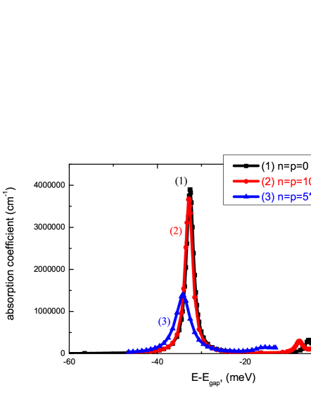
Fig. 1.: Calculated Hartree–Fock spectra for the quantum well with a width of 2.6 nm

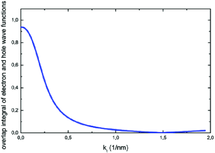
Fig. 2.: Overlap integral of the electron and hole wave functions

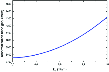
Fig. 3.: Dispersion of the renormalization band gap for the quantum well with a width of 2 nm at the concentration of carriers $5\times 10^{11}$ cm^-2

3 Results and Their Discussions

Numerically solving the microscopic polarization equations for the quantum well with a parabolic band, one can see that, with increasing the electron-hole gas density, the optical gain develops in the spectral region of the original exciton resonance. With increasing the free-carrier density, the ionization continuum shifts rapidly to longer wavelengths, while the 1$s$-exciton absorption line stays almost constant, due to the high degree of compensation between the weakening of the electron-hole binding energy and the band-gap reduction. Physically, this indicates the charge neutrality of an exciton [39]. The exciton absorption spectrum for the quantum well with a parabolic law of dispersion is presented in Fig. 1. All calculations are carried at a temperature of 300 K.

The overlap integral of the electron and hole wave functions is presented in Fig. 2.

Unlike will be develop the process of shifting of the absorption edge at a constant exciton energy with increasing the concentrations for the wurtzite quantum well. Solving the polarization equation in the Hartree–Fock approximation, one can find a red shift of the exciton resonance with increasing the concentration in the wurtzite quantum well. The calculated Hartree–Fock spectrum for the wurtzite quantum well with a width of 2 nm is presented in Fig. 4.

Such a shift can be explained by the difference between the overlap integrals of the electron and hole wave functions in the wurtzite quantum well and the quantum well with a parabolic band. The overlap integral of the electron and hole wave functions at nonzero wave vectors in the wurtzite quantum well has a smaller value than the overlap integral in the quantum well with a parabolic band. Due to this cause, the Coulomb renormalization of the electric dipole moment in (50) in the wurtzite quantum well is found to be smaller than that in the quantum well with a parabolic band and cannot compensate the Coulomb renormalization of the self-energy in (49), where it has the minus sign. This yields a shift of the exciton resonance to the side of less energies. Since the shift of the exciton resonance is a very rare effect, the examples of exceptions are always interesting.

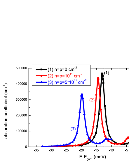
Fig. 4.: Calculated Hartree–Fock spectra for the quantum well with a width of 2 nm

Fig. 5.: Hartree gain spectrum (1) and Hartree–Fock gain spectrum (2) at the concentration of carriers $n=p=9\times 10^{12}$ cm^-2 for the quantum well with a width of 2 nm at the temperature 300 K

The dispersion of the renormalization band gap for the quantum well with a width of 2 nm at the concentration of carrier $5\times 10^{11}$ cm^-2 is presented in Fig. 3. The energy of the exciton resonance is calculated, and it is found that, for the concentration of carriers $5\times 10^{11}$ cm^-2, the exciton energy is equal to 3749.5 meV.

In general, the existence of the resonance and the Sommerfeld enhancement of a continuous optical spectrum is a reflection of the renormalization of the electric dipole interaction energy and is a cause of increasing the optical absorption in comparing with the optical spectrum of free carriers. This increase of the absorption is the example of a more general phenomenon of Coulomb enhancement and can be explained as follows. Due to the Coulomb attraction, an electron and a hole have a larger tendency to be located closer to each other, as compared with the case of noninteracting particles. This increase of the interaction duration leads to an increase of the optical transition probability and to the renormalization of the electric dipole interaction energy.

The Hartree and Hartree–Fock gain spectra are presented in Fig. 5.

Fig. 6.: Calculated energy spectra for heavy (hh1) and light (lh1) holes for the free valence band, Hartree energy spectra for heavy (hh2) and light (lh2) holes, and Hartree–Fock energy spectra for the heavy (hh3) and light (lh3) holes for the quantum well with a width of 2 nm at the concentration of carriers $n=p=9\times 10^{12}$ cm^-2 at the temperature 300 K

Fig. 7.: Calculated energy spectra for electrons (e1) for the free conduction band, Hartree energy spectra for electrons (e2), and Hartree–Fock energy spectra for electrons for the quantum well with a width of 2 nm at the concentration of carriers $n=p=$ $=9\times 10^{12}$ cm^-2 at the temperature 300 K

The energy spectra for heavy and light holes and for electrons in a quantum well, as well as the Hartree and Hartree–Fock renormalizations of the energy spectrum for heavy and light holes and electrons which reflect the many-body effect known as a renormalization of the band gap, are presented in Figs. 6 and 7.

4 Summary

The calculations of light gain spectra and exciton spectra were previously carried out only for the nitride quantum well with parabolic bands and not for quantum wells with compound bands. Here, we study the effect of nonparabolicity on exciton states in the wurtzite quantum well. We have calculated and explained that the exciton binding energy strongly depends on the mixing of valence bands, because it depends on the overlap integral of the electron and hole wave functions. We have calculated and explained a shift of the exciton resonance, which depends on the electron-hole gas concentration, and the gain spectrum shape in the wurtzite quantum well. We have found the exchange renormalization of the energy spectrum for holes and electrons. In the research of the influence of the overlap integral of wave functions on the Hartree–Fock renormalization of the electric dipole moment in the wurtzite quantum well, we conclude that a deviation from a parabolic band structure in the wurtzite quantum well leads to significant changes in the determination of the exciton binding energy. The calculations testify to a small change of the overlap integral of the electron and hole wave functions, which is caused by the intrinsic quantum confined Stark effect at the considered concentrations. The deviation from a parabolic band structure of the quantum well leads also to significant changes in the overlap integral of the electron and hole wave functions. This is the cause for a red shift of the exciton resonance with increasing the concentrations. The above-presented results can be explained by the influence of the valence band structure on quantum confined effects.

The author is grateful to Prof. V.A. Kochelap for numerous discussions.

Л.O. Локоть
ХАРТРI–ФОКIВСЬКА ЗАДАЧА
ЕЛЕКТРОННО-ДIРКОВОЇ ПАРИ
В КВАНТОВIЙ ЯМI GaN
Р е з ю м е
Розглянуто мiкроскопiчне обчислення спектра поглинання для системи $\textrm{GaN}/\textrm{Al}_{x}\textrm{Ga}_{1-x}\textrm{N}$ квантової ями. Тодi як структури квантової ями з параболiчним законом дисперсiї проявляють звичайне висвiтлювання екситону без змiни спектральної областi, то значне червоне змiщення екситонного резонансу знайдено для в’юрцитної квантовоямної структури. Обчислено енергiю екситонного резонансу для в’юрцитної квантової ями. Одержанi результати можуть пояснюватися впливом валентної зонної структури на ефекти квантового конфайнменту. Обчислено оптичний спектр пiдсилення в хартрi–фокiвськiй апроксимацiї. Обчислено зоммерфельдiвське пiдсилення. Обчислено червоне змiщення спектра пiдсилення в хартрi–фокiвськiй апроксимацiї вiдносно хартрiвського спектра пiдсилення.

References

[1]
N. Savage, Nature Photonics 1, 83 (2007).
[2]
A. Khan, K. Balakrishnan, and T. Katona, Nature Photonics 2,
77 (2008).
[3]
H. Kawanishi, M. Senuma, and T. Nukui, Appl. Phys. Lett. 89,
041126 (2006).
[4]
H. Kawanishi, M. Senuma, M. Yamamoto, E. Niikura, and T. Nukui,
Appl. Phys. Lett. 89, 081121 (2006).
[5]
J. Shakya, K. Knabe, K.H. Kim, J. Li, J. Y. Lin, and H. X. Jiang,
Appl. Phys. Lett. 86, 091107 (2005).
[6]
R.G. Banal, M. Funato, and Y. Kawakami, Phys. Rev. B. 79,
121308(R) (2009).
[7]
R.D. Meade, A.M. Rappe, K.D. Brommer, and J.D. Joannopoulos, J. Opt.
Soc. Am. B 10, 328 (1993).
[8]
S.H. Park, D. Ahn, and S.L. Chuang, IEEE J. Quantum Electron. 43, 1175 (2007).
[9]
M.F. Schubert, J. Xu, J.K. Kim, E.F. Schubert, M.H. Kim, S. Yoon,
S.M. Lee, C. Sone, T. Sakong, and Y. Park, Appl. Phys. Lett. 93, 041102 (2008).
[10]
M.H. Kim, W. Lee, D. Zhu, M.F. Schubert, J.K. Kim, E.F. Schubert,
and Y. Park, IEEE J. Sel. Top. Quantum Electron. 15, 1122
(2009).
[11]
S.H. Park, D. Ahn, and J.W. Kim, Appl. Phys. Lett. 92, 171115
(2008).
[12]
A.E. Romanov, T.J. Baker, S. Nakamura, J.S. Speck, and E.J.U. Group,
J. Appl. Phys. 100, 023522 (2006).
[13]
A.A. Yamaguchi, Appl. Phys. Lett. 94, 201104
(2009).
[14]
H.H. Huang and Y.R. Wu, J. Appl. Phys. 106, 023106
(2009).
[15]
M. Nido, Jpn. J. Appl. Phys., Part 2 34, L1513
(1995).
[16]
S. Chichibu, T. Azuhata, T. Sota, H. Amano, and I. Akasaki, Appl.
Phys. Lett. 70, 2085 (1997).
[17]
D. Fu, R. Zhang, B. Wang, Z. Zhang, B. Liu, Z. Xie, X. Xiu, H. Lu,
Y. Zheng, and G. Edwards, J. Appl. Phys. 106, 023714
(2009).
[18]
P.Y. Dang and Y.R. Wu, J. Appl. Phys. 108, 083108
(2010).
[19]
S. Fujita, T. Takagi, H. Tanaka, and S. Fujita, Phys. Status Solidi
B 241, 599 (2004).
[20]
W.J. Fan, J.B. Xia, P.A. Agus, S.T. Tan, S.F. Yu, and X.W. Sun, J.
Appl. Phys. 99, 013702 (2006).
[21]
S. Sasa, M. Ozaki, K. Koike, M. Yano, and M. Inoue, Appl. Phys. Lett
89, 053502 (2006).
[22]
K. Koike, I. Nakashima, K. Hashimoto, S. Sasa, M. Inoue, and M.
Yano, Appl. Phys. Lett 87, 112106 (2005).
[23]
S.-H. Park and S.-L. Chuang, J. Appl. Phys. 72, 3103
(1998).
[24]
M. Willatzen, IEEE Trans. Ultrason. Ferroelectr. Freq. Control 48, 100 (2001).
[25]
B.A. Auld, Acoustic Fields and Waves in Solids (Wiley, New
York, 1973).
[26]
L. Duggen and M. Willatzen, Phys. Rev. B 82, 205303
(2010).
[27]
M. Lindberg and S. W. Koch, Phys. Rev. B. 38, 3342
(1988).
[28]
W.W. Chow, S.W. Koch, and M. Sargent III, Semiconductor Laser
Physics (Springer, New York, 1994).
[29]
W.W. Chow, M. Kira, and S.W. Koch, Phys. Rev. B. 60, 1947
(1999).
[30]
W.W. Chow and M. Kneissl, J. Appl. Phys. 98, 114502
(2005).
[31]
G.L. Bir and G.E. Pikus, Symmetry and Strain-Induced Effects in
Semiconductors (Wiley, New York, 1974).
[32]
R.S. Knox, Theory of Excitons (New York, Academic Press,
1963).
[33]
L.O. Lokot, Ukr. J. Phys. 54, 963 (2009).
[34]
L.O. Lokot, Ukr. J. Phys. 57, 12 (2012).
[35]
M. Gell-Mann and K.A. Brueckner, Phys. Rev. 106, 364
(1956).
[36]
C. Kittel, Quantum Theory of Solids (Wiley, New York,
1963).
[37]
S. Raimes, Many-Electron Theory (North-Holland, Amsterdam,
1972).
[38]
R.D. Mattuck, A Guide to Feynman Diagrams in The Many-Body
Problem (McGraw-Hill, New York, 1967).
[39]
H. Haug and S. Schmitt-Rink, Prog. Quant. Electr. 9, 3
(1984).
Received 24.04.12