“Ping-pong” electron transfer.
II. Multiple reflections of the Loschmidt echo
and the wave function trapping by an acceptor.

Abstract

This paper continues the preceding paper on the problem of quantum dynamics on the lattice. Firstly we consider the multiple reflections of the wave function (Loschmidt echo). The phenomenon of wave function concentration on the impurity site after reflections is found. The solution representing the total amplitude $a(t)$ is obtained as the series in terms of partial amplitudes $a_{k}(t)$. The contribution of $k$th partial amplitude becomes dominant only after $k$th reflection from the lattice end. An excellent agreement between analytical and accurate numerical results is obtained. Next problem, – wave packet trapping by defects, is solved by numerical simulation. Analytical expressions are derived in few cases allowing to estimate the quantum efficiency of charge transfer. Obtained results can qualitatively explain recent experiments on the highly efficient charge transport in olygonucleotides and polypeptides.

PACS numbers: 87.15.-v; 42.15.Dp

Keywords: charge transport, Loschmidt echo, wave packet, DNA

^∗The corresponding author: gvin@deom.chph.ras.ru.

I Setting up a problem

For the completeness we repeat few details of the setting up the problem from the preceding paper, but in a somewhat different notations.

We consider quantum system consisting of $(N+1)$ sites. Most left site is an impurity site; other $N$ sites are reservoir. This system is defined by the $(N+1)\times(N+1)$ matrix hamiltonian

$$H=\begin{pmatrix}E&\overrightarrow{{\bf v}}\\ \overrightarrow{{\bf v}}&\widehat{\bf B}\\ \end{pmatrix},$$ (1)

where $E$ is the on-site energy of the impurity site; $\widehat{\bf B}$ is the $N\times N$ tridiagonal matrix of reservoir with matrix elements $B_{i,j}=\delta_{i,i+1}+\delta_{i,i-1}$; $\overrightarrow{{\bf v}}$ is the interaction of the impurity site with the reservoir and is chosen in the form $v_{i}=C\delta_{i,1}$. The wave function is $\overrightarrow{\Psi}(t)=\left\{a(t),\overrightarrow{\bf b}(t)\right\}=a(t),b_{1}(t),b_{2}(t),\ldots,b_{N}(t)$. Initial condition: $a(t=0)=1,\,\,\overrightarrow{{\bf b}}(t=0)=0$. The aim of this paper is to find the amplitude $a(t)$ on the impurity site as the result of multiple pave packet reflections (Loschmidt echo).

The dimensionless $(\hbar=1)$ Schrödinger equation is

$$\left\{\begin{split}i\dfrac{{\rm d}a(t)}{{\rm d}t}=&Ea(t)+(\overrightarrow{\bf v}\cdot\overrightarrow{\bf b});\qquad\qquad a(t=0)=1\\ i\dfrac{{\rm d}\overrightarrow{\bf b}(t)}{{\rm d}t}=&\left(\widehat{\bf B}\cdot\overrightarrow{\bf b}(t)\right)+\overrightarrow{\bf v}\,a(t);\qquad\overrightarrow{\bf b}(t=0)=0.\end{split}\right.$$ (2)

If vector $\overrightarrow{\bf b}$ is expanded in terms of the eigenfunctions $b_{k}(i)$ of matrix $\widehat{\bf B}$, then the following integro-differential equation can be obtained:

$$\dot{a}=-iEa-\int\limits_{0}^{t}B^{N}(t-\tau)\,a(\tau)\,{\rm d}\tau,\qquad a(t=0)=1,$$ (3)

with the kernel

$$B^{N}(t)=\sum\limits_{k=1}^{N}\exp(-i\varepsilon_{k}t)\left(\overrightarrow{\bf v}\cdot\overrightarrow{\bf b_{k}}\right)^{2}$$ (4)

and $\varepsilon_{k}$ is $k$th eigenvalue.

The Schrödinger equations (2) for this model are:

$$\left\{\begin{split}i\dot{a}=&\,Ea+Cb_{1}\\ i\dot{b}_{1}=&\,b_{2}+Ca\\ i\dot{b}_{2}=&\,b_{1}+b_{3}\\ \cdots\,\,\,\,&\,\,\,\,\cdots\cdots\cdots\\ i\dot{b}_{N}=&\,b_{N-1}\\ \end{split}\right.$$ (5)

with initial conditions $a(0)=1,\,\,b_{i=1,2,\ldots,N}(0)=0$. Eigenfunctions $\varepsilon(k)$ and eigenvalues $b_{i}(k)$ of the matrix $\widehat{\bf B}$ are well known:

$$\varepsilon(k)=2\,\cos\left(\dfrac{\pi k}{N+1}\right);\quad b_{k}(i)=\sqrt{\dfrac{2}{N+1}}\sin\left(\dfrac{\pi k}{N+1}i\right)\qquad k=1,2,\ldots,N.$$ (6)

The kernel $B^{N}(t)$ of Eq. (3), in accordance with (6), is defined by the following sum:

$$B^{N}(t)=\dfrac{2\,C^{2}}{N+1}\sum\limits_{k=1}^{N}\sin^{2}\left(\dfrac{\pi k}{N+1}\right)\,\exp\left[-2i\cos\left(\dfrac{\pi k}{N+1}\right)t\right].$$ (7)

II Expansion of $a(t)$ in terms of partial amplitudes

In the preceding paper we have shown that the well formed impulse with sharp forward front is generated at large times. The velocity of the impulse front $v=2$ is the maximal group velocity. If a lattice consists of $N$ sites, then the time of the first returning to the impurity site is $t\approx N$. And the cycle of $k$ returnings takes $t\approx kN$.

In this paper the detailed analysis of amplitude $a(t)$ in the time range $t\lesssim N$ was done. Now our goal is to find amplitude $a(t)$ on the impurity site at all times. We solve equation (3) with the kernel given by (7).

Bearing this in mind, the solution of (3) is searched as the expansion in terms of partial amplitudes $a_{k}(t)$. Each amplitude $a_{k}(t)$ is negligible in the time range $t\lesssim kN$ and its contribution to the total amplitude $a(t)$ becomes essential starting only from times $t\sim kN$.

In order to make sure in this possibility, the kernel $B^{N}(t)$ of Eq.  (7) should be transformed according to the Poisson formula:

$$\begin{split}B^{N}(t)=&\,C^{2}\sum\limits_{m=-\infty}^{m=+\infty}B_{m}(t),\quad{\rm where}\\ B_{m}(t)=&\,\dfrac{2}{\pi}\int\limits_{0}^{\pi}{\rm d}x\sin^{2}(x)\exp\left\{-2i[m(N+1)+t\cos(x)]\right\}.\end{split}$$ (8)

Note that $B_{m}(t)$ is the real function and there exists the explicit expression for $B_{0}(t)$ through the Bessel functions:

$$B_{0}(t)=J_{0}(2t)+J_{2}(2t).$$ (9)

The original equation (3) with regard to transformation (8) is rewritten in the form:

$$\dot{a}(t)=-iEa(t)-C^{2}\sum\limits_{m=-\infty}^{\infty}\int\limits_{0}^{t}B_{m}(t-t^{\prime})\,a(t^{\prime})\,{\rm d}t^{\prime}.$$ (10)

Note an important and useful property of functions $B_{m}$: every function $B_{m}(t)$ is small in the time range $0<t<mN$, such that

$$B_{m}(t)\approx\dfrac{\sin(2t)}{\pi[m(N+1)]^{3}},\quad m(N+1)-t\gg 1.$$ (11)

With a reasonable degree of accuracy one can say that the function $B_{m}(t)\approx 0$ when $t<mN$. Consequently, when $t<mN$, then only terms $B_{k}$ with indices $k<m$ are essential in the governing equation (10).

Now we represent amplitude $a(t)$ as the sum of partial amplitudes

$$a(t)=a_{0}(t)+a_{1}(t)+a_{2}(t)+\ldots\,.$$ (12)

Recall that our assumption concerning amplitudes $a_{k}(t)$ lies in the fact that amplitude $a_{k}(t)$ is small at $t<kN$. Their contribution to the total amplitude $a(t)$ becomes essential starting from time $t\sim kN$. To some extent $a_{k}(t)$ behaves like $B_{k}(t)$. Deriving an equation for $a_{k}(t)$, we assume that its right-hand side contains only terms $B_{m}(t)$ with $m\leq k$.

Prior to write down an equation for $a_{k}(t)$, we make one comment. Terms $B_{m}(t)$ are small (even for not too long lattices). This smallness is ensured by the fact that $B_{-m}(t)=B_{m}(-t)$. And $B_{m}(t)\sim(mN)^{-3}$ in the considered time range ($t>0$). Nevertheless these terms are taken into account as their accounting allows to derive explicit analytical formulaes.

Lets introduce following functions to account the contributions from $B_{m}(t)$ ($m<0$):

$$\widetilde{B}_{m}(t)=B_{m}(t)+B_{-m}(t),\quad m>0$$ (13)

and for uniformity of notations we set $\widetilde{B}_{0}(t)\equiv B_{0}(t)$.

Now in accordance with our assumptions, convert one equation (10) in a system of cycling equations for the partial amplitudes $a_{k}(t)$. Equation for $a_{0}(t)$ contains in the right-hand side only function $\widetilde{B}_{0}(t)$ (see (9)):

$$\dot{a}_{0}=-iEa_{0}-C^{2}\int\limits_{0}^{t}\widetilde{B}_{0}(t-t^{\prime})\,a_{0}(t^{\prime})\,{\rm d}t^{\prime},\quad a_{0}(0)=1.$$ (14)

and in accordance with the above-mentioned arguments, an equation for $a_{k}(t)$ ($k>0$) can be rewritten:

$$\dot{a}_{k}=-iEa_{k}-C^{2}\int\limits_{0}^{t}\sum\limits_{m=0}^{k}\widetilde{B}_{m}(t-t^{\prime})\,a_{k-m}(t^{\prime})\,{\rm d}t^{\prime},\quad a_{k}(0)=0\,\,(k>0).$$ (15)

It is notable that system (15) is accurate.

The Laplace transformation of (14) gives the following expression for $a_{0}(p)$:

$$a_{0}(p)=\dfrac{1}{p+iE+C^{2}\,\widetilde{B}_{0}(p)}.$$ (16)

Here $\widetilde{B}_{0}(p)$ is the Laplace transform of $B_{0}(t)$ (see (9)):

$$\widetilde{B}_{0}(p)=\dfrac{1}{2}\left(\sqrt{p^{2}+4}-p\right).$$ (17)

Recall that expression (16) is nothing else then amplitude $a(t)$ in the infinite lattice when there is no reflections.

The Laplace transformation of system (15) gives the algebraic system of recurrence relationships for $a_{k}(p)$ ($k>0$):

$$a_{k}(p)=-C^{2}\,a_{0}(p)\sum\limits_{m=0}^{k-1}\widetilde{B}_{k-m}(p)\,a_{m}(p).$$ (18)

The Laplace transform $\widetilde{B}_{m}(p)$ of the function $\widetilde{B}_{m}(t)$ (see (8)) is given by the integral:

$$\widetilde{B}_{m}(p)=\dfrac{2}{\pi}\int\limits_{0}^{t}\sin^{2}(y)\exp[-2im(N+1)y]\left[\dfrac{1}{p+2i\cos(y)}+\dfrac{1}{p-2i\cos(y)}\right]{\rm d}y.$$ (19)

An explicit form for the integral (19) can be obtained. With this aim in view, the integration contour should be deformed as shown in Fig. 1.

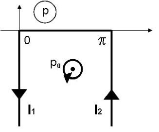
Figure 1: The integration along the path $[0,\,\pi]$ in expression (19) is changed to the residue in the pole $p_{0}$ and two integrals $I_{1}$ and $I_{2}$.

As the integrand in (19) has period $\pi$, integrals $I_{1}$ and $I_{2}$ are cancelled as they have opposite integration paths. Consequently $\widetilde{B}_{m}(p)$ is defined only by the pole contribution at the point $y_{0}$ ($\cos(y_{0})=ip/2$). Then we have:

$$\widetilde{B}_{m}(p)=\sqrt{4+p^{2}}\left[i\widetilde{B}_{0}(p)\right]^{2m(N+1)}.$$ (20)

Due to the fact that $\widetilde{B}_{m}(p)$ forms the geometrical progression by $m$, it is possibile to make an explicit summation in the recurrence formulaes (18). It is the reason why the total amplitude $a(t)$ can be represented in the form of the closed expression (this is done in Appendix).

The Laplace transforms of the partial amplitudes $a_{k}(p)$ ($k>0$) are expressed as

$$a_{k}(p)=-a_{0}(p)\,d\,(1-d)^{k-1}\left(i\widetilde{B}_{0}\right)^{2k(N+1)},\quad{\rm where}\quad d\equiv a_{0}\,C^{2}\sqrt{p^{2}+4}.$$ (21)

To get explicit expressions for the partial amplitudes, the inverse Laplace transform should be made. Transforming the Laplace integral to the integration path around the cut $[-2i,2i]$, one can get an expression for $a_{0}(t)$:

$$a_{0}(t)=\dfrac{1}{\pi}\int\limits_{-2}^{2}\exp(ixt)\,{\rm Im}\left\{\left[{x\left(1-\dfrac{C^{2}}{2}\right)+E-\dfrac{iC^{2}}{2}\sqrt{4-x^{2}}}\right]^{-1}\right\}{\rm d}x.$$ (22)

Further on we get the following expression for the partial amplitudes $a_{k}(t)$:

$$a_{k}(t)=-\dfrac{C^{2}}{\pi}\int\limits_{-2}^{2}\sqrt{4-x^{2}}\exp(ixt){\rm Re}\left[a_{0}^{2}\left(1-C^{2}a_{0}\sqrt{4-x^{2}}\right)^{k-1}\left(i\widetilde{B}_{0}\right)^{2k(N+1)}\right]{\rm d}x.$$ (23)

Here the Laplace transform for $a_{0}(p)$ (see (16) and (20)) are performed at $p=ix$. An analysis of expression for $a_{k}(t)$ shows that, as supposed, $a_{k}(t)\ll 1$ when $t<(k+1)N$.

Therefor, if the partial sum $a_{0}+a_{1}+\ldots a_{k}$ is taken for the representation of amplitude $a(t)$, then the error of such approximation is of the same order as the smallness of $\widetilde{B}_{k}(t)$ (see (11)), $\sim[k+1)(N+1)]^{-3}$.

Consider as an example very short lattice ($N=2$), and as an approximation – sum of only three partial amplitudes $a_{0}+a_{1}+a_{2}$. In Fig. 2 this partial sum is compared with the result of numerical integration of the Schrödinger equation (5). For $t<8$ the expected error is $\sim 5\cdot 10^{-5}$. Thus the representation of $a(t)$ by the sum of partial amplitudes is a very good approximation even for short lattices (an accuracy increases if lattice is longer).

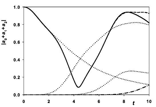
Figure 2: The comparison of the limited sum of partial amplitudes $a_{0}+a_{1}+a_{2}$ (solid line) with the numerical integration (dashed line). Dotted lines – partial amplitudes $a_{0}$, $a_{1}$, $a_{2}$ “starting” at times $t=0,\,2,\,4$, correspondingly. Small divergence is observe only at $t>8$ where the unaccounted partial amplitude $a_{4}$ (dash-dot line) starts to make the contribution. Parameters: $N=2,\,E=1,\,C=0.5$. Mean-square error (MSE) $\lesssim 10^{-3}$.

III Recursion. Multiple returning to the initial state.

If the lattice is long enough then partial amplitudes, following each other, have enough time to damp on the corresponding time range $[t\div t+N]$. In this case the partial amplitudes do not interfere and reproduce the total amplitude with very high accuracy (see Fig. 3). The maxima of returning amplitudes slowly decrease.

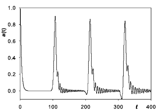
Figure 3: Sum of partial amplitudes $a_{0},\,a_{1},\,a_{2},\,a_{3}$ practically coincide with the total amplitude $a(t)$. Numerical results are not shown as they excellently coincide with analytical result (MSE $\lesssim 10^{-4}$). Parameters: $N=100,\,E=0,\,C^{2}=0.25$.

Partial amplitudes interfere in the short lattices and maxima of returning amplitudes are irregular. The dependence of the total amplitude $a(t)$ vs. time for the lattice with $N=10$ is shown in Fig. 4.

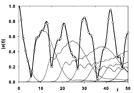
Figure 4: Solid line – sum of partial amplitudes $|a_{0}+a_{1}+\ldots,+a_{8}|$. It practically coincides with amplitude $a(t)$. Dots – partial amplitudes $a_{0},\,a_{1},\ldots,a_{8}$. Maximal value of returned amplitude is $\approx 0.95$ (at $t=42$). Main contributions to maximum give partial amplitudes $a_{2},\,a_{3},\,a_{4},\,a_{5},\,a_{6}$. Empty circles – numerical result. MSE $\lesssim 10^{-4}$. Parameters: $N=10,\,E=0,\,C^{2}=0.4$.

Numerical analysis performed at different values of parameters $C,\,E$ $N$ shows, that the maximal value of returned amplitude $a_{\rm ret}\approx\!0.972$ at $t=42$ for $N=10,\,E=0,\,C^{2}=0.4$,

Incident and reflected impulses interfere on short lattices and the degree of returning is difficult to analyze at arbitrary parameter values $C,\,E,\,N$. But the first returning (maximal value of the partial amplitude $a_{1}$) can be treated analytically if the lattice is long enough when amplitude $a_{0}$ becomes negligible.

The expression (23) for $a_{1}(t)$ using the trigonometric substitution of variables can be written:

$$a_{1}(t)=\dfrac{4C^{2}}{\pi}\int\limits_{0}^{\pi}\sin^{2}(x)\,\exp[2it\cos(x)]\,{\rm Re}\left\{\dfrac{\exp[2i(N+1)x]}{[2\cos(x)+E-C^{2}\exp(ix)]^{2}}\right\}{\rm d}x.$$ (24)

Fig. 5 shows the maximal values of amplitude calculated according to (24) at $E=0$ and different values of parameters $N$ and $C$. One can see that if $C^{2}\approx 0.2$ then the returned amplitude practically does not depend on the lattice length ($10<N<100$). The dissimilarity of the partial amplitude from the total amplitude is negligible on this time range ($N<t<2N$). Divergence becomes essential ($\sim$15%) for the shortest of considered lattices ($N=10$) and smallest value of parameter $C$ ($C^{2}=0.1$). Amplitude $a_{0}$ has no enough time to fully decay at these parameters values.

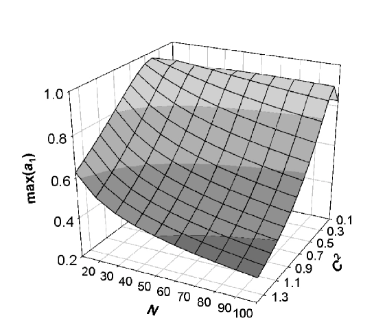
Figure 5: Maximal value of amplitude of the first returning at $E=0$ and different values of $C$ and $N$.

IV Wave packet trapping by an acceptor

The phenomenon of multiple reflections of the wave packet (Loschmidt echo) is unlikely to observe experimentally. The reason is that the wave function does not interact with environment. Below we consider the problem which mimics the experiments on the charge transfer (CN) in DNA where the wave function is irreversibly trapped by an acceptor. And the fraction of the wave function trapped by an acceptor is of primary interest of this section. This quantity can be compared with the quantum efficiency of CT.

Consider the lattice with the attached site (acceptor, see Fig. 6). The number of this site is $N_{\rm a}$. The acceptor has on-site energy $E_{\rm a}$ and the hopping integral $C_{\rm a}$. Amplitude of the wave function on the acceptor is labelled by $b_{\rm a}$. Initially we limit ourself by the weak bounding energy between the lattice and acceptor, i.e. $C_{\rm a}\ll 1$. This approximation allows to make necessary analytical estimations.

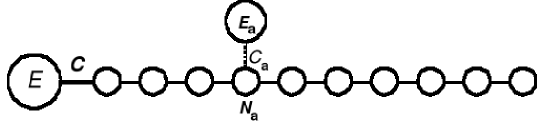
Figure 6: Schematic representation of the lattice with acceptor. Acceptor is attached to the lattice site with number $N_{\rm a}$ and has the on-site energy $E_{\rm a}$ and hopping integral (the interaction energy with the lattice) $C_{\rm a}$.

The system of equations (5) changes in an obvious way: an equation for the amplitude of the wave function on the acceptor is added:

$$i\dot{b}_{\rm a}(t)=E_{\rm a}b_{\rm a}(t)+C_{\rm a}b_{N_{\rm a}},\quad b_{\rm a}(t=0)=0.$$ (25)

The equation for the site $N_{\rm a}$ is also modified:

$$i\dot{b}_{N_{\rm a}}(t)=b_{N_{\rm a}-1}+b_{N_{\rm a}+1}+C_{\rm a}b_{\rm a}.$$ (26)

Other equations stay unchanged.

Staying in the frameworks of the initially formulated problem, consider now results obtained in numerical simulation in the case, when the acceptor is located close to the impurity site (donor). It turns our that the fraction of the wave function on the acceptor, being captured, stays on the acceptor for a long time. Fig. 7 shows this phenomenon for the lattice consisting of $N=100$ sites. (The time range is such, that the reflected impulse has no time to return back after reflection).

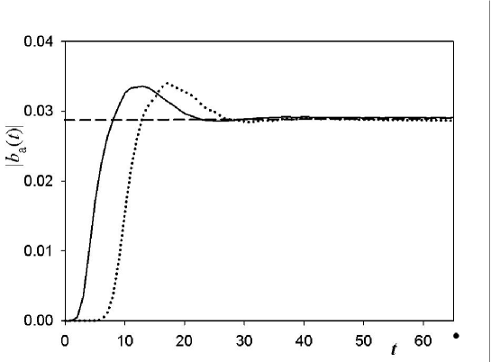
Figure 7: The dependence of the wave function amplitude on the acceptor $|b_{\rm a}(t)|$ for two positions of the acceptor on the lattice: $N_{\rm a}=5$ (solid line) and $N_{\rm a}=15$ (dots). Dashed line – expression (33). Parameters: $N=100,\,\,C=0.4,\,\,E=0.5,\,\,C_{\rm a}=0.02,\,\,E_{\rm a}=0.3$.

It is possible to estimate the dependence of the wave function amplitude on the acceptor vs. time in the approximation of the weak coupling ($C_{\rm a}\ll 1$). Note that in this approximation the acceptor affects the lattice very weakly. Therefor the lattice is not disturbed and it is described by Eq. (5). Amplitude of the wave function on the acceptor will be calculated according to the obvious expression resulting from (25):

$$b_{\rm a}(t)=-iC_{\rm a}\exp(-iE_{\rm a}t)\int\limits_{0}^{t}\exp(iE_{\rm a}\tau)b_{N_{\rm a}}\,{\rm d}\tau.$$ (27)

Fig.  8 shows the comparison of two solutions of the Schrödinger equation: accurate (expression (5) ) and approximate (equation (25)). One can see that these solutions differ very little and an approximation by the unperturbed lattice is very good.

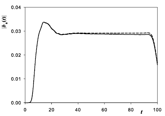
Figure 8: A comparison of the accurate and approximate solutions for the acceptor attached to the tenth lattice site ($N_{\rm a}=10$). Solid line – accurate solution (an influence of the acceptor on the lattice is accounted). Dashed line – unperturbed lattice. Parameters: $N=100,\,\,N_{\rm a}=10,\,\,C=0.4,\,\,E=0.5,\,\,C_{\rm a}=0.02,\,\,E_{\rm a}=0.3$.

Analytically will be considered the case when time is large enough such that amplitude $a(t)$ on the impurity site decreased practically to zero. It means that the lattice is long and time is large, and the impulse and its tail went away from the acceptor. Then the lattice can be considered as having infinite length.

As is seen from (27), it is necessary to evaluate integral $\int_{0}^{t}\exp(iE_{\rm a}\tau)b_{N_{\rm a}}\,{\rm d}\tau$ (the phase multiplier $\exp(-iE_{\rm a}t)$ is unessential for the modulus of the wave function). We consider the amplitude on acceptor in the limit $t\to\infty$.

To evaluate the integrals, system (5) should be multiplied by $\exp(iEt)$ and integrated in the limits from 0 to $\infty$. Lets introduce the notations:

$$I_{0}\equiv\int\limits_{0}^{\infty}\exp(iE_{\rm a}\tau)a(\tau){\rm d}\tau,\qquad I_{k}\equiv\int\limits_{0}^{\infty}\exp(iE_{\rm a}\tau)b_{k}(\tau){\rm d}\tau.$$ (28)

Then for $I_{k}$ we get the recurrence relations:

$$\begin{split}CI_{1}=&\,-i+(E-E_{\rm a})I_{0}\\ I_{2}=&\,\,E_{\rm a}I_{1}-CI_{0}\\ I_{3}=&\,\,E_{\rm a}I_{2}-I_{1}\\ I_{4}=&\,\,E_{\rm a}I_{3}-I_{2}\\ \ldots&\,\,\ldots\,\ldots\end{split}$$ (29)

Amplitude $a(t)$ on the impurity site in the considered approximation is $a_{0}(t)$ and integral $I_{0}$ is the Laplace transform $a_{0}(p)\,\,(p=iE_{\rm a})$. As the result we get:

$$I_{0}=\left[i(E-E_{\rm a})+C^{2}\exp(i\phi)\right]^{-1},\qquad\phi=\arcsin(E_{\rm a}/2).$$ (30)

System of equations (29) has the following solution:

$$I_{k}=CI_{0}\left[-i\exp(i\phi)\right]^{k}.$$ (31)

Thus the limiting values of the acceptor amplitudes (with the accuracy of oscillating multiplier $\exp(-iEt)$) on different sites are$-iC_{\rm a}I_{k}$ (see (26)) and differ only by phase multiplier. In this case the amplitude on acceptor is

$$b_{\rm a}(t)\approx-iC_{\rm a}C\exp(-iE_{\rm a}t)I_{0}\,\exp[-i\exp(i\phi)]^{k}.$$ (32)

If the phase multipliers, unessential for the amplitude of the wave function, are eliminated, then the amplitude is

$$b_{\rm a}(t)\approx\dfrac{C_{\rm a}C}{i(E-E_{\rm a})+C^{2}\exp(i\phi)},\qquad\phi=\arcsin(E_{\rm a}/2).$$ (33)

Fig. 7 demonstrates that the limiting value of amplitude coincides with the numerical calculation.

It follows from (33) that at fixed values of the hopping integrals $C$ and $C_{\rm a}$, maximal value of $b_{\rm a}$ is achieved in “resonance” values of $E$ and $E_{\rm a}$, when $E=E_{\rm a}$. In this resonance case $b_{\rm a}(t)\approx C_{\rm a}/C$.

If times are such that the impulse reflects, returns and passes by the acceptor, then the amplitude variations are irregular and depend on the acceptor location on the chain (see Fig.9).

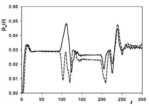
Figure 9: Amplitude of the wave function on acceptor when $N_{\rm a}=5$ (solid line) and $N_{\rm a}=10$ (dashed line). Time is such that the double reflection occurs. Parameters: $N=100,\,\,C=0.4,\,\,E=0.5,\,\,C_{\rm a}=0.02,\,\,E_{\rm a}=0.3$.

There was considered above the cases, when the bounding of the acceptor with the lattice is weak. But practically, for the efficient charge transfer, it is necessary to obtain the conditions when the degree of the CT is higher, i.e. parameter $C_{\rm a}$ should be larger. The value $E_{\rm a}$ also plays some role.

Below we consider few examples when parameter $C_{\rm a}$ has comparatively large value. Fig. 10 shows the dependence of the wave function amplitude on the acceptor, when the hopping integral $C_{\rm a}=0.1$. The amplitude becomes well larger and reaches value $|b_{\rm a}|\lesssim 0.2$.

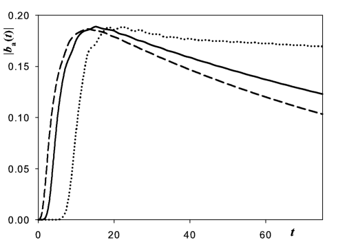
Figure 10: Dependence of the wave function amplitude on the acceptor vs. time for few locations of the acceptor on the lattice. $N_{\rm a}=2$ (dashed line), $N_{\rm a}=5$ (solid line) $N_{\rm a}=15$ (dots). Parameters: $N=100,\,\,C=0.5,\,\,E=0.5,\,\,C_{\rm a}=0.1,\,\,E_{\rm a}=0.5$. (According to (33) the value $b_{\rm a}=0.2$).

In the case of the total resonance (when $E=E_{\rm a}$ and $C=C_{\rm a}$), amplitude $|b_{\rm a}|$ becomes even more and this case is shown in Fig. 11.

From two latter figures it follows that the acceptor population can change significantly depending on the parameters. When the population is small (Fig. 10) then time of life is comparatively large. And on contrary, time of life is small when population is large (Fig. 11). This peculiarity has natural explanation: the larger is the acceptor bounding with the lattice the shorter is time of life.

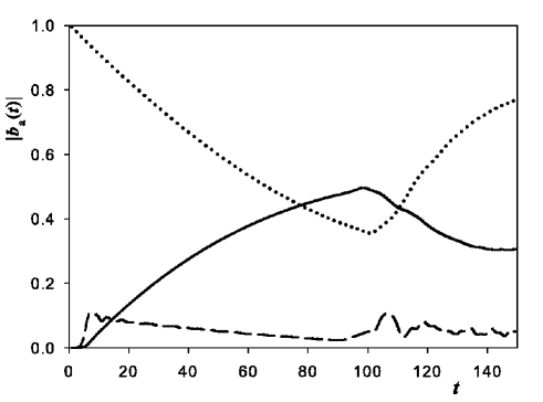
Figure 11: Dependence of the wave function amplitudes vs. time on the acceptor $|b_{\rm a}(t)|$ (solid line), on the impurity site $|a(t)|$ on the left lattice end (dots) and on the acceptor site $|b_{10}(t)|$ (dashed line). Parameters: $N=100,\,\,C=0.1,\,\,E=0.5,\,\,C_{\rm a}=0.1,\,\,E_{\rm a}=0.5$.

And finally we consider the case when an acceptor is located on the right lattice end ($N$th site is an acceptor) (see Fig. 12). It is seen that the amplitude on acceptor is rather large ($|b_{\rm a}|\approx 0.35$), and, what is very important, does not depend on the lattice length. Moreover, time dependencies for the amplitude decay are practically identical. This result is in good agreement with experiments on the charge transfer in synthetic DNA and polypeptides where the CT probability does not depend on the distance.

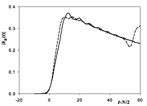
Figure 12: Dependence of the wave function amplitude on the acceptor (located on the right lattice end) vs. time for two lattice lengths: $N=100$ (solid line) and $N=50$ (dashed line). The time point of reference is shifted back by the value $N/2$ for the data comparison. Parameters: $C=0.5,\,\,E=0.5,\,\,C_{\rm a}=0.1,\,\,E_{\rm a}=0.5$.

An estimation of typical time scale is necessary. It has to be done to understand how long the wave function stays in the bounded state, and is this time enough for photophysical or electrochemical response for the charge registration. The typical dynamical time (period of one vibration) is $[t]_{\rm d}\approx 1.7\cdot 10^{-13}$ s Con00 ; Con03 . The typical electronic time (time unit in this work) is approximately two orders of magnitude shorter $[t]_{\rm e}\approx 2.2\cdot 10^{-15}$ s Ast12a . As is shown above, the wave function can stay on the acceptor during dozens time units, what is $\sim$ps. In many cases this time is enough for effective charge trapping by an acceptor with following registration.

V Conclusions

In two papers we thoroughly analyzed the quantum dynamics of the excitation (electronic wave function) propagation (first part), reflection and trapping (second part). The system consists of the homogeneous one-dimensional lattice with the impurity site, and an excitation initially is totally localized on the impurity site.

A rather unexpected results consists in the fact that initially localized wave function starts to move spontaneously forming well defined wave packet. After first reflection wave packet is again concentrated on the impurity site with the amplitude $\gtrsim 90$% of initial amplitude. This process repeats many times.

To describe multiple reflections of the wave packet an useful approach consisting in the representation of the full wave function on the impurity site $a(t)$ through the partial amplitudes $a_{k}(t)$.

The temporal evolution of the wave function is described with very high accuracy up to dozens reflection. The interference of falling and reflected impulses occurs after these large times, which is difficult to take into account analytically. The behavior of the quantum dynamical system is regular in this time range. The behavior on large times needs further detailed consideration.

Results on the wave function trapping by an acceptor can explain recent results on the efficient ballistic charge transport in synthetic DNA and polypeptides.

Appendix A

Original equation for the amplitude $a(t)$ has the form (see (3)):

$$\dot{a}=-iEa-\int\limits_{0}^{t}B^{N}(t-\tau)\,a(\tau){\rm d}\tau,\quad a(t=0)=1.$$ (34)

The solution of this equation for the Laplace transform $a(p)$ is:

$$a(p)=\dfrac{1}{p+iE+B^{N}(p)}.$$ (35)

The Poisson representation for the kernel $B^{N}(p)$ has form (see (8), (17), (20)):

$$\begin{split}B^{N}(p)=&\,C^{2}\sum\limits_{m=0}^{\infty}\widetilde{B}_{m}(p)\\ \widetilde{B}_{0}(p)=&\,\dfrac{1}{2}\left(\sqrt{p^{2}+4}-p\right)\\ \widetilde{B}_{m}(p)=&\,\sqrt{p^{2}+4}\,[b(p)]^{2m(N+1)},\quad m>0\\ \end{split}$$ (36)

where the notation

$$b(p)\equiv\left(i\widetilde{B}_{0}(p)\right)^{2k(N+1)}$$ (37)

is introduced. As values $\widetilde{B}_{m}$ form the geometrical progression, we get:

$$B^{N}(p)=C^{2}B_{0}(p)+C^{2}\sqrt{p^{2}+4}\dfrac{b(p)}{1-b(p)}.$$ (38)

And the final expression for the total amplitude is:

$$a(p)=a_{0}\dfrac{1-b(p)}{1+b(p)\left(C^{2}a_{0}(p)\sqrt{p^{2}+4}-1\right)}.$$ (39)

An expansion into series in terms by $b(p)$ gives Laplace transforms of partial amplitudes. By this means it was not necessary to construct the system of the recurrence relations for the partial amplitudes, but simply use the expansion $a(p)$ (see (39)) into series in terms by $b(p)$. But this approach is valid only for the considered model where the necessary summation is possible and the compact expression for the kernel $B^{N}$ can be written. The method suggested in the paper of the expansion into series by partial amplitudes can be applied in other problems.

The back Laplace transformation gives the desired expression for $a(t)$:

$$a(t)=\dfrac{1}{2\pi}\int\limits_{-\infty}^{\infty}a(p){\rm d}p,\quad p=\Delta+i\omega,\quad\Delta>0.$$ (40)

Numerically it was verified that expression (39) gives accurate results.

It worth noting one intriguing property. If the integral (40) is closed around the cut $[-2i,\,2i]$, then the result (difference of integrals taken along banks of the cut) is zero. It was found numerically. And it follows that the function $a(p)$ has poles in the complex plane. And amplitude $a(t)$ can be obtained as the sum of residues in these poles. Additional analysis is necessary to throw light on this fact.

References

(1) E.M. Conwell, S.V. Rakhmanova. Proc. Natl.
Acad. Sci. USA 2000. 97, 4556.