Synchronization theory of microwave induced zero-resistance states

Abstract

We develop the synchronization theory of microwave induced zero-resistance states (ZRS) for two-dimensional electron gas in a magnetic field. In this theory the dissipative effects lead to synchronization of cyclotron phase with driving microwave phase at certain resonant ratios between microwave and cyclotron frequencies. This synchronization produces stabilization of electron transport along edge channels and at the same time it gives suppression of dissipative scattering on local impurities and dissipative conductivity in the bulk, thus creating the ZRS phases at that frequency ratios. The electron dynamics along edge and around circular disk impurity is well described by the Chirikov standard map. The theoretical analysis is based on extensive numerical simulations of classical electron transport in a strongly nonlinear regime. We also discuss the value of activation energy obtained in our model and the experimental signatures that could establish the synchronization origin of ZRS.

I Introduction

The experiments on resistivity of high mobility two-dimensional electron gas (2DEG) in presence of a relatively weak magnetic field and microwave radiation led to a discovery of striking Zero-Resistance States (ZRS) induced by a microwave field by Mani et al. mani2002 and Zudov et al. zudov2003 . Other experimental groups also found the microwave induced ZRS in various 2DEG samples (see e.g. dorozhkin ; smet ; bykov ). A similar behavior of resistivity is also observed for electrons on a surface of liquid helium in presence of magnetic and microwave fields konstantinov ; adc . These experimental results obtained with different systems stress the generic nature of ZRS. Various theoretical explications for this striking phenomenon have been proposed during the decade after the first experiments mani2002 ; zudov2003 . An overview of experimental and theoretical results is give in the recent review dmitrievrmp .

In our opinion the most intriguing feature of ZRS is their almost periodic structure as a function of the ratio $j=\omega/\omega_{c}$ between the microwave frequency $\omega$ and cyclotron frequency $\omega_{c}=eB/mc$. (in the following we are using units with electron charge $e$ and mass $m$ equal to unity). Indeed, a Hamiltonian of electron in a magnetic field is equivalent to an oscillator, it has a magneto-plasmon resonance at $j=1$ but in a linear oscillator there are no matrix elements at $j=2,3,...$ and hence a relatively weak microwave field is not expected to affect electron dynamics and resistivity properties of transport. Of course, one can argue that impurities can generate harmonics being resonant at high $j>1$ but ZRS is observed only in high mobility samples and thus the density of impurities is expected to be rather low. It is also important to note that ZRS appears at high Landau levels $\nu\sim 50$ so that a semiclassical analysis of the phenomenon seems to be rather relevant.

In this work we develop the theoretical approach proposed in adcdls . This approach argues that impurities produce only smooth potential variations inside a bulk of a sample so that ZRS at high $j$ appear from the orbits moving along sharp sample boundaries. It is shown adcdls that collisions with boundaries naturally generate high harmonics and that a moderate microwave field gives stabilization of edge channel transport of electrons in a vicinity of $j\approx j_{r}=1+1/4,\;2+1/4,\;3+1/4...$ producing at these $j$ a resistance going to zero with increasing microwave power. This theory is based on classical dynamics of electrons along a sharp edge. The treatment of relaxation processes is modeled in a phenomenological way by a dissipative term in the Newton equations. Additional noise term in the dynamical equations takes into account thermal fluctuations. The dissipation leads to synchronization of cyclotron phase with a phase of microwave field producing stabilization of edge transport along the edges in a vicinity of resonant $j_{r}$ values. Thus, according to the edge stabilization theory adcdls the ZRS phase is related to a universal synchronization phenomenon which is a well established concept in nonlinear sciences pikovsky .

While the description of edge transport stabilization adcdls captures a number of important features observed in ZRS experiments it assumes that the contribution of bulk orbits in transport is negligibly small. This assumption is justified for smooth potential variations inside the bulk of a sample. However, a presence of isolated small scale scatterers inside the bulk combined with a smooth potential component can significantly affect the transport properties of electrons (see e.g. alikbyk ). Also the majority of theoretical explanations of ZRS phenomenon considers only a contribution of scattering in a bulk dmitrievrmp . Thus it is necessary to analyze how a scattering on a single impurity is affected by a combined action of magnetic and microwave fields. In this work we perform such an analysis modeling impurity by a rigid circular disk of finite radius. We show that the dynamics in a vicinity of disk has significant similarities with dynamics of orbits along a sharp edge leading to appearance of ZRS type features in a resistivity dependence on $j$.

The paper is composed as follows: in Section II we discuss the dynamics in edge vicinity, in Section III we analyze scattering on a single disk, in Section IV we study scattering on many disks when their density is low, here we determine the resistivity dependence on $j$ and other system parameters, physical scales of ZRS effects are analyzed in Section V, effects of two microwave driving fields and other theory predictions are considered in Section VI, discussion of the results is given in Section VII.

We study various models which we list here for a reader convenience: wall model described by the Newton equations (1), (2) with microwave field polarization perpendicular to the wall (model (W1) equivalent to model (1) in adcdls ); the Chirikov standard map description (3) of the wall model dynamics called model (W2) (equivalent to model (2) in adcdls at parameter $\rho=1$); the single disk model with radial microwave field called model (DR1); the Chirikov standard map description (3) of model (DR1) called model (DR2) (here $v_{y}\rightarrow v_{r}$ in (3), $\rho>1$); the model of a single disk in a linearly polarized microwave field and static electric field called model (D1); the model of transport in a system with many disks called model (D2) which extends the model (D1); extension of model (D2) with disk roughness and dissipation in space called model (D3); the wall model (W2) extended to two microwave fields is called model (W3).

II Dynamics in edge vicinity

We remind first the approach developed in adcdls . Here, the classical electron dynamics is considered in a proximity of the Fermi surface and in a vicinity of sample edge modeled as a specular wall. The motion is described by Newton equations

$$d\mathbf{v}/dt=\mathbf{\omega_{c}}\times\mathbf{v}+\omega\vec{\epsilon}\cos\omega t-\gamma(v)\mathbf{v}+I_{ec}+I_{s}$$ (1)

where a dimensionless vector $\vec{\epsilon}=e\mathbf{E}/(m\omega v_{F})$ describes microwave driving field $\mathbf{E}$. Here an electron velocity $v$ is measured in units of Fermi velocity $v_{F}$ and $\gamma(v)=\gamma_{0}(|\mathbf{v}|^{2}-1)$ describes a relaxation processes to the Fermi surface. We also use the dimensionless amplitude of velocity oscillations induced by a microwave field $\epsilon=e|\mathbf{E}|/(m\omega v_{F})$. As in adcdls , in the following we use units with $v_{F}=1$. The last two terms $I_{ec}$ and $I_{s}$ in (1) account for elastic collisions with the wall and small angle scattering. Disorder scattering is modeled as random rotations of $\mathbf{v}$ by small angles in the interval $\pm\alpha_{i}$ with Poissonian distribution over time interval $\tau_{i}=1/\omega$. The amplitude of noise is assumed to be relatively small so that the mean free path $\ell_{e}$ is much larger than the cyclotron radius $r_{c}=v_{F}/\omega_{c}$. We note that the dissipative term is also known as a Gaussian thermostat hoover or as a Landau-Stuart dissipation pikovsky . The dynamical evolution described by Eq. (1) is simulated numerically using the Runge-Kutta method. Following adcdls we call this system model (W1) (equivalent to model (1) in adcdls ).

We note that for typical experimental ZRS parameters we have: electron density $n_{e}=3.5\cdot 10^{11}cm^{-2}$, effective electron mass $m=0.065m_{e}$, microwave frequency $f=\omega/2\pi=50GHz$, Fermi energy $E_{F}=mv_{F}^{2}/2=\pi n_{e}\hbar^{2}/m=0.01289V$, corresponding to $E_{F}/k_{B}=149.5Kelvin$, with Fermi velocity $v_{F}=2.641\cdot 10^{7}cm/s$. At such a frequency the cyclotron resonance $\omega=\omega_{c}=eB/mc$ takes place at $B=0.1161Tesla$ with the cyclotron radius $r_{c}=v_{F}/\omega_{c}=0.8873\mu m$. At such a magnetic field we have the energy spacing between Landau levels $\hbar\omega=\hbar\omega_{c}=0.2067mV=2.40K\cdot k_{B}$ corresponding to a Landau level $\nu=E_{F}/\hbar\omega_{c}\approx 62$. For a microwave field strength $E=1V/cm$ we have the parameter $\epsilon=eE/(m\omega v_{F})=0.003261$. With these physical values of system parameters we can always recover the physical quantities from our dimensionless units with $m=e=v_{F}=1$.

Examples of orbits running along the edge of specular wall are given in adcdls (see Fig.1 there). A microwave field creates resonances between the microwave frequency $\omega$ and a frequency of nonlinear oscillations of orbits colliding with the wall. Due to a specular nature of this collisions the electron motion has high harmonics of cyclotron frequency that leads to appearance of resonances around $j=1,2,3,4...$ (there is an additional shift of approximate value $1/4$ to $j_{r}$ values due to a finite width of nonlinear resonance).

To characterize the dynamical motion it is useful to construct the Poincaré section following the standard methods of nonlinear systems chirikov ; lichtenberg . We consider the Hamiltonian case at $\gamma_{0}=0$ in absence of noise. Also we choose a linear polarized microwave field being perpendicular to the wall which is going along $x$-axis (same geometry as in adcdls ). In this case the generalized momentum $p_{x}=v_{x}+By=y_{c}$ is an integral of motion since there are no potential forces acting on electron along the wall (here we use the Landau gauge with a vector potential $A_{x}=By$). The momentum $p_{x}$ determines a distance $y_{c}$ between a cyclotron center and the wall, which also remains constant in time. The Hamiltonian of the system has the form:

$$H=p_{y}^{2}/2+(p_{x}-By)^{2}/2+\epsilon\omega y\cos\omega t+V_{w}(y)\;,$$ (2)

where $V_{w}(y)$ is the wall potential being zero or infinity for $y<0$ or $y\geq 0$. Thus, we have here a so called case of one and half degrees of freedom (due to periodic time dependence of Hamiltonian on time) and the Poincaré section has continuous invariant curves in the integrable regions of phase space chirikov ; lichtenberg .

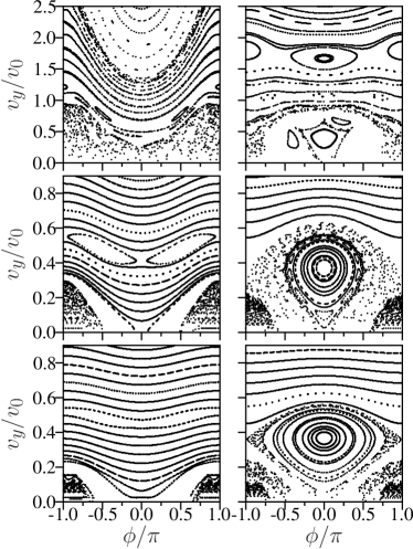
Figure 1: Poincaré sections of Hamiltonian (2) for $j=7/4$ (left column) and $j=9/4$ (right column) and different amplitudes of microwave field $\epsilon=0.02,0.04,0.2$ (from bottom to top). Here, the integral $p_{x}/mv_{F}=1$, trajectories start from wall with fixed $v_{x}=p_{x}=v_{0}=1$. Data for model (W1) at $\gamma_{0}=0$, $\alpha_{i}=0$.

The Poincaré sections for (1), (2) at $j=7/4,9/4$ and various amplitudes of microwave field $\epsilon$ are shown in Fig. 1. It shows a velocity $v_{y}$ at moments of collision with the wall at $y=0$ as a function of microwave phase $\phi=\omega t$ at these moments of time. All orbits initially start at the wall edge $y=0$ with the initial velocity $v_{x}=v_{0}=p_{x}=y_{c}$. The value of $p_{x}=y_{c}$ is the integral of motion. However, the kinetic energy of electron $E_{k}=(v_{x}^{2}+v_{y}^{2})/2$ varies with time. We see that at a small $\epsilon=0.02$ the main part of the phase space is covered by invariant curves corresponding to integrable dynamics. However, a presence of chaotic component with scattered points is also visible in a vicinity of separatrix of resonances, especially at large $\epsilon=0.2$. The points at $v_{y}$ close to zero correspond to orbits only slightly touching the wall, while the orbits at $v_{y}/v_{0}\gg 1$ have a large cyclotron radius and collide with the wall almost perpendicularly. There are also sliding orbits which have the center of cyclotron orbit inside the wall $(y_{c}>0)$ but we do not discuss they here. Indeed, the orbits, which only slightly touch the wall ($y_{c}\approx-v_{F}/\omega_{c}$), play the most important role for transport since the scattering angles in the bulk are small for high mobility samples and an exchange between bulk and edge goes via such type of dominant orbits adcdls .

We note that the section of Fig. 1 at $j=9/4$, $\epsilon=0.02$ is in a good agreement with those shown in Fig.1b of adcdls . However, here we have single invariant curves while in adcdls the curves have a certain finite width. This happens due to the fact that in adcdls the Poincaré section was done with trajectories having different values of the integral $p_{x}=y_{c}$ that gave some broadening of invariant curves. For a fixed integral value we have no overlap between invariant curves as it is well seen in Fig. 1 here.

The phase space in Fig. 1 has a characteristic resonance at a certain $v_{y}/v_{0}$ value which position depends on $j$ adcdls . An approximate description of the electron dynamics and phase space structure can be obtained on a basis of the Chirikov standard map chirikov ; lichtenberg ,scholar . In this description developed in adcdls an electron velocity has an oscillating component $\delta v_{y}=\epsilon\sin\omega t$ (assuming that $\omega>\omega_{c}$) and a collision with the wall gives a change of modulus of $v_{y}$ by $2\delta v_{y}$ (like a collision with a moving wall). For small collision angles the time between collisions is $\Delta t=2(\pi-v_{y})/\omega_{c}$. Indeed, $2\pi/\omega_{c}$ is the cyclotron period. However, the time between collisions is slightly smaller by an amount $2v_{y}/\omega_{c}$: at $v_{y}\ll v_{x}\approx v_{F}$ an electron moves in an effective triangular well created by the Lorentz force and like for a stone thrown against a gravitational field this gives the above reduction of $\Delta t$ (formally this expression for $\Delta t$ is valid for sliding orbits but for orbits slightly touching the wall we have the same $\Delta t$ but with minus that gives the correction $-2v_{y}/\omega_{c}$). The same result can be obtained via semiclassical quantization of edge states developed in avishai . It also can be found from a geometric overlap between the wall and cyclotron circle. This yields an approximate dynamics description in terms of the Chirikov standard map chirikov :

$${\bar{v}_{y}}=v_{y}+2\epsilon\sin\phi+I_{cc},\;{\bar{\phi}}=\phi+2(\pi-{\bar{v}_{y}/\rho})\omega_{/}\omega_{c}\;,$$ (3)

with the chaos parameter $K=4\epsilon\omega/(\rho\omega_{c})$. Usually we are in the integrable regime with $K<1$ due to small values of $\epsilon$ used in experiments. A developed chaos appears at $K>1$ chirikov ; lichtenberg . Here bars mark the new values of variables going from one collision to a next one, $v_{y}$ is the velocity component perpendicular to the wall, $\phi=\omega t$ is the microwave phase at the moment of collision. Here we introduced a dimensionless parameter $\rho$ which is equal to $\rho=1$ for the case of the wall model $W2$ considered here. However, we will show that for the dynamics around disk with a radial field in model (DR1) we have the same map (3) with $\rho=1+r_{c}/r_{d}$. Due to that it is convenient to write all formula with $\rho$. We note that a similar map (3) describes also a particle dynamics in a one-dimensional triangular well and a monochromatic field bubblon .

The term $I_{cc}=-\gamma_{c}v_{y}+\alpha_{n}$ in (3) describes dissipation and noise. The later gives fluctuations of velocity $v_{y}$ at each iteration ($-\alpha<\alpha_{n}<\alpha$; corresponding to random rotation of velocity vector in (1)). Damping from electron-phonon and electron-electron collisions contribute to $\gamma_{c}$. The Poincaré sections of this map are in a good agreement with those obtained from the Hamiltonian dynamics as it is seen in Fig. 1 here and Fig.1 in adcdls . Following adcdls we call this system model (W2) (equivalent to model (2) in adcdls ).

A phase shift of $\phi$ by $2\pi$ does not affect the dynamics and due to that the phase space structure changes periodically with integer values of $j$. Indeed, the position of the main resonance corresponds to a change of phase by an integer number of $2\pi$ values ${\bar{\phi}}-\phi=2\pi m=2(\pi-v_{y}/\rho)\omega/\omega_{c}$ that gives the position of resonance at $v_{res}=v_{y}=\pi\rho(1-m\omega_{c}/\omega)=\pi\rho\delta j/j$ where $m$ is the nearest integer of $\omega/\omega_{c}$ and $\delta j$ is the fractional part of $j$. Due to this relation we have the different resonance position for $j=7/4$ and $9/4$ being in agreement with the data of Fig. 1 at small values of $\epsilon$ when nonlinear corrections are small (we have here $\rho=1$). Thus at $j=9/4$ we have the resonance position at $v_{y}=0.1111\pi\approx 0.35$ in agreement with Fig. 1 (right bottom panel). For $j=2$ we have $v_{y}=0$ and at $j=7/4$ the resonance position moves to negative value $v_{y}=-0.45$. Thus, at $j=2;7/4$ the resonance separatrix easily moves particles out from the edge at $v_{y}<0$ where they escape to the bulk due to noise. In contrast at $j=9/4$ particles move along separatrix closer to the edge being then captured inside the resonance which gives synchronization of cyclotron phase with the microwave phase. This mechanism stabilizes the transmission along the edge.

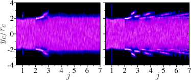
Figure 2: (Color online) Density distribution $w$ of electrons as a function of their dimensionless cyclotron center position $y_{c}/r_{c}$ between two walls and the frequency ratio $j=\omega/\omega_{c}$. The distance between specular walls is $6r_{c}$. The amplitude of microwave field is $\epsilon=0.1$ with polarization parallel (left panel) and perpendicular (right panel) to the walls (see text for more details). Here $\gamma_{0}/\omega=0.05$, $\alpha_{i}=0.01$, $\tau_{i}=1/\omega$, The variation of $j=\omega/\omega_{c}$ is obtained by changing magnetic field ($\omega_{c}=B$) keeping $\omega=const$; 100 electrons are simulated at each $j$ up to time $t_{r}=10^{5}/\omega$. Density is proportional to color changing from zero (black) to maximal density (white). Data for model (W1).

In adcdls it is shown that the orbits started in edge vicinity are strongly affected by a microwave field that leads to ZRS type oscillations of transmission along the edge and longitudinal resistivity $R_{xx}$. The ZRS structure appears both in the frame of dynamics described by (1) (model (W1)) and map description (3) (model (W2)). The physical mechanism is based on synchronization of a cyclotron phase with a phase of microwave driving that leads to stabilization of electron transport along the edge. An extensive amount of numerical data has been presented in adcdls and we think there is no need to add more. Here, we simply want to illustrate that even those orbits which start in the bulk are affected by this synchronization effect. For that we take a band of two walls with a band width between them being $\Delta y=L=6r_{c}$. Initially 100 trajectories are distributed randomly in a bulk part between walls when a cyclotron radius is not touching the walls $(-2r_{c}<y_{c}<2r_{c})$. Their dynamics is followed during the run time $t_{r}=10^{5}/\omega$ according to Eq. (1) and a density distribution $w(y_{c})$ averaged in a time interval $5\cdot 10^{4}<\omega t<10^{5}$ is obtained for a range of $0.5\leq j\leq 7$ (261 values of $j$ are taken homogeneously in this interval). The value of $t_{r}$ approximately corresponds to a distance propagation along the wall of $r_{w}\sim v_{y}t_{r}\sim 0.1v_{F}t_{r}\sim 5\cdot 10^{3}v_{F}/\omega\sim 0.2cm$ at typical values $v_{F}\sim 2\cdot 10^{7}cm/s$, $\omega/2\pi=100GHz$. This is comparable with a usual sample size used in experiments mani2002 ; zudov2003 . Similar values of $r_{w}$ were used in adcdls .

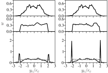
Figure 3: Profile of density distribution $w(y_{c})$ as a function of $y_{c}/r_{c}$ for microwave polarization parallel (left panels) and perpendicular (right panels) to the walls. Here we have no microwave at top panels, $\epsilon=0.1$, $j=1.7$ at middle panels, $\epsilon=0.1$, $j=2.4$ at bottom panels. In all panels we have noise amplitude $\alpha_{i}=0.01$ as in Fig. 2, dashed curves in bottom panels are obtained with $\alpha_{i}=0.05$. Simulations are done with 500 trajectories, other parameters are the same as in Fig. 2. Data for model (W1).

The dependence of density $w$ on $y_{c}$ and $j$ are shown in Fig. 2 for two polarizations of microwave field. The data show that orbits from a bulk can be captured in edge vicinity for a long time giving an increase of density in a vicinity of edge. This capture is significant around resonance values $j\approx j_{r}$. This is confirmed by a direct comparison of density profiles in Fig. 3 at $j=1.7\approx 2-1/4$ and $j=2.4\approx 2+1/4$. In the later case we have a large density peak due to trajectories trapped in a resonance (see Fig. 1) where they are synchronized with a microwave field. An increase of noise amplitude $\alpha_{i}$ gives a significant reduction of the amplitude of these resonant peaks (Fig. 3 bottom panels). The increase of density is more pronounced for polarization perpendicular to the wall in agreement with data shown in Fig.2 of adcdls .

We also performed numerical simulations using Eq. (1) with a smooth wall modeled by a potential $V_{w}(y)=\kappa y^{2}/2$. For large values $\kappa/\omega_{c}$ (e.g. $\kappa/\omega_{c}=10$) we find the Poincaré sections to be rather similar to those shown in Fig. 1 that gives a similar structure of electron density as in Figs. 2,3. A finite wall rigidity can produce a certain shift of optimal capture conditions appearing as a result of additional correction to a cyclotron period due to a part of orbit inside the wall.

The data presented in this Section show that electrons from the bulk part of the sample can be captured for a long time in edge vicinity thereby increasing the electron density near the edge. This effect is very similar to the accumulation of electrons on the edges of the electron cloud under ZRS conditions that was reported for surface electrons on Helium in adc . However we have to emphasize that the confinement potential for surface electrons is very different from the hard wall potential assumed in our simulations, as a consequence our results cannot be applied directly to this case. It is possible that the formation of ballistic channels on the edge of the sample combined with the redistribution of the electrons density can effectively short the bulk contribution and induce directly a vanishing $R_{xx}$. However, it is also important to understand how a scattering on impurities inside the bulk is affected by a microwave radiation. We study this question in next Sections.

III Scattering on a single disk

It should be noted that resistivity properties of a regular lattice of disk antidots in 2DEG had been studied experimentally weiss ; kvon and theoretically geisel1 ; geisel2 . But effects of microwave field were not considered till present.

In our studies we model an impurity as a rigid disk of fixed radius $r_{d}=v_{F}/\omega$ keeping $\omega=const$ and changing $\omega_{c}=B$. In a magnetic field a cyclotron radius moves in a free space only due to a static dc-electric field $E_{dc}$. We fix the direction of $E_{dc}$ along $x-$axis and measure its strength by a dimensionless parameter $\epsilon_{s}=E_{dc}/(\omega v_{F})$. Even in absence of a microwave field a motion in a vicinity of disk in crossed static electric and magnetic fields of moderate strength is not so simple. The studies presented in berglund and aliktrap show that dynamics in disk vicinity is described by a symplectic disk map which is rather similar to the map (3). It is characterized by a chaos parameter $\epsilon_{d}=2\pi v_{d}/(r_{d}\omega_{c})$ where $v_{d}=v_{F}E_{dc}/B$ is the drift velocity; $\epsilon_{d}$ gives an amplitude of change of radial velocity at collision. Orbits from a vicinity of disk can escape for $\epsilon_{d}>0.45$ berglund .

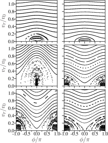
Figure 4: Poincaré section for Hamiltonian dynamics in a disk vicinity in presence of radial microwave field. Left column panels: $j=7/4,2,9/4$ at $\epsilon=0.04$ (from top to bottom); right column panels: $j=7/4,13/4,9/4$ at $\epsilon=0.02$. Here the integral of orbital momentum is $\ell_{0}/v_{F}r_{d}=v_{0}/v_{F}=1$, trajectories start from disk with fixed tangent velocity component $v_{0}=1$. Data for model (DR1).

We start our analysis from the construction of the Poincaré section in presence of microwave field at zero static field. To have a case with one and half degrees of freedom we start from a model case when a microwave field is directed only along radius from a disk center. The dynamics is described by Eq. (1) with a dimensionless microwave amplitude $\epsilon$. The dynamical evolution is obtained numerically by the Runge-Kutta method. At first we consider a case without dissipation and noise. Due to radial force direction the orbital momentum is an additional integral of motion (as $p_{x}=y_{c}$ for the wall case) and thus we have again 3/2 degrees of freedom. We call this disk model with radial microwave field as model (DR1).

The Poincaré sections at the moments of collisions with disk are shown in Fig. 4, 5 for model (DR1). Here, $v_{r}$ is the radial component of electron velocity and $\phi$ is a microwave phase both taken at the moment of collision with disk. We see that the phase space structure remains approximately the same when $j$ is increased by unity (compare $j=9/4,13/4$ panels in Fig. 4). This happens for orbits only slightly touching the disk (small $v_{r}$) since the microwave phase change during a cyclotron period is shifted by an integer amount of $2\pi$ (in a first approximation at $r_{d}\ll r_{c}$). The similarity between the wall and disk cases is directly seen from Fig. 5 as well as periodicity with $j\rightarrow j+1$.

In fact in the case of disk with a radial field the dynamics can be also described by the Chirikov standard map (3) where $v_{y}$ should be understood as a radial velocity $v_{r}$ at the moment of collision. The second equation has the same form since the change of the phase between two collisions is given by the same equation but with the parameter $\rho=1+r_{c}/r_{d}$. This expression for $\rho$ is obtained from the geometry of slightly intersecting circles of radius $r_{d}$ for disk and radius $r_{c}$ for cyclotron orbit (the angle segment of cyclotron circle is $\Delta\varphi=2v_{r}/\rho$). For $r_{d}\gg r_{c}$ this expression naturally reproduces the wall case while at $r_{d}\ll r_{c}$ we have the correction term proportional to ${\bar{v}}_{y}$ going to zero that also well corresponds to the geometry of two disks. After such modification of $\rho$ we find that the resonance positions $v_{res}=\pi\rho\delta j/j$ are proportional to $\rho$. Thus the model (DR1) reduced to the map description (3) at $\rho>1$ is called model (DR2).

The expression for $v_{res}$ works rather well. Indeed, for $j=2.1$ in Fig. 5 we obtain $v_{res}=0.149$ for model (W2) and $0.463$ for model (DR2). These values are in a good agreement with numerical values $v_{res}\approx 0.15$ for model (W2) and $v_{res}\approx 0.6$ for model (DR1). In the later case the agreement is less accurate due to a larger size of nonlinear resonance. The comparison of Poincaré sections given by the Chirikov standard map (3) and the dynamics from Newton equations, shown in Fig. 5, confirms the validity of map description.

According to the well established results for the Chirikov standard map chirikov we find for models (W1), (W2) and (DR1), (DR2) the width of separatrix $\delta v$ and the corresponding resonance energy width $E_{r}=(\delta v)^{2}/2$:

$$E_{r} = 16\epsilon\omega_{c}\rho E_{F}/\omega\;;\;\rho=1+r_{c}/r_{d}\;;$$ (4)

$$v_{res} = \pi\rho\delta j/j\;;\;\delta v=4\sqrt{\epsilon\rho/j}\;;$$

$$\delta j_{\epsilon} = \delta vj/(2\pi\rho)\;;\;j=1+\omega/\omega_{c}\;,$$

where $\delta j_{\epsilon}$ is the resonance shift produced by a resonance half width $\delta v/2=v_{res}$. This relation shows that for the disk case this energy is increased by a factor $\rho$ compared to the wall case. In majority of our numerical simulations we have $\rho=1+j$.

Thus a radial field models (DR1), (DR2) represent a useful approximation to understand the properties of dynamics in a disk vicinity but a real situation corresponds to a linear microwave polarization and the Poincaré section analysis should be modified to understand the dynamics in this case.

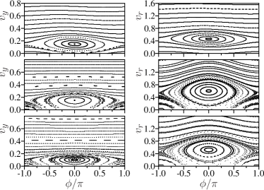
Figure 5: Poincaré sections for wall model (W1) (left) and disk model with radial electric field (DR1) (right) at $\epsilon=0.01$ and $j=2.1$ (top, middle) and $j=3.1$ (bottom). Top panels are obtained from the Chirikov standard map (3) at $\rho=1$ (left top panel), corresponding to the wall model (W2), and at $\rho=1+j=3.1$ (right top panel), corresponding to the disk model (DR2). Middle and bottom panels are obtained from solution of Newton equations (1) for wall (left) and disk (right). Other parameters are as in Fig. 1 and Fig. 4, $v_{y}$ and $v_{r}$ are expressed in units of $v_{F}$. There is no dissipation and no noise.

Due to that we start to analyze the scattering problem on a disk in presence of weak static field $\epsilon_{s}$ and microwave field $\epsilon$ using Eq. (1). For the scattering problem we find more simple to have dissipation to work only at the time moments of electron collisions with disk: at such time moments the radial component of electron velocity is reduced by a factor $v_{r}\rightarrow v_{r}/(1+\gamma_{d})$, the reduction is done only if the kinetic energy of electron is larger than the Fermi energy. Such a dissipation can be induced by phonon excitations inside the antidot disk. We fix geometry directing dc-field along $x-$axis and microwave along $y-$axis. The noise is modeled in the same way as above in Eq. (1). We call this system disk model (D1).

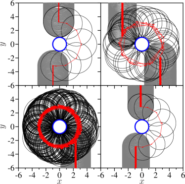
Figure 6: (Color online) Scattering of electron cyclotron trajectory on a disk scatterer (blue/black circle) in model (D1). Top left panel shows the case in absence of microwave, $\epsilon=0$, $j=9/4$. Top right panel: temporary captured path at $\epsilon=0.04$, $j=9/4$. Bottom left panel: path captured forever at $\epsilon=0.04$, $j=9/4$. Bottom right panel: no capture at $\epsilon=0.04$, $j=2$. The trajectory part colliding with disk is shown by black curve, its part before and after collisions is shown in gray. The red (light gray) points and curves show the trajectory of cyclotron center. Here the dissipation parameter is $\gamma_{d}/\omega=0.01$; the static electric field is directed along $x-$axis and $\epsilon_{s}=0.001$; microwave field is directed along $y-$axis. There is no noise here. Coordinates $x,y$ are expressed in units of $r_{d}$. Data for model (D1).

Examples of electron cyclotron trajectories scattering on disk are shown in Fig. 6. In absence of microwave field a trajectory escapes from disk rather rapidly. A similar situation appears at $j=2$ and microwave field with $\epsilon=0.04$. In contrast for $j=9/4$ and $\epsilon=0.04$ a trajectory can be captured for a long time or even forever depending on initial impact parameter.

For some impact parameters a trajectory can be captured for a very long time $t_{c}$, in certain cases in absence of noise we have $t_{c}=\infty$. At such long capture times the collisions with disk become synchronized with the phase $\phi$ of microwave field at the moment of collisions. This is directly illustrated in Fig. 7 where we show the angle $\theta$ of a collision point on disk, counted from $x-$axis, in dependence on $\phi$. Indeed, the dependence $\theta$ on $\phi$ forms a smooth curve corresponding to synchronization of two phases. At the same time the radial velocity at collisions $v_{r}$ moves along some smooth invariant curve $v_{r}(\phi)$ in the phase space $(v_{r},\phi)$. However, to make a correct comparison with the radial field models (DR1), (DR2) we should take into account that the cyclotron circle rotates around disk so that we should draw the Poincaré section in the rotational phase $\phi^{\prime}=\phi-\theta$. In this representation we see the appearance of the resonance (see right column of Fig. 7) that is similar to those seen in Figs. 4, 5 for the radial field models.

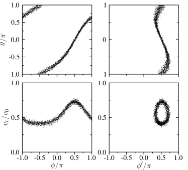
Figure 7: Synchronization between disk collision angle $\theta$ and microwave phase $\phi$. Left column: Dependence of angle $\theta$ of collision point on disk, counted from $x-$axis, and radial velocity $v_{r}$, taken at collision, on microwave phase $\phi$. Right column: Same as in left column with $\phi^{\prime}=\phi-\theta$. Here $j=2.25$, $\epsilon=0.04$, $\epsilon_{s}=0.001$, $\gamma_{d}/\omega=0.01$, $v_{0}=v_{F}$, there is no noise; points are shown for times $10^{4}/\omega<t<10^{5}/\omega$, the capture time of this orbit is $t_{c}>10^{5}/\omega$. Data for model (D1).

A more direct correspondence between radial field models (DR1), (DR2) and the model (D1) with a linearly polarized microwave field is well seen from the Poincaré sections shown in the rotation frame of phase $\phi^{\prime}=\phi-\theta$ in Fig. 8. In this frame we see directly the resonance at $j=2.1,2.25$ being very similar to the wall case and the radial field model. However, the positions of resonance at $v_{r}=v_{res}$ are different from those in Fig. 5. Of course in the rotation frame the orbital momentum is only approximately conserved that gives a broadening of invariant curves in Fig. 8.

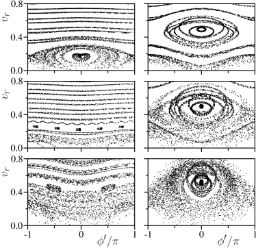
Figure 8: Poincaré sections in phase plane $(v_{r},\phi^{\prime})$ with $\phi^{\prime}=\phi-\theta$ for $j=2.1$, $\epsilon=0.01$ (left top); $j=2.25$, $\epsilon=0.01$ (right top); $j=2.75$, $\epsilon=0.02$ (left middle); $j=2.25$, $\epsilon=0.02$ (right middle); $j=2.75$, $\epsilon=0.04$ (left bottom); $j=2.25$, $\epsilon=0.04$ (right bottom); $v_{r}$ is expressed in units of $v_{F}$. Data for model (D1), no noise no dissipation.

We explain this as follows. For the linear polarized field of model (D1) the radial component of microwave field is proportional to $\epsilon_{r}\sim\epsilon\sin\theta\cos\omega t\sim 0.5\epsilon\sin(\omega t-\theta)$ where we kept only slow frequency component of radial field (the neglected term with $\sin(\omega t+\theta)$ gives resonant values $v_{res}>v_{F}$). The radial field $\epsilon_{r}$ gives kicks to the radial velocity component at collisions with disk similar to the case of model (DR2) described by Eq. (3): ${\bar{v}_{r}}=v_{r}+0.5\epsilon\sin\phi^{\prime}$, ${\bar{\phi}^{\prime}}=\phi^{\prime}+(2\pi j-2{\bar{v}_{r}}j/\rho)-2{\bar{v}_{r}(\rho-1)/\rho}$. Here we use the radial field component phase $\phi^{\prime}=\omega t-\theta$ at a moment of collision with disk (the tangent component does not change $v_{r}$ and can be neglected). The phase variation ${\bar{\phi}^{\prime}}-\phi^{\prime}$ has the first term $2\pi j-2{\bar{v}_{r}}j/\rho$ being the same as for the radial field model (DR2), and an additional term related to rotation around disk with $-\Delta\theta=-2{\bar{v}_{r}}(\rho-1)/\rho$ which comes from geometry. Indeed, the segment angles of intersections of circles $r_{d}$ and $r_{c}$ are: for disk radius $r_{d}$ it is $\Delta\theta=2{\bar{v}_{r}}(\rho-1)/\rho$ and for cyclotron radius $r_{c}$ it is $\Delta\varphi=2{\bar{v}_{r}}/\rho$. Thus, their ratio is $\Delta\theta/\Delta\varphi=r_{c}/r_{d}$ in agreement with the geometrical scaling. This result can be obtained from the expression for $\Delta\varphi$ by interchange of two disks that gives the above expression for $\Delta\theta$ (at $r_{d}=r_{c}$ both shifts $\Delta\varphi=2{\bar{v}_{r}}/\rho$ and $\Delta\theta=2{\bar{v}_{r}}(\rho-1)/\rho$ are equal).

Thus again the dynamical description is reduced down to the Chirikov standard map with slightly modified parameters giving us for the model (D1) the chaos parameter $K=2\epsilon(j+\rho-1)/\rho$ being usually smaller than unity, resonance position $v_{res}$, resonance width $\delta v$ and the resonance energy width $E_{r}=(\delta v)^{2}/2$:

$$E_{r} = 8\epsilon\rho E_{F}/(\rho+j-1);\;\rho=1+r_{c}/r_{d}\;;$$ (5)

$$v_{res} = \pi\rho\delta j/(j+\rho-1);\;\delta v=4\sqrt{\epsilon\rho/(2(j+\rho-1))};$$

$$\delta j_{\epsilon} = \delta v(\rho+j-1)/(2\pi\rho);\;j=\omega/\omega_{c}\;,$$

where $\delta j_{\epsilon}$ is a shift of resonance produced by a finite separatrix half width $\delta v/2$. For our numerical simulations we have $\rho=1+j$ with $v_{res}=\pi(j+1)\delta j/(2j)$, $\delta v=2\sqrt{\epsilon(j+1)/j}$ and $\delta j_{\epsilon}=(2/\pi)\sqrt{\epsilon j/(j+1)}$.

At $\rho=j+1$ Eq. (5) gives the values $v_{res}=0.232$ at $j=2.1$ while the numerical data of Fig. 8 give $v_{res}\approx 0.2$, and we have at $j=2.25$ the theory value $v_{res}=0.567$ being in a good agreement with the numerical value $v_{res}\approx 0.5$ of Fig. 8. For $j=2.75$ we have the resonance position at $v_{r}<0$ corresponding to the bulk and thus the resonance is absent. The resonance width in Fig. 8 at $j=2.25$, $\epsilon=0.01$ can be estimated as $\delta v\approx 0.3$ that is in a satisfactory agreement with the theoretical value $\delta v=0.24$ from (5). We remind that in model (D1) we have only approximate conservation of orbital momentum that gives a broadening of invariant curves and makes determination of the resonance width less accurate. In spite of this broadening we see that the resonance description by the Chirikov standard map works rather well.

In Fig. 9 we show the dependence of average capture time $t_{c}$ on $j$ in the model (D1). The averaging is done over $N_{s}=500$ trajectories scattered on disk at all such impact parameters that cyclotron orbit can touch the disk. Here, we show the ratio $t_{c}/t_{c}(0)$ where $t_{c}(0)$ is an average capture time in absence of microwave. According to our numerical data we have approximate dependence $\omega t_{c}(0)\approx 3/\sqrt{\epsilon_{s}}$ corresponding to a period of nonlinear oscillations in a disk map description discussed in berglund ; aliktrap .

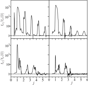
Figure 9: Dependence of rescaled capture time $t_{c}/t_{c}(0)$ on $j$ at $\epsilon=0.04$ shown at various static fields: $\epsilon_{s}=2.5\cdot 10^{-4}$ (top left), $10^{-3}$ (top right), $8\cdot 10^{-3}$ (bottom left), $0.016$ (bottom right). Here $\gamma_{d}/\omega=0.01$, there is no noise. Data for model (D1).

The data of Fig. 9 show a clear periodic dependence of capture time $t_{c}$ on $j$ corresponding to the periodicity variation of Poincaré section with $j$ (see Figs. 4, 5. 8). This structure is especially well visible at weak static fields. With an increase of $\epsilon_{s}$ this structure is suppressed. Indeed, at large $\epsilon_{s}$ even without microwave field the trajectories can escape from disk as it discussed in berglund ; aliktrap and microwave field does not affect the scattering in this regime.

The distributions of capture times are shown in Fig. 10. We clearly see that at resonant values of $j$ a microwave field leads to appearance of long capture times. For example, we have the probability to be captured for $t_{c}>180/\omega$ being $W=0.46$ at $j=2.25$ while at $j=2$ we have $W=0$(left panel in Fig. 10); and we have $W=0.38$ at $j=2.37$ while at $j=1.9$ we have $W<3\cdot 10^{-4}$ (right panel in Fig. 10). These data confirm much stronger capture at certain resonant values of $j$.

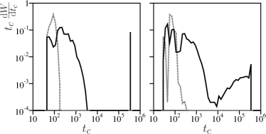
Figure 10: Differential probability distribution $t_{c}dW/dt_{c}$ of capture times $t_{c}$ for parameters of Fig. 9. Left panel: $j=2$ (dashed curve for minimum of capturing probability) and $j=2.25$ (full curve at maximum of capturing probability) at $\epsilon_{s}=0.001$. Right panel: similar cases at $j=1.9$ (dashed curve) and $j=2.37$ (full curve) at $\epsilon_{s}=0.002$. Data are obtained with $N_{s}=5\cdot 10^{4}$ trajectories started at different impact parameters and running up to time $t=3\cdot 10^{5}/\omega$. Here $t_{c}$ is expressed in units of $1/\omega$. Data for model (D1).

The data of Figs. 9, 10 show that the scattering process on disk is strongly modified by a microwave field. However, to determine the conductivity properties of a sample we need to know what is an average displacement $\Delta x$ along static field after a scattering on a single disk. Indeed, in our model a dissipation is present only during collisions with disk while in a free space between disks the dynamics is integrable and Hamiltonian. Hence during such a free space motion there is no displacement along the static field (the dissipative part of conductivity or resistivity appears only due to dissipation on disk). The dependence of $\Delta x$ on $j$ is shown in Fig. 11. In absence of microwave field at $\epsilon=0$ we find $\Delta x\propto 1/j\propto B$ that corresponds to a simple estimate $\Delta x\propto\omega_{c}\gamma_{d}$. The numerical data show that $\Delta x$ is practically independent of $\epsilon_{s}$ and that $\Delta x=0$ in absence of dissipation at $\gamma_{d}=0$. In presence of microwave field we see that the displacement along the static field has strong periodic oscillations with $j$. The striking feature of Fig. 11 is the appearance of windows of zero displacement $\Delta x\approx 0$ at resonance values $j_{r}=9/4,13/4,17/4...$. We discuss how this scattering on a single disk modifies the resistance of a sample with large number of disks in next Section.

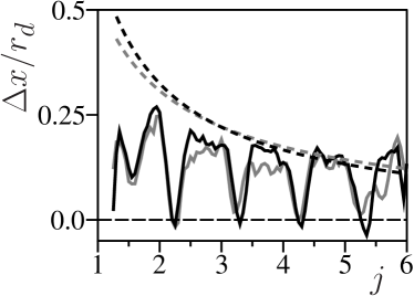
Figure 11: Average shift $\Delta x$ along static field after scattering on a single disk shown as a function of $j$ at various amplitudes of static and microwave fields: $\epsilon_{s}=0.0005$, $\epsilon=0$ (gray dashed curve); $\epsilon_{s}=0.001$, $\epsilon=0$ (black dashed curve); $\epsilon_{s}=0.0005$, $\epsilon=0.04$ (gray full curve); $\epsilon_{s}=0.001$, $\epsilon=0.04$ (black full curve). The data are obtained by averaging over $N_{s}=5\cdot 10^{3}$ scattered trajectories with random impact parameters; here $\gamma_{d}/\omega=0.01$, noise amplitude $\alpha_{i}=0.005$. Data for model (D1).

IV Resistance of samples with many disks

To determine a resistance of a sample with many disks we use the following scattering disk model. The scattering on a single disk in a static electric field $\epsilon_{s}$ is computed as it is described in the previous Section with a random impact parameter inside the collision cross section $\sigma_{d}=2(r_{c}+r_{d})$. After that a trajectory evolves along $y$-axis according to the exact solution of Hamiltonian Eq. (1) (no dissipation and no noise) up to a collision with next disk which is taken randomly on a distance between $2(r_{c}+r_{d})$ and $2\ell_{e}$ where $\ell_{e}=1/(\sigma_{d}n_{d})$ is a mean free path along $y-$axis and $n_{d}$ is a two-dimensional density of disks (of course $\ell_{e}\gg 2(r_{c}+r_{d})$). In a vicinity of disk the dynamical evolution is obtained by Runge-Kutta solution of dynamical equations as it was the case in previous Section. We use low disk density with $n_{d}r_{d}^{2}\sim 1/100$. The collision with disk is done with a random impact parameter in the $x-$axis of disk vicinity: the impact parameter is taken randomly in the interval $[-(r_{c}+r_{d}),(r_{c}+r_{d})]$ around disk center. Noise acts only when a center of cyclotron radius of trajectory is on a distance $r<r_{d}+r_{c}$ from disk center so that a collision with disk is possible. After scattering on a disk a free propagation follows up to next collision with disk.

Along such a trajectory we compute the average displacement $\delta x$ and $\delta y$ after a time interval $\delta t$. In this way the number of collisions with disks is $N_{col}\approx\delta y/\ell_{e}$ and a total displacement in $x-$axis is $\delta x\approx N_{c}\Delta x$ where $\Delta x$ is an average displacement on one disk discussed in previous Section. We compute the global displacements $\delta x,\delta y$ on a time interval $\delta t=10^{6}/\omega$ averaging data over 200 trajectories. We call this system model (D2).

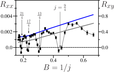
Figure 12: Dependence of resistivity $R_{xx}$ and $R_{xy}$ on magnetic field $B=1/j$ (resistivity is expressed in arbitrary numerical units). Blue and gray curves show respectively $R_{xx}$ and $R_{xy}$ in absence of microwave field. Black curve with points show $R_{xx}$ dependence of $B$ at microwave field $\epsilon=0.04$ (here $B$ is expressed in units of $1/\omega=const$). Here $\epsilon_{s}=0.001$, $\gamma_{d}/\omega=0.01$, noise amplitude $\alpha_{i}=0.005$, $\tau_{i}=1/\omega$. Resonant values $j_{r}$ are shown by arrows; bars show statistical errors for $R_{xx}$. Data are obtained by averaging over 200 trajectories propagating up to time $t=10^{6}/\omega$. Data for model (D2).

Then the current components are equal to $j_{x}=\delta x/\delta t$, $j_{y}=\delta y/\delta t$ and conductivity components are $\sigma_{xx}=j_{x}/E_{dc}$, $\sigma_{xy}=j_{y}/E_{dc}$ (the current is computed per one electron). We work in the regime of weak dc-field where $j_{x},j_{y}$ scales linearly with $E_{dc}$. The current $j_{y}$ is determined by the drift velocity $v_{d}=E_{dc}/B\ll v_{F}$. Since the mean free path is large compared to disk size $\ell_{e}\gg r_{c}\geq r_{d}$ we have an approximate relation $\sigma_{xy}\approx 1/B$, $\sigma_{xx}\approx\Delta x/B\ell_{e}\approx\sigma_{xy}\Delta x/\ell_{e}$. As in 2DEG experiments mani2002 ; zudov2003 we have in our simulations $\sigma_{xy}/\sigma_{xx}=R_{xy}/R_{xx}\sim 100$ (see Fig. 12). The resistivity is obtained by the usual inversion of conductivity tensor with $R_{xx}=\sigma_{xx}/(\sigma^{2}_{xx}+\sigma^{2}_{xy})\approx\sigma_{xx}/\sigma^{2}_{xy}$, $R_{xy}=\sigma_{xy}/(\sigma^{2}_{xx}+\sigma^{2}_{xy})\approx 1/\sigma_{xy}$. The dependence of $R_{xx}$, $R_{xy}$, expressed in arbitrary numerical units, on magnetic field $B=\omega/j=1/j$ is shown in Fig. 12.

In absence of microwave field we find $R_{xy}\propto B$ and $R_{xy}/R_{xx}\approx 200$ similar to experiments mani2002 ; zudov2003 . For small noise amplitude (e.g. $\alpha_{i}=0.005$) we have $R_{xx}$ growing linearly with $B$ (see Fig. 12) but at larger amplitudes (e.g. $\alpha_{i}=0.02$) its increase with $B$ becomes practically flat showing only $30\%$ increase in a give range of $B$ variation.

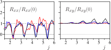
Figure 13: (Color online) Rescaled values of resistivity $R_{xx}$ (left panel) and $R_{xy}$ (right panel) as function of $j=\omega/\omega_{c}$ at various noise amplitudes $\alpha_{i}=0.005$ (black curve), $0.01$ (blue/dark curve), $0.02$ (red/gray curve). Here $\epsilon=0.04$, $\epsilon_{s}=0.001$, other parameters are as in Fig. 12. Curves are drown though numerical points obtained with a step $\Delta j=0.1$. Data for model (D2).

In presence of microwave field the dependence of $R_{xx}$ on $B$ is characterized by periodic oscillations with minimal $R_{xx}$ values being close to zero at resonant values of $j=j_{r}$ well visible in Fig. 12. The dependence of $R_{xx}$, $R_{xy}$ rescaled to their values $R_{xx}(0)$, $R_{xy}(0)$ in absence of microwave field are shown in Fig. 13 at various amplitudes of noise and fixed $\epsilon$, and in Fig. 14 at various $\epsilon$ and fixed noise amplitude $\alpha_{i}$. We see that increase on noise leads to an increase of minimal values of $R_{xx}$ at resonant values $j_{r}$. In a similar way a decrease of microwave power leads to increase of minimal values of $R_{xx}$ at $j_{r}$. At the same time the Hall resistance $R_{xy}$ is only weakly affected by microwave radiation as it also happens in ZRS experiments.

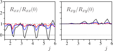
Figure 14: (Color online) Same as in Fig. 13 at various microwave amplitudes $\epsilon=0.01$ (red/gray curve), $0.02$ (blue/dark curve), $0.04$ (black curve); amplitude of noise is fixed at $\alpha_{i}=0.005$. Data for model (D2).

These results are in a qualitative agreement with the ZRS experiments. On the basis of our numerical studies we attribute the appearance of approximately zero resistance at $j_{r}$ values in our bulk model of disk scatterers to long capture times of orbits in disk vicinity at these $j_{r}$ values (see Fig. 9). During this time $t_{c}$ noise gives fluctuations of collisional phase $\theta$ and due to that a cyclotron circle escapes from disk practically at random displacement $\Delta x$ that after averaging gives average $\Delta x=0$. Since resistivity is determined by the average value of $\Delta x$ this leads to appearance of ZRS. We note that this mechanism is different from the one of edge transport stabilization discussed here and in adcdls . However, both mechanisms are related to a long capture times near edge or near disk that happens due to synchronization of cyclotron phase with microwave field phase and capture inside the nonlinear resonance.

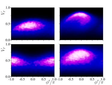
Figure 15: (Color online) Phase space $(v_{r},\phi^{\prime})$ of trajectories at the moment of collisions with disks for parameters of Fig. 14 at $\epsilon=0.04$: $j=2.1$ (top left), $j=2.25$ (top right), $j=2.75$ (bottom left), $j=3.25$ (bottom right). Here $\phi^{\prime}=\phi-\theta$ where $\phi=\omega t$ is a microwave phase at the moments of collisions with disk and $\theta$ is the angle on disk at collision moment, counted from $x$-axis (same as in Figs. 7, 8). Data are obtained from $500$ trajectories iterated up to time $t=10^{6}/\omega$. Density of points is shown by color with black at zero and white at maximum density. The average number of collisions per disk per trajectory is $N_{col}=12.4$, $25.9$, $9.5$, $15.5$ respectively for $j=2.1$, $2.25$, $2.75$, $3.75$. Data are obtained for model (D2).

To illustrate the capture inside the resonance we present the distributions of trajectories from Fig. 14 shown in the phase space plane $(v_{r},\phi^{\prime})$ at the moments of collisions with disks in Fig. 15. This is similar to the Poincaré sections of Fig. 8 however, now we consider the real case of diffusion and scattering on many disks in the model (D2) with noise and dissipation. We see that for $j=2.25$ orbits are captured in a vicinity of the center of nonlinear resonance at $\phi^{\prime}\approx 0$ well seen in Fig. 8. For $j=2.1$ we have a density maximum located at smaller values of $v_{res}$ and $\phi^{\prime}\approx 0$ even if there is a certain shift of $v_{res}$ produced by a significant resonance width at $\epsilon=0.04$. At $j=2.75$ we have a density maximum at $\phi^{\prime}\approx\pm\pi$ corresponding to an unstable fixed point of separatrix. The total number of collision points $N_{col}$ in this case is by a factor $2.5$ smaller than in the case of stable fixed point at $j=2.25$. A similar situation is seen in the case of wall model (W1) (see Fig.1d,f in adcdls ) even if there the ratio between number of captured points was significantly larger. The results of Fig. 15 show that in the ZRS phase the collisions with disk indeed create synchronization of cyclotron and microwave phases and capture of trajectories inside the nonlinear resonance.

However, there are also some distinctions between bulk disk model (D2) and experimental observations. The first one is that there are minima for $R_{xx}/R_{xx}(0)$ but there are no peaks which are well visible around integer $j$ values in ZRS experiments mani2002 ; zudov2003 ,dmitrievrmp and numerical simulations of transport along the edge adcdls . The second one is appearance of small negative values of $R_{xx}$ at $j_{r}$ values.

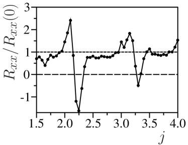
Figure 16: Dependence of $R_{xx}/R_{xx}(0)$ on $j$ in the disk model with dissipation at disk collisions at rate $\gamma_{d}/\omega=0.01$ and dissipation in disk vicinity with rate $\gamma_{0}/\omega=0.02$; a disk roughness gives additional angle rotations with amplitude $\alpha_{d}=0.1$ (see text); the amplitude of noise in disk vicinity is $\alpha_{i}=0.001$. Here we have $\epsilon=0.04$, $\epsilon_{s}=0.001$; 51 numerical points in $j$ are connected by lines to adapt an eye. Data are obtained by averaging over 100 trajectories propagating up to time $t=10^{6}/\omega$. Data for model (D3).

We attribute the absence of peaks to a specific dissipation mechanism which takes place only at disk collisions. It is rather convenient to run long trajectories using exact solution for free propagation between disks. Indeed, in this scheme there is no dissipation during this free space propagation and thus these parts of trajectories have no displacement along static field. We also tested a dissipation model with additional $\gamma(v)=\gamma_{0}(|v/v_{F}|^{2}-1)$ for $|v|>v_{F}$ and $\gamma(v)=0$ for $|v|\leq v_{F}$. This dissipation works only in a disk vicinity when the distance between disk center and cyclotron center is smaller than $r_{d}+r_{c}$. The dissipation $\gamma_{d}$ on disk remains unchanged. We also added a certain roughness of disk surface modeled as an additional random angle rotation of velocity vector in the range $\pm\alpha_{d}$, done at the moment of collision with disk. We call this system disk model (D3). The results for the resistivity ratio $R_{xx}/R_{xx}(0)$ are shown in Fig. 16. They show an appearance of clear peaks of $R_{xx}/R_{xx}(0)$ in presence of such additional dissipation in vicinity of integer $j$. There is also a small shift of minima from integer plus $1/4$ to integer plus $0.4-0.5$.

The second point of distinctions from ZRS experiments is a small negative value of $R_{xx}$ at resonant $j$ values. It is relatively small for disk model (D2) (see Figs. 13, 14) and it becomes more pronounced for disk model (D3) (see Fig. 16). It is possible that a scattering on disk in presence of dissipation, noise, static and microwave field gives a negative displacement $\Delta x$ which generates such negative $R_{xx}$ values. We expect that in the limit of static field going to zero this effect disappears. Indeed, the negative values become smaller at smaller $\epsilon_{s}$ according to data of Fig. 11 but unfortunately the small $\epsilon_{s}$ limit is also very difficult to investigate numerically.

We consider that at this stage of the theory the presence of negatives values for $R_{xx}$ does not constitute a critical disagreement. The escape parameters for electrons that have been captured on an impurity for a time long enough to make many rotations around it, are likely to strongly depend on the model for the electron impurity interaction and further theoretical work on a more microscopic model is needed. In general a zero average displacement along the field direction seems natural for a smooth distribution of trapping times with a characteristic time scale much larger than the rotation time around the impurity (this assumption does not seem to hold for our model, see for example the sharp features on Fig. 10). Finally in Section VII we propose a slightly different mechanism by which the combination of trapping on impurities investigated here and electron-electron interactions can lead to ZRS.

V Physical scales of ZRS effect

The ZRS experiments mani2002 ; zudov2003 show that the resistance $R_{xx}$ in the ZRS minima scales according to Arrehenius law $R_{xx}\propto\exp(-T_{0}/T)$ with a certain energy scale dependent on a strength of microwave field. In typical experimental conditions one finds very large $T_{0}\approx 20K$ at $j_{r}=5/4$ (see e.g. Fig.3 in zudov2003 ). These data also indicate the dependence $T_{0}\propto 1/j_{r}\propto B$. This energy scale $k_{B}T_{0}$ is very large being only by a factor $7$ smaller than the Fermi energy $E_{F}/k_{B}\approx 150K$. At the same time the amplitude of microwave field is rather weak corresponding to $\epsilon\approx 0.003$ at field of $1V/cm$ or ten times larger at $10V/cm$ (unfortunately it is not known what is an amplitude of microwave field acting on an electron).

As in adcdls we argue that the Arrehenius scale is determined by the energy resonance width (4) with $T_{0}=E_{r}/k_{B}$. Indeed, the resonance forms an energy barrier for a particle trapped inside the resonance by dissipative effects being analogous to a wash-board potential. An escape from this potential well requires to overcome the energy $E_{r}$ leading to the Arrehenius law for $R_{xx}$ dependence on temperature. Assuming the case of the wall with $\rho=1$ we obtain at $E=3V/cm$ the activation temperature $T_{0}\approx 23K$ being is a satisfactory agreement with the experimental observations. The theoretical relation (4) also reproduces the experimental dependence $T_{0}\propto 1/j_{r}$ at $\rho=1$. In his relation $T_{0}\propto\epsilon\propto E$ being confirmed by the numerical simulations presented in adcdls . This dependence is in a satisfactory agreement with the power dependence found in experiments mani2002 . In other samples one finds that the dependence $T_{0}\propto\epsilon^{2}$ works in a better way. We think that higher terms in a nonlinear resonance can be responsible for scaling $T_{0}\propto\epsilon^{2}$ being different from the relation (4). Also a finite rigidity of the wall or disk scatterers can be responsible for appearance of higher power of $\epsilon$.

The energy scale $E_{r}$ on disks is enhanced by a factor $\rho=1+r_{c}/r_{d}$ for the case of radial field (4). However, we showed that for a linear polarization the scale $E_{r}$ is given by Eq.(5) and thus there is no enhancement at large $\rho$. Indeed, we performed direct simulations at parameters of Fig. 14 with the reduced value of disk radius by a factor 2. The numerical data give approximately the same traces $R_{xx}/R_{xx}(0)$ vs. $j$ at $\epsilon=0.01,0.02,0.04$ without visible signs of deeper minima at small $\epsilon$. This confirms the theoretical expressions (5). In any case, for small values $r_{d}\ll r_{c}$ one should analyze the quantum scattering problem which is significantly more complex compared to the classical case. We may assume that in a quantum case one should replace $r_{d}$ by a magnetic length $a_{B}\approx r_{c}/\sqrt{\nu}\propto\sqrt{B}$. In such a case we are getting $\rho=1+\sqrt{\nu}\approx 9$ that gives $T_{0}\approx 8K$ at $j\approx 2.25$ and microwave amplitude $E\approx 3V/cm$. However, in this case we obtain the scale $T_{0}$ being practically independent of $j$ which differs from experimental data. In any case in experiments the size of impurities is small compared to $r_{c}$ and a quantum treatment is required to reproduce the correct picture for $R_{xx}$ dependence on parameters in the ZRS phase.

Another point is related to the positions of ZRS minima on $j$ axis. We remind that that for the wall model the resonance is located at $v_{res}=\pi\delta j/j$ (4) and that the separatrix width is $\delta v=4\sqrt{\epsilon/j}$. The capture of trajectories from the bulk is most efficient when a half width of separatrix touch the border of bulk at $v_{r}=0$ with $v_{res}=\delta v/2$ that gives the expression $\delta j_{\epsilon}=2\sqrt{\epsilon j}/\pi$ for the wall case. At $\epsilon=0.06$, $j=2.25$ this gives $\delta j_{\epsilon}=0.22$ being in a good agreement with the numerical data $\delta j\approx 1/4$ for $R_{xx}$ dependence on $j$ (see Figs.2,3 in adcdls with a visible tendency of $\delta j$ growth with $j$). For the data presented here in Fig. 14 for the disk case at $\epsilon=0.04$, $\rho=1+j$, $j=2.25$ we obtain from (5) $\delta j_{\epsilon}=0.11$ that is slightly less than the numerical value $\delta j\approx 0.25$ for minima location. We attribute this difference to an approximate nature of expression for the resonance width at relatively strong microwave fields. We also note that in experiments an additional contribution to the value of $\delta j$ can appear due to a finite rigidity of disk and wall potentials.

VI Theoretical predictions for ZRS experiments

The theoretical models presented here and in adcdls reproduce main experimental features of ZRS experiments mani2002 ; zudov2003 ,dmitrievrmp . However, it would be useful to have some additional theoretical predictions which can be tested experimentally. A certain characteristic feature of both wall and disk models is appearance of nonlinear resonance. For example, according to the wall model (W2) described by Eq. (3) the dynamics inside the resonance is very similar to dynamics of a pendulum. The frequency of phase oscillations inside the resonance is $\Omega_{ph}=\sqrt{K}=2\sqrt{\epsilon\omega/\omega_{c}}=2\sqrt{\epsilon j}\ll 1$ chirikov . Here the frequency is expressed in number of map iterations and since the time between collisions is approximately $2\pi/\omega_{c}$ we obtain the physical frequency $\Omega_{r}$ of these resonant oscillations being $\Omega_{r}/\omega=\Omega_{ph}\omega_{c}/(2\pi\omega)=\sqrt{\epsilon\omega_{c}/\omega}/\pi$. At $\epsilon\sim 0.02$ this frequency is significantly smaller than the driving microwave frequency. The dynamics inside the resonance should be very sensitive to perturbations at frequency $\omega_{1}\approx\Omega_{r}$ that gives:

$$\omega_{1}/\omega=\sqrt{\epsilon\omega_{c}/\omega}\;/\pi\;\;.$$ (6)

To check this theoretical expectation we study numerically the effect of additional microwave driving with dimensional amplitude $\epsilon_{1}$ ($\epsilon_{1}\ll\epsilon$) and frequency $\omega_{1}$. We use the wall model (W2) based on the Chirikov standard map described here and in adcdls . As for the additional driving frequency we have $\epsilon_{1}=|E_{1}|/(\omega_{1}v_{F})$ where $E_{1}$ is the field strength of microwave frequency $\omega_{1}$, we assume that both main and additional fields are collinear and perpendicular to the wall. In presence of second frequency the map (3) takes the form:

$${\bar{v}_{y}} = v_{y}+2\epsilon\sin\phi+2\epsilon_{1}\sin(\omega_{1}\phi/\omega)+I_{cc},\;$$ (7)

$${\bar{\phi}} = \phi+2(\pi-{\bar{v}_{y}})\omega_{/}\omega_{c}\;.$$

The only modification appears in the first equation since now the change of velocity at collision depends on both fields; the second equation remains the same as in (3). As in the model (W2) the term $I_{cc}$ describes the effects of dissipation with rate $\gamma_{c}$ and noise with amplitude $\alpha$ of random velocity angle rotations. We call this system model (W3).

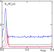
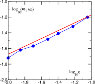
Figure 17: (Color online) Left panel: Dependence of rescaled resistance $R_{xx}/R^{\epsilon}_{xx}(0)$ on frequency ratio $\omega_{1}/\omega$ in model (W3) described by the map (7). Here, the test driving at frequency $\omega_{1}$ has fixed amplitude $\epsilon_{1}=0.007$; the main microwave driving is located in the ZRS phase at $j=\omega/\omega_{c}=2.25$, and its amplitude takes values $\epsilon=0.02$ (blue curve), $0.03$ (green curve), $0.04$ (magenta curve), $0.06$ (red curve) (these curves follow from top to bottom at $\omega_{1}/\omega=0.2$). The values of $R_{xx}$ are computed at fixed $\epsilon_{1}=0.007$ and corresponding $\epsilon$; the values of $R^{\epsilon}_{xx}(0)$ are computed at $\epsilon_{1}=0$ and $\epsilon=0.02$. The data are obtained at noise amplitude $\alpha=0.02$ and dissipation $\gamma_{c}=0.01$; averaging is done over 2000 trajectories for 5000 iterations of map (7). Right panel: Dependence of peak position $\omega_{1}/\omega$ on main microwave driving amplitude $\epsilon$ obtained from data of left panel at $\epsilon_{1}=0.007$ and additional data at $\epsilon_{1}=0.003$ (blue points), the theory dependence (6) at $\omega/\omega_{c}=2.25$ is shown by the straight red line. Data for model (W3).

In the model (W3) the resistance $R_{xx}$ is computed numerically in the same way as in the model (W2) described in adcdls : the displacement along the edge between collisions is $\delta x=2v_{y}/\omega_{c}$; it determines the total displacement $\Delta x$ along the edge during the total computation time $\Delta t\sim 10^{4}/\omega$; then $R_{xx}\propto 1/D_{x}=\Delta t/(\Delta x)^{2}$ where $D_{x}$ is an effective diffusion rate along the edge. To see the effect of additional weak test driving $\epsilon_{1}$ at frequency $\omega_{1}$ we place the system in the ZRS phase at $j=\omega/\omega_{c}=2.25$ and measure the variation of rescaled resistance $R_{xx}/R^{\epsilon}_{xx}(0)$. Here $R_{xx}$ is the resistance in presence of both microwave fields $\epsilon$ and $\epsilon_{1}$ while $R^{\epsilon}_{xx}(0)$ is the resistance at $\epsilon_{1}=0$ and a certain fixed $\epsilon$. The dependence of $R_{xx}/R^{\epsilon}_{xx}(0)$ on the frequency ratio is shown in Fig. 17 at left panel. The main feature of this data is appearance of peak at low frequency ratio $\omega_{1}/\omega<0.1$. In the range $0.1<\omega_{1}/\omega<0.4$ the testing field $\epsilon_{1}$ is nonresonant and does not affect $R_{xx}$ however at $\omega_{1}/\omega<0.1$ it becomes resonant to the pendulum oscillations in the wall vicinity and hence strongly modifies $R_{xx}$ value. The dependence of this resonance ratio $\omega_{1}/\omega$ on amplitude of main driving field $\epsilon$ is shown in right panel of Fig. 17. The numerical data are in a good agreement with the above theoretical expression (6).

The theoretical dependence (6) allows to check the synchronization theory of edge state stabilization. It also allows to measure the strength of main microwave driving force acting on an electron that still remains an experimental challenge. The experimental testing of relation (6) requires to work with good ZRS samples which have every low resistance in ZRS minima since this makes the effect of testing field $\omega_{1}$ to be more visible. We note that the recent experiments in a low frequency regime $\omega/\omega_{c}\ll 1$ alikcam demonstrate that $R_{xx}$ is sensitive to low frequency driving. The expression (6) is written for the case when $R_{xx}$ is mainly determined by a transport along edges. If the dominant contribution is given by bulk disk scatterers then a certain numerical coefficient $A$ should be introduced in the right part of the expression. According to the data of Fig. 8 and Eqs. (5) we estimate $A\approx 0.5$ (the separatrix width is smaller for the disk case compared to the wall case at the same $\epsilon$).

Another interesting experimental possibility of our theory verification is to take a Hall bar of high mobility 2DEG sample and put on it antidots with regular or disordered distribution (it is important to have no direct collision-less path for a cyclotron radius in crossed dc-electric and magnetic fields) with a low density of antidot disks $n_{d}r_{d}^{2}\ll 1$ (as in our numerical studies) so that an average distance between antidots is larger than the cyclotron radius $r_{c}$. The regular antidot lattices have been already realized experimentally weiss ; kvon . The effect of microwave field on electron transport in a regular lattice has been studied in the frame of ratchet transport in asymmetric lattices portal . Even a case of symmetric circular antidots has been studied in portal but the lattice was regular and no special attention was paid to analysis of resistivity at ZRS resonant regime with $j\approx j_{r}$. We think that the experimental condition of portal can be relatively easy modified to observe the ZRS effect on disk scatterers discussed here.

VII Discussion

Above we presented theoretical and numerical results which in our opinion explain the appearance of microwave induced ZRS in high mobility samples. The synchronization theory of ZRS proposed in adcdls and extended here is based on a clear physical picture: high harmonics $\omega_{/}\omega_{c}=j>1$ are generated by collisions with sharp edge boundary or isolated impurities which are modeled here by specular disks. The ZRS phases appear in a vicinity of resonant values $j_{r}\approx 1+1/4,\;2+1/4,\;...$ . At these $j_{r}$ values the cyclotron phase of electron motion becomes synchronized with the microwave phase due to dissipative processes present in the system.

For trajectories at the edge vicinity this synchronization gives stabilization of propagation along edge channels that creates an exponential drop of resistivity contribution of these channels with decreasing amplitude of thermal noise and increasing amplitude of microwave field. The contribution to resistivity from trajectories in the bulk is analyzed in the frame of scattering on many well separated disk impurities. Here again the synchronization of cyclotron phase with the microwave phase takes place approximately at the same resonant $j_{r}$ values. At these $j_{r}$ values the synchronization leads to long time capture of trajectories in disk vicinity. During this long time an initial cyclotron phase is washed out by noisy fluctuations and many rotations around disk and thus an electron escapes from a disk with an average zero displacement along the applied dc-field even if dynamics in disk vicinity is dissipative. This provides the main mechanism of suppression of dissipative resistivity contribution from isolated impurities in the bulk. As a result the contribution of bulk to dissipative conductivity $\sigma_{xx}$ is suppressed, as it was assumed in adcdls , and the main contribution to current is given by electron propagation along edge states stabilized by a microwave field.

As we showed above the resonance width or resonance energy scale $E_{r}$ are approximately the same for the disk and wall cases (see Eqs. (4, 5)). We note that for the disk case the energy $E_{r}$ is not sensitive to the disk radius as soon as it is significantly smaller than the cyclotron radius. Thus we expect that at $j_{r}$ values the conductivity $\sigma_{xx}$ in the bulk is suppressed by a microwave field and at these fields the current is flowing essentially along stabilized edge states. In the case of Corbino geometry we have radial conductivity $\sigma_{rr}$ which is determined by the bulk scattering and now the minima of $\sigma_{rr}$ are located at $j_{r}$ values (see e.g Figs. 12, 13,14 where $R_{xx}\propto\sigma_{xx}\sim\sigma_{rr}$). The ZRS experiments performed in the Corbino geometry give minima of $\sigma_{rr}$ at these $j_{r}$ values (see e.g. zudovcorbino ; bykovcorbino ) being in agreement with the synchronization theory.

It is interesting to note that the nonlinear dynamics in vicinity of edge and disk impurity is well described by the Chirikov standard map chirikov . The map description explains the location of resonances at integer values of $j$ with an additional shift $\delta j\approx 1/4$ produced by a finite separatrix width of nonlinear resonance. A finite rigidity of wall or disk potential can give a modification of this shift $\delta j$.

Our results show that the ZRS phases at $j_{r}$ appear only at weak noise corresponding to high mobility samples. Strong noise destroys synchronization and trajectories are no more captured at edge or disk vicinity. We also note that internal sample potentials with significant gradients act like a strong local dc-field which destroys stability regions around disk impurities or near edge. Due to that the ZRS effect exists only in high mobility samples. The resistance at ZRS minima drops significantly with the growth of microwave field strength since it increases the amplitude of nonlinear resonance which captures the synchronized trajectories.

The synchronization theory of ZRS is based on classical dynamics of noninteracting electrons. It is possible that electron-electron interaction effects can also suppress the contribution to resistivity from neutral short range range scatterers (interface roughness, adatoms,…). Indeed, long capture times can increase the electron density around these short ranged impurities transforming them into long range charged scatters that the other electrons can circumvent by adiabatically following the long range component of the disorder potential thereby avoiding a scattering event. However, the theoretical description of this short-ranged impurity cloaking mechanism for the ZRS effect remains a serious challenge.

Another important step remains the development of a quantum synchronization theory for ZRS. Even if in experiments the Landau level is relatively high $\nu\sim 60$, there are only about ten Landau levels inside a nonlinear resonance adcdls and quantum effects should play a significant role. The general theoretical studies show that the phenomenon of quantum synchronization persists at small effective values of Planck constant $\hbar_{eff}$ but it becomes destroyed by quantum fluctuations at certain large values of $\hbar_{eff}$ qsync .

The importance of quantum ZRS theory is also related to a short range nature of the impurities considered here, typically on a scale of a few nanometers or even less. We have modeled these impurities by disks with a radius that was only several times (in fact $j$ times) smaller than the cyclotron radius which is not so close to microscopic reality. We could argue that in the quantum case a nanometer sized impurity would act effectively as an impurity of a size of quantum magnetic length $a_{B}\sim r_{c}/\sqrt{\nu}\approx r_{c}/8\sim 100nm$. This gives a ratio $r_{c}/a_{B}\sim 8$ which is comparable with the one used in our simulations with $r_{c}/r_{d}=j\sim 7$ but of course a quantum treatment of scattering on nanometer size impurity in crossed electric and magnetic and also microwave fields remains a theoretical challenge. We note that such type of scattering can be efficiently analyzed by tools of quantum chaotic scattering (see e.g. martina ; main ) and we expect that these tools will allow to make a progress in the quantum theory development of striking ZRS phenomenon.

We hope that the synchronization theory of microwave induced ZRS phenomenon described here can be tested in further ZRS experiments.

VIII Acknowledgments

This work was supported in part by ANR France PNANO project NANOTERRA; OVZ was partially supported by the Ministry of Education and Science of Russian Federation.

We dedicate this work to the memory of Boris Chirikov (06.06.1928 - 12.02.2008).

References

- (1) R.G. Mani, J.H. Smet, K. von Klitzing, V. Narayanamurti, W.B. Johnson, and V. Umansky, Nature 420, 646 (2002).
- (2) M.A. Zudov, R.R. Du, L.N. Pfeiffer, and K.W. West, Phys. Rev. Lett. 90, 046807 (2003).
- (3) S.I. Dorozhkin, JETP Lett. 77, 577 (2003)
- (4) J. H. Smet, B. Gorshunov, C. Jiang, L. Pfeiffer, K. West, V. Umansky, M. Dressel, R. Meisels, F. Kuchar, and K. von Klitzing, Phys. Rev. Lett. 95, 116804 (2005)
- (5) A.A. Bykov, A.K. Bakarov, D.R. Islamov, and A.I. Toropov, JETP Lett. 84, 391 (2006)
- (6) D. Konstantinov, and K. Kono, Phys. Rev. Lett. 105, 226801 (2010)
- (7) D.Konstantinov, A.D.Chepelianskii, and K.Kono, Jour. Phys. Soc. Japan 81, 093601 (2012)
- (8) I.A. Dmitriev, A.D. Mirlin, D.G. Polyakov, and M.A. Zudov, Rev. Mod. Phys. 84, 1709 (2012)
- (9) A.D. Chepelianskii, and D.L. Shepelyansky, Phys. Rev. B 80, 241308(R) (2009)
- (10) A. Pikovsky, M. Rosenblum, and J. Kurths, Synchronization: A Universal Concept in Nonlinear Sciences, Cambridge Univ. Press, Cambridge (2001)
-
(11)
A.D. Chepelianskii, Non linear transport in
drift-diffusion equations under magnetic field,
arXiv:1110.2033[cond-mat.mes-hall] (2011) - (12) W. G. Hoover, Time reversibility, computer simulation, and chaos, World Sci., Singapore (1999)
- (13) B.V. Chirikov, Phys. Rep. 52, 263 (1979)
- (14) A.J. Lichtenberg, and M.A. Lieberman, Regular and chaotic dynamics, Springer, Berlin (1992).
- (15) B.Chirikov, and D.Shepelyansky, Scholarpedia 3(3), 3550 (2008)
- (16) Y. Avishai, and G. Montambaux, Eur. Phys. J. B 79, 215 (2011)
- (17) F. Benvenuto, G. Casati, I. Guarneri, and D. L. Shepelyansky, Z. Phys. B Cond. Mat. 84, 159 (1991)
- (18) D. Weiss, M. L. Roukes, A. Menschig, P. Grambow, K. von Klitzing, G. Weimann, Phys. Rev. Lett. 66, 2790 (1991)
- (19) G. M. Gusev, V. T. Dolgopolov, Z. D. Kvon, A. A. Shashkin, V. M. Kudryashov, L. V. Litvin and Yu. Nastaushev, Pis’ma Zh. Eksp. Teor. Fiz. 54, 369 (1991)
- (20) R. Fleischmann, T. Geisel, and R. Ketzmerick, Phys. Rev. Lett. 68, 1367 (1992)
- (21) T. Geisel, R. Ketzmerick and O. Schedletzky, Phys. Rev. Lett. 69, 1680 (1992)
- (22) N. Berglund, A. Hansen, E. H. Hauge, and J. Piasecki, Phys. Rev. Lett. 77, 2149 (1996)
- (23) A.D. Chepelianskii, and D.L. Shepelyansky, Phys. Rev. B 63, 165310 (2001)
- (24) A.D. Chepelianskii, J. Laidet, I. Farrer, H.E. Beere, D.A. Ritchie, and H. Bouchiat, Phys. Rev. B 86, 205108 (2012)
- (25) S. Sassine, Yu. Krupko, J.-C. Portal, Z.D. Kvon, R. Murali, K.P. Martin, G. Hill, and A.D. Wieck, Phys. Rev. B 78, 045431 (2008)
- (26) C.L. Yang, M.A. Zudov, T.A. Knuuttila, R.R. Du, L.N. Pfeiffer, and K.W. West, Phys. Rev. Lett. 91, 096803 (2003)
- (27) A.A. Bykov, JETP Lett. 87, 551 (2008)
- (28) O.V. Zhirov, and D.L. Shepelyansky, Eur. Phys. J. D 38, 375 (2006)
- (29) J. Wiersig, and M. Hentschel, Phys. Rev. Lett. 100, 033901 (2008)
- (30) A. Eberspächer, J. Main, and G. Wunner, Phys. Rev. E 82, 046201 (2010)