“Ping-pong” electron transfer.
I. First reflection of the Loschmidt echo.

Abstract

Quantum dynamics of the electron wave function on one-dimensional lattice is considered. The lattice consists of $N$ equal sites and one impurity site. The impurity site differs from other sites by the on-site electron energy $E$ and the hopping integral $C$. The wave function is located on the impurity site at $t=0$. The wave packet is formed which travels along the lattice, and reflects from its end. Reflections happen many times (Loschmidt echo) and this phenomenon is considered in the second part of the paper. Analytical expressions for the wave packet front propagation at different values $E$ and $C$ are derived, and they are in excellent agreement with the numerical simulation. The obtained results can help in interpretation of recent experiments on highly efficient charge transport in synthetic olygonucleotides.

PACS numbers: 87.15.-v; 42.15.Dp

Keywords: charge transport, Loschmidt echo, wave packet, DNA

^∗The corresponding author: gvin@deom.chph.ras.ru.

I INTRODUCTION

Charge transfer (CT) is the key event in many processes in living and inorganic matter. The particular interest has been expressed after the effective charge transfer in synthetic olygonucleotides was found Aug07 ; Bar11 ; Gen10 ; Mal10 ; Gie02 . There are possibilities to synthesize the DNA analogues with the bases sequences up to dozens base pairs. For example, the double strand consisting of 100 base pairs adenosine–thymine (A-T)₁₀₀ was synthesized Sli11 . This synthetic olygonucleotide have regular structure and very effective with regard to the CT. Synthetic DNA and polypeptides can be utilized in nanobiology Gie06 ; Gao11 . They are also considered as potential molecular wires Mal07 . It is worth noting that the CT can occur as the one-step coherent process Gen11 .

Experiments on the charge transfer are usually done when donor $D$ and acceptor $A$ are attached to both sides of the molecular chain: $D-(b)_{N}-A$. The charge is transferred from donor on the chain and travels along the chain $-(b)_{N}-$ consisting of $N$ repeating DNA bases (usually adenine). The charge can be trapped by an acceptor and registered by photophysical response (fluorescence) or electrochemical reactions.

If an acceptor is absent then the charge is locked on the chain and can reflect from the end. Many reflections can happen (the phenomenon of Loschmidt echo, i.e. multiple returning to the initial state, was extensively studied in classical and quantum systems Qua06 ; Jac02 ; Cuc03 ; Pro03 ; Man06 ). V. Benderskii with colleagues investigated the analogous quantum dynamics of vibrational excitations in 1D molecular chain Ben07 ; Ben08 ; Ben11 . It worth noting that the property to form the moving wave packet is an attribute of discrete lattices. The diffusive spreading of the initially localized excitation is usually observed in continuous models.

The recurrence phenomena to the initial state are well known. This property is also typical for some dynamical systems. The Fermi-Pasta-Ulam recurrence is an example Fer55 ; Ber05 . The other example is the interaction of the isolated vibrational mode with the continuous spectrum Ovc01 .

The recurrence in the quantum systems was for the first time considered by R. Zwanzig Zwa60 for the discrete equidistante spectrum when single level is initially populated. The analysis of the Zwanzig’s problem is done in Ben07 . The same authors generalized their consideration in the next paper Ben08 . The quantum dynamics of the vibrational excitation on the one-dimensional lattice was considered in Ben11 . It was shown that if the excitation is initially localized in the lattice center, then the energy is not distributed homogeneously along the lattice but conversely it localizes and reflects from the lattice ends many times.

In the present paper we consider an analogous problem of the wave packet propagation on the lattice and multiple reflections from the lattice ends. One of the goals is an explanation of efficient charge transport in synthetic olygonucleotides.

II Setting up a problem

We consider a lattice consisting of $N$ identical sites and one impurity site at the left lattice end. The excitation is initially confined to the impurity site. An excitation can be electronic or vibronic. The electronic excitation is considered for definiteness.

The wave function amplitude on the impurity site is labelled by $a(t)$, and amplitudes on other sites $b_{i}(t)\,\,(i=1,2,\ldots,N)$. The electron can hop on the neighboring site. The electron energy on all sites except the impurity site is zero, what corresponds to the choice of the reference point for electron energy. The hopping integral $C=1$, what corresponds to the choice of energy unit. $E$ is the on-site energy of the impurity site, and $C$ – the hopping integral between the impurity site and the nearest site of the lattice. The challenge is to find how the electronic populations of all sites change in time.

The hamiltonian in the $(N+1)\times(N+1)$ matrix representation reads:

$$H=\begin{pmatrix}{\bf E}&{\bf C}&0&\cdots&0&0&0\\ {\bf C}&0&1&\cdots&0&0&0\\ 0&1&0&\cdots&0&0&0\\ \cdots&\cdots&\cdots&\cdots&\cdots&\cdots&\cdots\\ 0&0&0&\cdots&0&1&0\\ 0&0&0&\cdots&1&0&1\\ 0&0&0&\cdots&0&1&0\\ \end{pmatrix}$$ (1)

with the wave function

$$\Psi(t)=a(t),b_{1}(t),b_{2}(t),\ldots,b_{N}(t).$$ (2)

In the second quantization representation the hamiltonian is

$$H=Ea^{+}a^{-}+\sum_{i=1}^{N-1}b^{+}_{i+1}b^{-}_{i}+\sum_{i=2}^{N}b^{+}_{i-1}b^{-}_{i}+C\left(a^{+}b_{1}^{-}+b_{1}^{+}a^{-}\right)\,.$$ (3)

The dimensionless ($\hbar=1$) Schrödinger equation for the wave function has the form

$$\left\{\begin{split}i\dot{a}=&\,Ea+Cb_{1}\\ i\dot{b}_{1}=&\,b_{2}+Ca\\ i\dot{b}_{2}=&\,b_{1}+b_{3}\\ \cdots\,\,\,\,&\,\cdots\cdots\cdots\\ i\dot{b}_{N}=&\,b_{N-1}\\ \end{split}\right.$$ (4)

with the initial conditions $\left.a(t)\right|_{t=0}=1$ and $\left.b_{i}(t)\right|_{t=0}=0\,\,(i=1,2,\ldots,N)$. The formulated problem mimics the experiments on the charge transfer in synthetic DNA Bar11 .

If equations (4) are integrated numerically then the phenomenon of repeated reflections from the lattice ends is observed, i.e. Loschmidt echo or the electronic “ping-pong” (the electronic ping-pong was found experimentally Eli08 ). The result is shown in Fig. 1.

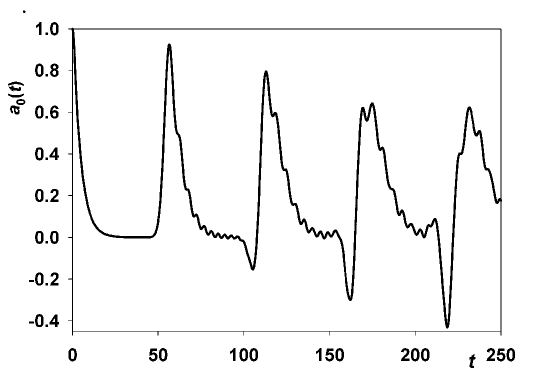
Figure 1: The dependence of the wave function amplitude $a(t)$ on the impurity site vs. time. The wave function returns many times (four times in the figure) to the impurity site with slightly decreasing amplitudes. Parameters: $E=0$, $C=\sqrt{2}$, $N=50$.

The goal of the present paper is the consideration of the wave packet propagation and its first reflection from the lattice end. This time interval corresponds to the time range $0\leq t<100$ in Fig. 1. Next part of the paper considers the multiple reflections of the wave packet.

The quantum dynamical problem of the wave packet evolution can be treated as the interaction of the impurity site with the reservoir. And it is solved using the expansion in terms of the eigenfunctions of the reservoir.

The lattice without the impurity site (reservoir) is described by the $N\times N$ tridiagonal matrix with zero leading diagonal and the unity values on the secondary diagonals. Eigenvalues $\varepsilon(k)$ and eigenfunctions $q_{i}(k)$ of this matrix are well known:

$$\varepsilon(k)=2\,\cos\left(\dfrac{\pi k}{N+1}\right);\quad q_{i}(k)=\sqrt{\dfrac{2}{N+1}}\sin\left(\dfrac{\pi k}{N+1}i\right).$$ (5)

It is more convenient to consider the problem in terms of amplitudes of modes $b(k)$ instead of amplitudes on the lattice sites $b_{i}$. These values are related by the orthogonal relationship:

$$b(k,t)\equiv\sum_{i=1}^{N}q_{i}(k)\,b_{i}(t);\quad b_{i}(t)\equiv\sum_{k=1}^{N}q_{i}(k)\,b(k,t).$$ (6)

Then the system (4) can be written in the form:

$$\left\{\begin{split}i\dot{a}(t)=&\,Ea(t)+C\sum_{k=1}^{N}q_{1}(k)\,b(k,t)\\ i\dot{b}(k,t)=&\,\varepsilon(k)\,b(k)+Ca(t)\,q_{1}(k)\\ \end{split}\right.$$ (7)

Amplitudes $b(k,t)$ in (7) are expressed through the amplitude $a(t)$:

$$b(k,t)=q_{1}(k)\exp[-i\,\varepsilon(k)\,t]\,\int_{0}^{t}a(\tau)\,\exp[i\,\varepsilon(k)\,\tau]\,{\rm d}\tau\,.$$ (8)

Substituting this expression into equation (7) for $a(t)$, one can get the integro-differential equation for the amplitude $a(t)$ on the impurity site:

$${\dot{a}(t)}=-i\,E\,a(t)-C^{2}\int_{0}^{t}B^{N}(t-t^{\prime})\,a(t^{\prime}){\rm d}\,t^{\prime},$$ (9)

where the kernel is given by the following sum:

$$B^{N}(t)=\dfrac{2}{N+1}\sum_{k=1}^{N}\sin^{2}\left(\dfrac{\pi k}{N+1}\right)\exp\left[-2\,i\,\cos\left(\dfrac{\pi k}{N+1}\right)t\right].$$ (10)

Our primary goal is the solution of (9) for the amplitude $a(t)$ on the impurity site.

III The decay of the initial state $a(t=0)=1$ in the semi-infinite lattice

Initially we consider the decay kinetics of the initial state $\left.a(t)\right|_{t=0}=1$ in the semi-infinite lattice ($N\to\infty$). The amplitude on the impurity site is labelled by $a_{0}(t)$ in this case. In the expression (10) for the kernel $B^{N}(t)$ we use the limit $N\to\infty$. The limiting value (at $N\to\infty$) of the expression for $B^{N}(t)$ is labelled by $B_{0}(t)$.

The sum (10) in the limit $N\to\infty$ is modified to the integral Gra07 :

$$B_{0}(t)\equiv\lim B^{N}(t)\left.\right|_{N\to\infty}=J_{0}(2t)+J_{2}(2t).$$ (11)

And in this limit we have the following equation for the amplitude $a_{0}(t)$:

$$\dot{a}_{0}(t)=-iEa_{0}(t)-C^{2}\int_{0}^{t}B_{0}(t-t^{\prime})\,a_{0}(t^{\prime})\,{\rm d}t^{\prime}.$$ (12)

This equation can be solved using the Laplace transformation:

$$a_{0}(p)=\dfrac{1}{p+iE+C^{2}\,B_{0}(p)}\,,$$ (13)

where the Laplace transform $B_{0}(p)$ of the function $B_{0}(t)$ Gra07 :

$$B_{0}(p)=\dfrac{1}{2}\,\left(\sqrt{p^{2}+4}-p\right).$$ (14)

The amplitude $a_{0}(t)$ can be obtained by the inverse Laplace transformation:

$$a_{0}(t)=\int\limits_{d-i\infty}^{d+i\infty}\dfrac{\exp(p\,t)}{p+iE+C^{2}\dfrac{1}{2}\left(\sqrt{p^{2}+4}-p\right)}\,{\rm d}p,\quad d>0.$$ (15)

The obtained form of the expression for $a_{0}(t)$ is very inconvenient for the analysis and numerical computations (integral with the upper infinite limit converges very slowly). The convenient form this integral obtains if the integration contour is closed around the cut $[-2i,+2i]$, and the square root $\sqrt{p^{2}+4}$ should be rewritten in the form: $\sqrt{p^{2}+4}=-i\,\sqrt{ip+2}\,\sqrt{ip-2}$. The integration contour can be closed if amplitude $a_{0}(p)$ has no poles. Assuming that poles are absent, close the integration contour and summing the integrals along both banks of the cut, one gets the following expression for amplitude $a_{0}(t)$:

$$a_{0}(t)=\dfrac{1}{\pi}\int_{-2}^{+2}{\rm d}\omega\exp(i\omega t)\,{\rm Im}\left[\omega+E-\dfrac{C^{2}}{2}\left(\omega+i\sqrt{4-\omega^{2}}\right)\right]^{-1}.$$ (16)

Few special cases can be noted, when the integral (16) is calculated explicitly and the amplitude $a_{0}(t)$ is expressed through the Bessel functions Gra07 :

$$\begin{split}a_{0}(t)=&J_{0}(2t);\qquad\qquad\qquad(E=0,\,\,C=\sqrt{2})\\ a_{0}(t)=&J_{0}(2t)+J_{2}(2t);\qquad(E=0,\,\,C=1)\\ a_{0}(t)=&J_{0}(2t)-iJ_{1}(2t);\qquad(E=1,\,\,C=1)\\ \end{split}$$ (17)

An integro-differential equation for the amplitude $a_{0}(t)$ is derived in Appendix A, and its solution is obtained as a series in terms of the Bessel functions. These series have simple form in few particular cases when $E=0$ or $C=1$.

Fig. 2 shows the dependence of the amplitude $a_{0}(t)$ vs. time at $E=0$ and at different values of the hopping integral $C^{2}$. The comparison with the accurate result is also shown (“accurate” result $\equiv$ numerical integration of equations (4)).

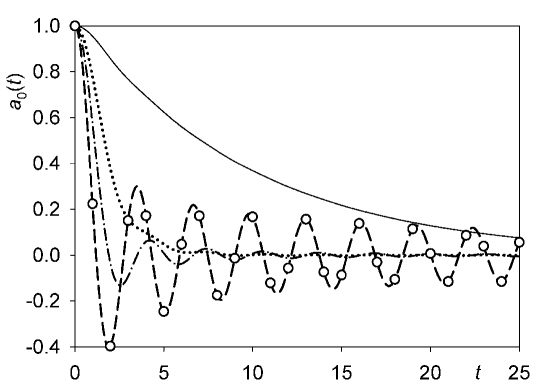
Figure 2: The dependence of the amplitude $a_{0}(t)$, calculated according to (16), vs. time at $E=0$. Solid line: $C^{2}=0.1$; dotted line: $C^{2}=0.5$; dash-dotted line: $C^{2}=1$; dashed line: $C^{2}=2$. Empty circles – accurate result for $C^{2}=2$, when $a_{0}(t)=J_{0}(2t)$.

The dependence of the amplitude vs. time in (16) can be estimated by the Fermi’s golden rule, when the perturbation approximation by the small parameter $C^{2}$ is used, and when an exponential decay is valid:

$$a_{0}(t)\approx\exp\left(-C^{2}\sqrt{4-E^{2}}\,t\right).$$ (18)

More accurate expression for the amplitude $a_{0}(t)$ at small values of parameter $C$ is given in Appendix B.

Now we consider the case when amplitude $a_{0}(p)$ has poles. An analysis shows that one pole exists in the region $E>2-C^{2}$, and two poles – when $E<C^{2}-2$. There are no poles in the region $|E|<2-C^{2}$ ($C^{2}<2$). Fig. 3 shows number of poles vs. values of parameters $E$ and $C$.

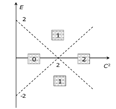
Figure 3: Number of poles of the integrand of function (16) in regions divided by dashed lines.

As an example we consider the case of one pole in the region $E>2-C^{2}$ ($C^{2}<2$). The pole is located at the point $p=-i\varepsilon$ ($\varepsilon>2$). The relation between parameters $E$ and $C$ follows from (15):

$$E=\varepsilon\left(1-\dfrac{C^{2}}{2}\right)+\dfrac{C^{2}}{2}\,\sqrt{\varepsilon^{2}-4}.$$ (19)

The contribution from the pole $\Delta a_{0}$ is equal to

$$\Delta a_{0}(t)=\dfrac{\exp(-i\varepsilon t)}{1+\dfrac{C^{2}}{2}\left(\dfrac{\varepsilon}{\sqrt{\varepsilon^{2}-4}}-1\right)}.$$ (20)

The overall amplitude is the sum of the main term (16) and the pole contribution (20). The dependence of amplitude vs. time when one pole exists, is shown in Fig. 4. In this case the amplitude on the impurity site does not decrease to zero and $\left.a_{0}(t)\right|_{t\to\infty}=0{.}75$.

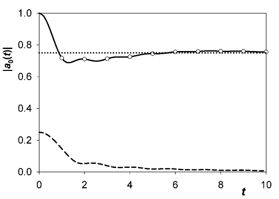
Figure 4: The dependence of amplitude $a_{0}(t)$ vs. time in the presence of one pole. Dashed line – contribution to amplitude from the integral summand (16); dots – modulus of the pole summand (equal to 0.75) (20); empty circles – numerical result. Parameters: $E=2,\,\,C=1\,\,(\varepsilon=2.5)$.

In Appendix C it is shown that if $|E|>2-C^{2}$ ($C^{2}<2$), then there exists the bounded state localized at the lattice end. The value $\varepsilon$ (see (19)) is the energy of this localized state and its contribution to the amplitude $a_{0}(t)$ coincides with the contribution from the pole summand. Note also that the integral term (16) is the contribution to the amplitude from the continuous spectrum which lies in the range $[-2,\,2]$. The fraction of the initial state is trapped by this localized state and the smaller part of the initial state goes out to the reservoir. The effect of returning to the initial state also decreases. This case (existence of a pole) seams to be less interesting and we consider only an absence of the localized state when the integral (16) is the accurate result for the amplitude $a_{0}(t)$.

Such a detailed analysis of the amplitude $a_{0}(t)$ decay in the infinite lattice is done by two reasons. First, the decay kinetics in the infinite lattice coincides with the kinetic in the finite lattice consisting of $N$ sites in the time range $0\leq t\lesssim N$. Second, as will be shown in the second part of the paper, the overall amplitude in the finite lattice can be represented as a sum of partial amplitudes, first of which is just the amplitude $a_{0}(t)$.

IV Wave packet propagation on the lattice

The dynamics of the wave function on the lattice, i.e. spatiotemporal evolution of amplitudes $b_{j}(t)$, is considered in this section. Initially the expected spreading of the wave packet is observed. But then amplitudes on the sites with larger numbers increase. And when the amplitude $a(t)$ becomes small, the wave function forms the well defined wave packet with the sharp forward front. This behavior is shown in Fig. 5.

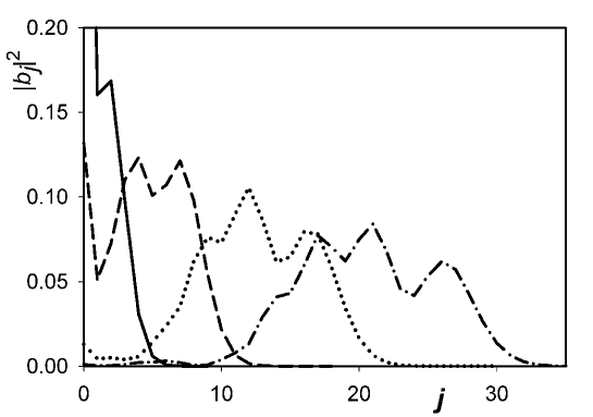
Figure 5: Spatiotemporal evolution of the wave packet. Solid line: $t=2$; dashed line: $t=5$; dotted line: $t=10$; dash-dotted line: $t=15$. Site $j=0$ corresponds to $|a_{0}(t)|^{2}$. Parameters: $E=1$, $C^{2}=0.5$. $N=100$.

An expression for amplitudes $b_{j}(t)$ is obtained by the substitution expression (8) for the mode amplitudes $b(k,t)$ into expression (6). Then one gets the following equation

$$b_{j}(t)=-\dfrac{i2C}{N+1}\sum_{k=1}^{N}\sin\left(\dfrac{\pi k}{N+1}\right)\sin\left(\dfrac{\pi k}{N+1}j\right)\exp[-i\varepsilon(k)t]\int_{0}^{t}\exp[-i\varepsilon(k)\tau]a(\tau){\rm d}\tau.$$ (21)

Initially we consider the case of semi-infinite lattice ($N\to\infty$). Changing the summation in (21) by integration and replacing $a(t)$ by $a_{0}(t)$, the following expression can be obtained:

$$b_{j}(t)=-\dfrac{i2C}{\pi}\int_{0}^{\pi}{\rm d}k\sin(k)\sin(kj)\exp[-i\varepsilon(k)t]\int_{0}^{t}\exp[-i\varepsilon(k)\tau]a(\tau){\rm d}\tau\,,$$ (22)

where $\varepsilon(k)=2\cos(k)$.

Consider the case when time $t$ is large and amplitude $a_{0}(t)$ is very small, $|a_{0}(t)|\ll 1$. Then the upper limit in integration over time in (22) is infinity. The obtained integral is the Laplace transformation $a_{0}(p)$ taken at $p=-i\varepsilon(k)$. As a result we have:

$$b_{j}(t)=-\dfrac{2C}{\pi}\int_{0}^{\pi}{\rm d}k\dfrac{\sin(k)\sin(kj)\exp[-2it\cos(k)]}{E-2\cos(k)+C^{2}\exp(-ik)},\qquad|a_{0}(t)|\ll 1\,.$$ (23)

Expression (23) can formally be generalized on the negative values of index $j$. Aiming this in mind, the multiplier $\sin(kj)$ is represented as the difference of two exponents. Then expression (23) describes the superposition of two wave packets freely travelling to the left and to the right in the infinite (to both sides) lattice. Every wave packet is normalized to unity. Consider separately the wave packet propagating to the right. Label this wave packet by $b_{j}^{\rm inf}$:

$$b_{j}^{\rm inf}(t)=-\dfrac{iC}{\pi}\int_{0}^{\pi}{\rm d}k\dfrac{\sin(k)\exp\left\{-i[kj+2\cos(k)\,t]\right\}}{E-2\cos(k)+C^{2}\exp(-ik)},\qquad-\infty<j<+\infty\,.$$ (24)

The considered impulse $b_{j}$ (in the region $j>0$) is the following difference:

$$b_{j}(t)=b_{j}^{\rm inf}(t)-b_{-j}^{\rm inf}(t).$$ (25)

The addend $b_{-j}^{\rm inf}(t)$ is the “tail” of the impulse $b_{j}(t)$, and it is small at large times, e.g. $\sim 1/t$. Then it can be assumed that $b_{j}^{\rm inf}(t)$ is a good approximation for $b_{j}(t)$. The snapshots of the impulse at different time points are shown in Fig. 6. One can see that the constrain by the impulse $b_{j}^{\rm inf}(t)$ is a very good approximation.

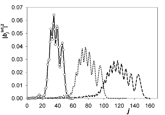
Figure 6: Snapshots of the impulse in semi-infinite lattice at $t=25$ (solid line); $t=50$ (dotted line); $t=75$ (dashed line). Calculations according to (24). Empty circles – numerical integration of (4). The coincidence of the numerical and analytical results is also excellent for $t=50$ and $t=75$ (mean square error (MSE) $\lesssim 10^{-4}$).

Expression $b_{j}^{\rm inf}(t)$ (see (24)) is a reliable approximation for the propagating impulse on the time interval $t\lesssim N/2$ for the finite but comparatively long lattices. Moreover, as will be demonstrated below, this expression allows to describe the impulse reflection from the lattice end on the time interval $N/2\lesssim t\lesssim N$.

Lets analyze the expression (24) at large times. As the integrand is the fast oscillating function, the stationary phase method can be applied. If $j<t/2$, then two stationary points exist which are determined by the equality $\sin(k)=j/2t$. Then the following expression can be obtained:

$$\widetilde{b}_{j}(t)\approx\dfrac{-iC}{\sqrt{\pi t\cos(k_{0})}}\left[f(\pi-k_{0})\exp(i\pi/4)+f(\pi-k)\exp(-i\pi/4)\right],\quad k_{0}\equiv\arcsin(j/2t).$$ (26)

Here $f(k)$ is the integrand in expression (24).

Fig. 7 compares the expression (26), obtained by the stationary phase method, with the accurate answer.

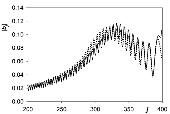
Figure 7: The impulse front at $t=200$ $(E=1,\,C^{2}=2,\,N=500)$. Dotted line – numerical result, solid line – the asymptotic expansion(28).

If $j\approx 2t$, then both stationary points lie close to the point $k=\pi/2$ and the stationary phase method gives false results (if both points coincide then the answer diverges). Lets consider this region $(j\approx 2t)$ in more details. In this case the expression for amplitudes (24) can be simplified:

$$\widetilde{b}_{j}(t)\approx-\dfrac{iC\exp(-0.5\pi j)}{\pi(2-C^{2})}\int_{-\infty}^{\infty}{\rm d}x\dfrac{\exp\left[i\left(\dfrac{j-2t}{\sqrt[3]{t}}x+\dfrac{1}{3}x^{3}\right)\right]}{z-x},\quad z(t)\equiv\dfrac{(E-iC^{2})\sqrt[3]{t}}{2-C^{2}}.$$ (27)

If $|z(t)|\gg 1$ (what is valid for $t\gg 1$), then the asymptotic expansion of (26) can be rewritten as a series in Airy functions:

$$\widetilde{b}_{j}(t)\approx-\dfrac{2iC}{z(t)(2-C^{2})}\left[{\rm Ai}(\widetilde{j})+\dfrac{1}{iz(t)}{\rm Ai}^{\prime}(\widetilde{j})-\dfrac{1}{z^{2}(t)}{\rm Ai}^{\prime\prime}(\widetilde{j})+\ldots\right],\quad\widetilde{j}=\dfrac{j-2t}{\sqrt[3]{t}}.$$ (28)

Thereafter an approximate expression for the impulse front can be written. Using the asymptotics of the Airy function, one can notice that the dominant term, describing the impulse front, has the form:

$$\widetilde{b}_{j}(t)\approx-\dfrac{1}{z(t)}\exp\left[-\dfrac{2}{3}\left(\dfrac{j-2t}{\sqrt[3]{t}}\right)^{2/3}\right].$$ (29)

Fig. 8 shows the comparison of the asymptotic expansion (28) with the numerical answer.

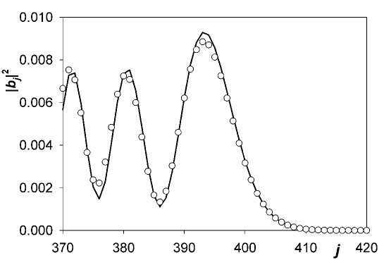
Figure 8: The impulse front at $t=200$ $(E=1,C^{2}=2)$. Empty circles – numerical result, solid line – asymptotic expansion (28). MSE $\lesssim 10^{-4}$.

Expression (29) allows to describe qualitatively the form of the impulse front. The dependence on the lattice number $j$ is defined by the argument $(j-2t)/\sqrt[3]{t}$ (see (27)). From (28) one can see that the impulse front slowly spreads: its width increases $\propto\sqrt[3]{t}$ and amplitude decreases $\propto 1/\sqrt[3]{t}$. The front velocity is 2 – maximal possible group velocity. The front has the sharp profile. Thus, if the finite lattice is considered, then until the front achieves the lattice end, its propagation is the same as in infinite lattice. Front of the impulse achieves the lattice end at $t\approx N/2$. After that the impulse reflects from the lattice end and the front moves back to the impurity site.

Now we consider the impulse reflection. Lets assume that the lattice is long enough. Then amplitude $a(t)$ is negligible and impulse is totally formed. The impulse front moving with the velocity $v=2$, reaches the lattice end at $t\approx N/2$. After reflection it moves with the same velocity $v=2$ in the opposite direction. And at $t\approx N$ the impulse reaches the impurity site on the left end. Amplitude $a(t)$ starts to increase. We consider the impulse evolution at time range $t<N$, when amplitude $a(t)$ is small and when it coincides with the amplitude $a_{0}(t)$ — amplitude in the infinite lattice.

V Impulse reflection

To derive an expression for the reflected impulse we come back to the expression (21) for amplitudes $b_{j}(t)$. We assume that the time is large such that amplitude $a(t)$ is small. Then the upper limit in integration over time is infinity and the substitution $a(t)\to a_{0}(t)$ is made. As earlier, the obtained integral can be represented as the Laplace transformation of $a_{0}(p)$ at $p=-i\varepsilon(k)$. Then the following expression can be deduced:

$$b_{j}(t)=-\dfrac{2C}{N+1}\sum_{k=1}^{N}\sin(\widetilde{k})\sin(\widetilde{k}j)\exp[-2it\cos(\widetilde{k})]\left(E-2\cos(\widetilde{k})+C^{2}\exp(-i\widetilde{k})\right)^{-1},$$ (30)

where $\widetilde{k}=\pi k/(N+1)$.

This expression can be modified using the Poisson summation formula:

$$\sum_{k=-\infty}^{k=\infty}f(k)=\sum_{m=-\infty}^{m=\infty}\int\limits_{-\infty}^{\infty}f(x)\,\exp(-2\pi imx)\,{\rm d}x$$ (31)

and the function $f(k)$ differs from 0 on the interval $[0,N+1]$. After substitution of variables $\pi x/(N+1)\equiv y$, the following series can be obtained:

$$b_{j}(t)=-\dfrac{2C}{\pi}\sum_{m=-\infty}^{m=\infty}\int\limits_{0}^{\pi}\dfrac{\sin y\sin(jy)\exp\left\{-i[2t\cos y+2my(N+1)]\right\}}{E-2\cos y+C^{2}\exp(-iy)}{\rm d}y.$$ (32)

This series can be represented as a sum of two series, expressed through the amplitude $b_{j}^{\rm inf}$ — the amplitude in the infinite lattice at large time (see (24)):

$$b_{j}(t)=\sum_{m=-\infty}^{m=\infty}b_{j+2m(N+1)}^{\rm inf}(t)-\sum_{m=-\infty}^{m=\infty}b_{-j+2m(N+1)}^{\rm inf}(t)$$ (33)

For the separating terms, which are significant in the considered time range $(1\ll t<N)$, the expression (24) should be analyzed and the terms, where the phase has the stationary point, should be found. From the first sum the single term with $m=0$ is left which describes the incident impulse $b_{j}^{\rm inf}$. From the second sum – the term with $m=1$, i.e. $b_{-j+2(N+1)}^{\rm inf}$ describing the reflected impulse. Thus, if $t<N$ then the impulse can be represented as the sum of two terms:

$$b_{j}(t)=b_{j}^{\rm inf}(t)-b_{-j+2(N+1)}^{\rm inf}(t).$$ (34)

Fig. 9 shows the impulse reflection calculated according to (34).

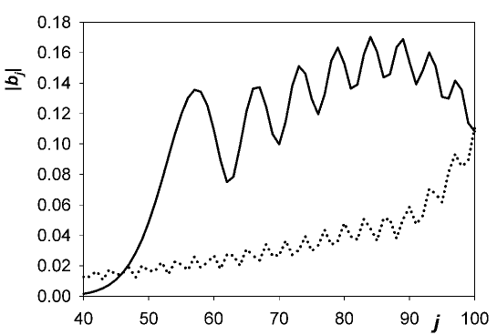
Figure 9: Reflection of the impulse from the lattice end ($N=100$). Time $t=75$. Parameters: $E=1,\,\,C^{2}=0.5$. Computation according to (26). Solid line – reflected impulse, dotted line – tail of the incident impulse. At $t=75$ the impulse front, moving with $v=2$, passed $\approx 150$ lattice sites: 100 sites before reflection and 50 sites after reflection. An excellent agreement with numerical simulation is observed (MSE $<10^{-4}$, numerical data are not shown).

At $t\approx N$ the impulse front returns to the lattice beginning and starts to interact with the impurity site. Amplitude $a(t)$ increases. Our approximation concerning the smallness of $a(t)$ becomes invalid. The system returns to the initial state. This process will be analyzed in the next paper.

VI Conclusions

The electronic impulse propagates starting from the impurity site at the lattice end. If the electronic excitation is entirely located on the impurity site then, depending on the impurity site parameters, few scenarios of the wave function dynamics are realized. One, most common case, is the formation of impulse and its propagation along the lattice. The impulse moves with the maximal group velocity $v=2$ and has the steep forward front. After reaching the opposite lattice end, the impulse reflects and moves in the opposite direction. This process repeats many times. The other scenario is realized, if the parameters of the impurity site are such that the bounded state is formed. Then the wave function is partially trapped by this bounded state.

The analytical expressions describing the impulse dynamics coincide with the accurate numerical simulation.

The problem of the electronic excitation travelling along the lattice, being formulated in a rather simple form, can be relevant to recent experiments on the charge transfer in synthetic olygonucleotides and polypeptides.

At one time it seemed that the polaron mechanism can adequately explain the charge transport in biomacromolecules. But there exists at least to weak points in this approach. First, – polaron formation. After a charge is transferred to the chain it should be more or less localized for some time to allow the polaron formation. Otherwise the wave function spreads very fast along the lattice because of very small hopping time. Second problem, – how the polaron can get an initial momentum necessary for the coherent movement. The discussed mechanism of quantum dynamical charge transfer allows to exclude this difficulties in explaining the high efficient CT over long distances: the electronic wave packet, responsible for the charge transport, spontaneously forms and moves.

Appendix A

An expression for amplitude (see (15)) can be rewritten in the following form:

$$a_{0}(t)=\dfrac{C^{2}}{2\pi}\int\limits_{-2}^{2}{\rm d}\omega\dfrac{\sqrt{4-\omega^{2}}\exp(i\omega t)}{(\omega+E)\,(\omega+E-\omega C^{2})+C^{4}}.$$ (35)

This expression can be rearranged to the differential equation by time. It can be done if the denominator of the integrand is represented as the differential operator with the replacement $\omega\to-i{\rm d}/{\rm d}t$. Then the action of this differential operator on both sides of equation (35) eliminates the denominator. The resulting integral is expressed through the Bessel functions. As a result the following differential equation is obtained:

$$(1-C^{2})\,\ddot{a}_{0}+iE(2-C^{2})\,\dot{a}_{0}-(C^{4}+E^{2})\,a_{0}=-C^{2}\left[J_{0}(2t)+J_{2}(2t)\right].$$ (36)

Hence the inhomogeneous linear differential equation of the second order is derived. Initial conditions for this equation are: $a_{0}(t=0)=1$ and ${\rm d}a_{0}/{\rm d}t|_{t=0}=-iE$ (the second condition follows from equation (12)).

The solution of this equation can be formally written as the integral over time. But this integral is difficult to evaluate analytically and numerical calculation is more complex compared to the original expression (13).

Nevertheless we demonstrate that the solution can be represented through the Bessel functions. And there exist few particular cases when the solution can be written in the rather compact form.

If $C=1$ then (36) is the first order equation. Its solution can be expanded into a series in Bessel functions:

$$a_{0}(t)=J_{0}(2t)-iEJ_{1}(2t)+(1-E^{-2})\,\sum_{k=2}^{\infty}(-iE)^{k}\,J_{k}(2t).$$ (37)

In the case when $E=0$ the equation (36) has no first derivative and its solution is a series in even Bessel functions:

$$a_{0}(t)=J_{0}(2t)+(2-C^{2})\sum_{k=1}^{\infty}(1-C^{2})^{k-1}\,J_{2k}(2t).$$ (38)

In the general case the solution of (36) can be written as the following series:

$$a_{0}(t)=J_{0}(2t)-iEJ_{1}(2t)-\dfrac{C^{2}}{2a(1-C^{2})}\sum_{k=2}^{\infty}(b_{1}x_{1}^{k}-b_{2}x_{2}^{k})\,J_{k}(2t)\,,$$ (39)

where

$$\begin{split}a=&\,\sqrt{\dfrac{E^{2}+C^{4}}{1-C^{2}}-\left[\dfrac{2-C^{2}}{2(1-C^{2})}\right]^{2}}\\ a_{1}=&\,a-i\dfrac{2-C^{2}}{2(1-C^{2})};\quad a_{2}=-a_{1}^{*}\\ b_{i}=&\,\dfrac{4+a_{i}^{2}}{a_{i}^{2}+2-a_{i}x_{i}};\quad i=1,2\\ x_{i}=&\,\dfrac{1}{2}\left(a_{i}\pm\sqrt{4+a_{i}^{2}}\right);\quad i=1,2\end{split}$$ (40)

Sign for $x_{i}$ in (40) is chosen so that $|x_{i}|<1$.

Appendix B

When the hopping integral $C$ is small then amplitude $a_{0}(t)$ slowly exponentially decays. Below we get two approximate expressions for the amplitude when $C^{2}\ll 1$.

The first method consists in modification the integral formula (16) for $a_{0}(t)$. This expression can be rewritten as:

$$a_{0}(t)=\dfrac{C^{2}}{2\pi}\int\limits_{-2}^{2}\,{\rm d}\omega\dfrac{\sqrt{4-\omega^{2}}\,\exp(i\omega t)}{(\omega+E)(\omega+E-\omega C^{2})+C^{4}}\,.$$ (41)

If $C$ is small then an approximate expression for $a_{0}(t)$ can be written. To do this, the integration contour in (41) should be deformed as shown in Fig. 10. In the upper semiplane the integrand in (41) has a pole at the point $\omega=\omega_{1}$:

$$\omega_{1}=\dfrac{1}{2(1-C^{2})}\,\left(-E(2-C^{2})+i\,C^{2}\sqrt{4-4C^{2}-E^{2}}\right)\,.$$ (42)

Figure 10: The transformation of the initial integral (41) (dashed line) into two integrals $I_{1}\subset[-2;\,-2+i\infty],\,I_{2}\subset[+2;\,+2+i\infty]$ and the residue in the pole $\omega=\omega_{1}$.

When $C\ll 1$ then the pole lies very close to the real axis (on the distance $\sim C^{2}$). Therefor the contribution of the pole term decreases with time very slowly, – slower then the contribution from integrals $I_{1}$ and $I_{2}$ (see Fig. 10).

The reason is that integrals $I_{1}$ and $I_{2}$ contain the exponentially decaying multiplier $\exp(-\omega t)$. Therefor at large time the contribution from these integrals is small in comparison with the contribution from the pole. Thus, at small $C^{2}$ and taking into account only the pole contribution, we get the following approximate expression for the amplitude decay:

$$a_{0}(t)\approx\exp(i\omega t)\,\sqrt{\dfrac{4-\omega_{1}^{2}}{4-4\,C^{2}-E^{2}}}.$$ (43)

At small $C^{2}$ the expression for the amplitude can be additionally simplified and the result coincides with the Fermi’s golden rule:

$$a_{0}(t)\approx\exp\left[\left(-iE-\dfrac{1}{2}C^{2}\sqrt{4-E^{2}}\right)t\right].$$ (44)

Other approximate expression for the amplitude $a_{0}(t)$ (at $C^{2}\ll 1$) can be derived using the perturbation theory for the initial equation (12):

$$\dot{a}_{0}(t)=-iEa_{0}(t)-C^{2}\int\limits_{0}^{t}B_{0}(t-t^{\prime})\,a_{0}(t^{\prime})\,{\rm d}t^{\prime};\quad B_{0}(t)=J_{0}(2t)+J_{2}(2t)\,.$$ (45)

Lets introduce the function $\widetilde{a}_{0}=a_{0}\exp(iEt)$. For this function we have the following equation:

$$\dfrac{{\rm d}\widetilde{a}_{0}}{{\rm d}t}=-C^{2}\int\limits_{0}^{t}B_{0}(t-t^{\prime})\,a_{0}(t^{\prime})\,{\rm d}t^{\prime}.$$ (46)

Function $\widetilde{a}_{0}$ varies slowly at small $C$, and in the first order of the perturbation theory we can put $\widetilde{a}_{0}(t^{\prime})\approx\widetilde{a}_{0}(t)$ in the integrand. As a result the linear differential equation can be obtained. Its solution is:

$$\widetilde{a}_{0}(t)=\exp\left[-C^{2}\int\limits_{0}^{t}(t-t^{\prime})\exp(iEt^{\prime})[J_{0}(2t^{\prime})+J_{2}(2t^{\prime})]\,{\rm d}t^{\prime}\right].$$ (47)

Note that this expression is valid when time $t$ is small. If $t\gg 1$ then expression (47) can be additionally simplified. Evaluating the corresponding integrals and returning back to the function $a_{0}(t)$, we get:

$$a_{0}(t)=\exp\left[\dfrac{C^{2}}{2}-\dfrac{C^{2}\sqrt{4-E^{2}}}{2}\,t-iE\left(1+\dfrac{C^{2}}{2}\right)t+\dfrac{iEC^{2}}{2\sqrt{4-E^{2}}}\right].$$ (48)

Note that the error estimation of the exponent shows that this error is of the order not exceeding $t^{-3/2}$.

It also should be pointed out that expression (48) for $|a_{0}|^{2}$ gives an answer coinciding with the Fermi’s golden rule (but with extra multiplier $\exp(C^{2})$ in (48)). Fig. 11 shows the comparison of numerical answer for the amplitude $a_{0}(t)$ decay with the approximate expressions (43) and (48).

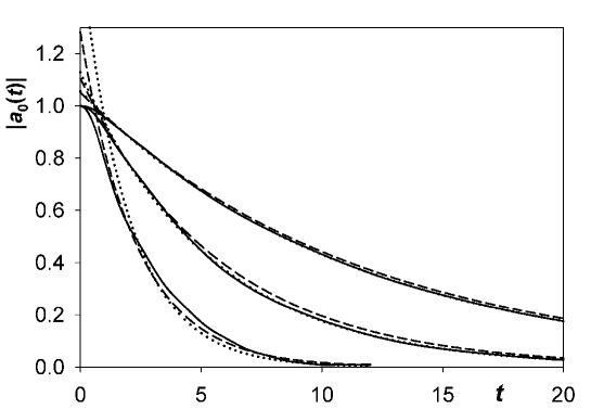
Figure 11: The dependence of the amplitude $a_{0}(t)$ decay vs. time. Parameter $E=1$. Parameter $C$ from up to down in the figure: $C^{2}=0.1;\,0.2;\,0.5$. Solid lines – numerical results; dashed lines – the pole approximations (43); dotted lines – the perturbation theory (48).

Appendix C

Consider now the case when $E>2-C^{2},\,\,(C^{2}<2)$ and when there exists one localized bounded state. We find the eigenstate $\overrightarrow{\Psi}_{\rm loc}$ localized at the lattice end and solve Schrödinger equation $H\overrightarrow{\Psi}_{\rm loc}=\varepsilon\overrightarrow{\Psi}_{\rm loc}$ (for the hamiltonian $H$ see (1)). The solution has the form of exponentially decaying function of $j$:

$$\overrightarrow{\Psi}_{\rm loc}=A\left\{\dfrac{1}{C},\,\alpha^{j-1}\right\},\quad A=\left(\dfrac{1}{C^{2}}+\dfrac{\alpha^{2}}{1-\alpha^{2}}\right)^{-1/2}.$$ (49)

Parameter $\alpha$ is expressed through the energy $\varepsilon$:

$$\alpha=\dfrac{1}{2}\,\left(\varepsilon-\sqrt{\varepsilon^{2}-4}\right).$$ (50)

Energy $\varepsilon$ is related to parameters $E$ and $C$ by the relationship, coinciding with given by (17):

$$E=\varepsilon\,\left(1-\dfrac{C^{2}}{2}\right)+\dfrac{C^{2}}{2}\sqrt{\varepsilon^{2}-4}\,.$$ (51)

Expand now the total wave function in terms of the eigenfunctions of the hamiltonian:

$$\overrightarrow{\Psi}=D\,\overrightarrow{\Psi}_{\rm loc}\,\exp(-i\varepsilon t)+{\rm C.C.S.},$$ (52)

where C.C.S. means the contribution from the continuous spectrum. The first term is just the contribution to amplitude from the localized state. It is necessary to find the constant $D$. To do this we consider the scalar product of the localized and the complete wave functions. Because of the orthogonality of wave functions one can get: $\left<\vec{\Psi}_{\rm loc}\vec{\Psi}\right>=D\exp(-i\varepsilon t)$. In this equality we put $t=0$. As the wave function is fully localized on the impurity site at $t=0$, i.e. $\vec{\Psi}(t=0)=(1,0,0,\ldots)$, then it follows that $D=\Psi_{\rm loc}^{*}(j=1)$. Thus, the necessary contribution to the amplitude on the impurity site from the localized state is:

$$a_{0}^{\rm loc}=\left|\Psi_{\rm loc}(1)\right|^{2}\exp(-i\varepsilon t).$$ (53)

Substituting the expression $\Psi_{\rm loc}(1)=AC^{-1}$ from (49) and expressing $A$ through $\varepsilon$ (see (50)) we get the final answer, coinciding with (17):

$$a_{0}^{\rm loc}(t)=\dfrac{\exp(-i\varepsilon t)}{1+\dfrac{C^{2}}{2}\left(\dfrac{\varepsilon}{\sqrt{\varepsilon^{2}-4}}-1\right)}.$$ (54)

References

- (1) K.E. Augustyn, J.C. Genereux, J.K. Barton. Angew. Chem. Int. Ed. 46, 5731 (2007).
- (2) J.K. Barton, E.D. Olmon, P.A. Sontz. Coord. Chem. Rev. 255, 619 (2011).
- (3) J.C. Genereux, J.K. Barton. Chem. Rev. 110, 1642 (2010).
- (4) S.S. Mallajosyula, S.K. Pati. J. Phys. Chem. Lett. 1, 1881 (2010).
- (5) B. Giese. Annu. Rev. Biochem. 71, 51 (2002).
- (6) J.D. Slinker, N.B. Muren, S.E. Renfrew, J.K. Barton. Nature Chem. 3, 228 (2011).
- (7) B. Giese. Bioorganic and Medicinal Chemistry 14, 6139 (2006).
- (8) J. Gao, P. Müller, M. Wang, S. Eckhardt, M. Lauz, K.M. Fromm, B. Giese. Angew. Chem. Int. Ed. 50, 1926 (2011).
- (9) A.V. Malyshev. Phys. Rev. Lett. 98, 096801 (2007).
- (10) J.C. Genereux, S.M. Wuerth, J.K. Barton. J. Am. Chem. Soc. 133, 3863 (2011).
- (11) H.T. Quan, Z. Song, X.F. Liu, P. Zanardi, C.P. Sun. Phys. Rev. Lett. 96, 140604 (2006).
- (12) Ph. Jacquod, I. Adagideli, C.W.J. Beenakker. Phys. Rev. Lett. 89, 154103 (2002).
- (13) F. M. Cucchietti, D.A.R. Dalvit, J.P. Paz, W.H. Zurek. Phys. Rev. Lett. 91, 210403 (2003).
- (14) T. Prosen, T.H. Seligman, M. Znidaric. arXiv:quant-ph/0304104.
- (15) G. Manfredi, P.-A. Hervieux Phys. Rev. Lett. 97, 190404 (2006).
- (16) V.A. Benderckii, L.A. Falkovsky, E.I. Kats. Pis’ma v ZhETF 86, 249 (2007).
- (17) V.A. Benderckii, E.I. Kats. Pis’ma v ZhETF 88, 386 2008.
- (18) V.A. Benderckii, E.I. Kats. Pis’ma v ZhETF 94, 494 (2011).
- (19) E. Fermi, J. Pasta, S. Ulam. Los Alamos report LA-1940 (1955).
- (20) . G.P. Berman, F.M. Izrailev. CHAOS 15, 015104 (2005).
- (21) A.A. Ovchinnikov, N.S. Erikhman, K.A. Pronin. Vibrational-Rotational Excitations in Nonlinear Molecular Systems. Kluwer Acedemic/Plenum Publishers, New York, 2001, P. 298.
- (22) R. Zwanzig. Lect. Theor. Phys.. 3, 106 (1960).
- (23) B. Elias, J.C. Genereux, J.K. Barton. Angew. Chem. Int. Ed. 47, 9067 (2008).
- (24) I.S. Gradstein, I.M. Ryzhik. Table of Integrals, Series, and Products. 7th Ed. Elsevier, Amsterdam 2007.