Error-Driven Dynamical $hp$-Meshes with the Discontinuous Galerkin Method for Three-Dimensional Wave Propagation Problems

Abstract

An $hp$-adaptive Discontinuous Galerkin Method for electromagnetic wave propagation phenomena in the time-domain is proposed. The method is highly efficient and allows for the first time the adaptive full-wave simulation of large, time-dependent problems in three-dimensional space. Refinement is performed anisotropically in the approximation order $p$ and the mesh step size $h$ regardless of the resulting level of hanging nodes. For guiding the adaptation process a variant of the concept of reference solutions with largely reduced computational costs is proposed. The computational mesh is adapted such that a given error tolerance is respected throughout the entire time-domain simulation.

1 Introduction

In this article, we are concerned with adaptively solving the Maxwell equations for electromagnetic fields with arbitrary time dependence in a three-dimensional domain such that a prescribed error tolerance is respected. In order to achieve this goal the Discontinuous Galerkin Method (DGM) [1, 2] is applied on anisotropic $hp$-meshes, which dynamically and autonomously adapt as the electromagnetic fields evolve. The mesh refinement is driven by a robust local error estimate based on a modification of the so-called method of reference solutions [3, 4] with largely reduced numerical costs.

The DG method has gained wide acceptance as a high order numerical method, which is very well-suited for time-domain problems. It combines the usually opposing key features of high order accuracy and flexibility. In particular, the method can easily deal with meshes containing hanging nodes, which makes it particularly well suited for $hp$-adaptivity. There is a well established body of literature on the DG method for various types of problems available. It has been thoroughly investigated by several research groups (see e.g. [5, 6, 7] and references therein). Concerning Maxwell’s equations in time-domain, the DGM has been studied in particular in [7, 8, 9, 10]. The latter two make use of hexahedral meshes, which allow for a computationally more efficient implementation [11].

The simplest approach to adapted grids consists of static a priori $h$-refinement around edges and corners, i.e., the possible locations of field singularities [12]. While this approach mitigates negative effects of fields singularities on the global solution accuracy, the level of refinement to be applied for achieving a certain accuracy is unknown. Moreover, edges and corners require no mesh refinement while there is no field, for instance, before illumination by a wave or after scattering took place. It also remains unclear how to choose polynomial orders in the remaining mesh. For these reasons our focus is on $hp$-adaptivity based on error estimations of the time-dependent solution.

Mesh refinement and specifically $hp$-adaptation has received considerable and continuous attention. The first published work on $h$-, $p$- and $hp$-adaptivity within the DG framework is presumably [13], where the authors considered linear scalar hyperbolic conservation laws in two-dimensional space. Hyperbolic problems have also been addressed, e.g., by Flaherty, Shephard and co-workers who considered two-dimensional problems in [14, 15] as well as three-dimensional settings with pure $h$-refinement in [16, 17]. A large number of contributions has been authored by Houston and various co-workers. They present a number of approaches to adaptivity and deal with first-order hyperbolic problems in [18, 19], using adjoint solutions [19, 20] or estimating errors in an energy norm [21, 22]. The contributions have a clear focus on the rigorous derivation of error estimates and error bounds. Applications are limited to one or two space dimensions. Recently, Solin and co-workers published papers, where they apply dynamical $hp$-meshes for various coupled problems including electromagnetics in two space dimensions [23, 24, 25]. They employ the concept of reference solutions for controlling mesh adaptivity and perform refinements, which are fully anisotropic in both mesh parameters $h$ and $p$. The application of reference solutions in their original form is numerically very expensive. In [25] it is stated that the solution of large three-dimensional problems would require distributed parallel computing.

In this paper, we propose a modification of the concept of reference solutions with drastically reduced numerical costs, which makes such simulations feasible. At the same time the key advantages are maintained, in particular its robustness and the independence of a particular set of underlying partial differential equations. The increased efficiency comes at the price of losing some sharpness in the error estimate. Like the original formulation, the proposed algorithm is entirely devoid of tuning parameters, and it reduces the true approximation error, i.e., it is not based on residuals or heuristic measures such as steep gradients. The adaptation can be performed in four major modes: isotropic in $h$ and $p$, anisotropic in one of $h$ or $p$, and fully anisotropic in $h$ and $p$. Unconstrained refinement in $h$ is possible because we allow for high level hanging nodes. The number of degrees of freedom (DoF) in a discretization will usually decrease from the former to the latter mode, while the computational load for finding the adapted mesh increases. However, we will show below that great savings in both, the number of DoF and computational time can be achieved by using fully anisotropic adaptivity.

The remainder of this article is organized as follows. In Sec. 2 the notation and Finite Element Spaces (FES) are introduced, which are applied for obtaining a weak DG formulation of Maxwell’s equations. Section 3 is devoted to the mesh refinement algorithm. First the individual steps, which constitute an adaptive algorithm are discussed. They are error estimation, element marking, the $h$–$p$-decision and the actual mesh adaptation. For each step a brief description with a review of the state of the art is provided, before we proceed with the details of our realization of each step in the Sections 3.1 to 3.5. Examples are presented in Sec. 4, which include a waveguide and an antenna radiation problem. Section 5 summarizes the findings and concludes the article.

2 Discretization of Maxwell’s Equations

In the following we assume resting, heterogeneous, linear, isotropic, non-dispersive and time-independent materials. Then, the magnetic permeability, $\mu$, and dielectric permittivity, $\epsilon$, are scalar values depending on the spatial position only. Under these assumptions Maxwell’s equations read

$$\nabla\times{\bf{E}}({\bf{x}},t) = -\mu({\bf{x}})\frac{\partial}{\partial t}{\bf{H}}({\bf{x}},t),$$ (1)

$$\nabla\times{\bf{H}}({\bf{x}},t) = {\color[rgb]{1,1,1}-}\epsilon({\bf{x}})\frac{\partial}{\partial t}{\bf{E}}({\bf{x}},t)+{\bf{J}}({\bf{x}},t),$$ (2)

with the spatial variable ${\bf{x}}\in\Omega\subset\mathbb{R}^{3}$ and the temporal variable $t\in[t_{0},T]\subset\mathbb{R}$ subject to boundary conditions specified at the domain boundary $\partial\Omega$ and initial conditions specified at time $t_{0}$. The electric and magnetic field vectors are denoted by ${\bf{E}}$ and ${\bf{H}}$, ${\bf{J}}$ denotes the electric current density.

Discretizations of Maxwell’s equations using the Discontinuous Galerkin Method have been obtained among others in [7, 8, 9, 10]. We will follow the framework and notation described in our previous work [26], which makes use of hexahedral meshes and modal basis functions as introduced in [10].

2.1 Notation

We denote by $\mathcal{T}_{h}$ a tessellation of the domain of interest $\Omega$ composed from non-overlapping hexahedra $\mathcal{T}_{i}$ such that $\mathcal{T}_{h}=\bigcup_{i=1}^{N}\mathcal{T}_{i}$ covers $\Omega$. The tessellation is required to be derivable from a regular root tessellation $\mathcal{T}_{0}$ by means of element bisections. However, we do not demand the resulting tessellation to be regular, i.e., we allow for hanging nodes and specifically for high level hanging nodes. The number of bisections performed for obtaining element $\mathcal{T}_{i}$ is denoted by $L_{i}$ in the isotropic and $L_{d,i}$ in the anisotropic case where $d$ corresponds to any of the spatial coordinates $\{x,y,z\}$. We call the intersection of two neighboring elements $\mathcal{T}_{i}\cap\mathcal{T}_{k}$ their interface $\mathcal{I}_{ik}$. In non-conformingly refined meshes, every face $\mathcal{F}_{j}$ of a hexahedral element may be partitioned into several interfaces depending on the number of neighbors $K$ such that $\mathcal{F}_{j}=\bigcup_{k=1}^{K}\mathcal{I}_{ik}$. This is an important difference to most other works including [7, 9, 27], which require one-to-one neighborhood relations. The (inter-)face orientation is described by the outward pointing unitary normal $\mathbf{n}_{j}$. The union of all faces is denoted by $\mathcal{F}$. The volume and edge length measures of element $i$ are denoted by $|\mathcal{T}_{i}|$ and $|\mathcal{T}_{d,i}|$.

2.2 Finite Element Spaces and Approximations

In DG methods trial and test functions are defined with element-wise compact support

$$\varphi_{i}^{p}({\bf x})=\begin{cases}\varphi^{p}({\bf x}),&\mathbf{x}\in\mathcal{T}_{i},\\ 0,&\text{otherwise}.\end{cases}$$ (3)

Cartesian grids allow the application of tensor product basis functions of the form

$$\varphi^{p}({\bf{x}})=\bigotimes_{d\,\in\,\{x,y,z\}}\varphi^{p_{d}}(d),$$ (4)

where $p$ is a multi-index obtained from all $p_{d}=0..P_{d}$. The local finite element spaces $\mathcal{V}^{P}({\mathcal{T}_{i}})$ spanned by the basis functions are given by the tensor product of the respective one-dimensional spaces

$$(\mathcal{V}^{P})_{\mathcal{T}_{i}}=(\mathcal{V}_{x}^{P_{x}})_{\mathcal{T}_{x,i}}\otimes(\mathcal{V}_{y}^{P_{y}})_{\mathcal{T}_{y,i}}\otimes(\mathcal{V}_{z}^{P_{z}})_{\mathcal{T}_{z,i}},\hskip 2.84526pt\text{where}$$ (5)

$$(\mathcal{V}_{d}^{P_{d}})_{\mathcal{T}_{d,i}}=\text{span}\{\varphi_{i}^{p_{d}}(d);\,0\leq p_{d}\leq P_{d}\}.$$ (6)

The approximation may, thus, make use of different orders $P_{d}$ in each of the coordinate directions, where the subscript is dropped if they are equal. We do not choose an interpolatory basis but follow a spectral approach and apply Legendre polynomials scaled such that [10]

$$\int_{\mathcal{T}_{d,i}}\varphi^{p_{d}}_{i}(x)\varphi^{q_{d}}_{i}(x)\,\text{d}x=\begin{cases}|\mathcal{T}_{d,i}|,\quad&p_{d}=q_{d}\\ 0,\quad&\text{otherwise}.\end{cases}$$ (7)

Associating an FES (5) with each element $\mathcal{T}_{i}$ of the tesselation defines the Finite Element discretization, where the electric and magnetic field approximations ${\bf E}_{h}$ and ${\bf H}_{h}$ are represented as

$${\bf E}({\bf x},t)\approx{\bf E}_{h}({\bf x},t)=\bigoplus_{i=1}^{N}{\bf E}_{i}({\bf x},t),\quad\quad{\bf H}({\bf x},t)\approx{\bf H}_{h}({\bf x},t)=\bigoplus_{i=1}^{N}{\bf H}_{i}({\bf x},t),$$ (8)

with the element local representations

$${\bf E}_{i}({\bf x},t)=\sum_{p}{\bf e}^{p}_{i}(t)\varphi^{p}_{i}({\bf x}),\quad\quad{\bf H}_{i}({\bf x},t)=\sum_{p}{\bf h}^{p}_{i}(t)\varphi^{p}_{i}({\bf x}).$$ (9)

The time-dependent vectors of coefficients ${\bf{e}}=({\bf{e}}_{1}^{0},..,{\bf{e}}_{1}^{P},..,{\bf{e}}_{N}^{0},..,{\bf{e}}_{N}^{P})^{\text{T}}$ and ${\bf{h}}=({\bf{h}}_{1}^{0},..,{\bf{h}}_{1}^{P},..,{\bf{h}}_{N}^{0},..,{\bf{h}}_{N}^{P})^{\text{T}}$ are the numerical degrees of freedom.

2.3 Weak DG formulation

Following the Galerkin procedure (1) and (2) are multiplied by a test function $\psi$ and integrated over the domain $\Omega$. Due to the compact support property (3) the integration can be carried out over every element $\mathcal{T}_{i}$ individually. Next, we perform integration by parts of the curl-terms and replace the exact field solution with the approximations (8). This leads to the semi-discrete variational problem of finding ${\bf{e}}$ and ${\bf{h}}$ such that

$$\int_{{\mathcal{T}_{i}}}\psi\,\mu\frac{\partial}{\partial t}{\bf H}_{h}\>\text{d}^{3}{\bf x}-\int_{{\mathcal{T}_{i}}}(\mathbf{\nabla}\psi)\times{\bf E}_{h}\>\text{d}^{3}{\bf x}+\int_{\partial{\mathcal{T}_{i}}}\psi\,(\mathbf{n}\times\widehat{\bf E}_{h})\,\text{d}^{2}{\bf x} = 0$$ (10)

$$\int_{{\mathcal{T}_{i}}}\psi\,\epsilon\frac{\partial}{\partial t}{\bf E}_{h}\>\text{d}^{3}{\bf x}+\int_{{\mathcal{T}_{i}}}(\mathbf{\nabla}\psi)\times{\bf H}_{h}\>\text{d}^{3}{\bf x}-\int_{\partial{\mathcal{T}_{i}}}\psi\,(\mathbf{n}\times\widehat{\bf H}_{h})\>\text{d}^{2}{\bf x} = 0,$$ (11)

$\forall i=1,..,N;\,\forall\psi\in\mathcal{V}_{i}$. For the above equations to be well-defined it is required that $\psi\in H^{1}$ in the interior of ${\mathcal{T}_{i}}$, which is fulfilled for the chosen Legendre basis. Note that $\widehat{\bf E}_{h}$ and $\widehat{\bf H}_{h}$ denote the numerical trace of the electric and magnetic field, which is single-valued for each vector field component at element boundaries. Introducing the numerical trace is a necessary step for resolving the ambiguity of the numerical approximations (8) at element interfaces. Due to the definition of the basis function support in (3), the components for the vector fields ${\bf{E}}_{h}$ and ${\bf{H}}_{h}$ are single valued at all points ${\bf{x}}\in\mathcal{T}\backslash\mathcal{F}$ but double-valued for all ${\bf{x}}\in\mathcal{F}$. The numerical trace is computed as

$$\widehat{{\bf{E}}}_{ik}=\{\{{\bf{E}}\}\}_{\mathcal{I}_{ik}}+\gamma\frac{{\bf{n}}_{ik}\times\llbracket{\bf{H}}\rrbracket_{\mathcal{I}_{ik}}}{2\{\{Y\}\}_{\mathcal{I}_{ik}}},\quad\quad\widehat{{\bf{H}}}_{ik}=\{\{{\bf{H}}\}\}_{\mathcal{I}_{ik}}-\gamma\frac{{\bf{n}}_{ik}\times\llbracket{\bf{E}}\rrbracket_{\mathcal{I}_{ik}}}{2\{\{Z\}\}_{\mathcal{I}_{ik}}}.$$ (12)

Typical choices are the centered and upwind value obtained by setting $\gamma$ to zero or one, respectively, where the upwind value is the solution of the Riemannian problem [28]. Above $\{\{\cdot\}\}$ and $\llbracket\cdot\rrbracket$ denote the average and jump operators

$$\{\{{\bf{a}}\}\}_{\mathcal{I}_{ik}}=({\bf{a}}_{k|\mathcal{I}_{ik}}+{\bf{a}}_{i|\mathcal{I}_{ik}})/2,\quad\quad\llbracket{\bf{a}}\rrbracket_{\mathcal{I}_{ik}}={\bf{a}}_{k|\mathcal{I}_{ik}}-{\bf{a}}_{i|\mathcal{I}_{ik}}.$$ (13)

The intrinsic impedance and admittance are given as

$$Z=\sqrt{\frac{\epsilon}{\mu}},\quad Y=\frac{1}{Z}.$$ (14)

The surface integrals in (10) and (11) represent interelement fluxes, the volume integrals are referred to as the mass and stiffness terms according to standard FE nomenclature. In the following the dependence of the spatial and temporal variable is not written down explicitly.

Note that no assumptions on the grid regularity have been made in the derivation. This is in a sharp contrast with Finite Element Methods based on edge elements, which require augmentation by edge constraints if hanging nodes are to be included [4]. In DG-type methods non-regular grids are no methodological issue, they only make the implementation more involved. The relative ease of handling non-regular meshes combined with the strictly element-local character of the numerical approximation make DG methods an ideal candidate for $hp$-adaptivity.

3 Automatic and dynamic $hp$-adaptation

Devising an $hp$-adaptive algorithm requires four major steps.

1. Derivation of global and local error estimates

2. Definition of a marking strategy for assigning a refinement/derefinement label to each element

3. Deriving criteria for making the $h$–$p$-decision

4. Definition of the actual mesh refinement/derefinement operators

For each of these steps several alternatives are possible. We will briefly list a few popular techniques and describe the main underlying idea before describing the approach followed in this contribution along with the reasoning behind this choice.

3.1 Error Estimation

Error estimators or indicators can, for instance, be obtained by expressing a residual through the numerical approximation. Residual based estimators in the context of Maxwell’s equations have been developed, e.g., in [21, 26, 29], or in [30, 31] with applications outside electrodynamics. Highly accurate estimators can be constructed based on adjoint solutions [32, 33], where the latter one is applied in a DG setting. However, the accuracy of adjoint based estimators comes at the price of having to repeatedly solve for the adjoint problem in addition. Comprehensive overviews of error estimation techniques are found in [34, 35, 36].

In this article we employ the concept of reference solutions [3, 4, 37] for obtaining error estimates. A reference solution is a numerically computed approximation, which is assumed to be significantly more accurate than the present approximation. This can be achieved by performing one uniform $h$-refinement step combined with increasing the approximation order by one in the element under consideration. Obtaining a reference mesh by pure $p$-enrichment has been proposed as well. Both techniques provide a reference mesh based on hierarchic FES enrichment. We apply the concept in its original form for finding an initial $hp$-mesh and propose a modified, computationally much cheaper variant, which is applied during the transient analysis. We found this estimator to be very robust and find reliable estimates independent of the local solution smoothness. This is an important advantage over the residual based estimate proposed in [26].

The aim then is to find the minimal $hp$-mesh such that

$$\|{\bf{\varepsilon}}\|_{\mathcal{T}_{h}}=\|{\bf{u}}-{\bf{u}}_{hp}\|_{\mathcal{T}_{h}}=\bigg{(}\sum_{{\mathcal{T}_{i}}\in\mathcal{T}}\|{\bf{u}}-{\bf{u}}_{hp}\|_{{\mathcal{T}_{i}}}^{2}\bigg{)}^{\frac{1}{2}}\leq\mathtt{TOL},$$ (15)

where $\|\cdot\|_{\mathcal{T}_{h}}$ denotes the global $L^{2}$-norm, and it is taken into account that the solution is a vector field. In the following ${\bf{u}}$ is used for denoting the electromagnetic solution $({\bf{E}},{\bf{H}})$. As only the approximation ${\bf{u}}_{hp}$ is known but not the exact solution ${\bf{u}}$ the target (15) cannot be achieved directly. However, it can be achieved asymptotically as

$$\|{\bf{\varepsilon}}_{hp}\|_{\mathcal{T}_{h}}=\bigg{(}\sum_{{\mathcal{T}_{i}}\in\mathcal{T}}\|{\bf{u}}_{\text{ref}}-\Pi_{hp}{\bf{u}}_{\text{ref}}\|_{\mathcal{T}_{i}}^{2}\bigg{)}^{\frac{1}{2}}=\bigg{(}\sum_{{\mathcal{T}_{i}}\in\mathcal{T}}\|\varepsilon_{hp}\|_{\mathcal{T}_{i}}^{2}\bigg{)}^{\frac{1}{2}},$$ (16)

where $\Pi_{hp}$ is a projection operator from the enriched reference FES $\mathcal{V}_{\text{ref}}$ to a space $\mathcal{V}_{\text{c}}$ associated with a refinement candidate. The space $\mathcal{V}_{\text{c}}$ is reduced with respect to the reference space but enriched with respect to $\mathcal{V}_{\mathcal{T}_{i}}$ such that

$$\mathcal{V}_{\mathcal{T}_{i}}\subset\mathcal{V}_{\text{c}}\subset\mathcal{V}_{\text{ref}}.$$ (17)

Refinement can be anisotropic in one or both of the mesh parameters. From (16) it follows that the element-wise error estimate is given as

$$\|\varepsilon_{hp}\|_{\mathcal{T}_{i}}=\|{\bf{u}}_{\text{ref}}-\Pi_{hp}{\bf{u}}_{\text{ref}}\|_{\mathcal{T}_{i}}.$$ (18)

Given a reference solution, the global and local error estimates (16) and (18) are fully computable.

3.1.1 Initial Mesh

Starting from the root tesselation $\mathcal{T}_{0}$ with some uniform polynomial order $P_{0}$ a reference mesh is constructed by performing one uniform refinement step in $h$ and $p$. We note that this has not to be done globally, but it can rather be done consecutively with each element of the current tesselation. The DG approximation $f_{\mathcal{T}_{i}}$ of a given function $f$ on the element ${\mathcal{T}_{i}}$, is obtained by applying the orthogonal projection operator $\Pi$

$$f_{\mathcal{T}_{i}}=(\Pi f)_{\mathcal{T}_{i}}=\sum_{p}(\Pi^{p}f)_{\mathcal{T}_{i}}\,\varphi_{i}^{p}=\sum_{p}\frac{\left(\varphi_{i}^{p},f\right)_{\mathcal{T}_{i}}}{\left(\varphi_{i}^{p},\varphi_{i}^{p}\right)_{\mathcal{T}_{i}}}\varphi_{i}^{p},$$ (19)

where $(u,v)_{\mathcal{T}_{i}}$ denotes the inner product $\int_{\mathcal{T}_{i}}uv\,\text{d}{\bf{x}}$ on the element $\mathcal{T}_{i}$. Equipping the FES (5) with an inner product defines a Hilbert space. Hence, the above projector yields the best approximation in the $L^{2}$-sense. After projecting the initial data to the refined elements the approximation error $\varepsilon_{i}$ of element ${\mathcal{T}_{i}}$ is estimated using (18). This procedure is repeated for all elements of the current tesselation. The global error $\varepsilon_{hp}$ is obtained from (16). The construction of the initial $hp$-mesh terminates when the stopping criterion $\varepsilon_{hp}\leq\mathtt{TOL}$ is met.

3.1.2 Dynamical Mesh

In the construction of an optimal initial $hp$-mesh the reference solution at each iteration can be generated because the initial data is known exactly. Obviously, this approach cannot be transferred immediately to the transient analysis. In [23] the authors approach the transient case by employing Rothe’s method. In contrast to the widely used Method of Lines, Rothe’s method discretizes the time variable first while preserving continuity of the spatial variable. This approach allows for applying the same techniques in the transient analysis that were used for obtaining the initial mesh at the cost of having to solve for a system of equations in every time step.

For performance reasons we prefer to employ explicit time-integration. The straightforward extension in this case is to compute on two meshes, the $hp$-mesh fulfilling the error tolerance and its reference mesh. However, this approach can easily become prohibitively expensive, both in computing time and memory consumption as the reference mesh usually has about 15 to 60 times more DoF depending on the approximation order. Taking into account that, moreover, the reference solution largely exceeds the required accuracy and is employed for driving the adaptivity only, this solution does not appear to be ideal. This motivated us to seek a different approach.

To this end, we switch roles of the reference mesh and the mesh used for estimating the local error and claim that the approximation on the current $hp$-mesh is sufficiently accurate for serving as the reference solution. Then, we estimate the element error by comparing to a reduced FES. This FES can be obtained by derefining the mesh in $h$ and $p$, or in a significantly more efficient manner by reducing the approximation order $P$. The element-wise error estimate is computed as

$$\|\varepsilon_{hp}\|_{\mathcal{T}_{i}}=\|{\bf{u}}_{\text{ref}}-\Pi_{p}{\bf{u}}_{\text{ref}}\|_{\mathcal{T}_{i}}.$$ (20)

Here, the solution on the current $hp$-mesh is the reference solution and $\Pi_{p}$ is the projection operator to the $p$-reduced FES. Computing the estimate (20) is very cheap. As the basis is hierarchic it comes down to considering the highest order terms of the current approximation only

$${\bf{u}}_{\text{ref},{\mathcal{T}_{i}}}-\Pi_{p}{\bf{u}}_{\text{ref},{\mathcal{T}_{i}}}=\sum_{p=0}^{P}{\bf{u}}^{p}_{i}\varphi^{p}_{i}-\sum_{p=0}^{P-1}{\bf{u}}^{p}_{i}\varphi^{p}_{i},$$ (21)

where ${\bf{u}}_{i}^{p}$ denotes the vector of coefficients of order $p$ local to element ${\mathcal{T}_{i}}$. Recalling that $p$ and $P$ are multi-indices as defined in (4), the local error estimate (21) is computed as

$$\|\varepsilon_{hp}\|_{\mathcal{T}_{i}}=\|\Big{(}\sum_{p_{y}=0}^{P_{y}}\sum_{p_{z}=0}^{P_{z}}{\bf{u}}_{i}^{p_{x}p_{y}p_{z}}\varphi_{i}^{p_{x}p_{y}p_{z}}\Big{)}_{|p_{x}=P_{x}}+\>\Big{(}\sum_{p_{x}=0}^{P_{x}-1}\sum_{p_{z}=0}^{P_{z}}{\bf{u}}_{i}^{p_{x}p_{y}p_{z}}\varphi_{i}^{p_{x}p_{y}p_{z}}\Big{)}_{|p_{y}=P_{y}}+\>\Big{(}\sum_{p_{x}=0}^{P_{x}-1}\sum_{p_{y}=0}^{P_{y}-1}{\bf{u}}_{i}^{p_{x}p_{y}p_{z}}\varphi_{i}^{p_{x}p_{y}p_{z}}\Big{)}_{|p_{z}=P_{z}}\|_{\mathcal{T}_{i}}.$$ (22)

Evaluating the $L^{2}$-norm and inserting the scaling property (7) yields the following form of the estimate

$$\|\varepsilon_{hp}\|_{\mathcal{T}_{i}}=\Big{[}\Big{(}\big{(}\sum_{p_{y}=0}^{P_{y}}\sum_{p_{z}=0}^{P_{z}}\|{\bf{u}}_{i}^{p_{x}p_{y}p_{z}}\|_{2}^{2}\big{)}_{|p_{x}=P_{x}}+\>\big{(}\sum_{p_{x}=0}^{P_{x}-1}\sum_{p_{z}=0}^{P_{z}}\|{\bf{u}}_{i}^{p_{x}p_{y}p_{z}}\|_{2}^{2}\big{)}_{|p_{y}=P_{y}}+\>\big{(}\sum_{p_{x}=0}^{P_{x}-1}\sum_{p_{y}=0}^{P_{y}-1}\|{\bf{u}}_{i}^{p_{x}p_{y}p_{z}}\|_{2}^{2}\big{)}_{|p_{z}=P_{z}}\Big{)}|{\mathcal{T}_{i}}|\Big{]}^{1/2}.$$ (23)

It is an important feature that the computation of this estimate is highly efficient as no runtime quadratures have to be performed.

We admit that the approach of projecting the solution to a reduced FES instead of an enriched one negatively affects the accuracy of the error estimation. However, it drastically reduces computational costs rendering the method applicable for a much larger class of real world problems. In Sec. 4 we demonstrate the robustness and reliability of this approach.

3.2 Marking Strategy

Following the error estimation, each element is assigned one of the labels refine, derefine or retain according to the marking strategy. The marking strategy, hence, has a strong impact on the number of DoF in the computational mesh. Popular strategies include error equidistribution, the fixed fraction strategy or variable fraction strategies such as bulk-chasing, commonly known as Dörfler-marking. The goal of the former strategy is to equilibrate the local errors by refining or derefining elements such that $\varepsilon_{i}\approx\mathtt{TOL}/\sqrt{N}$, where $\varepsilon_{i}$ is the local error estimate and $\mathtt{TOL}$ is a user-defined error tolerance [38]. For the fixed and variable fraction strategies, the elements are ordered by their estimated error at each refinement step. Then, for the former approach, a fixed fraction of elements from the top and bottom are marked for refinement and derefinement. The variable fraction or Dörfler-marking on the other hand continues to mark elements from the top and bottom of the list until their accumulated error accounts for a certain percentage of the total error. This can be expressed as finding a minimal subset ${\mathcal{T}}^{+}_{h}$ and a maximal subset ${\mathcal{T}}_{h}^{-}$ of $\mathcal{T}_{h}$ such that $\sum_{{\mathcal{T}_{i}}\in\mathcal{T}_{h}^{\{+,-\}}}\varepsilon^{2}_{i}\geq\theta^{2}_{\{+,-\}}\sum_{{\mathcal{T}_{i}}\in{\mathcal{T}}_{h}}\varepsilon^{2}_{i}$, where the sign indicates refinement and derefinement. As the values of $\theta_{\{+,-\}}$ indicate fractions of the total error, the Dörfler-marking can be considered as a fixed fraction marking with respect to the total error. Often a few percent of the elements make up for more than 90 % of the total error, while most of the elements contribute to the total error by less than 5 %. As the situation might change throughout a time-domain simulation, we consider the variable fraction marking the most suitable for our problems.

Also for the element marking distinct strategies are applied for constructing the initial $hp$-mesh and during the transient analysis. For generating the initial $hp$-mesh, we perform Dörfler-marking. The number of mesh adaptation iterations required for obtaining the initial mesh depends on the fraction of the total error. Less iterations are performed for large fractions. However, this usually leads to a slightly larger number of DoF.

During the transient analysis a slightly altered marking strategy is employed. This strategy is a variable fraction strategy with respect to the number of elements as well as to the total error. For every mesh adaptation a minimal subset $\mathcal{T}_{h}^{+}$ is assembled such that

$$\sum_{{\mathcal{T}_{i}}\in\mathcal{T}_{h}^{+}}\varepsilon_{i}^{2}\geq\min\Big{(}\sum_{{\mathcal{T}_{i}}\in\mathcal{T}_{h}}\theta^{2}_{+}\varepsilon_{i}^{2},\max\>(\varepsilon_{hp}^{2}-\mathtt{TOL}^{2},0)\Big{)}.$$ (24)

Hence, the size of the minimal subset of elements to be refined is not larger than determined by the given fraction $\theta$, but it can be smaller if the global error is close to the prescribed tolerance. If the estimated global error is smaller than $\mathtt{TOL}$, the set is empty, and no elements are refined in this adaptation step. If we were to apply the marking strategy in the same way we did for obtaining the initial mesh, the algorithm would continue refining elements even if the estimated error is less than the tolerance.

As stated above, we assume that the approximation on the current $hp$-mesh is sufficiently accurate for serving as the reference solution. This statement should ideally be true for every element. Therefore, marking elements for derefinement has to be done with care. We recall that mesh adaptation during the transient analysis is a dynamic process. Therefore, elements suitable for derefinement, which are not marked as such in an adaptation step are again considered for derefinement in the next step. In the examples in Sec. 4, we show that the mesh derefinement works well despite the careful approach.

3.3 The $hp$-Decision

Following the decision on which elements to adapt, the kind of adaptation has to be chosen, i.e., $h$- or $p$-adaptation. This decision is guided by the local solution smoothness. It is well known that for sufficiently smooth solutions consecutive $p$-enrichment leads to exponential convergence, whereas $h$-refinement yields algebraic convergence rates only [39, 40].

Figure 1 illustrates the dependence of the convergence rate on the regularity. The waveforms depicted in the insets, i.e., a Gaussian and a trapezoidal waveform in one-dimensional space, are projected to spaces $\mathcal{V}^{P}$ with $P$ varying from zero to five. The plots show the global error measured in the $L^{2}$-norm. While the convergence rate increases from one to six with every increase of $P$ for the Gaussian waveform, convergence is limited to first order in the latter case.

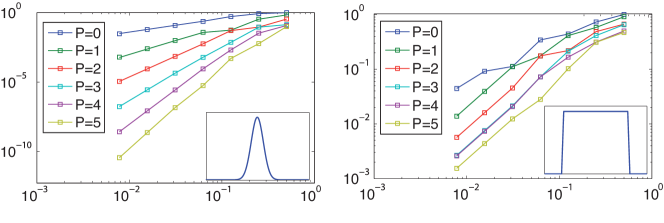
Figure 1: Global projection error of a Gaussian and a trapezoidal waveform as depicted in the insets. The plot in the left panel shows convergence of the error at a rate of $P+1$ for the Gaussian waveform. In the right panel, the low regularity limits convergence to first order.

However, exponential convergence in terms of DoF can be obtained even for locally non-smooth solutions as well by employing proper $hp$-refinement [39]. To this end, regions of low regularity are embedded into $h$-refined areas of the mesh using low order polynomials. Then, $p$-refinement is applied everywhere else. Thus, the performance of the adaptive method critically hinges on correct $hp$-decisions. In order to be in the position of performing anisotropic $hp$-refinement in three-dimensional space, we require information about the directional smoothness of the unknown solution.

A variety of techniques have been proposed for assessing the local smoothness or, more general, for making the $hp$-decision. The simplest ones makes use of information that is available a priori such as the position of field singularities due to edges and corners [12]. However, instead of relying on geometric information, we rather wish to drive the $hp$-decision based on the actual numerical solution. Known methods include the type parameter technique [41], ’Texas 3-Step’ [42], mesh optimization techniques [43], error prediction [44] or local regularity estimations [45, 46, 47, 48]. Descriptions of all methods are beyond the scope of this paper, and we refer to [49] for an extended overview including descriptions.

A particularly popular method is the estimation of the Sobolev regularity index $s$ in a local manner. One such technique is described briefly in the following, as it is illustrative for understanding why we pursue a different strategy. We focus on [46, 47], where the authors develop such a strategy based on monitoring the decay rate of the sequence of coefficients in the Legendre series expansion of the numerical solution. The drawback of this method and similar ones is that a certain number of coefficients is required for the computation of the coefficient decay rate to be robust. Taking into account that the Legendre coefficient of order zero provides information about the average in the element only, coefficients providing actual decay information start with the order of one. Hence, decay rate estimations require second order approximations as a minimum although higher order approximations will make the method more robust. Problems also occur if the solution exhibits a pronounced odd-even characteristic [50] leading to an alternation of small and large valued coefficients. The extension to problems in two- and three-dimensional space is possible but not unique, and the technique loses part of its clarity. As approximation orders of at least two have to be applied in all directions, this leads to a significant number of DoF also in elements, which do not require it.

As we wish to employ approximation orders as low as possible everywhere the solution permits, we follow a different approach. To this end, we reuse the reference solution at hand for finding the most suitable refinement from a list of candidates. This approach circumvents the issue of regularity estimation and the associated difficulties by testing various $h$-, $p$- and $hp$-candidates with respect to the reference solution. With this strategy, the best candidate naturally arises as the one offering the best ratio of approximation error $\varepsilon_{c}$ to the logarithm of its number of DoF ($\varepsilon_{c}/\log(\#\text{DoF})$).

The size of the list of candidates can vary considerably. It depends on the global refinement strategy, i.e. isotropic refinement only, fully anisotropic, or anisotropic in one of $h$ and $p$ only, but it also depends on the permissible increment and decrement in the $h$-refinement level $\Delta L$ and $\Delta P$. In this paper, we restrict both to one. However, candidates have to be competitive. This means that increasing the $h$-refinement level $L$, or $L_{d}$ in the anisotropic case, goes along with a reduction of $P$ in order to prevent a strong increase of the number of DoF in the element. The approximation order is reduced such that the number of DoF of the candidate is as small as possible but larger than the one of the current element ($\#\text{DoF}_{c}>\#\text{DoF}_{i}$). If isotropic refinement is applied two refinement candidates are obtained, one $h$-candidate, consisting of eight elements with possibly decreased approximation order $P$, and one $p$-candidate. For fully anisotropic refinement a number of fourteen candidates is considered, which are obtained by refining each of the mesh parameters $h$ or $p$ in one direction (three candidates), two directions (three candidates), and all three directions (one candidate). The approximation order $P$ of $h$-candidates is reduced as described above. The procedure above applies to mesh refinement. For the case of mesh derefinement, it is natural to proceed in a similar manner and set up derefinement candidates with a smaller number of DoF.

In the dynamic case, the procedure requires modification as the problem is encountered that a refined reference solution cannot be constructed. An error estimate is obtained by projecting to a $p$-reduced FES, however, given our description of regularity estimation based on coefficient decay rates, it is doubtful that regularity information can be extracted from a comparison of two solutions of the order $P$ and $P-1$ in a robust way. As there is not enough information available for making a reasoned $hp$-decision, the respective element is refined uniformly in $h$ and $p$. During the next mesh adaptation one or more of the refined elements might be derefined again according to the estimated error. Hence, it is during mesh derefinement only that anisotropic adaptation occurs.

3.4 Mesh Adaptation

At this point sufficient information is available for performing error driven $hp$-adaptation, which can be anisotropic in both mesh parameters $h$ and $p$. Upon mesh adaptation the numerical approximation given on the current $hp$-mesh ${\mathcal{T}_{h}}$ has to be transferred to the adapted mesh ${\mathcal{T}_{h}}^{*}$. The objective is to find the best representation of ${\bf{u}}_{hp}$ on ${\mathcal{T}_{h}}^{*}$ with respect to the $L^{2}$-norm. For all adaptations ($h$/$p$ refine/derefine) this is achieved by applying the orthogonal projection operator $\Pi$ introduced in (19). Due to the compact support of the basis, an unconstrained projection can be carried out in a strictly element-wise fashion. Additionally, the tensor product property of the basis (5) allows for performing the projection along each dimension individually. This reduces the three-dimensional quadrature of complexity order three in the number of quadrature nodes to a product of three one-dimensional quadratures of complexity order one. For the details of the projection we refer to [26], where the issues of optimality, stability and efficiency are investigated in details.

3.5 Comments on Practical Issues

During one time-domain simulation a very large number of adaptations is performed. These have to be administered in a way, which allows for an efficient traversing of all elements in each time step. Additionally, parent-child information is required for simplifying mesh derefinement. In this context, tree structures emerge as a suitable storage format. They allow for operating on the current discretization by working on the tree leaves only but contain the refinement history and parental relationships as well.

In the case of isotropic $h$-refinement, the tree is organized using octree-structures, where each of the eight children is assigned to one branch. In an octree-structure, every element and its associated node is either a non-reducible element of the root tesselation $\mathcal{T}_{0}$ or one of eight children of a single parent element. The depth of a node in the tree, i.e. the number of ancestor elements to the respective root element, corresponds to the number of consecutive $h$-refinements. This has been defined as the $h$-refinement level $L$ before.

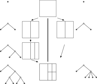
Figure 2: Comparison of mesh representation trees of different refinement histories. Starting from a single element (top) the final refinement at the bottom is obtained. For Option I in the left example only anisotropic refinement is applied, in Option II mixed anisotropic and isotropic refinement is employed. In this example, different representation trees are obtained for identical meshes. In the right hand example identical trees are obtained for identical final meshes although refinements were performed in a different order. Despite their identical appearance, trees III and IV differ, which becomes obvious when mesh derefinement is performed by cutting branches from the bottom up. These examples depict simple situations in two-dimensional space, in three dimensions more options arise.

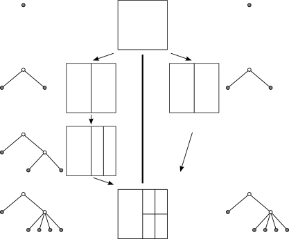
Figure 3: The same refinements as in Fig. 2 are performed. The representation tree is constructed following a minimal depth strategy. With this strategy the maximum depth of the representation tree corresponds to the maximum of the refinement levels $L_{d}$. Trees obtained with this strategy provide more freedom for performing mesh derefinement.

This organized view breaks down if non-anisotropic refinement is permitted. We refer to Fig. 2 for the following explanation. For the sake of clarity, a single two-dimensional element is considered. In Option I of the left hand side example only anisotropic $h$-refinement is applied. We extend the mesh representation tree in the same way as for isotropic refinement, i.e., the splitting of elements for every $h$-refinement is represented by extending the tree downwards from the respective node. In Option II, a combination of anisotropic and isotropic $h$-refinement is performed. This yields the same final mesh but a different representation tree. For the example on the right of Fig. 2, the same refinements are performed in a different order leading to identical final results and apparently identical representation trees.

The problem associated with the representation trees in Fig. 2 becomes visible when we attempt to derefine the mesh. This is achieved by cutting branches from the leaves upwards to the root, which immediately implies that derefinement has to occur exactly in the reversed refinement order. This is not a desired behavior, as the solution can develop in a way such that a different derefinement order would be more suitable. We point out, that the simple two-dimensional examples of Fig. 2 suggest that this is a minor issue. Nevertheless, in more complex situations in three-dimensional space it is a clear disadvantage if mesh refinement and derefinement have to be performed in reversed order.

The issue can be faced in a number of ways, many of them being computationally expensive. As one example, graph theory could be applied for generating a new minimal representation tree after each refinement. Our approach is computationally much cheaper and aims at constructing representation trees of minimal depth. The idea is illustrated in Fig. 3. In order to obtain a tree of minimal depth, a new generation of children is spawned only if the maximum $h$-refinement level $L=\max(L_{d})$ is increased. For the minimal tree I (Min. Tree I), this is the case for the first two refinements but not for the last refinement step. This strategy yields identical minimal representation trees I and II. However, the uniqueness of minimal trees is not guaranteed by the approach as demonstrated in the right hand example of Fig. 3. Nevertheless, for general refinements in three dimensions trees of a significantly smaller depth are obtained. They also provide a more intuitive representation as the tree depth connects with the maximum $h$-refinement level.

The important benefit of constructing minimal trees becomes evident when mesh derefinement is considered. In contrast to the trees constructed in Fig. 2, the derefinement order is not strictly prescribed by the refinement order. The minimal tree I allows for derefining such that the meshes at steps one or two are obtained. Additionally, a mesh with one horizontal and one vertical refinement of the right hand side element is obtained naturally. Using minimal trees, identical representations, such as I and II, always offer identical derefinement options, which is a significant advantage regarding the implementation in a computer code. Considering minimal tree III all meshes depicted in either of the options I or II can be obtained by derefinement.

The selection algorithm for the most suitable derefinement candidate is depicted in Fig. 4, where the mesh of the right hand example in Fig. 3 and minimal tree III is considered. Only the right hand half is depicted as derefinement of the other half is carried out analogously. Given the current discretization and its representation tree, we move one level upwards in order to obtain the topological parent element. The parent is the first $h$-derefinement candidate. Then, successively all possible $h$-refinements of the parent are performed such that $L_{d,c}\leq L_{d}$ is respected. The additional $h$-candidates for the considered example are depicted in the third row of Fig. 4. In a third step, the purely topological $h$-candidates are assigned FES of different orders $P$ yielding $hp$-candidates. We restrict the generation of $hp$-candidates in the sense that all elements of a candidate have the same order $P$. However, each $h$-candidate has its own $P$ dictated by the requirement that the number of DoF of the candidate has to be smaller than in the current mesh. In a last step, we compute $\varepsilon_{c}/\log(\#\text{DoF})$ for each $hp$-candidate and choose the best derefinement option.

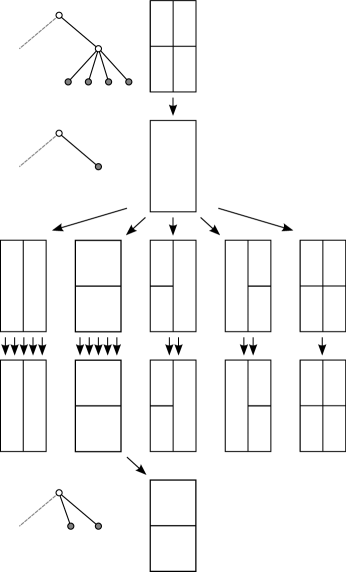
Figure 4: Illustration of the derefinement strategy using the right hand side example of Fig. 3 and minimal tree III as the starting point. Only the right hand half is depicted. In step one the topological parent is obtained. Next, the parent is $h$-refined again in order to generate a list of $h$-candidates. In step three $hp$-candidates are created by using different approximation orders for each $h$-candidate. This step is restricted in the sense that all elements of one candidate have same order $P$. Also, each candidate has to have less DoF than the current mesh. All candidates are tested yielding the winning $hp$-derefinement option.

4 Examples

4.1 Propagation in a waveguide

As a first example we consider the propagation of a wave packet in a rectangular waveguide. We consider a waveguide of type WR 19 working in U-Band. The cutoff frequency of the fundamental mode is 40 GHz. The frequency limit for single-mode operation is 60 GHz, and the wave packet considered has a frequency range of 45-59 GHz. The waveguide aperture dimensions are $4.78\times 2.39$ mm, and we consider a total length of 1 m corresponding to approximately 170 wavelengths. The purpose of this rather academic example is to demonstrate that the proposed algorithm can cope with situations where a very large number of adaptations has to be performed. Throughout the simulation the error tolerance has to be respected. Also, the number of DoF should remain approximately constant as the wave packet will largely keep its shape.

The generation of the initial $hp$-mesh required 28 iterations with the fraction $\theta$ as described in (24) set to 0.5. The series depicted in Fig. 5 shows the $hp$-mesh and the respective approximation of the $E_{y}$-component on the uniform root tesselation, at an intermediate iteration and the final $hp$-mesh. Refinement is allowed to be anisotropic in both mesh parameters, $h$ and $p$, though the algorithm applies no $h$-refinement in this case. This is reasonable as the solution is smooth. For depicting anisotropic $hp$-meshes we make use of a common visualization technique [3, 4]. To this end, each face is split into four triangles. The tensor product orders are coded with the triangle color. If the base edge of a green triangle is aligned with the $x$-axis, then $P_{x}=4$ according to the color legend. In the same way $P_{z}=5$ is represented with an orange triangle having its base edge aligned with the $z$-axis. This visualization allows for representing the orders in one plot and also gives an immediate impression of predominant directions regarding the approximation orders.

The highest orders in the initial mesh are $P_{x}=5$ and $P_{z}=6$. As the fundamental mode shows no variation in $y$-direction, no increase of $P_{y}$ occurs. The construction of the initial mesh requires seven seconds and yields close to 135,000 DoF. If we allow for isotropic refinement only, an initial mesh with 285,600 DoF is obtained within twelve seconds. Figure 6 shows the convergence graph of the approximation error with the number of DoF in a semi-logarithmic plot. In this graph, the error reduction occurs along an almost straight line showing exponential convergence.

Next, the time-domain simulation is performed. Figure 7 shows the $E_{y}$-component and the $hp$-mesh after the packet has traveled to the center and to the end of the waveguide. The performance of the adaptive algorithm is illustrated in Fig. 8. The top plot shows the evolution of the estimated global $L^{2}$-error normalized to the error obtained on the initial mesh. The middle and bottom plot depict the number of elements and DoF throughout the simulation. The data corresponds to 50 samples in time. The dispersion, which can be observed in Fig. 7 is a physical effect due to waveguide dispersion, not a numerical artifact. Code profiling showed that about 15 % of the computing time is spent for adaptation related tasks, which is almost negligible.

In order to assess the reduction in computing time and memory consumption due to adaptivity, simulations on fixed meshes were carried out. The number of DoF, memory consumption, runtime and error estimates after the final time step for various settings are listed in Tab. 1. In comparison to the adaptive solution factors of about three to six are observed regaring computing time and memory consumption on meshes using anisotropic approximation orders. For isotropic orders these factors increase to about 20.

#	Orders ($P_{x}/P_{y}/P_{z}$)	DoF / $10^{3}$	Memory / MB	norm. Runtime	$L^{2}$-error / $10^{-5}$
1	5/1/6	1131	35.5	4.3	0.13
2	4/1/5	808	30.4	2.7	1.36
4	5/5/5	2911	62.7	10.3	1.31
5	6/6/6	4620	88.7	20.6	0.13
6	$hp$	125-140	4.7-5.3	1	1.01

Table 1: Performance of simulations of example 4.1 using fixed and adaptive meshes. The orders 5/1/6 correspond to highest orders obtained in the initial mesh (cf. Fig. 5). If these orders are used globally the error is much smaller than that of the adaptive solution. Reducing the orders to 4/1/5, however, exceeds the error of the adaptive solution by about 30 %. Memory consumption of these fixed mesh solutions exceeds the adaptive solution by factors of 7 and 6, runtime by factors of 4 and 3. This has to be put in relation with the fraction of the mesh that is being refined, which corresponds to approximately 8 % of the waveguide length. For comparison, two simulations using uniform orders of five and six are included, which leads to a significant increase of the number of DoF and runtime.

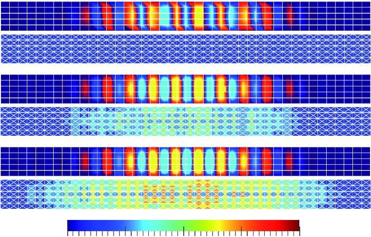
Figure 5: Generation of the initial $hp$-mesh for a Gauss-modulated sinusoidal waveform in the fundamental mode of a rectangular waveguide using anisotropic refinement. The $y$-component of the electric field and the $hp$-mesh is depicted in a cut view of a short waveguide section. The mesh is adapted iteratively such that the approximation error respects the tolerance $\mathtt{TOL}=10^{-5}$ in the global $L^{2}$-norm. Iteration #0 shows the approximation on the root tesselation and the initially uniform polynomial order. The adaptation terminates after 28 iterations, obtaining the initial $hp$-mesh depicted at the bottom. The autonomous adaptation algorithm employs $p$-enrichment only, which is desirable as the solution is smooth. The $hp$-meshes are depicted using a common tensor product visualization technique based on embedded triangles. The highest order $P_{z}$ employed in the initial $hp$-mesh is six. The respective $z$-oriented edges are part of orange colored triangles. The maximum of $P_{x}$ is five (yellow).

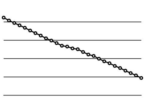
Figure 6: Convergence of the global $L^{2}$-error during construction of the initial $hp$-mesh as depicted in Fig. 5. The graph uses a logarithmic scale for the error and a linear one in the number of DoF, thus showing exponential convergence. The error tolerance of $10^{-5}$ in the global $L^{2}$-norm is met after 28 iterations.

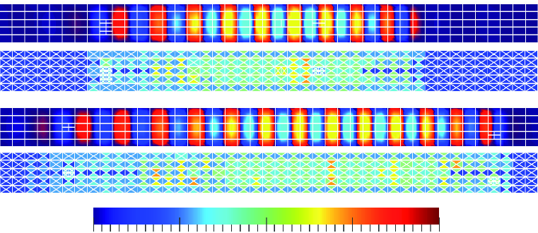
Figure 7: Evolution of the dynamic $hp$-mesh. Mesh refinement occurs predominantly in the form $p$-refinement. The snapshot show the field and mesh at the middle and end of the waveguide.

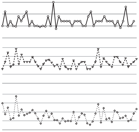
Figure 8: Temporal profiles of the global error normalized to the initial error (top, solid line with circles), number of elements (middle, dashed with triangles) and number of degrees of freedom (bottom, dotted line with diamonds). The time range covers the full time-domain simulation sampled at 50 instances.

4.2 Folded patch antenna

In this section a more complicated example is considered, where the farfield of a triple slot patch antenna fixed on a dielectric substrate is computed. The structure is taken from the examples of CST Microwave Studio as part of the CST Studio Suite [51]. It is illustrated in Fig. 9 with the defining points 1-13 of the patches given in Tab. 2. The relative permittivity of the substrate is 2.2. The substrate and metallization thicknesses are 0.813 mm and 0.2 mm, respectively. The antenna is excited using two discrete voltage ports, which impose a voltage across the gaps of the antenna feed at the position of points 2 and 3. The excitation voltage follows a Gaussian time profile with a standard deviation of 0.12 ns. The total simulation time is 2.5 ns.

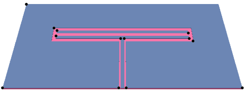
Figure 9: Triple slot folded patch antenna fixed on a dielectric substrate. The positions of the points in the $x$–$y$-plane are given in Tab. 2. The relative permittivity of the substrate is 2.2. The thicknesses of the substrate and the metallization are 0.813 mm and 0.2 mm, respectively.

Point	$x$ / mm	$y$ / mm	Point	$x$ / mm	$y$ / mm
1	-58.5	0	8	37	32
2	-1.7	0	9	-37	34
3	1.7	0	10	37	36
4	58.5	0	11	-37	38
5	39	30	12	-39	40
6	-1	32	13	-58.5	60
7	1	32

Table 2: Location of points 1-13 of Fig. 9 in the $x$–$y$-plane numbered from left to right and bottom up.

The farfield computation involves the determination of equivalent surface current densities on a collection surface $\Gamma$, and the subsequent solution of the Stratton-Chu integral under the farfield assumption

$${\bf{E}}_{\infty}({\bf{\hat{{\bf{x}}}}})=\frac{ik}{4\pi}\,\int_{\Gamma}[\hat{{\bf{x}}}\times{\bf{M}}({\bf{y}})+Z\hat{{\bf{x}}}\times(\hat{{\bf{x}}}\times{\bf{J}}({\bf{y}}))]e^{ik\hat{{\bf{x}}}\cdot{\bf{y}}}\,\text{d}A,$$ (25)

where $\hat{{\bf{x}}}$ is an observation direction, ${\bf{y}}$ the integration variable, $k$ the wave number and ${\bf{n}}$ the inward facing unit normal. The equivalent current densities on the collection surface are ${\bf{J}}({\bf{y}})={\bf{n}}\times{\bf{H}}({\bf{y}})$ and ${\bf{M}}({\bf{y}})={\bf{E}}({\bf{y}})\times{\bf{n}}$. As time-domain simulations are performed a Fourier transform of the equivalent currents involving the target frequency has to be carried out prior to solving (25).

In this example, the collection surface is a box enclosing the structure at a distance of 2 mm. Usually the mesh is constructed such that the collection surface is obtained as the union of faces of a number of connected elements. In this case the elements, which have to be considered for solving the farfield integral can be determined in a preprocessing step. As this advantage cannot be exploited on adaptive meshes, we allow for placing the collection surface $\Gamma$ independently of the mesh. The farfield integral is computed by dissecting $\Gamma$ into (mesh independent) patches and performing a Gauss-Legendre quadrature on each patch. The computational domain is terminated by Silver-Müller radiation boundary conditions.

The Figures 10 and 11 show snapshots of the electric field magnitude using a logarithmic color scale in the top left panel, the $hp$-mesh (top right), the elementwise error estimate (bottom left) and the element markers (bottom right). The viewplane is located at the bottom of the substrate. The physical times correspond to 0.3 ns and 0.9 ns. Tab. 3 summarizes the number of DoF, runtime and error estimates after the final time step for various adaptive and non-adaptive settings. The computing time and number of DoF is reduced by factors of about three to five.

The farfields computed from the reference and the setting of $\#2$ (cf. Tab. 3) are shown in Fig. 12. In this context, the approach presented in [52] is of interest, where the farfield error instead of the global solution error is employed for driving mesh adaptation.

#	$P$	$L$	Elements	DoF / $10^{3}$	norm. Time	$L^{2}$-error / $10^{-2}$	TOL / $10^{-2}$
1	3	—	11968	4596	1	0.89 (100 %)	—
2	1-3	0	11968	574-850	0.15	1.06 (119 %)	0.89
3	1-3	0-1	3542-7446	574- 1303	0.27	1.11 (125 %)	0.89
4	1-4	0-1	3542-6454	574- 1807	0.34	0.86 (97 % )	0.89
5	2	—	11968	1939	0.21	1.56 (175 %)	—
6	1	—	11968	574	0.03	4.60 (517 %)	—

Table 3: Performance of simulations of example 4.2 using fixed and adaptive meshes. The results given in the first row (#1) obtained on a static mesh of third order elements are taken as a reference. #2-#4 were obtained on various adaptive meshes. In particular, #2 was obtained using the same topological mesh as #1 using pure $p$-refinement with orders between one and three. Results #3 and #4 were obtained using a coarser root mesh with a maximum of one level of $h$-refinement. All adaptive simulations use as error tolerance the error of the reference, i.e. $0.89\cdot 10^{-2}$. This tolerance is not met in the cases #2 and #3, which is expected as the local resolution in every element is less or equal compared to the reference. In #4 a maximum order of 4 is permitted and the error tolerance is met. Results #5 and #6 employ the same topological mesh as the reference but uniform element orders of two and one, respectively. The computing time of #5 is comparable to the adaptive solutions, but it has a much larger error.

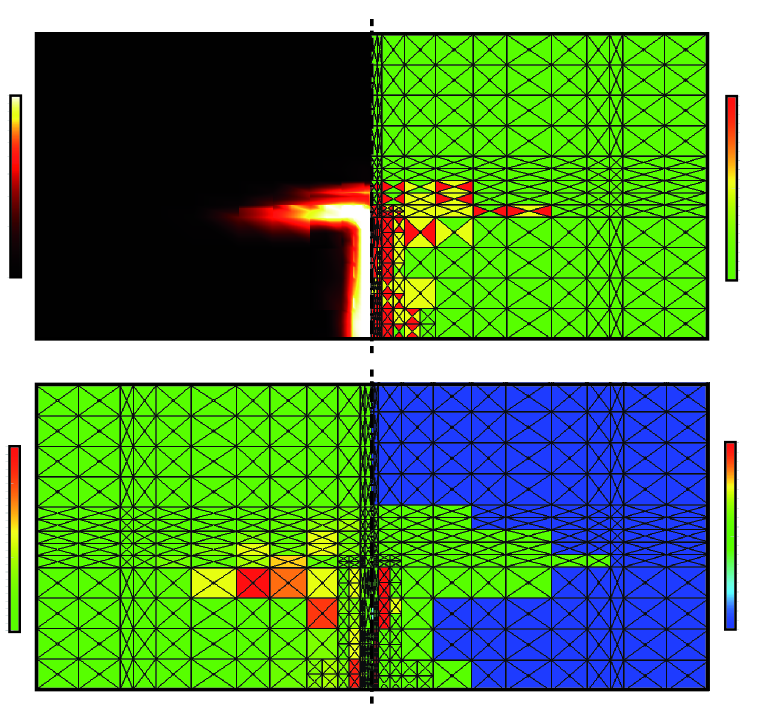
Figure 10: Snapshot at time 0.3 ns of the electric field magnitude with logarithmic color scale (top left), the $hp$-mesh (top right), the estimated error (bottom left) and the element marker (bottom right). The viewplane is located at the bottom of the substrate. A non-equidistant base mesh was used for capturing the edges of the patches. An element is marked as non-refinable/irreducible only if no more refinement/derefinement option ($h$ or $p$) is available, i.e., the given maximum/minimum $h$-level and order is met in all directions.

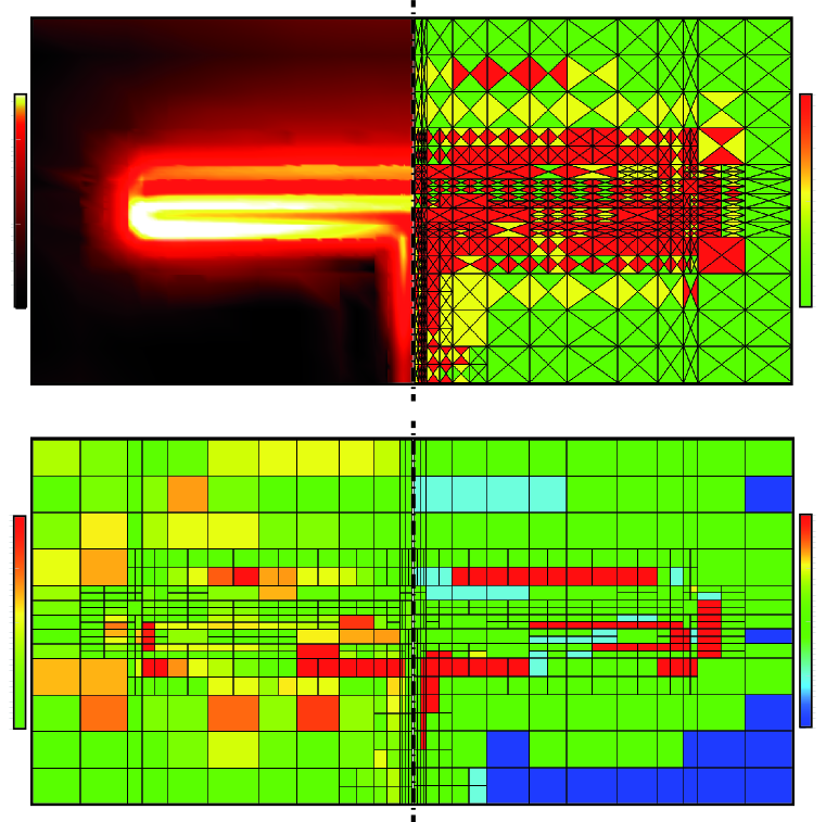
Figure 11: Snapshot at time 0.9 ns for the identical setup as in Fig. 10.

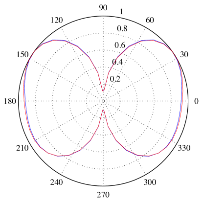
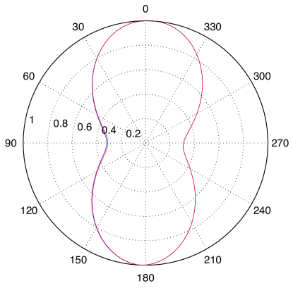
Figure 12: Normalized electric farfield at a frequency of 1.5 GHz of the triple slot patch antenna depicted in Fig. 9. The azimuth ($x$–$y$) and elevation ($z$–$x$) plane are shown in the left and right panels, respectively. Red curves correspond to the reference solution computed on a non-adaptive fine mesh using third order elements (cf. Tab. 3 #1), blue curves were obtained with the adaptive scheme and settings according to Tab. 3 #2.

5 Conclusion and Outlook

A scheme for performing time-domain simulations with the DG method on anisotropically refined dynamic $hp$-meshes in three-dimensional space was proposed. The adaptation is driven by the local solution error and guided by a novel variant of the concept of reference solutions. It drastically reduces the computational costs associated with error and regularity estimation allowing for the first time to perform fully automatic $hp$-adaptation for three-dimensional transient problems, where a given error tolerance is respected throughout the simulation. This was achieved by interchanging the role of the reference mesh and the solution mesh in the construction of the error estimate. While this comes at the cost of losing some sharpness of the estimate, it largely increases the practical applicability of the approach. The computation of the proposed error estimate is highly efficient as it is free of quadratures. Code profiling showed that for the presented examples the computational time consumed for all adaptivity related tasks was around 15 % of the total computing time.

The attainable savings in terms of computing time and memory consumption using dynamical $hp$-meshes strongly depend on the application. They roughly scale with the multi-scale character of the problem at hand and can reach factors above one hundred [26]. Here, two examples were shown, where computation times were reduced up to a factor of 20. Savings are particularly large with respect to implementations employing isotropic approximation orders only.

The implementation is currently restricted to orthogonal hexahedral meshes, which imposes limitations for the modeling of arbitrary structures. However, the proposed adaptation algorithm is independent of the actual element shape and can be applied on non-orthogonal curvilinear hexahedral meshes as well. This is the subject of ongoing work.

References

- Reed and Hill [1973] W. Reed, T. Hill, Triangular mesh methods for the neutron transport equation, Technical Report, Los Alamos Scientific Laboratory Report, 1973.
- LeSaint and Raviart [1974] P. LeSaint, P.-A. Raviart, On a finite element method for solving the neutron transport equation, Academic Press, 1974, pp. 89–123.
- Demkowicz [2007] L. Demkowicz, Computing with HP-Adaptive Finite Elements: Volume 1: One and Two Dimensional Elliptic and Maxwell Problems, Chapman & Hall/CRC, 2007.
- Solin et al. [2008] P. Solin, J. Cerveny, I. Dolezel, Arbitrary-level hanging nodes and automatic adaptivity in the hp-fem, Mathematics and Computers in Simulation 77 (2008) 117 – 132.
- Cockburn and Shu [2001] B. Cockburn, C. Shu, Runge–kutta discontinuous galerkin methods for convection-dominated problems, Journal of Scientific Computing 16 (2001) 173–261.
- Hesthaven and Warburton [2008] J. S. Hesthaven, T. Warburton, Nodal Discontinuous Galerkin Methods, Springer, 2008.
- Fezoui et al. [2005] L. Fezoui, S. Lanteri, S. Lohrengel, S. Piperno, Convergence and stability of a discontinuous galerkin time-domain method for the 3d heterogeneous maxwell equations on unstructured meshes, ESAIM-Math Model Num 39 (2005) 1149–1176.
- Hesthaven and Warburton [2002] J. S. Hesthaven, T. Warburton, Nodal high-order methods on unstructured grids i. time-domain solution of maxwell’s equations, Journal of computational physics 181 (2002) 186–221.
- Cohen et al. [2006] G. Cohen, X. Ferrieres, S. Pernet, A spatial high-order hexahedral discontinuous Galerkin method to solve Maxwell’s equations in time domain, Journal of Computational Physics 217 (2006) 340–363.
- Gjonaj et al. [2006] E. Gjonaj, T. Lau, S. Schnepp, F. Wolfheimer, T. Weiland, Accurate modelling of charged particle beams in linear accelerators, New Journal of Physics 8 (2006) 1–21.
- Wirasaet et al. [2010] D. Wirasaet, S. Tanaka, E. J. Kubatko, J. J. Westerink, C. Dawson, A performance comparison of nodal discontinuous galerkin methods on triangles and quadrilaterals, Int. J. Numer. Meth. Fluids 64 (2010) 1336–1362.
- Fahs et al. [2007] H. Fahs, S. Lanteri, F. Rapetti, A hp-like discontinuous Galerkin method for solving the 2D time-domain Maxwell’s equations on non-conforming locally refined triangular meshes, Technical Report, RR-6162, INRIA, http://hal.inria.fr/ inria-00140783/fr, 2007.
- Bey et al. [1995] K. S. Bey, A. Patra, J. T. Oden, hp-version discontinuous Galerkin methods for hyperbolic conservation laws: a parallel adaptive strategy, International Journal for Numerical Methods in Engineering 38 (1995) 3889–3908.
- Devine and Flaherty [1996] K. D. Devine, J. E. Flaherty, Parallel adaptive hp-refinement techniques for conservation laws, Applied Numerical Mathematics 20 (1996) 367–386.
- Remacle et al. [2003] J.-F. Remacle, J. Flaherty, M. Shephard, An adaptive discontinuous galerkin technique with an orthogonal basis applied to compressible flow problems, SIAM Review 45 (2003) 53–72.
- Flaherty et al. [1997] J. E. Flaherty, R. M. Loy, M. S. Shephard, B. K. Szymanski, J. D. Teresco, L. H. Ziantz, Adaptive Local Refinement with Octree Load Balancing for the Parallel Solution of Three-Dimensional Conservation Laws, Journal of Parallel and Distributed Computing 47 (1997) 139–152.
- Remacle et al. [2005] J.-F. Remacle, X. Li, M. S. Shephard, J. E. Flaherty, Anisotropic adaptive simulation of transient flows using discontinuous Galerkin methods, International Journal For Numerical Methods In Fluids 62 (2005) 899–923.
- Houston and Süli [2001] P. Houston, E. Süli, hp-adaptive discontinuous galerkin finite element methods for first-order hyperbolic problems, SIAM J. Sci. Comput. 23 (2001) 1226–1252.
- Houston et al. [2002] P. Houston, B. Senior, E. Süli, hp‐discontinuous galerkin finite element methods for hyperbolic problems: error analysis and adaptivity, International journal for numerical methods in fluids 40 (2002) 153–169.
- Hartmann and Houston [2003] R. Hartmann, P. Houston, Adaptive Discontinuous Galerkin Finite Element Methods for Nonlinear Hyperbolic Conservation Laws, SIAM J. on Numerical Analysis 24 (2003) 979–1004.
- Houston et al. [2005] P. Houston, I. Perugia, D. Schötzau, Energy norm a posteriori error estimation for mixed discontinuous galerkin approximations of the maxwell operator, Computer Methods in Applied Mechanics and Engineering 194 (2005) 499–510.
- Houston et al. [2007] P. Houston, D. Schötzau, T. P. Wihler, Energy Norm a Posteriori Error Estimation of hp-Adaptive Discontinuous Galerkin Methods for Elliptic Problems, Mathematical Models & Methods In Applied Sciences 17 (2007) 33–62.
- Solin et al. [2010] P. Solin, L. Dubcova, J. Kruis, Adaptive hp-FEM with dynamical meshes for transient heat and moisture transfer problems, Journal of Computational and Applied Mathematics 233 (2010) 3103–3112.
- Dubcova et al. [2010] L. Dubcova, P. Solin, J. Cerveny, P. Kus, Space and Time Adaptive Two-Mesh hp-Finite Element Method for Transient Microwave Heating Problems, Electromagnetics 30 (2010) 23–40.
- Korous and Solin [2012] L. Korous, P. Solin, An adaptive hp-DG method with dynamically-changing meshes for non-stationary compressible Euler equations, Computational Fluid Dynamics 2006 (2012) 1–20.
- Schnepp and Weiland [2012] S. M. Schnepp, T. Weiland, Efficient large scale electromagnetic simulations using dynamically adapted meshes with the discontinuous galerkin method, Journal of Computational and Applied Mathematics 236 (2012) 4909 – 4924.
- Hesthaven and Warburton [2004] J. Hesthaven, T. Warburton, High-order nodal discontinuous Galerkin methods for the Maxwell eigenvalue problem, Philosophical Transactions Of The Royal Society Of London Series A-Mathematical Physical And Engineering Sciences 362 (2004) 493–524.
- LeVeque [1990] R. J. LeVeque, Numerical Methods for Conservation Laws, Birkhäuser, 1990.
- Beck et al. [2002] R. Beck, R. Hiptmair, R. H. W. Hoppe, B. Wohlmuth, Residual based a posteriori error estimators for eddy current computation, ESAIM: Mathematical Modelling and Numerical Analysis 34 (2002) 159–182.
- Cockburn [2003] B. Cockburn, Discontinuous galerkin methods, Z. Angewandte Mathematische Mechanik (ZAMM) 83 (2003) 731–754.
- Barth [2005] J. Barth, Adaptive Mesh Refinement – Theory and Applications, Springer, 2005, pp. 183–202.
- Giles and Süli [2003] M. B. Giles, E. Süli, Adjoint methods for PDEs: a posteriori error analysis and postprocessing by duality, Acta Numerica 11 (2003) 145–236.
- Wang and Mavriplis [2009] L. Wang, D. J. Mavriplis, Adjoint-based h–p adaptive discontinuous Galerkin methods for the 2D compressible Euler equations, Journal of Computational Physics 228 (2009) 7643–7661.
- Verfürth [1996] R. Verfürth, A Review of a Posteriori Error Estimation and Adaptive Mesh-Refinement Techniques, Wiley-Teubner, 1996.
- Ainsworth and Oden [2000] M. Ainsworth, J. T. Oden, A posteriori error estimation in finite element analysis, Wiley-Interscience, 2000.
- Barth and Deconinck [2003] T. Barth, H. Deconinck (Eds.), Error Estimation and Adaptive Discretization Methods in Computational Fluid Dynamics, Lecture Notes in Computational Science and Engineering, Springer-Verlag, Berlin/Heidelberg, 2003.
- Solin et al. [2010] P. Solin, L. Dubcova, J. Cerveny, I. Dolezel, Adaptive hp-fem with arbitrary-level hanging nodes for maxwell’s equations, Advances in Applied Mathematics and Mechanics 2 (2010) 518–532.
- Chen [1994] K. Chen, Error equidistribution and mesh adaptation, SIAM Journal on Scientific Computing 15 (1994) 798–818.
- Babuska [1994] I. Babuska, The p and hp versions of the finite element method, basic principles and properties, SIAM review (1994).
- Schwab [1999] C. Schwab, p- and hp- Finite Element Methods: Theory and Applications to Solid and Fluid Mechanics, Oxford University Press, USA, 1999.
- Gui and Babuska [1986] W. Gui, I. Babuska, The h,p and h-p versions of the finite element method in 1 dimension. III. The adaptive h-p version, Numerische Mathematik 49 (1986) 659–683.
- Oden et al. [1992] J. T. Oden, A. Patra, Y. Feng, An hp adaptive strategy, Am Soc Mech Eng Appl Mech Div Amd 157 (1992).
- Rachowicz et al. [1989] W. Rachowicz, J. T. Oden, L. Demkowicz, Toward a universal h-p adaptive finite element strategy part 3. design of h-p meshes, Computer Methods In Applied Mechanics And Engineering 77 (1989) 181–212.
- Melenk and Wohlmuth [2001] J. M. Melenk, B. I. Wohlmuth, On residual-based a posteriori error estimation in hp-FEM, Advances in Computational Mathematics 15 (2001) 311–331 (2002).
- Ainsworth and Senior [1998] M. Ainsworth, B. Senior, An adaptive refinement strategy for hp-finite element computations, Applied Numerical Mathematics 26 (1998) 165–178.
- Houston et al. [2003] P. Houston, B. Senior, E. Süli, Sobolev regularity estimation for hp-adaptive finite element methods, F. Brezzi, A. Buffa, S. Corsaro, A. Murli, Editors, Numerical Mathematics and Advanced Applications (2003) 619–644.
- Houston and Süli [2005] P. Houston, E. Süli, A note on the design of hp-adaptive finite element methods for elliptic partial differential equations, Computer Methods in Applied Mechanics and Engineering 194 (2005) 229–243.
- Wihler [2011] T. P. Wihler, An hp-adaptive strategy based on continuous Sobolev embeddings, Journal of Computational and Applied Mathematics 235 (2011) 2731–2739.
- Mitchell and McClain [2011] W. Mitchell, M. A. McClain, A comparison of hp-adaptive strategies for elliptic partial differential equations, submitted for publication (2011).
- Klöckner et al. [2011] A. Klöckner, T. Warburton, J. S. Hesthaven, Viscous shock capturing in a time-explicit discontinuous Galerkin method, Mathematical Modelling of Natural Phenomena 6 (2011) 57–83.
- CST [????] CST – Computer Simulation Technology AG, Bad Nauheimer Str. 19, 64289 Darmstadt, Germany
- Monk and Süli [1999] P. Monk, E. Süli, The adaptive computation of far-field patterns by a posteriori error estimation of linear functionals, SIAM J. on Numerical Analysis 36 (1999) 251–274.