\publishers
affiliation: Institute of Integrative Biology, ETH Zurich
keywords: epidemiology, plant disease, mathematical model, host-pathogen interaction, fungicide resistance, population dynamics
corresponding author:
Alexey Mikaberidze (alexey.mikaberidze@env.ethz.ch)
Abstract
Mikaberidze, A., McDonald, B. A., Bonhoeffer, S. 2013. Can high risk fungicides be used in mixtures without selecting for fungicide resistance? Phytopathology.
Fungicide mixtures produced by the agrochemical industry often contain low-risk fungicides, to which fungal pathogens are fully sensitive, together with high-risk fungicides known to be prone to fungicide resistance. Can these mixtures provide adequate disease control while minimizing the risk for the development of resistance? We present a population dynamics model to address this question. We found that the fitness cost of resistance is a crucial parameter to determine the outcome of competition between the sensitive and resistant pathogen strains and to assess the usefulness of a mixture. If fitness costs are absent, then the use of the high-risk fungicide in a mixture selects for resistance and the fungicide eventually becomes nonfunctional. If there is a cost of resistance, then an optimal ratio of fungicides in the mixture can be found, at which selection for resistance is expected to vanish and the level of disease control can be optimized.
Fungicide resistance is a prime example of adaptation of a population to an environmental change, also known as evolutionary rescue [6, 24]. While global climate change is expected to result in a loss of biodiversity in natural ecosystems, evolutionary rescue is seen as a mechanism that may mitigate this loss. In the context of crop protection the point of view is quite the opposite: reducing adaptation of crop pathogens to chemical disease control would help stabilize food production. Better understanding of the adaptive process may help slow or prevent it. This requires a detailed quantitative understanding of the dynamics of infection and the factors driving the emergence and development of fungicide resistance [11]. Despite the global importance and urgency of fungicide resistance, this problem has received relatively little theoretical consideration (see [22, 21, 51, 42, 50, 37] and [11] for a comprehensive review) as compared, for example, to antibiotic resistance [40, 10, 34, 4].
In recent years, agrochemical companies have begun marketing mixtures that contain fungicides with a low-risk of developing resistance with fungicides that have a high-risk developing of resistance. In extreme cases the high-risk fungicide is no longer effective against some common pathogens because resistance has become widespread. For example, a large proportion of the European population of the important wheat pathogen Mycosphaerella graminicola (recently renamed Zymoseptoria tritici) [39, 41] is resistant to strobilurin fungicides [54].
A number of previous modeling studies addressed the effect of fungicide mixtures on selection for fungicide resistance (for example, [28, 52, 27, 49, 22, 23]). Different studies used different definitions of “independent action” (also called “additivity” or “zero interaction” in the literature) of fungicides in the mixtures [48] and reported somewhat different conclusions. One study [48] critically reviewed the outcomes of these earlier studies and attempted to clarify the consequences of using different definitions of “independent action”. Some studies found that alternations are preferable to mixtures [28], while others found that mixtures are preferable to alternations [52]. A more recent study [23] addressed this question using a detailed population dynamics model and found that in all scenarios considered, mixtures to provided the longest effective life of fungicides as compared to alternations or concurrent use (when each field receives a single fungicide, but the fungicides applied differ between the fields). This study used the Bliss’ definition of “independent action” of the two fungicides [9] (also called Abbot’s formula in the fungicide literature [1]).
We addressed the question of whether mixtures of low-risk and high risk fungicides can provide adequate disease control while minimizing further selection for resistance using a simple population dynamics model of host-pathogen interaction based on a system of ordinary differential equations. We found that the fitness cost associated with resistance mutations is a crucial parameter, which governs the outcome of the competition between the sensitive and resistant pathogen strains.
A single point mutation associated with fungicide resistance sometimes makes the pathogen completely insensitive to a fungicide, as is the case for the G143A mutation giving resistance to strobilurin fungicides in many fungal pathogens [15, 17]. In many other cases the resistance is partial, for example, resistance of Z. tritici and other fungi to azole fungicides [13, 57]. Therefore, we considered varying degrees of resistance in our model.
In contrast to our study, resistance in [22] was assumed to bear no fitness costs for the pathogen. It was found that in the absence of fitness costs the use of fungicide mixtures delays the development of resistance [22]. This conclusion is in agreement with our results (see Appendix A.4). Here we focus on finding conditions under which the selection for the resistant pathogen strain is prevented by using fungicide mixtures.
1 Theory and approaches
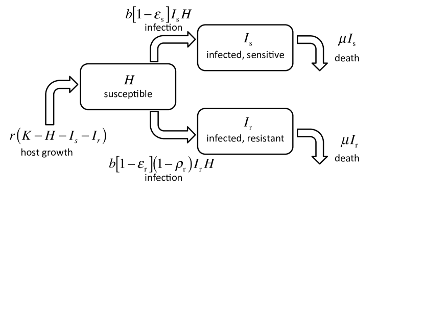
We use a deterministic mathematical model of susceptible-infected dynamics (see Fig. 1)
| (1) | ||||
| (2) | ||||
| (3) |
The model has three compartments: healthy hosts , hosts infected by a sensitive pathogen strain , hosts infected by a resistant pathogen strain ; and is similar to the models described in [11, 21]. The subscript “s” stands for the sensitive strain and the subscript “r” stands for the resistant strain. The quantities , and , represent the total amount of the corresponding host tissue within one field, which could be leaves, stems or grain tissue, depending on the specific host-pathogen interaction. Healthy hosts grow with the rate . Their growth is limited by the “carrying capacity” , which may imply limited space or nutrients. Furthermore, healthy hosts may be infected by the sensitive pathogen strain and transformed into infected hosts in the compartment with the transmission rate . This is a compound parameter given by the product of the sporulation rate of the infected tissue and the probability that a spore causes new infection. Healthy hosts may also be infected by the resistant pathogen strain and transformed into infected hosts in the compartment . In this case, resistant mutants suffer a fitness cost which affects their transmission rate such that it becomes equal to . The corresponding terms in Eqs. (1)-(3) are proportional to the amount of the available healthy tissue and to the amount of the infected tissue or . Infected host tissue loses its infectivity at a rate , where is the characteristic infectious period.
Since our description is deterministic we do not take into account the emergence of new resistance mutations but assume that the resistant pathogen strain is already present in the population. Therefore, when “selection for resistance” is discussed below, we refer to the process of winning the competition by this existing resistant strain due to its higher fitness with respect to the sensitive strain in the presence of fungicide treatment. Emergence of new resistance mutations is a different problem, which goes beyond the scope of our study and requires stochastic simulation methods. We do not consider the possibility of double resistance in the model, but by preventing selection for single resistance as described here, one would also diminish the probability of the emergence of double resistance for both sexually and asexually reproducing pathogens (see Appendix A.7).
We consider two fungicides A and B. Fungicide A is the high-risk fungicide, to which the resistant pathogen strain exhibits a variable degree of resistance. However, the sensitive strain is fully sensitive to fungicide A. Fungicide B is the low-risk fungicide, i. e. both pathogen strains are fully sensitive to it. We compare the effects of the fungicide A applied alone, fungicide B applied alone and the effect of their mixture in different proportions.
We assume that the fungicides will decrease the pathogen transmission rate [see the expression in square brackets in Eq. (2), Eq. (3)]. For example, application of a fungicide could result in production of spores that are deficient essential metabolic products such as ergosterol or -tubulin. Consequently, these spores would likely have a lower success rate in causing new infections. Spores of sensitive strains of Z. tritici produced shorter germ tubes when exposed to azoles [33]. Spores that produce shorter germ tubes are less likely to find and penetrate stomata, hence are less likely to give rise to new infections. Protectant activity of fungicides will also reduce the transmission rate [56, 46]. These studies [56, 46] also reported that fungicide application leads to a reduction in the number of spores produced. This outcome can be attributed to the fungicide decreasing the sporulation rate and thus affecting or decreasing the infectious period and thus affecting , or both of these effects. More detailed measurements are often needed to distinguish between these different effects.
When only one fungicide applied, the reduction of the transmission rate is described by
| (4) |
for the fungicide A, and by
| (5) |
for the fungicide B. These functions grow with the fungicide doses , and saturate to values , , respectively, which are the maximum reductions in the transmission rate (or efficacies). This functional form was used before in the fungicide resistance literature [21, 19]. We also performed the analysis for the exponential fungicide action more common in plant pathology and obtained qualitatively similar results. The reason for choosing the function in Eq. (5) was that it made possible to obtain all the results analytically. The parameters , represent the fungicide dose at which half of the maximum effect is achieved. These parameters can always be made equal by rescaling the concentration axis for one of the fungicides. Hence, we set .
We next determine the effect of a mixture of two fungicides according to the Loewe’s definition of additivity (or non-interaction) [7] (an equivalent graphic procedure is known as the Wadley method in the fungicide literature [35]). It is based on the notion that a compound cannot interact pharmacologically with itself. A sham mixture of a compound A with itself can be created and its effect used as a reference point for assessing of whether the components of a real mixture interact pharmacologically. When the two compounds A and B have the same effect as the sham mixture of the compound A with itself, they are said to have no interaction (or an additive interaction). In this case, the isobologram equation
| (6) |
holds (see Sec. VA of [7] for the derivation). Here, and are the doses of the compounds A and B, respectively, when applied in the mixture; is the isoeffective dose of the compound A, that is the dose at which compound A alone has the same effect as the mixture; and is the isoeffective dose of the compound B. If the mixture of A and B has a larger effect than the zero-interactive sham mixture, then and the two compounds are said to interact synergistically. On the contrary, when the mixture of A and B has a smaller effect than the zero-interactive sham mixture, and the two compounds interact antagonistically.
Using the dose-response dependencies of each fungicide when applied alone, Eq. (5) and Eq. (6), we derive the dose-response function for the combined effect of the two fungicides on the sensitive pathogen strain in the case of no pharmacological interaction (see Sec. VIB of [7] for the derivation):
| (7) |
Similarly, we determine the combined effect of the two fungicides on the resistant pathogen strain still without pharmacological interaction:
| (8) |
where we introduced , the degree of sensitivity of the resistant strain to the fungicide A (the high-risk fungicide). At the pathogen is fully resistant to fungicide A and the effect of the mixture in Eq. (8) does not depend on its dose , while at the pathogen is fully sensitive to fungicide A.
The expression in Eq. (7) and Eq. (8) are only valid in the range of fungicide concentrations, over which isoeffective concentrations can be determined for both fungicides. Here, the isoeffective concentration is the concentration of a fungicide applied alone that has the same effect as the mixture. This requirement means that we are only able to consider the effect of the mixture at a sufficiently low total concentration: .
Next, we introduce deviations from the additive pharmacological interaction. There are several ways to do this, usually by adding an interaction term to the isobologram equation [18]. We chose a specific form of the interaction term, which is proportional to the square root of the product of the concentrations of the two compounds [Eq. (28) in [18]]. Assuming , this form allows for a simple analytical expression for the effect of the combination on the sensitive strain
| (9) |
and on the resistant strain
| (10) |
Here , where is the dose of the fungicide A and is the dose of the fungicide B, is the proportion of the fungicide B in the mixture and
| (11) |
| (12) |
are the parameters which modify due to pharmacological interaction and partial resistance. Eqs. (9), (10) are obtained from Eq. (6) with an interaction term added and the dose-response functions of each fungicide when applied alone, Eq. (5). The degree of pharmacological interaction is characterized by the parameter . At the fungicides do not interact and Eqs (9), (10) are the same as Eqs (7), (8). The case when represents synergy: the interaction term proportional to in Eq. (9) and Eq. (10) is positive and it reduces the value of , meaning that the same effect can be achieved at a lower dose than at . The case when corresponds to antagonism (see Appendix A.1). Note, that the interaction term is proportional to . This functional form guarantees that it vanishes, whenever only one of the compounds is used, i. e. or .
In order to make clear the questions we ask and the assumptions we make, we consider the dynamics of the frequency of the resistant strain . The rate of its change is obtained from Eqs. (1)-(3)
| (13) |
where
| (14) |
is the selection coefficient [a similar expression was found in [19]]. Here and are given by Eq. (9) and Eq. (10). If , then the resistant strain is favored by selection and will eventually dominate the pathogen population ( at ). Alternatively, if , then the sensitive strain is selected and will dominate the population ( at ).
The focus of this paper is to investigate the parameter range over which , i. e. the sensitive strain is favored by selection. Mathematically this corresponds to finding the range of stability of the equilibrium (fixed) point of the system Eqs. (1)-(3), corresponding to , , . Our focus is mainly on the direction of selection. To address this point we do not need to assume that the host-pathogen equilibrium is reached. However, we explicitly assume that the host-pathogen equilibrium is reached during one season in Sec. 2.3, where we evaluate the benefit of fungicide treatment. The implications of this assumption are discussed at the beginning of Sec. 2.3. Furthermore, we assume that the fungicide dose is constant over time. (See Appendix A. 4 for the justification of this assumption.)
A careful examination of the Eq. (14) reveals that the sign of the selection coefficient , and therefore the direction of selection, is determined by the expression in square brackets, which can be either positive or negative depending on the values of , , and the shapes of the functions . The sign of the selection coefficient is unaffected by and since both of them are non-negative. Consequently most of the results of this paper do not depend on a particular shape of and hence are independent of a particular form of the growth term (except for those in Sec. 2.3 concerned with the benefit of fungicide treatment). This means that the main conclusions of the paper remain valid for both perennial crops, where the amount of healthy host tissue steadily increases over many years, and for annual crops, where the healthy host tissue changes cyclically during each growing season.
We also neglect the spatial dependencies of the variables , and and all other parameters. The latent phase of infection, which can be considerable for some pathogens, is also neglected. Since we neglect mutation, migration and spatial heterogeneity, the resistant and sensitive pathogen strains cannot co-exist in the long term (see Appendix A.1). Only one of them eventually survives: the one with a higher basic reproductive number.
The basic reproductive number, , is often used in epidemiology as a measure of transmission fitness of infectious pathogens [2]. It is defined as the expected number of secondary infections resulting from a single infected individual introduced into a susceptible (healthy) population. At the infection can spread over the population, while at the epidemic dies out.
The equilibrium stability analysis of the model Eqs. (1)-(3) (see Appendix A.1) shows that the relationship between the basic reproductive number of the sensitive strain and the basic reproductive number of the resistant strain determines the long-term outcome of the epidemic. The sensitive strain wins the competition and dominates the pathogen population if , such that it can survive in the absence of the resistant strain, and (this is equivalent to ), such that it has a selective advantage over the resistant strain. The latter inequality is equivalent to
| (15) |
Similarly, the resistant strain wins the competition and dominates the population if and (this is equivalent to ).
We determined the range of the fungicide doses and fitness costs , according to the inequality (15) analytically when (i) the high-risk fungicide has a higher efficacy than the low-risk fungicide (), but pharmacological interaction is absent (); and (ii) the two fungicides have the same efficacy (), but may interact pharmacologically (). In case (i) the criterium (15) assumes the form
| (16) |
where , while in case (ii) the criterium (15) reads
| (17) |
To keep the presentation concise, below we present the results corresponding to case (ii), i. e. solve the inequality (17). However, we verified that all the conclusions remain the same in case (i). In a more general case, when and the parameter ranges satisfying the inequality (15) can only be determined numerically.
We assume here that both the cost of resistance and fungicidal activity decrease the transmission rate . However, we performed the same analysis when the effect of the resistance cost and the fungicide enter the model in other ways and obtained qualitatively similar results (see Appendix A.5)
The simplicity of the model allows us to obtain all of the results analytically. We determined explicit mathematical relationships between the quantities of interest, which enabled us to study the effects over the whole range of parameters.
2 Results
We first investigate the parameter ranges over which resistant or sensitive strains dominate the pathogen population for the case of fungicides A and B applied individually and in a mixture (Sec. 2.1). Then, we consider the optimal proportion of fungicides to include in a mixture in Sec. 2.2 and the benefit of fungicide treatment in Sec. 2.3. Finally, we take into account possible pharmacological interactions between fungicides and consider the effect of partial resistance (Sec. 2.4, 2.5).
2.1 Selection for resistance
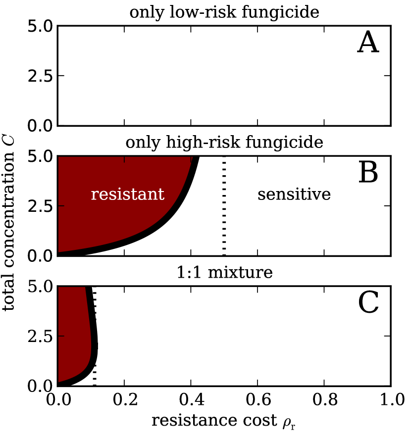
The ranges of fungicide dose and cost of resistance at which the sensitive (white) or resistant (grey) pathogen strain is favored by selection are shown in Fig. 2. In all scenarios competitive exclusion is observed: one of the strains takes over the whole pathogen population and the other one is eliminated. If a low-risk fungicide is applied alone, the sensitive strain has a selective advantage across the whole parameter range in Fig. 2A. When only a high-risk fungicide is applied (Fig. 2B) the resistance dominates if the fitness cost is lower than the maximum effect of the fungicide and at a fungicide dose higher than a threshold value which increases with the fitness cost (solid curve in Fig. 2B). If the fitness cost exceeds (dotted line in Fig. 2B), then the sensitive strain dominates at any fungicide dose. The Fig. 2C shows the outcome when the two fungicides are mixed at equal concentrations. Here the fitness cost at which the sensitive strain dominates is reduced (vertical dotted line is shifted to the left).
As expected, without a fitness cost () the resistant strain becomes favored by selection and will eventually dominate the population whenever the high-risk fungicide is applied, alone or in combination with the low-risk fungicide (Fig. 2B,C).
2.2 Optimal proportion of fungicides in a mixture
It is highly desirable to keep existing fungicides effective for as long as possible. From this point of view, an optimal mixture contains the largest proportion of the high-risk fungicide, at which (i) the resistant pathogen strain is not selected and (ii) an adequate level of disease control is achieved. In order to fulfill both of these objectives, the fitness cost of resistance needs to be larger than a threshold value [see Eq. (A.16)]. The threshold is shown by the dotted vertical line in Fig. 2C.
The threshold depends on the proportion of fungicides in the mixture. Adding more of the low-risk fungicide, while keeping the same total dose , reduces the threshold. This diminishes the range of the values for fitness cost over which the resistant strain dominates. On the other hand, adding less of the low-risk fungicide, while again keeping the same, increases the threshold, which increases the parameter range over which the resistant strain is favored.
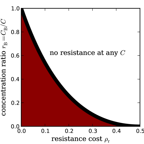
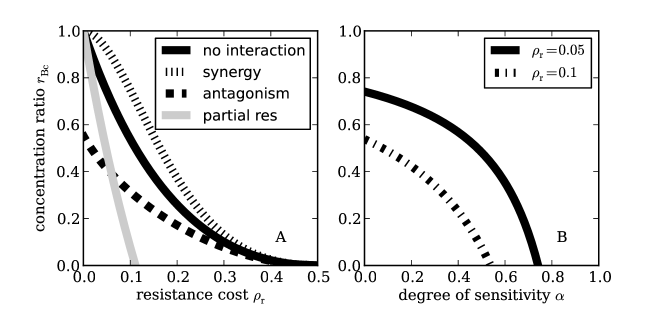
Therefore, at a given fitness cost , one can adjust the fungicide ratio such that . This is shown in Fig. 3: the curve shows the critical proportion of the low-risk fungicide , above which no selection for resistance occurs at any total fungicide dose . One can see from Fig. 3 that if the resistance cost is absent (), then the high-risk fungicide should not be added at all if one wants to prevent selection for resistance. At larger fitness costs, the value of decreases, giving the possibility to use a larger proportion of the high-risk fungicide without selecting for resistance.
Finding an optimum proportion of fungicides requires knowledge of both the fitness cost and the maximum effect of the fungicide [Eq. (A.17)]. However, if the cost of resistance and fungicides affect the infectious period of the pathogen (see Sec. A.5) and not the transmission rate as we assumed above, then a simpler expression for the critical proportion of fungicides in the mixture is obtained [Eq. (A.18)], which depends only on the ratio between the fitness cost and the maximum fungicide effect . In this case, if the fitness cost is at least 5 percent of the maximum fungicide effect, then we predict that up to about 20 percent of the high-risk fungicide can be used in a mixture without selecting for resistance. An example of the cost of fungicide resistance manifesting as a reduction in infectious period was in metalaxyl-resistant isolates of Phytophthora infestans [29]. In this experiment, the infectious period of the resistant isolates was reduced, on average, by 25 % compared to the susceptible isolates [29].
So far we have shown how choosing an optimal proportion of fungicides in the mixture prevents selection for resistance. Now, we will consider in more detail how to achieve an adequate level of disease control.
2.3 Treatment benefit
The yield of cereal crops is usually assumed to be proportional to the healthy green leaf area, which corresponds in our model to the amount of healthy hosts . Accordingly, we quantify the benefit of the fungicide treatment, , as the ratio between the amount of healthy hosts when both the disease and treatment are present and its value in the absence of disease: . Hence, corresponds to a perfect treatment, which eradicates the disease completely and the treatment benefit of zero corresponds to a situation where all healthy hosts are infected by disease. In order to obtain analytical expressions for the treatment benefit , we consider one growing season and assume that the host-pathogen equilibrium is reached during the season (see Appendix A.3 for a discussion of these assumptions).
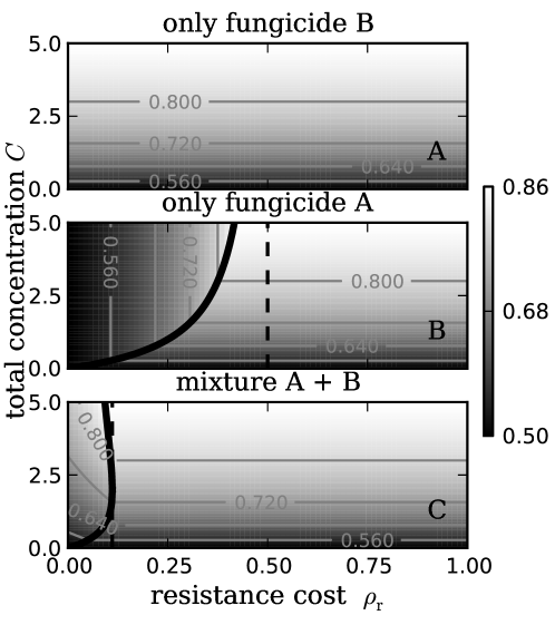
The treatment benefit at equilibrium is shown in Fig. 4 as a function of the fitness cost and the fungicide dose (see Appendix A.3 for equations). When a low-risk fungicide is applied alone [Fig. 4A], the sensitive strain is favored by selection over the whole range of parameters. Therefore, the treatment benefit increases monotonically with the fungicide dose and is not affected by the cost of resistance. In contrast, when a high-risk fungicide is applied alone [Fig. 4B], a region at low fitness costs appears [to the left from the solid curve in Fig. 4B], where the resistant strain is favored. Here, the treatment benefit does not depend on the fungicide dose, but increases with the cost of resistance. Hence, if the fitness cost is too low to stop selection for resistance, then the fungicide treatment will fail.
In the case of a mixture of a high-risk and a low-risk fungicide, the parameter range over which the resistant strain is favored becomes smaller [Fig. 4C, to the left from the solid curve]. In this range the treatment benefit increases with the cost of resistance, since larger costs reduce the impact of disease per se. Also, the treatment benefit increases with the total fungicide dose in this range, because the low-risk fungicide works against the resistant strain.
As we have shown above in Sec. 2.2, in the presence of a substantial fitness cost, one can avoid selection for resistance by adjusting the proportion of the two fungicides in the mixture. Then, the total fungicide dose such that the treatment benefit reaches a high enough value and an adequate disease control is achieved.
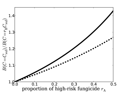
In the end of Sec. 2.2 we estimated that up to about 20 percent of the high-risk fungicide can be used in a mixture without selecting for resistance if the fitness cost is at least 5 percent of the maximum fungicide effect on the infectious period . But how much extra control does one obtain by adding the high-risk fungicide to the mixture? We estimate that adding 20 percent of the high-risk fungicide to the mixture increases the treatment benefit by about 12 percent at and by about 9 percent at (see Sec. A.3 and Fig. A.1 for more details). In the case when the high-risk fungicide has a larger maximum effect, i. e. , the benefit of adding it to the mixture will increase. However, the largest proportion of the high-risk that can be added without selecting for resistance will decrease.
2.4 The effect of pharmacological interaction between fungicides
Synergistic interactions between fungicides make their combined effect greater than expected with additive interactions. The sensitive pathogen strain is suppressed more by a synergistic mixture, while the resistant strain is not affected by the interaction (in case of full resistance ). This increases the range of fitness costs over which resistance has a selective advantage [the dashed line in Fig. 2C shifts to the right]. Consequently, the critical proportion of the low-risk fungicide in the mixture , above which the resistant mutants are eliminated increases [dotted curve in Fig. 5A]. In contrast, an antagonistic mixture suppresses the sensitive strain less effectively than either fungicide used alone. In this case the range of fitness costs over which resistance dominates becomes smaller and the ratio decreases [dashed curve in Fig. 5A]. Hence, reduced resistance evolution is achieved, however, at the expense of reduced disease control. This result is in agreement with studies on drug interactions in the context of antibiotic resistance, where antagonistic drug combinations were found to select against resistant bacterial strains [12].
2.5 The effect of partial fungicide resistance
Consider the situation when the resistant pathogen strain is not fully protected from the high-risk fungicide, but exhibits a partial resistance (). In this case, the fungicide mixture is more effective in suppressing the resistant strain than in the case of full resistance () considered above. Therefore, one needs less of the low-risk fungicide in the mixture to reach the conditions where resistance is eliminated by selection: the critical proportion of the low-risk fungicide in the mixture decreases with the degree of sensitivity in Fig. 5B. Also, in Fig. 5A the dependency of the critical ratio of the fungicide B in the mixture for partial resistance (light grey curve) lies below the one at perfect resistance and reaches zero at a much smaller value. Thus, knowledge of the degree of resistance is crucial for determining an appropriate proportion of fungicides in the mixture.
3 Discussion
The three main outcomes of our study are: (i) if fungicide resistance comes without a fitness cost, application of fungicides prone to resistance (high-risk fungicides) in a mixture with fungicides still free from resistance (low-risk fungicides) will select for resistance; (ii) if sufficiently high costs are found, then an optimal proportion of the high-risk fungicide in a mixture with the low-risk fungicide exists that does not select for resistance; (iii) this mixture can potentially be used for preventing de novo emergence of fungicide resistance, in which case the relevant fitness cost is the “inherent” cost of fungicide resistance before the compensatory evolution occurs (see below).
In the absence of fitness costs application of a mixture of high-risk and low-risk fungicides will select for resistance. Consequently, the resistant strain will eventually dominate the pathogen population and the sensitive strain will be eliminated. Because of this, the high-risk fungicide will not affect the amount of disease and only the low-risk fungicide component of the mixture will be acting against disease. Hence, the high-risk fungicide becomes nonfunctional in the mixture and using the low-risk fungicide alone would have the same effect at a lower financial and environmental cost.
In contrast, if sufficiently high costs are found, then high-risk fungicides can be used effectively for an extended period of time. According to our model, an optimal proportion of the high-risk fungicide in a mixture with the low-risk fungicide can be determined that contains as much as possible of the high-risk fungicide, but still does not select for resistance while providing adequate disease control (see Box 1). If a mixture with the optimum proportion is applied, then the rise of the resistant strain is prevented for an unlimited time. Thus, the scheme in Box 1 provides a framework for using our knowledge about the evolutionary dynamics of plant pathogens and their interaction with fungicides in devising practical strategies for management of fungicide resistance.
In order to apply the scheme in Box 1, one needs to know dose-response parameters of the fungicides and , the degree of fungicide sensitivity (or the resistance factor), the degree of pharmacological interaction and the fitness cost of resistane mutations. Fungicide dose-response curves are routinely determined empirically (for example, [36, 43]) and can be used to estimate the model parameters and [22]. The fungicide sensitivity is known to be lost completely in some cases (for example, most cases of QoI resistance), i. e. , while in other cases with partial resistance the degree of sensitivity (or the resistance factor) was measured (for example, [33]). Pharmacological interaction between several different fungicides was also characterized empirically (see [16] and the references therein). Also, the fitness costs of resistance were characterized empirically in many cases (see below). In the past these measurements were performed independently, but our study provides motivation to bring them together, since all these parameters need to be characterized for the same plant-pathogen-fungicide combination.
These measurements will allow one to predict the optimal proportion of the two fungicides in the mixture theoretically. This prediction needs to be tested using field experimentation, in which the amount of disease and the frequency of resistance would be measured as functions of time at different proportions of the high- and low-risk fungicides in the mixture. From these measurements the optimal proportion of the fungicides can be obtained empirically. It is this empirically determined optimal proportion of fungicides that can be used for practical guidance on management of fungicide resistance. Moreover, from the comparison of the optimal proportion obtained theoretically and empirically, one can evaluate the performance of the model and identify the aspects of the model that need improvement.
So far we considered the scenario where both the sensitive and the resistant pathogen strains increase from low numbers, i. e. resistant mutants pre-exist in the pathogen population. In this scenario the strain with higher fitness (or basic reproductive number) eventually outcompetes the other strain. This competition may occur over a time scale of several growing seasons so that there is enough time for compensatory mutations that diminish fitness costs of resistance to emerge. This needs to be taken into account when determining the optimal proportion of fungicides in the mixture. However, an alternative scenario is possible when resistant mutants emerge de novo through mutation or migration and, in order to survive, they need to invade the host population already infected by the sensitive strain. The threshold of invasion in this case depends on the “inherent” fitness cost of resistance mutations, i. e. their cost before the compensatory evolution occurs. In this case, one should measure the “inherent” cost of resistance mutations when performing step 3 in Box 1.
As discussed above, it is crucial to know fitness costs of resistance mutations in order to determine whether the fungicide mixture will select for resistance. We extensively searched the literature on fitness costs in different fungal pathogens of plants. A few studies inferred substantial fitness costs from field monitoring (see for example, [53] and references in [44]). But these findings could result from other factors, including immigration of sensitive isolates, selection for other traits linked to resistance mutations or genetic drift [44]. Though relatively few carefully controlled experiments have been conducted, the majority indicate that fitness costs associated with fungicide resistance are either low (for example, [8, 32]) or absent (for example, [14, 45]). But in some cases fitness costs were found to be substantial (for example, [26, 31, 25, 55]) both in laboratory measurements and in field experiments. Although measurements of fitness costs of resistant mutants performed under laboratory conditions can be informative (as, for example in [8]), they do not necessarily reflect the costs connected with resistant mutants selected in the field. This is because field mutants are likely to possess compensatory mutations improving pathogen fitness [44]. Moreover, a laboratory setting rarely reflects the balance of environmental and host conditions found throughout the pathogen life-cycle, since the field environment is much more complex.
However, the most relevant measure of pathogen fitness in the context of our study is the growth rate of the pathogen population at the very beginning of an epidemic (often denoted as ). It is directly related to the basic reproductive number . To the best of our knowledge, the fitness costs of fungicide resistant strains were not measured with respect to . In the studies cited above different components of fitness were measured that may or may not be related to . Therefore, we identified a major gap in our knowledge of fitness costs. We hope this study will stimulate further experimental investigations to better characterize fitness costs and expect that substantial costs will be found in some cases.
Interactions of plants with fungal pathogens, fungicide action and, possibly, pharmacological interaction can depend on environmental conditions. This means that the outcomes of measurements necessary for applying the scheme in Box 1, may vary between seasons and geographical locations. Moreover, the outcomes may also be different in different host cultivars. Therefore, the optimal proportion of fungicides in the mixture may vary between seasons, geographical locations and host cultivars. Thus, to provide general practical guidance on management of fungicide resistance, one needs to measure the optimal proportion of fungicides over many seasons, in different geographical locations and host cultivars. This difficulty is not a unique property of our study, but rather it is a general problem in the field of mathematical modeling of fungicide resistance and plant diseases. For example, it is also relevant for choosing appropriate fungicide dose rate [36].
While it was previously discussed [51] that alternation of high-risk and low-risk fungicides might be a useful tactic for disease control in the presence of a fitness cost, we have shown that a mixture of these fungicides in an appropriate proportion can provide adequate disease control without selecting for resistance. Mixtures offer an advantage compared to alternation because there is no need to delay the application of the high-risk fungicide and the resistant strain does not rise to high frequencies, which lowers the risk of its further spread (see Appendix A.6).
According to our model, one can avoid selection for resistance while providing adequate disease control by choosing the fungicide ratio and the total dose in the following way:
-
1.
measure the pharmacological properties of both fungicides under field conditions to determine , and ;
-
2.
determine the degree of fungicide sensitivity under field conditions;
-
3.
determine the degree of pharmacological interaction between fungicides A and B under field conditions;
-
4.
measure the fitness cost of resistance under field conditions;
-
5.
choose the proportion of the fungicide B above the threshold: , such that the resistance is not favored by selection at any total fungicide dose ;
-
6.
choose the total fungicide dose, which should be large enough to achieve an adequate level of disease control (see Fig. 4C).
The problem of combining chemical biocides in order to delay or prevent the development of resistance also appears in other contexts, including resistance of agricultural weeds to herbicides [5] and insect pests to insecticides [47]. The fitness cost of resistance is also recognized as a crucial parameter for managing antibiotic resistance [3].
Development of mathematical models of fungicide resistance dynamics has been influenced by theoretical insights from animal and human epidemiology [11, 20]. Similarly, we expect that lessons learned from modeling fungicide combinations may well apply to the problem of biocide resistance in the other contexts. In particular, one can investigate the idea of adjusting the proportion of the components in a mixture of drugs in order to prevent selection for resistance in a more general context of biocide resistance.
Acknowledgements
AM and SB gratefully acknowledge support by the European Research Council advanced grant PBDR 268540. The authors are grateful to Michael Milgroom and Michael Shaw for helpful comments concerning fitness costs of fungicide resistance and to two anonymous reviewers for improving the manuscript.
References
- [1] Abbott, W., 1925. A method of computing the effectiveness of an insecticide. Journal of economic entomology 18:265.
- [2] Anderson, R. M. and May, R. M., 1986. The invasion, persistence and spread of infectious diseases within animal and plant communities. Philosophical transactions of the Royal Society of London. Series B, Biological sciences 314:533–70.
- [3] Andersson, D. I. and Hughes, D., 2010. Antibiotic resistance and its cost: is it possible to reverse resistance? Nature Reviews Microbiology 8:260–271.
- [4] Austin, D. J. and Anderson, R. M., 1999. Studies of antibiotic resistance within the patient, hospitals and the community using simple mathematical models. Philosophical transactions of the Royal Society of London. Series B, Biological sciences 354:721–38.
- [5] Beckie, H. J. and Reboud, X., 2009. Selecting for weed resistance: herbicide rotation and mixture. Weed Technology 23:363–370.
- [6] Bell, G. and Gonzalez, A., 2011. Adaptation and evolutionary rescue in metapopulations experiencing environmental deterioration. Science 332:1327–30.
- [7] Berenbaum, M., 1989. What is synergy? Pharmacological Reviews 41:93.
- [8] Billard, A., Fillinger, S., Leroux, P., Lachaise, H., Beffa, R., and Debieu, D., 2012. Strong resistance to the fungicide fenhexamid entails a fitness cost in Botrytis cinerea, as shown by comparisons of isogenic strains. Pest management science 68:684–91.
- [9] Bliss, C. I., 1939. The toxicity of poisons applied jointly. Annals of Applied Biology 26:585–615.
- [10] Bonten, M. J. M., Austin, D. J., and Lipsitch, M., 2001. Understanding the Spread of Antibiotic Resistant Pathogens in Hospitals : Mathematical Models as Tools for Control. Healthcare Epidemiology 33:1739–1746.
- [11] van den Bosch, F. and Gilligan, C. A., 2008. Models of fungicide resistance dynamics. Annu. Rev. Phytopathol. 46:123–47.
- [12] Chait, R., Craney, A., and Kishony, R., 2007. Antibiotic interactions that select against resistance. Nature 446:668–71.
- [13] Cools, H. J., 2008. Are azole fungicides losing ground against Septoria wheat disease? Resistance mechanisms in Mycosphaerella graminicola. Pest Manag. Sci. 64:681–684.
- [14] Corio-Costet, M.-F., Dufour, M.-C., Cigna, J., Abadie, P., and Chen, W.-J., 2010. Diversity and fitness of Plasmopara viticola isolates resistant to QoI fungicides. European Journal of Plant Pathology 129:315–329.
- [15] Fernández-Ortuño, D., Torés, J. A., Vicente, A. D., and Pérez-García, A., 2008. Mechanisms of resistance to QoI fungicides in phytopathogenic fungi. International Microbiology 11:1–9.
- [16] Gisi, U., 1996. Synergistic interaction of fungicides in mixtures. Phytopathology 86:1273.
- [17] Gisi, U., Sierotzki, H., Cook, A., and McCaffery, A., 2002. Mechanisms influencing the evolution of resistance to Qo inhibitor fungicides. Pest management science 58:859–67.
- [18] Greco, W. and Bravo, G., 1995. The search for synergy: a critical review from a response surface perspective. Pharmacological Reviews 47:331.
- [19] Gubbins, S. and Gilligan, C. A., 1999. Invasion Thresholds for Fungicide Resistance: Deterministic and Stochastic Analyses. Proc. R. Soc. Lond. B 266:pp. 2539–2549.
- [20] Hall, R. J., Gubbins, S., and Gilligan, C. A., 2004. Invasion of drug and pesticide resistance is determined by a trade-off between treatment efficacy and relative fitness. Bulletin of mathematical biology 66:825–40.
- [21] Hall, R. J., Gubbins, S., and Gilligan, C. A., 2007. Evaluating the performance of chemical control in the presence of resistant pathogens. Bulletin of mathematical biology 69:525–37.
- [22] Hobbelen, P. H. F., Paveley, N. D., and van den Bosch, F., 2011. Delaying selection for fungicide insensitivity by mixing fungicides at a low and high risk of resistance development: a modeling analysis. Phytopathology 101:1224–33.
- [23] Hobbelen, P. H. F., Paveley, N. D., Oliver, R. P., and van den Bosch, F., 2013. The Usefulness of Fungicide Mixtures and Alternation for Delaying the Selection for Resistance in Populations of Mycosphaerella graminicola on Winter Wheat: A Modeling Analysis. Phytopathology 103:690–707.
- [24] Hoffmann, A. A. and Sgrò, C. M., 2011. Climate change and evolutionary adaptation. Nature 470:479–85.
- [25] Holmes, G. and Eckert, J., 1995. Relative fitness of imazalil-resistant and-sensitive biotypes of Penicillium digitatum. Plant disease 79:1068–1073.
- [26] Iacomi-Vasilescu, B., Bataille-Simoneau, N., Campion, C., Dongo, A., Laurent, E., Serandat, I., Hamon, B., and Simoneau, P., 2008. Effect of null mutations in the AbNIK1 gene on saprophytic and parasitic fitness of Alternaria brassicicola isolates highly resistant to dicarboximide fungicides. Plant Pathology 57:937–947.
- [27] Josepovits, G. and Dobrovolszky, A., 1985. A novel mathematical approach to the prevention of fungicide resistance. Pesticide Science 16:17–22.
- [28] Kable, P. and Jeffery, H., 1980. Selection for Tolerance in Organisms Exposed to Sprays of Biocide Mixtures: A Theoretical Model. Phytopathology 79:8–12.
- [29] Kadish, D. and Cohen, Y., 1989. Population dynamics of metalaxyl-sensitive and metalaxyl-resistant isolates of Phytophthora infestans in untreated crops of potato. Plant Pathology 38:271–276.
- [30] Kadish, D. and Cohen, Y., 1992. Overseasoning of metalaxyl-sensitive and metalaxyl-resistant isolates of Phytophthora infestans in potato tubers weeks after inoculation. Phytopathology 82:887–889.
- [31] Karaoglanidis, G., Thanassoulopoulos, C., and Ioannidis, P., 2001. Fitness of Cercospora beticola field isolates–resistant and–sensitive to demethylation inhibitor fungicides. European Journal of Plant Pathology 107:337–347.
- [32] Kim, Y. K. and Xiao, C. L., 2011. Stability and fitness of pyraclostrobin- and boscalid-resistant phenotypes in field isolates of Botrytis cinerea from apple. Phytopathology 101:1385–91.
- [33] Leroux, P., Albertini, C., Gautier, A., Gredt, M., and Walker, A.-S., 2007. Mutations in the CYP51 gene correlated with changes in sensitivity to sterol 14-demethylation inhibitors in field isolates of Mycosphaerella graminicola. Pest Management Science 63:688–698.
- [34] Levin, B. R., 2001. Minimizing Potential Resistance: A Population Dynamics View. Clinical Infectious Diseases 33:161–169.
- [35] Levy, Y., Benderly, M., Cohen, Y., Gisi, U., and Bassand, D., 1986. Joint action of fungicides in mixtures: comparison of two methods for synergy calculation. EPPO Bulletin 16:651–657.
- [36] Lockley, D. and Clark, W., 2005. Fungicide dose-response trials in wheat: the basis for choosing ”appropriate dose”. Home-Grown Cereals Authority, UK, Project Report 373.
- [37] Milgroom, M. G., Levin, S. A., and Fry, W. E., 1989. Population genetics theory and fungicide resistance. In Leonard, K. J. and Fry, W. E., eds., Plant Disease Epidemiology. 2. Genetics, resistance and management, 340–367, McGraw Hill, New York.
- [38] Mullins, J. G. L., Parker, J. E., Cools, H. J., Togawa, R. C., Lucas, J. a., Fraaije, B. a., Kelly, D. E., and Kelly, S. L., 2011. Molecular modelling of the emergence of azole resistance in Mycosphaerella graminicola. PloS one 6:e20973.
- [39] Orton, E. S., Deller, S., and Brown, J. K. M., 2011. Pathogen profile update Mycosphaerella graminicola: from genomics to disease control. Molecular Plant Pathology 12:413–424.
- [40] Ozcaglar, C., Shabbeer, A., Vandenberg, S. L., Yener, B., and Bennett, K. P., 2012. Epidemiological models of Mycobacterium tuberculosis complex infections. Mathematical biosciences 236:77–96.
- [41] Palmer, C. and Skinner, W., 2002. Mycosphaerella graminicola: latent infection, crop devastation and genomics. Molecular plant pathology 3:63–70.
- [42] Parnell, S., Gilligan, C. a., and van den Bosch, F., 2005. Small-scale fungicide spray heterogeneity and the coexistence of resistant and sensitive pathogen strains. Phytopathology 95:632–9.
- [43] Paveley, N., Hims, M., and Stevens, D., 1998. Appropriate fungicide doses for winter wheat and matching crop management to growth and yield potential. Home-Grown Cereals Authority, UK, Project Report 166.
- [44] Peever, T. and Milgroom, M., 1995. Fungicide resistance - lessons for herbicide resistance management? Weed technology 9:840.
- [45] Peever, T. L. and Milgroom, M. G., 1994. Lack of correlation between fitness and resistance to sterol biosynthesis-inhibiting fungicides in Pyrenophora teres. Phytopathology 84:515.
- [46] Pfender, W., 2006. Interaction of Fungicide Physical Modes of Action and Plant Phenology in Control of Stem Rust of Perennial Ryegrass Grown for Seed. Plant disease 90:1225.
- [47] Roush, R., 2006. Designing resistance management programs: how can you choose? Pesticide Science 26:15–16.
- [48] Shaw, M., 1989. Independent action of fungicides and its consequences for strategies to retard the evolution of fungicide resistance. Crop Protection 8:405–411.
- [49] Shaw, M., 1993. Theoretical analysis of the effect of interacting activities on the rate of selection for combined resistance to fungicide mixtures. Crop Protection 12:120–126.
- [50] Shaw, M. W., 1989. A model of the evolution of polygenically controlled fungicide resistance. Plant Pathology 38:44–55.
- [51] Shaw, M. W., 2006. Is there such a thing as a fungicide resistance strategy? A modeller’s perspective. Aspects of Applied Biology 78:37–43.
- [52] Skylakakis, G., 1981. Effects of alternating and mixing pesticides on the buildup of fungal resistance. Phytopathology 71:1119.
- [53] Suzuki, F., Yamaguchi, J., and Koba, A., 2010. Changes in fungicide resistance frequency and population structure of Pyricularia oryzae after discontinuance of MBI-D fungicides. Plant Disease 94:329–334.
- [54] Torriani, S. F., Brunner, P. C., McDonald, B. A., and Sierotzki, H., 2009. QoI resistance emerged independently at least 4 times in European populations of Mycosphaerella graminicola. Pest Manag. Sci. 65:155–62.
- [55] Webber, J., 1988. Effect of MBC fungicide tolerance on the fitness of Ophiostoma ulmi. Plant pathology 37:217–224.
- [56] Wong, F. and Wilcox, W., 2001. Comparative physical modes of action of azoxystrobin, mancozeb, and metalaxyl against Plasmopara viticola (grapevine downy mildew). Plant Disease 85:649–656.
- [57] Zhan, J., Stefanato, F., and McDonald, B., 2006. Selection for increased cyproconazole tolerance in Mycosphaerella graminicola through local adaptation and in response to host. Molecular plant pathology 7:259–268.
Appendix A Supplemental materials
A.1 Model equations
In order to explore the effect of the assumptions we made in Sec. 1, we consider a more general system of equations, which describes the change in time of the same quantities as in Eqs. (1)-(3): the amount of healthy host tissue , the amount of host tissue infected with the sensitive pathogen strain and the amount of host tissue infected with the resistant pathogen strain
| (A.1) | ||||
| (A.2) | ||||
| (A.3) |
where, the function describes the effect of the application of the mixture fungicides A and B with doses and on the transmission rate of the sensitive pathogen strain and the function describes the effect of this mixture on the transmission rate of the resistant strain:
| (A.4) | ||||
| (A.5) |
The parameters , , and characterize the degree of sensitivity of each of the two pathogen strains (index ”s” for the sensitive strain, index “r” for the resistant strain) to each of the two fungicides A and B. Their values are between zero and one. In this general case both pathogen strains are partially resistant to both fungicides. The maximum effect of the fungicide is characterized by the parameter and assumed to be the same for both fungicides.
The parameter in Eqs. (A.4), (A.5) is modified due to pharmacological interaction between fungicides characterized by the degree of interaction . At fungicides do not interact, represents synergy and corresponds to antagonism. [We restrict our consideration to , since otherwise the term in the square brackets of Eqs. (A.4), (A.5) may become negative, which makes no sense.] This way to define pharmacological interaction between compounds is called “Loewe additivity” or “concentration addition” in the literature [18, 7]. In this approach an interaction of a compound with itself is set by definition to be additive (zero interaction). For example, when the fungicide A is mixed with itself, the resulting sham mixture is neither synergistic, nor antagonistic but has zero interaction. An equivalent graphic procedure is known as the Wadley method in the fungicide literature [second method described in [35]].
An alternative way to define pharmacological interaction assumes that the two compounds have independent modes of action and is called “Bliss independence” [9] or Abbott’s formula [1]. However, in this definition a compound can have a pharmacological interaction with itself, i. e. be synergistic or antagonistic. The study [48] discusses the definition of “independent action” of the two fungicides, according to which the two fungicides are independent when one fungicide does not affect the evolution of resistance in the other. According to [48, 49], this is only possible when each of the fungicides affects different stages of the pathogen life cycle.
There are several ways to introduce a deviation from the zero interaction regime, in which usually an interaction term is added to the isobologram equation [18]. We have chosen a specific form of the interaction term, which is proportional to the square root of the product of the concentrations of the two compounds [Eq. (28) in [18]]. This form allows for a simple analytical expression of the effect of the combination in Eqs. (A.4), (A.5).
We assume that the cost of resistance decreases the transmission rate by a fixed amount for the sensitive strain and by for the resistant strain in Eqs. (A.1)-(A.3). We restrict our consideration here to the case when the “sensitive” pathogen strain is fully sensitive to both fungicides () and the “resistant” strain can have varying degrees of resistance to the fungicide A (, ), but is fully sensitive to the fungicide B (). Therefore, the cost of resistance for the sensitive strain is zero . Then, the fungicide dose-response functions become simpler.
In order to determine the range of fitness costs and fungicide doses , over which the sensitive or resistant strain is favored by selection, we perform the linear stability analysis of the fixed points of the system Eqs. (A.1)-(A.3). Fixed points are the values of , and at which the expressions on the right-hand side of Eqs. (A.1)-(A.3) equal zero. The system Eqs. (A.1)-(A.3) has three fixed points: (i) , ; (ii) , , ; (iii) , , . Here , . To determine whether a fixed point is stable, we first linearize the system Eqs. (A.1)-(A.3) in its vicinity, then determine the Jacobian and its eigenvalues. A fixed point is stable if all the eigenvalues have negative real parts.
The results of this analysis can be conveniently expressed using the basic reproductive number of the sensitive strain
| (A.6) |
and the basic reproductive number of the resistant strain
| (A.7) |
The sensitive strain is favored by selection [meaning that the fixed point (ii) is stable and both fixed points (i) and (iii) are unstable] when both inequalities , are fulfilled.
We consider then the inequality , which is equivalent to
| (A.8) |
where
| (A.9) |
| (A.10) |
and is the proportion of the funcigide B in the mixture, .
The inequality (A.8) holds at
| (A.11) |
or at
| (A.12) |
Here,
| (A.13) |
| (A.14) |
where
| (A.15) |
According to the inequality (A.12), if the fitness cost of resistance is larger than a threshold value given by Eq. (A.13), the sensitive strain has a selective advantage and the resistant strain is eliminated from the population at any fungicide dose .
For the case of no interaction between fungicides () and perfect resistance () we obtain from Eq. (A.9) and Eq. (A.10) , . Then, the Eq. (A.13) is simplified:
| (A.16) |
We then solve the inequality with respect to and find that it is fulfilled at , where
| (A.17) |
It represents the critical proportion of the fungicide B in the mixture above which the resistant strain is not favored by selection (Fig. 3). If the cost of resistance affects the death rate of the pathogen (see Sec. A.5) and not the transmission rate as considered above, then a simpler expression for the critical proportion of the fungicide B is obtained
| (A.18) |
Here, depends only on the ratio of the cost of resistance to the maximum fungicide effect , which allows to make a more general prediction about the value of .
A.2 Selection for resistance at no interaction between fungicides
When only the high risk fungicide (fungicide A) is applied with the dose , we set in Eq. (A.9) and Eq. (A.10) to obtain , . Then, the following expressions are obtained for the threshold value of the resistance cost from Eq. (A.13)
| (A.19) |
and the fungicide dose from Eq. (A.14)
| (A.20) |
where
| (A.21) |
In the simpler case of full resistance we take the limit . Then, by taking this limit in Eq. (A.19), Eq. (A.20) and Eq. (A.21) we obtain for the threshold values of the fitness cost and the fungicide dose
| (A.22) |
| (A.23) |
In this case the sensitive strain dominates at if or at any positive values of if [white area in Fig. 2B].
When only the low risk fungicide (fungicide B) is applied, we set and, hence in the inequality (A.8) and obtain
| (A.24) |
This inequality holds and the sensitive strain dominates for all positive values of and at which .
Consider the case when the two fungicides A and B are applied together at an arbitrary mixing ratio , assuming no pharmacological interaction () and perfect resistance of the resistant strain to the fungicide A (). In this case, and . Substituting these values in Eq. (A.13), Eq. (A.14) and Eq. (A.15) gives the same expressions as in Eq. (A.19), Eq. (A.20) and Eq. (A.21), but with substituted by .
A.3 Expressions for the treatment benefit
The treatment benefit is defined as the ratio between the amount of healthy hosts when both the disease and treatment are present and the amount of healthy hosts at no disease (see Sec. 2.3).
In order to obtain analytical expressions for , we consider one growing season and assume the host-pathogen equilibrium is reached during the season. This corresponds to the time-dependent solution of Eqs. (1)-(3) reaching its stable fixed point (or steady state). Fixed points of Eqs. (1)-(3) can be found by equating the right-hand sides of all equations to zero and solving the resulting algebraic equations with respect to , and . Biologically this occurs when the first positive term in Eq. (1) corresponding to growth of healthy hosts, is compensated by the second, negative term that corresponds to the decrease in healthy hosts due to infection. In other words, equilibrium occurs when the rate of emergence of new healthy tissue as a result of plant growth is exactly offset by the rate of its decrease due to infection. The right-hand side of Eq. (2) goes to zero, when the rate of increase in due to new infections is compensated by the loss of the infectious tissue due to the completion of the infectious period (similar reasoning applies for Eq. (3)).
Then, the treatment benefit is given by
| (A.25) |
where is the equilibrium amount of healthy hosts and is the host carrying capacity, and assume full resistance ().
When only the fungicide B is applied at a dose [Fig. 4A], the basic reproductive number of the sensitive pathogen strain always exceeds the one for the resistant strain . Therefore, the resistant mutants are eliminated in the long run and the amount of the healthy host tissue is equal to , where is given by Eq. (5). Then, according to Eq. (A.25), the treatment benefit is
| (A.26) |
It grows with the fungicide dose and saturates, since the function saturates.
Application of the fungicide A alone at a dose may favor either resistant or sensitive pathogen strain depending on the fitness cost of resistance and the fungicide dose [see Fig. 2B]. The treatment benefit in this case is
| (A.27) |
where the is given by Eq. (A.23).
Now, consider application of both fungicides in a mixture at equal concentrations (), assuming no interaction between fungicides (). In this case, again either resistant or sensitive pathogen strain will dominate the population depending on the fitness cost and the total fungicide dose [see Fig. 2C]. The treatment benefit now has the following expression
| (A.28) |
where , and and are given by Eq. (A.13) and Eq. (A.14) at , . The treatment benefit is shown as a function of the fungicide dose and the fitness cost of resistance in Fig. 4 for the three cases discussed above, according to Eqs. (A.26)-(A.28).
When a mixture of a high-risk and a low-risk fungicide is used with the total dose and the proportion of the low-risk fungicide , a relevant question arises: “How much additional control does the addition of the high-risk fungicide provide?”. In order to quantify the degree of additional control due the high-risk fungicide component of the mixture, we first set the sufficient level of control that needs to be achieved in terms of the treatment benefit (for example, we can set ). Then, we determine the dose of the fungicide mixture at which this level of control is achieved. We assume that the proportion of the two fungicides in the mixture was chosen such that , i. e. the sensitive pathogen strain is favored by selection. Hence, the the treatment benefit is given by [the upper expression in Eq. (A.28)]. We set and substitute the dependence of the pathogen infectious period or the transmission rate on the fungicide dose according to or . Then, we obtain
| (A.29) |
The ratio
| (A.30) |
characterizes the extra benefit due to addition of the high-risk fungicide, since is the treatment benefit when both high-risk and low-risk fungicides are present and is the treatment benefit when the high-risk fungicide is absent (here, is the proportion of the low-risk fungicide in the mixture). The ratio is shown in Fig. A.1 as a function of the proportion of the high-risk fungicide in the mixture . One sees from Fig. A.1 that the more high-risk fungicide is used in the mixture, the larger is the extra benefit from its application (provided that , when the sensitive pathogen strain is favored by selection). However, the largest which still does not favor the resistant strain is determined by the value of the fitness cost of fungicide resistance (see Sec. 2.2).
Interestingly, the ratio does not depend on where the fungicide acts, on the infectious period or the transmission rate , as long as the maximum fungicide effects in these to cases and are related by such that the basic reproductive number is reduced by the same amount when the maximum effect is achieved.
A.4 Dynamics of the frequency of the resistant pathogen strain
If the fungicide resistance is not associated with a fitness cost, then the resistant strain is favored by selection and eventually dominates the population whenever the high risk fungicide is applied alone or in a mixture with the low risk fungicide [Fig. 2B,C]. However, for a given value of the total fungicide dose , the selection for resistance slows down when applying the fungicide mixture as compared to the treatment with the high risk fungicide alone [as seen from time-dependent numerical solutions of the model Eqs. (1)-(3)] in agreement with the findings of [22].
In order to understand this result we consider the dynamics of the frequency of the resistant pathogen strain . The rate of its change is obtained from Eqs. (1)-(3) [37]
| (A.31) |
where
| (A.32) |
is the selection coefficient [a similar expression was found in [19]]. Here , and is the proportion of the fungicide B in the mixture. Here, , where the dose of the fungicide A and the dose of the fungicide B may depend on time due to fungicide decay:
| (A.33) |
where , are the fungicide doses at the time of application, and are the fungicide decay rates.
The expression (A.32) for the selection coefficient was obtained under the assumption that the fungicide decreases the transmission rate . In the case when the fungicide decreases the infectious period , the selection coefficient does not depend on the amount of healthy hosts .
Variables in Eq. (A.31) can be separated and a closed-form solution is found
| (A.34) |
One can see from Eq. (A.34) that the overall selection over the time is determined by the integral of the selection coefficient over time . We are interested in the overall selection that occurs during the time which is longer than the time scale of change in the fungicide dose. In this case, an equivalent, constant over time fungicide dose can be determined, which gives rise to the same value of the integral . This effective fungicide dose would take into account the time-dependent effect of the amount of the host tissue on the strength of selection.
Assuming a zero fitness cost (), no pharmacological interaction () and full resistance (), the selection coefficient can be written as
| (A.35) |
Assuming that is a slowly varying function compared to the time scale of selection, the solution of Eq. (A.31) reads:
| (A.36) |
where . At , the function grows monotonically and tends to one at large times. The rate, at which it grows is determined by the magnitude of the selection coefficient .
One can see from Eq. (A.35) that when the high risk fungicide is applied alone (), the selection coefficient is larger than when it is mixed with a low risk fungicide () at the same total fungicide dose . Hence, . This is because the function has positive values for any . Thus, the selection for the resistant strain (against the sensitive strain) is delayed when a mixture of high risk and low risk fungicides is applied compared to treatment with the high risk fungicide alone. A careful consideration of Eq. (A.34) reveals that this conclusion holds also when does not vary slowly over the time scale of selection. Lower fungicide dose will decrease the selection coefficient under the integral on the right-hand side of Eq. (A.34). Hence, in order to achieve a given large value of the frequency of resistance , one would need to integrate over a longer time .
A.5 Generalization of the model: effect of the fungicide and fitness cost of resistance on the pathogen
So far we assumed that both the resistance cost and fungicides affect the transmission rate . We performed the same analysis for the three remaining cases possible in the model: When (i) both resistance cost and the fungicide affect the pathogen death rate according to for the resistant strain and for the sensitive strain; (ii) the resistance cost affects the transmission rate of the resistant strain and the fungicides affect the pathogen death rate ; (iii) resistance cost affects the death rate of the resistant pathogen strain , while the fungicide affects the infection rate of both resistant and sensitive strains . We have found that although the mathematical expressions for the results have a different form in these cases and there is a slight quantitative difference, all the conclusions remain the same and do not depend on whether the fungicide and the resistance cost manifest in the infection rate or in the pathogen death rate .
Moreover, we have done the same analysis using a fungicide dose-response function different from Eq. (5), namely using the function . If the two fungicides have the same values of and and are applied at doses and , then according to Loewe’s additivity, their combined action has the form . We found again that all the conclusions remain the same in this case.
This generalization applies to determination of the direction of selection (the sign of the selection coefficient in Eq. (A.31)) and to the outcomes for the treatment benefit at equilibrium obtained in Sec. 2.3. However, the time-dependent solutions of Eqs. (1)-(3) may behave differently depending on how the fungicide and the fitness cost affect the pathogen life cycle and the form of the fungicide dose-response function. This is an interesting topic for further investigations, but lies beyond the scope of this study.
A.6 Fungicide mixture versus alternation
It was previously discussed [51] that in the presence of a fitness cost the alternation of fungicides can be effective, but we have shown here that fungicide mixtures can also be effective in this case. When using an alternation strategy, the period of selection during which the resistant strain is favored in the presence of the high risk fungicide is followed by a period during which selection favors the sensitive strain in the absence of this fungicide. The latter period is typically much longer because the selection pressure induced by the high risk fungicide is much larger than that induced by the fitness cost of resistance. Hence, one needs to wait for quite a long time before the resistant strain disappears and the high risk fungicide can be used again. Moreover, there are times during which the frequency of the resistant strain becomes large (at the end of the period of the application of the high risk fungicide), which increases the risk that resistance will spread to other regions. Both of these disadvantages are avoided by using a mixture where the proportion of the low risk fungicide is above a critical value determined here (Fig. 3). In this case there is no need to delay the application of the high risk fungicide and the frequency of the resistant strain does not rise above the mutation- or migration-selection equilibrium because the mixture does not induce selection for resistance.
A.7 The risk of double resistance
Although we do not consider the possibility of double resistance in our model, by applying an optimal proportion of fungicides in the mixture as suggested here, one would prevent selection for resistance to the high risk fungicide. Consequently, the risk of development of double resistance would be reduced. For both sexually and asexually reproducing pathogens, there are three pathways for generating double resistance: (i) A-resistant mutants are produced first and then a proportion of them acquires also B-resistance by spontaneous mutation (ii) B-resistant mutants are generated first and subsequently acquire A-resistance and (iii) double resistance is generated directly from the wild-type. In this case, by preventing selection for A-resistance, one removes only the pathway (i) to double resistance. If a pathogen is able to reproduce sexually, then a much more likely scenario for the double resistance to emerge is through recombination. For the recombination to occur, both singly resistant strains (A-resistant and B-resistant) would need to be present in the population at significant frequencies. Hence, preventing selection for A-resistance would diminish the probability of the emergence of double resistance by recombination. Thus, our findings would also help to significantly reduce the risk of development of double resistance, especially in sexually reproducing pathogens.