Mesoscopic Transport of Entangled and Nonentangled Kondo Singlets under Bias

Abstract

The unexplained tunneling conductances of correlated mesoscopic Kondo systems are understood by the coherent transport of the entangled and nonentangled singlets. Spins of the entangled singlet flow unidirectionally in a sequential up-and-down manner. This dynamics does not follow linear response theory. The side peaks at a finite bias are formed by resonant tunneling of the nonentangled singlet through a coherent tunneling level formed by two electron reservoirs within a coherent region. The theoretical line shapes remarkably fit the experimental data of a quantum point contact and a magnetized atom adsorbed on an insulating layer covering metallic substrate.

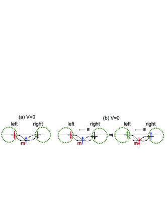
Figure 1: (Color online) (a) An entangled Kondo singlet at $V=0$. The dashed circle and the letter “m” denote the Kondo cloud and the mediating Kondo atom, respectively. (b) An entangled Kondo singlet at $V\approx 0$. Singlet hopping and partner changing leads to unidirectional spin flow. The horizontal arrow denotes the direction of the electric field.

The nonlinear line shapes of the tunneling conductance observed for mesoscopic Kondo systems are waiting for relevant theoretical explanations from the microscopic point of view. The two-reservoir Anderson impurity model at steady-state nonequilibrium is considered as a proper microscopic model describing a mesoscopic Kondo system. However, previous theoretical studies using the noncrossing approximation wingreen2 , the Keldysh formalism fujii , quantum Monte Carlo calculations han , and the extended numerical renormalization group method anders do not reproduce various nonlinear line shapes of mesoscopic Kondo systems. The difficulty originates from the combination of strong correlation and steady-state nonequilibrium. To solve this problem, we need to understand the dynamics under bias more clearly. It is obvious that the two-reservoir mesoscopic Kondo system at equilibrium has an entangled Kondo singlet represented by a wave function $|\Psi\rangle_{en}=p\!\!\mid\downarrow\uparrow\rangle_{LS}+q\!\!\mid\uparrow\downarrow\rangle_{LS}+u\!\!\mid\downarrow\uparrow\rangle_{RS}+v\!\!\mid\uparrow\downarrow\rangle_{RS}$, where $LS$ and $RS$ denote left singlet and right singlet, respectively and the coefficients are complex numbers, as shown in Fig. 1 (a). The equilibrium dynamics comprises multiple processes of exchange, partner change, and singlet hopping in a mixed manner among the four states given above. This complicated dynamics may be studied using the numerical renormalization group method for the low-energy regime wilson . Under bias, however, the dynamics becomes considerably simpler because the spins involved in the entanglement flow unidirectionally in an up-and-down sequence, as shown in Fig. 1 (b), until the entanglement is retained. The processes of singlet hopping and partner changing are used in the spin flow, and the coherent spins are provided from the Kondo cloud. The unidirectional flow does not allow a linear response regime. Backward motion of electrons may occur in the incoherent dynamics, and this leads to double occupancy at the mediating atom.

In this study, we clarify the spin dynamics forming the zero-bias peak and the side peaks and compare the theoretical results with the experimental data obtained for a quantum point contact sarkozy and an adsorbed magnetized atom on an insulating layer covering a metallic substrate otte , for example. Fitting the entire range of the line shapes of these systems is given for the first time.

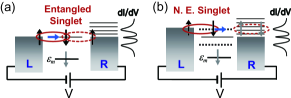
Figure 2: (Color online) (a) Transport of an entangled Kondo singlet at low bias. (b) Resonant tunneling of a nonentangled (N. E.) Kondo singlet through the coherent tunneling level (dashed line). $\varepsilon_{m}$ denotes the energy level of the mediating spin that forms a singlet.

In Fig. 2, we depict the low-energy tunneling schemes in the two-reservoir Anderson impurity model under bias along with the corresponding line shape of the tunneling conductance. Figure 2 (a) describes the transport near zero bias, i.e., $eV<k_{B}T_{K}$, where $e$, $V$, $k_{B}$, and $T_{K}$ denote the electron charge, source-drain bias, Boltzmann’s constant, and Kondo temperature for the entangled Kondo singlet, respectively. The unidirectional flow described in Fig. 1 (b) establishes the zero-bias peak in the tunneling conductance. The entanglement is completely broken when $eV>2k_{B}T_{K}$, in which a nonentangled Kondo singlet, $|\Psi\rangle_{ne}=p\!\!\mid\downarrow\uparrow\rangle_{LS}+q\!\!\mid\uparrow\downarrow\rangle_{LS}$, performs resonant tunneling and yields the side peak when it reaches the coherent transport channel shown by the dashed line in Fig. 2 (b). This transport also prohibits backward motion. Therefore, prohibiting backward motion of coherent spins is a generic feature of transport in a mesoscopic Kondo system under bias. This property significantly simplifies the dynamics at steady-state nonequilibrium. Another crucial feature is the existence of two coherent transport channels, shown in Fig. 2 (b), which is attributable to two reservoirs within the coherent region. Specific proof is given in a previous study hong11 and the basis vectors given later in the text clarify their existence. Previous studies wingreen2 ; fujii ; han ; anders have obtained a similar result showing Kondo peak splitting with bias. This phenomenon may occur when the two reservoirs are out of coherence. However, each of the aforementioned mesoscopic systems should be considered as a complete coherent system.

Now, we validate the tunneling mechanisms given in Fig. 2 by obtaining the tunneling conductance that fits the experimental result. The tunneling current of a mesoscopic system with an interacting site between two noninteracting reservoirs is given by haug

$$I=(e/\hbar)\int d\omega{\widetilde{\Gamma}}(\omega)[f_{L}(\omega)-f_{R}(\omega)]\rho^{ss}_{m}(\omega),$$

where $f_{L(R)}(\omega)$ is the Fermi distribution function of the left (or right) reservoir, ${\widetilde{\Gamma}}(\omega)=\Gamma^{L}(\omega)\Gamma^{R}(\omega)/[\Gamma^{L}(\omega)+\Gamma^{R}(\omega)]$, where $\Gamma^{L(R)}(\omega)=2\pi\sum_{k}|V_{km}^{L(R)}|^{2}\delta(\omega-\omega_{k})$ that involves the reservoir density of states, and $\rho^{ss}_{m}(\omega)$ is the local density of states (LDOS) at the mediating atom. The superscript $ss$ means steady-state nonequilibrium. This simplified form is derived from the well-known Meir-Wingreen current formula meir ; hersh by using the condition of the proportionate coupling function, $\Gamma^{L}(\omega)\propto\Gamma^{R}(\omega)$. This proportionate relation can be applicable to the elastic tunneling shown in Fig. 2. We employ a constant $\Gamma^{L,R}(\omega)$, indicating a flat density of states of metallic reservoirs.

Since the electrons in the singlet do not collide with a quasiparticle such as phonon until the bias excites it, $\rho^{ss}_{m}(\omega)$ in this study must be bias independent, i.e., $\partial\rho^{ss}_{m}(\omega)/\partial V=0$, which means one can write the tunneling conductance at zero temperature as

$$dI/dV=(e/\hbar){\widetilde{\Gamma}}(\omega)\rho^{ss}_{m}(\omega)|_{\hbar\omega=eV}.$$

The bias independence of $\rho^{ss}_{m}(\omega)$ will be retained unless inelastic tunneling is caused by the scattering with quasiparticles. In other studies on Kondo-involved mesoscopic systems wingreen ; schiller ; plihal , $\partial\rho^{ss}_{m}(\omega)/\partial V$ has also been neglected.

We obtain $\rho_{m\uparrow}^{ss}(\omega)$, which is given by $\rho_{m\uparrow}^{ss}(\omega)=-(1/\pi){\rm Im}[G^{+ss}_{mm\uparrow}(\omega)]$, by calculating the on-site retarded Green’s function, $iG^{+ss}_{mm\uparrow}(\omega)=\langle c_{m\uparrow}|(z+iL)^{-1}|c_{m\uparrow}\rangle$, where $z=-i\omega+0^{+}$, $c_{m\uparrow}$ is the fermion operator that annihilates an up-spin electron at the mediating atom and $L$ is the Liouville operator defined by $LA={\cal H}A-A{\cal H}$, in which ${\cal H}$ is the Hamiltonian and $A$ is an operator. To obtain $G^{+ss}_{mm\uparrow}(\omega)$ using the resolvent form, one needs a complete set of basis vectors spanning the Liouville space. We have obtained a complete set of orthonormal basis vectors hong11 ; hong10 describing $c_{m\uparrow}(t)$ that is driven by the Hamiltonian of the two-reservoir Anderson impurity model,

$${\cal H}={\cal H}_{0}^{L}+{\cal H}_{0}^{R}+\sum_{\sigma}\epsilon_{m}c^{\dagger}_{m\sigma}c_{m\sigma}+Un_{m\uparrow}n_{m\downarrow}+{\cal H}_{C},$$ (1)

where ${\cal H}_{0}^{L,R}=\sum_{k,\sigma}(\epsilon_{k}-\mu^{L,R})c^{\dagger}_{k\sigma}c_{k\sigma}$, ${\cal H}_{C}=\sum_{k,\sigma,\nu=L,R}(V_{km}^{\nu}c^{\dagger}_{m\sigma}c_{k\sigma}+V^{\nu*}_{km}c^{\dagger}_{k\sigma}c_{m\sigma})$, and $\sigma$, $\epsilon_{k}$, $\epsilon_{m}$, $V_{km}$, $U$, and $\mu$ indicate the electron spin, kinetic energy, energy level of the mediating atom, hybridization strength, on-site Coulomb repulsion, and chemical potential, respectively.

We divide the complete set of basis vectors at equilibrium hong11 into four groups:
I: $\{c_{m\uparrow},\,\,\,\,n_{m\downarrow}c_{m\uparrow},\,\,\,\,j^{\pm L}_{m\downarrow}c_{m\uparrow},\,\,\,\,j^{\pm R}_{m\downarrow}c_{m\uparrow}\}$,
II: $\{c_{k\uparrow}^{L,R},\,n_{m\downarrow}c_{k\uparrow}^{L,R},\,j^{\pm L}_{m\downarrow}c_{k\uparrow}^{L},\,j^{\pm R}_{m\downarrow}c_{k\uparrow}^{R}\,|\,k=1,2,\cdots,\infty\}$,
III: $\{(L_{C}^{n}j^{\pm L}_{m\downarrow})c_{m\uparrow},\,\,\,\,(L_{C}^{n}j^{\pm R}_{m\downarrow})c_{m\uparrow}\,|\,\,n=1,\dots,\infty\}$,
IV: $\{(L_{C}^{n}j^{\pm L}_{m\downarrow})c^{L}_{k\uparrow}$, $(L_{C}^{n}j^{\pm R}_{m\downarrow})c^{R}_{k\uparrow}\,|\,\,n,k=1,2,\cdots,\infty\}$,
where $L_{C}$ denotes the Liouville operator using ${\cal H}_{C}$, $j^{+}_{m\downarrow}=\sum_{k}(V_{km}c^{\dagger}_{m\downarrow}c_{k\downarrow}+V^{*}_{km}c^{\dagger}_{k\downarrow}c_{m\downarrow})$, and $j^{-}_{m\downarrow}=i\sum_{k}(V_{km}c^{\dagger}_{m\downarrow}c_{k\downarrow}-V^{*}_{km}c^{\dagger}_{k\downarrow}c_{m\downarrow})$. Groups III and IV represent multiple trips of a down-spin electron, and they do not play a role in describing the unidirectional motion of the Kondo singlet. As a result, the degrees of freedom of the system are considerably reduced when a bias is applied. The degrees of freedom are further reduced by neglecting the basis vectors $n_{m\downarrow}c_{m\uparrow}$ in group I and $j^{\pm}_{m\downarrow}c_{k\uparrow}$ in group II. The former describes all higher orders of double occupancy, i.e., from $U$ to $U^{\infty}$, because $n_{m\downarrow}^{\infty}=n_{m\downarrow}$. Therefore, the basis vector $n_{m\downarrow}c_{m\uparrow}$ must be neglected in this study. In contrast, the latter basis vectors are neglected because of their minor contribution to self-energy compared with $n_{m\downarrow}c_{k\uparrow}$ in group II, whose members play the role of constructing self-energy. Now, we have a working Liouville space hong11 that is spanned by $\{\delta j^{+L}_{m\downarrow}c_{m\uparrow},\,\,\delta j^{-L}_{m\downarrow}c_{m\uparrow},\,\,c_{m\uparrow},\,\,\delta j^{-R}_{m\downarrow}c_{m\uparrow},\,\,\delta j^{+R}_{m\downarrow}c_{m\uparrow}\}\,\,{\mbox{\rm and}}$ $\{c_{k\uparrow}^{L},\,\,\delta n_{m\downarrow}c_{k\uparrow}^{L},\,\,\delta n_{m\downarrow}c_{k\uparrow}^{R},\,\,c_{k\uparrow}^{R}\,\,|\,\,k=1,2,\cdots,\infty\}.$ We use $\delta$ indicating $\delta A=A-\langle A\rangle$, where the angular brackets denote the expectation value, to achieve orthogonality among the basis vectors. For convenience, we omit the normalization factors $\langle(\delta j^{\pm L,R}_{m\downarrow})^{2}\rangle^{1/2}$ and $\langle(\delta n_{m\downarrow})^{2}\rangle^{1/2}$ in the denominators of the corresponding basis vectors.

We construct the matrix ${\rm\bf M}_{\infty\times\infty}\equiv zI+iL$ in terms of the basis vectors spanning the working Liouville space. Matrix reduction from ${\rm\bf M}_{\infty\times\infty}$ to ${\bf M}_{5\times 5}$ is possible for noninteracting reservoirs loewdin . Thus, $\rho_{m\uparrow}^{ss}(\omega)$ is given by using the relation $\rho_{m\uparrow}^{ss}(\omega)=(1/\pi){\rm Re}[({\bf M}^{r}_{5\times 5})^{-1}]_{33}$, where

$${\rm\bf M}^{r}_{5\times 5}=\left(\begin{array}[]{c c c c c}-i\omega^{\prime}&\gamma_{{}_{LL}}&-U^{L}_{j^{-}}&\gamma_{{}_{LR}}&\gamma_{{}_{j^{-}}}\\ -\gamma_{{}_{LL}}&-i\omega^{\prime}&-U^{L}_{j^{+}}&\gamma_{{}_{j^{+}}}&\gamma_{{}_{LR}}\\ U_{j^{-}}^{L*}&U_{j^{+}}^{L*}&-i\omega^{\prime}&U^{R*}_{j^{+}}&U^{R*}_{j^{-}}\\ -\gamma_{{}_{LR}}&-\gamma_{{}_{j^{+}}}&-U_{j^{+}}^{R}&-i\omega^{\prime}&-\gamma_{{}_{RR}}\\ -\gamma_{{}_{j^{-}}}&-\gamma_{{}_{LR}}&-U_{j^{-}}^{R}&\gamma_{{}_{RR}}&-i\omega^{\prime}\end{array}\right).$$ (7)

Further, $\omega^{\prime}\equiv\omega-\epsilon_{m}-U\langle n_{m\downarrow}\rangle$ and $\langle n_{m\downarrow}\rangle$ denotes the average number of down-spin electrons occupying the mediating atom. All the matrix elements, except $U_{j^{\pm}}^{L,R}$, have additional self-energy terms $i\Sigma_{mn}=\beta_{mn}[i\Sigma^{L}_{0}(\omega)+i\Sigma^{R}_{0}(\omega)]$, where $\Sigma^{L(R)}_{0}(\omega)=-i\Gamma^{L(R)}/2$ for a flat wide band. We use $\Delta\equiv(\Gamma^{L}+\Gamma^{R})/4$ as an energy unit. The coefficients $\beta_{mn}$ are discussed in the following text.

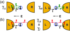
Figure 3: (Color online) Spin dynamics under bias in $\gamma$. The numbers denote the sequence of coherent motion. A down spin moves into the mediating atom (blue circle) and performs an exchange [green 2 in (a)] in $\gamma_{{}_{LL,RR}}$ and a singlet hopping [red 2 in (b)] in $\gamma_{{}_{LR,j}}$. The second part of (b) vanishes because of the reverse motion.

The matrix ${\rm\bf M}^{r}$ in Eq. (7) consists of two $3\times 3$ blocks that share the central element representing the mediating atom and two $2\times 2$ blocks at the corners. The three off-diagonal elements of the $3\times 3$ block represent the degrees of singlet coupling $\gamma_{{}_{LL(RR)}}$, e.g.,

$$\gamma_{{}_{LL}} = \frac{\langle\sum_{k}i(V_{km}^{*}c_{k\uparrow}^{L}+V_{km}^{*}c_{k\uparrow}^{R})c^{\dagger}_{m\uparrow}[j^{-L}_{m\downarrow},j^{+L}_{m\downarrow}]\rangle}{[\langle(\delta j^{-L}_{m\downarrow})^{2}\rangle\langle(\delta j^{+L}_{m\downarrow})^{2}\rangle]^{-1/2}},$$

and the incoherent double occupancy parameters

$$U_{j^{\pm}}^{L,R}=\frac{U}{2}[\langle D^{\pm L,R}_{m\uparrow\downarrow}\rangle+i(1-2\langle n_{m\downarrow}\rangle)]\frac{\langle j^{\pm L,R}_{m\downarrow}\rangle}{\langle(\delta j^{\pm L,R}_{m\downarrow})^{2}\rangle^{1/2}},$$

where $\langle D^{\pm L,R}_{m\uparrow\downarrow}\rangle=\langle[n_{m\downarrow},j^{\pm L,R}_{m\downarrow}](1-2n_{m\uparrow})\rangle/\langle j^{\pm L,R}_{m\downarrow}\rangle$. Hence, the real part ${\rm Re}[U_{j^{\pm}}^{L,R}]$ represents the probability of double occupancy by $j^{+}_{m\downarrow}$ or $j^{-}_{m\downarrow}$ coming from the left or right reservoir. In contrast, the elements of the $2\times 2$ corner blocks, i.e.,

$$\gamma_{{}_{LR}}=\frac{\langle\sum_{k}i(V_{km}^{*}c_{k\uparrow}^{L}+V_{km}^{*}c_{k\uparrow}^{R})c^{\dagger}_{m\uparrow}[j^{-L}_{m\downarrow},j^{+R}_{m\downarrow}]\rangle}{[\langle(\delta j^{-L}_{m\downarrow})^{2}\rangle\langle(\delta j^{+R}_{m\downarrow})^{2}\rangle]^{-1/2}},$$

and $\gamma_{{}_{j^{\mp}}}=\gamma_{{}_{j}}$, where

$$\gamma_{{}_{j^{\mp}}}=\frac{\langle\sum_{k}i(V_{km}^{*}c_{k\uparrow}^{L}+V_{km}^{*}c_{k\uparrow}^{R})c^{\dagger}_{m\uparrow}[j^{\mp L}_{m\downarrow},j^{\mp R}_{m\downarrow}]\rangle}{[\langle(\delta j^{\mp L}_{m\downarrow})^{2}\rangle\langle(\delta j^{\mp R}_{m\downarrow})^{2}\rangle]^{-1/2}}$$

describe the transition between two reservoirs. In Fig. 3, we present graphical illustrations of the third order hybridization processes embedded in $\gamma$ under bias. Singlet partner change and singlet hopping will occur to perform the process of Fig. 2 (a). In contrast, only singlet hopping is needed for Fig. 2 (b). The basis vectors in groups III and IV cause incoherent or backward motion that must be excluded in describing the unidirectional coherent motion at steady-state nonequilibrium. Therefore, neglecting groups III and IV is legitimate. The unidirectional movement of the Kondo singlet discussed in Fig. 2 guarantees $\gamma_{{}_{LR}}=\gamma_{{}_{j}}$ in Fig. 3 (b). This equality is considered as a condition of steady-state nonequilibrium.

The $5\times 5$ matrix of Eq. (7) gives three coherent and two incoherent poles in the LDOS. One of three coherent poles is located at the Fermi level and the other two are at $\pm\hbar\omega_{rt\ell}$, which are the levels represented by the dashed lines in Fig. 2 (b). The subscript $rt\ell$ indicates the resonant tunneling level. Hence, the tunneling current rapidly increases when the bias voltage reaches $\pm\hbar\omega_{rt\ell}$. A simple atomic limit analysis using the same ${\rm Re}[U^{L,R}_{j^{\pm}}]$ gives $\hbar\omega_{rt\ell}=\pm[(\gamma_{{}_{LL}}^{2}+\gamma_{{}_{RR}}^{2})/2]^{1/2}+O(U^{-2})$ and the spectral weight of the zero-bias peak as $Z_{F}=\gamma_{{}_{LL}}^{2}\gamma_{{}_{RR}}^{2}/2{\rm Re}[U^{L,R}_{j^{\pm}}]^{2}(\gamma_{{}_{LL}}^{2}+\gamma_{{}_{RR}}^{2})+O(U^{-2})$. The latter expression shows that the zero-bias peak is suppressed when $\gamma_{{}_{LL}}$ and $\gamma_{{}_{RR}}$ are imbalanced.

We show in the following that ${\rm Re}[U^{L,R}_{j^{+}}]>{\rm Re}[U^{L,R}_{j^{-}}]$ is introduced for symmetric reservoirs, which means that operator $j_{m\downarrow}^{+}$ induces more double occupancy than $j_{m\downarrow}^{-}$. For asymmetric reservoirs such as substrate ($L$) and tip ($R$) in scanning tunneling spectroscopy (STS), we use ${\rm Re}[U^{L}_{j^{+}}]>{\rm Re}[U^{L,R}_{j^{-}}]>{\rm Re}[U^{R}_{j^{+}}]$ to reflect different properties of reservoirs. In contrast, we adopt ${\rm Re}[U^{L}_{j^{-}}]={\rm Re}[U^{R}_{j^{-}}]$ because of the steady-state property of the current operator $j_{m\downarrow}^{-}$.

Before obtaining the $dI/dV$ line shapes, we first determine the coefficients $\beta_{mn}$. ${\rm Re}[\beta_{25}]$, for example, is given by ${\rm Re}[\beta_{25}]=\{\langle j^{-L}_{m\downarrow}(1-2n_{m\uparrow})\rangle\langle j^{+R}_{m\downarrow}(1-2n_{m\uparrow})\rangle+(1-2\langle n_{m\downarrow}\rangle)^{2}\langle j^{+L}_{m\downarrow}\rangle\langle j^{-R}_{m\downarrow}\rangle\}/4\langle(\delta n_{m\downarrow})^{2}\rangle\sqrt{\langle(\delta j^{+L}_{m\downarrow})^{2}\rangle}\sqrt{\langle(\delta j^{-R}_{m\downarrow})^{2}\rangle}$. The operators in the first term describe the self-energy dynamics that avoids double occupancy hong11 . We assume the same contribution of self-energy dynamics to all ${\rm Re}[\beta_{mn}]$ and the same relative fluctuations. Therefore, the differences among ${\rm Re}[\beta_{mn}]$ are attributable to the different signs for the current, i.e., $\langle j^{-L}_{m\downarrow}\rangle=-\langle j^{-R}_{m\downarrow}\rangle<0$. From the property $\langle j^{+L,R}_{m\downarrow}\rangle>0$, symmetric ${\rm Re}[\beta_{mn}]$ have the following mutual relations: ${\rm Re}[\beta_{12}]={\rm Re}[\beta_{14}]={\rm Re}[\beta_{15}]<{\rm Re}[\beta_{11}]={\rm Re}[\beta_{22}]={\rm Re}[\beta_{44}]={\rm Re}[\beta_{55}]={\rm Re}[\beta_{24}]={\rm Re}[\beta_{25}]={\rm Re}[\beta_{45}]$ and ${\rm Re}[\beta_{33}]=1$. In this study, we choose ${\rm Re}[\beta_{11}]=0.255$ and ${\rm Re}[\beta_{14}]=0.245$ based on the standard value ${\rm Re}[\beta_{mn}]=0.25$ that is obtained at the atomic limit hong11 . The same relative fluctuations give vanishing ${\rm Im}\beta_{mn}$ because they are given by the difference in the relative fluctuations.

The experimental $dI/dV$ line shapes under consideration are those of a quantum point contact with the closest side peaks given in Fig. 1 (b) of Ref. sarkozy and the STS for a Co atom placed on a Cu₂N layer on a Cu (100) substrate of Ref. otte . For the former, we employ the scenario of spontaneous formation of a localized spin at the bound state rejec ; ihna . Therefore, the Hamiltonian of Eq. (1) is applicable to both cases. The gate voltage dependence in the former system will be described in a future study. The theoretical $dI/dV$ line shapes given in Fig. 4 are obtained by using the matrix elements given in Table I. We set the energy unit to $\Delta\approx$ 1.5 and 5 meV for Figs. 4 (a) and 4 (b), respectively. The fittings are remarkably good.

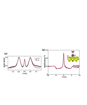
Figure 4: (Color online) Comparison of the theoretical line shape (red) using $\Delta\approx 1.5$ meV (a) and $\Delta\approx 5$ meV (b) with the experimental data (black) of the closest side peaks reported in Ref. sarkozy and the STS line shape of Ref. otte , respectively. We choose $\widetilde{\Gamma}/\Delta=0.82$ in (a) and an arbitrary unit for the theoretical $dI/dV$ in (b). Inset is STS setup otte ; choi .

Table I: Matrix elements for Fig. 4

	$\gamma_{{}_{LL}}$	$\gamma_{{}_{RR}}$	$\gamma_{{}_{j,LR}}$	${\rm Re}U^{L,R}_{j^{-}}$	${\rm Re}U_{j^{+}}^{L}$	${\rm Re}U_{j^{+}}^{R}$	${\rm Im}U_{j^{\pm}}^{L,R}$
(a)	0.38	0.38	0.5	0.98	1.1	1.1	0
(b)	0.86	0.76	0.43	2.8	7.0	1.62	0

As listed in Table I, we adopt a symmetric Kondo coupling ($\gamma_{{}_{LL}}=\gamma_{{}_{RR}}$) and ${\rm Re}[U_{j^{+}}^{L}]={\rm Re}[U_{j^{+}}^{R}]>{\rm Re}[U_{j^{-}}^{L,R}]$ in Fig. 4 (a) and an asymmetric Kondo coupling ($\gamma_{{}_{LL}}\neq\gamma_{{}_{RR}}$) and ${\rm Re}[U_{j^{+}}^{L}]>{\rm Re}[U_{j^{-}}^{L,R}]>{\rm Re}[U_{j^{+}}^{R}]$ in Fig. 4 (b). The zero-bias peak in Fig. 4 (a) is slightly suppressed by different contributions to double occupancy by operators $j^{+}$ and $j^{-}$ and the position of the side peak matches $\hbar\omega_{rt\ell}$ pretty well. The deviation outside the side peaks indicates that the range of bias independence of the LDOS covers the two side peaks. It is noteworthy that the line shape of Fig. 4 (b) shows a dip at zero bias when the insulating layer is removed mano . This implies that a strong Kondo coupling is established by inserting the insulating layer. Choi et al. choi , who studied the same system, observed that the meaningful structure of the line shape disappears when a Co atom is placed on top of a N atom. This indicates that the N atoms surrounding a Cu atom in a Cu₂N layer play the role of barrier that suppresses fluctuations and enhance ${\rm Re}[U_{j^{+}}^{L}]$ and the axial Kondo coupling connecting tip, Co atom, and Cu substrate. The large values of $\gamma_{{}_{LL}}$ and $\gamma_{{}_{RR}}$ given in Table I verify this fact. Choi et al. choi also show that the shoulder in Fig. 4 (b) is a variation of a coherent side peak.

In conclusion, our theoretical study clarifies that there are two different transport channels (Fig. 2). One uses the entangled Kondo singlet that connects the Kondo clouds in both reservoirs. Transport by the entangled Kondo singlet forms the zero-bias peak. The other uses resonant tunneling of a nonentangled Kondo singlet through the coherent tunneling level. This tunneling mechanism forms the side peak. Comparisons of the theoretical $dI/dV$ line shapes with those of the experimental ones (Fig. 4) clearly demonstrate the existence of the two transport channels.

The author thanks P. Coleman for suggesting the entangled singlet and A. Millis, N. Andrei, J. E. Han, E. Yuzbashyan, P. Kim, S.-W. Cheong, and P. Fulde for valuable discussions. This research was supported by the Basic Science Research Program through the NRF, Korea (2012R1A1A2005220), and was partially supported by a KIAS grant funded by MEST.

References

(1) N. S. Wingreen and Y. Meir, Phys. Rev. B 49, 11040 (1994).
(2) T. Fujii and K. Ueda, Phys. Rev. B 68, 155310 (2003).
(3) J. E. Han and R. J. Heary, Phys. Rev. Lett. 99, 236808 (2007).
(4) F. B. Anders, Phys. Rev. Lett. 101, 066804 (2008).
(5) H. R. Krishna-murthy, J. W. Wilkins, and K. G. Wilson,
Phys. Rev. B 21, 1003 and 1044 (1980).
(6) S. Sarkozy et al., Phys. Rev. B 79, 161307(R) (2009).
(7) A. F. Otte et al. Nat. Phys. 4, 847 (2008).
(8) J. Hong, Phys. J. Phys. Condens. Matter 23, 275602 (2011).
(9) H. Haug and A.-P. Jauho, Quantum Kinetics in Transport and Optics of
Semiconductors (Springer-Verlag, Berlin, 1996) Chap. 12.
(10) Y. Meir and N. S. Wingreen, Phys. Rev. Lett. 68, 2512
(1992).
(11) S. Hershfield, J. H. Davies, and J. W. Wilkins, Phys. Rev. B 46, 7046
(1992).
(12) V. Madhavan, W. Chen, T. Jamneala, M. F. Crommie, and N. S. Wingreen, Phys. Rev. B 64, 165412 (2001).
(13) A. Schiller and S. Hershfield, Phys. Rev. B 61, 9036(2000).
(14) M. Plihal and J. W. Gadzuk, Phys. Rev. B 63,
085404 (2001).
(15) J. Hong, J. Phys.: Condens. Matter 23, 225601 (2011).
(16) P. O. Löwdin, J. Math. Phys. 3, 969 (1962).
(17) H. C. Manoharan, C. P. Lutz, and D. M. Eigler, Nature
403, 512 (2000).
(18) T. Choi, C. D. Ruggiero, and J. A. Gupta, J. Vac. Sci. Technol.
B 27, 887 (2009).
(19) T. Rejec and Y. Meir, Nature 442, 900
(2006).
(20) S. Ihnatsenka and I. V. Zozoulenko,
Phys. Rev. B 76, 045338 (2007).