COMPUTING INTRINSIC LYMAN-ALPHA FLUXES OF F5 V TO M5 V STARS

Abstract

The Lyman-$\alpha$ emission line dominates the far-ultraviolet spectra of late-type stars and is a major source for photodissociation of important molecules including H₂O, CH₄, and CO₂ in exoplanet atmospheres. The incident flux in this line illuminating an exoplanet’s atmosphere cannot be measured directly as neutral hydrogen in the interstellar medium (ISM) attenuates most of the flux reaching the Earth. Reconstruction of the intrinsic Lyman-$\alpha$ line has been accomplished for a limited number of nearby stars, but is not feasible for distant or faint host stars. We identify correlations connecting the intrinsic Lyman-$\alpha$ flux with the flux in other emission lines formed in the stellar chromosphere, and find that these correlations depend only gradually on the flux in the other lines. These correlations, which are based on HST spectra, reconstructed Lyman-$\alpha$ line fluxes, and irradiance spectra of the quiet and active Sun, are required for photochemical models of exoplanet atmospheres when intrinsic Lyman-$\alpha$ fluxes are not available. We find a tight correlation of the intrinsic Lyman-$\alpha$ flux with stellar X-ray flux for F5 V to K5 V stars, but much larger dispersion for M stars. We also show that knowledge of the stellar effective temperature and rotation rate can provide reasonably accurate estimates of the Lyman-$\alpha$ flux for G and K stars, and less accurate estimates for cooler stars.

1 INTRODUCTION

The discovery of large numbers of extrasolar planets (exoplanets) has stimulated many observational and theoretical studies of their atmospheric chemical compositions. In particular, the habitability of an exoplanet at a given distance from its host star is generally thought to depend on the total flux received from the host star, the availability of greenhouse gasses, and the presence of biomarkers such as O₂ and O₃ (but see Feng et al. (2012)). Estimates of the chemical composition of exoplanet atmospheres depend crucially on the near-ultraviolet (NUV, $\lambda=$1700-3200 Å), far-ultraviolet (FUV, $\lambda$ = 1170–1700 Å), extreme ultraviolet (EUV, $\lambda=$300–911 Å), XUV ($\lambda=$100-300 Å), and X-ray ($\lambda<100$ Å) radiation from the host star, which control important molecular photodissociation and photoionization processes.

Early interest concerning the influence of a star on its substellar companions was focused on the erosion of volatile gasses from the primordial atmospheres of the terrestrial planets of our Solar System (especially Mars and Venus) by dissociative recombination powered by solar ultraviolet radiation and pickup-ion stripping by the solar wind. These processes would have been enormously enhanced when the Sun was young and more magnetically active than today (e.g., Zahnle & Walker, 1982). Using a data base of solar-type stars in young clusters of known age and extrapolating from solar fluxes over the sunspot cycle, Ayres (1997) showed that photoionization rates relevant to the Martian situation scale as power laws in time (as anticipated in the earlier Zahnle & Walker paper). Furthermore, the UV flux behavior could be reliably traced back to the epoch of the Late Heavy Bombardment (at solar age $\sim$800 Myr), because by then rotation rates of young G stars had funneled into a narrow distribution from an initially more diverse behavior (Delorme et al., 2011). It is the stellar spin that largely governs the degree of magnetic activity, and the decay of that spin by wind braking that causes the rapid decline of the UV and X-ray activity with increasing age.

More recently, the “Sun in Time” project (Ribas et al., 2005, 2010) and Sanz-Forcada et al. (2011) have extended the earlier work to a wider range of high energy measurements, especially including the important 912–1170 Å Far Ultraviolet Spectroscopic Explorer (FUSE) band, and to a broader range of spectral types (G0 to G5), utilizing field stars whose ages must be inferred indirectly, but are more accessible to observation than the mostly distant cluster members. These studies also showed that in different wavelength bands, power laws could be used to describe the decay of chromospheric and coronal radiation over time.

Ribas et al. (2005) called attention to the importance of the H I Lyman-$\alpha$ line (1215.67 Å), which is by far the brightest FUV emission line. They showed that for the Sun, the Lyman-$\alpha$ line flux is about 20% of the total flux between 1 and 1700 Å. The relative importance of the Lyman-$\alpha$ line is even more important for cooler stars as the photospheric emission at $\lambda>1700$ Å decreases rapidly with decreasing effective temperature.

Since important molecules in planetary atmospheres, including H₂O, CO₂, and CH₄, have photodissociation cross sections that peak below 1700 Å, Lyman-$\alpha$ radiation can be the dominant cause of photodissociation for these and other molecules. For example, the solar Lyman-$\alpha$ line is responsible for 51% of the photodissociation rate of H₂O by solar UV radiation between 1148 and 1940 Å, and 71% of the total photodissociation rate of CH₄ by solar radiation between 56 and 1520 Å. However, recent models of exoplanet atmospheres that include photoionization, e.g., models for WASP-12b (Kopparapu, Kasting, & Zahnle, 2012), typically do not include realistic values for the stellar Lyman-$\alpha$ flux. In this recent model, the FUV fluxes were obtained from the compilation of Pickles (1998) that is based on International Ultraviolet Explorer (IUE) spectra without a large correction for interstellar absorption in the Lyman-$\alpha$ line or geocoronal Lyman-$\alpha$ emission. New ultraviolet spectra of six M dwarf host stars observed with spectrographs on the Hubble Space Telescope by France et al. (2012b) provide an observational basis for more realistic photochemical models of exoplanet atmospheres.

While exoplanet atmospheres absorb the Lyman-$\alpha$ flux from their host stars without attenuation, neutral hydrogen in the interstellar medium scatters most of the Lyman-$\alpha$ flux out of the line-of-sight between the star and Earth. One must therefore correct for interstellar absorption by reconstructing the stellar Lyman-$\alpha$ profile and flux. For pre-main sequence stars with disks, Herczeg et al. (2004) and Schindhelm et al. (2012) showed that the fluorescent H₂ emission lines pumped by Lyman-$\alpha$ provide a useful diagnostic for reconstructing the intrinsic Lyman-$\alpha$ emission line. For 62 main-sequence and giant stars without H₂ fluorescence, Wood et al. (2005) reconstructed Lyman-$\alpha$ fluxes using interstellar H I column densities and velocities inferred from the deuterium Lyman-$\alpha$ and metal lines. France et al. (2012a) developed an alternative reconstruction technique in which the widths and strengths of one or two Gaussian emission lines representing Lyman-$\alpha$ and the velocities and column densities of interstellar absorption features are iteratively varied to obtain a solution that best fits the observed Lyman-$\alpha$ line wings. Both techniques require high-resolution spectra with good signal/noise and minimal contamination by geocorona Lyman-$\alpha$ emission. The only available spectrograph that can obtain such data is the Space Telescope Imaging Spectrograph (STIS) on HST. High instrumental sensitivity, especially important for faint M dwarfs, increasing interstellar hydrogen column densities with distance, and difficult-to-obtain HST observing time limit the number of stars for which Lyman-$\alpha$ fluxes can be reconstructed by these two techniques.

The objective of this study is to find different methods for infering the Lyman-$\alpha$ flux incident on the atmospheres of exoplanets for stars when high-resolution Lyman-$\alpha$ spectra are not available. These methods should be applicable to a broad range of stars including M dwarfs, which are very numerous and could support habitable planets with short orbital periods. One proposed method is to use correlations of reconstructed Lyman-$\alpha$ line fluxes with other stellar features (lines of O I and C II) formed in the same temperature range as Lyman-$\alpha$, lines of Mg II and Ca II formed at slightly lower temperatures, and lines of C IV formed at somewhat higher temperatures. Our hypothesis is that ratios of the Lyman-$\alpha$ line flux to fluxes in these other lines should be similar for stars in limited ranges of spectral type with only a small dependence on stellar activity as indicated by the emission line fluxes. Empirical support for this hypothesis comes from the similar power law slopes of UV emission lines (Ayres, 1997; Ribas et al., 2005) and the correlation of Lyman-$\alpha$ and Mg II fluxes (Wood et al., 2005). The similar shapes of the chromosphere and transition region thermal structures for regions on the Sun with very different heating rates (Fontenla et al., 2011) provides theoretical support for our hypothesis.

The paper is structured as follows. In section 2 we describe our selection of targets that have reconstructed Lyman-$\alpha$ and other UV emission line fluxes. Section 3 describes our procedure for reconstructing the intrinsic Lyman-$\alpha$ flux using correlations with other UV emission lines and the errors and uncertainties of this method. Section 4 describes an extension of this procedure using correlations with ground-based Ca II H and K line fluxes, and section 5 describes how correlations with X-ray fluxes can be used to predict the intrinsic Lyman-$\alpha$ flux. Section 6 describes how the stellar effective temperature and rotation rate can provide rough estimates of the intrinsic Lyman-$\alpha$ flux when no emission line fluxes are available. The final section lists our conclusions. In a subsequent paper, we will apply the flux correlation technique to estimating stellar EUV radiation, which is responsible for photoionizing hydrogen and other species, heating outer atmospheres, and driving mass loss from exoplanets.

2 TARGET SELECTION

Our target list consists of all F5 to M5 main sequence stars for which reconstructed Lyman-$\alpha$ fluxes are now available. Wood et al. (2005) reconstructed Lyman-$\alpha$ line profiles observed by STIS in its medium (spectral resolution $\approx\lambda/45,000$) and high-resolution ($\approx\lambda/100,000$) echelle modes using interstellar deuterium Lyman-$\alpha$ and metal absorption lines to model the interstellar H I column density as a function of wavelength across the hydrogen Lyman-$\alpha$ line. They provided reconstructed Lyman-$\alpha$ line fluxes for 40 main-sequence stars with spectral types F5 to M5, together with Mg II h and k line and X-ray fluxes for most of these stars. We also include five M dwarf stars that are known to host exoplanets. The Lyman-$\alpha$ fluxes for these stars were reconstructed from STIS grating and echelle spectra using an iterative technique to measure the intrinsic Lyman-$\alpha$ profile and the interstellar absorption (France et al., 2012a).

For most these stars, we have measured fluxes of the H I 1215.67 Å, O I 1304.86 Å + 1306.03 Å, C II 1335.71 Å, and C IV 1548.19 Å + 1550.77 Å lines. In the semi-empirical solar chromosphere and transition region model computed by Avrett & Loeser (2008), the peak contributions to the line center emission for these lines are at temperatures near 40,000 K, 6,700 K, 29,500 K, and 68,000 K, respectively. However, the wings of these lines are formed over a range of cooler temperatures. We did not use fluxes of the O I 1302.17 Å and C II 1334.53 Å lines as these lines show strong interstellar absorption. We extracted the O I, C II and C IV line fluxes from Cosmic Origin Spectrograph (COS) (Green et al., 2012) data with spectral resolution ($\approx\lambda/17,000$) available through the Mikulski Archive for Space Telescopes (MAST) and the well-calibrated STIS spectra from the StarCAT (Ayres, 2010) website. In a few cases we used data obtained with the Goddard High Resolution Spectrograph (GHRS) instrument on HST. The O I data obtained with COS are not usable because of airglow contamination. We subtracted the underlying continuum from the emission line fluxes. Line fluxes for the solar-mass stars were measured by Linsky et al. (2012).

We also include solar spectral irradiance data observed with the Solar Radiation and Climate Experiment (SORCE) on the Solar-Stellar Irradiance Comparison Experiment II (SOLSTICE II) (Woods et al., 2009; Snow et al., 2005). These are integrated sunlight spectra directly comparable with the stellar data. The 2008 April 10–16 data refer to the very quiet Sun, and the 2003 October 27 and November 10 data refer to the Sun when it was very active.

Table 1 summarizes the stellar and emission line fluxes f(line) in ergs cm^-2 s^-1 at a distance of 1 AU for 45 stars, the quiet Sun, and the active Sun at two different times. Since most of the stars are variable, especially in the FUV, the fluxes refer to a single time and are not time averages. For most of the stars the STIS Lyman-$\alpha$ spectra and the COS spectra of the O I, C II, and C IV were obtained at different times. Since stellar UV radiation varies with time especially for M dwarfs and active warmer stars, ratios of the Lyman-$\alpha$ flux to other emission lines will have systematic errors compared to the stars for which all of the emission lines were observed at nearly the same time.

3 CORRELATIONS OF RECONSTRUCTED LYMAN-$\alpha$ FLUX WITH EMISSION LINES FORMED IN THE CHROMOSPHERE AND TRANSITION REGION

3.1 F5 V to G9 V stars

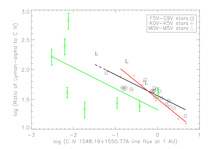
Figure 1: Plot of the ratio of the Lyman-$\alpha$ to C IV 1548+1550 Å line flux vs. the C IV line flux at 1 AU. Included are stars between spectral types F5 V and M5 V, divided into three spectral type bins, the quiet Sun and the active Sun at two different times. The solar data are indicated by Sun symbols, and the L symbol refers to a star with low metal abundance [Fe/H] $<-0.30$. The solid lines are least-squares fits for each spectral type bin excluding the L stars and the Sun. The ratio for $\alpha$ Cen A is closest to the solar ratios. The errors bars are 20% for stars using the Wood et al. (2005) correction for missing Lyman-$\alpha$ flux or 30% for stars using the France et al. (2012a) correction for missing Lyman-$\alpha$ flux.

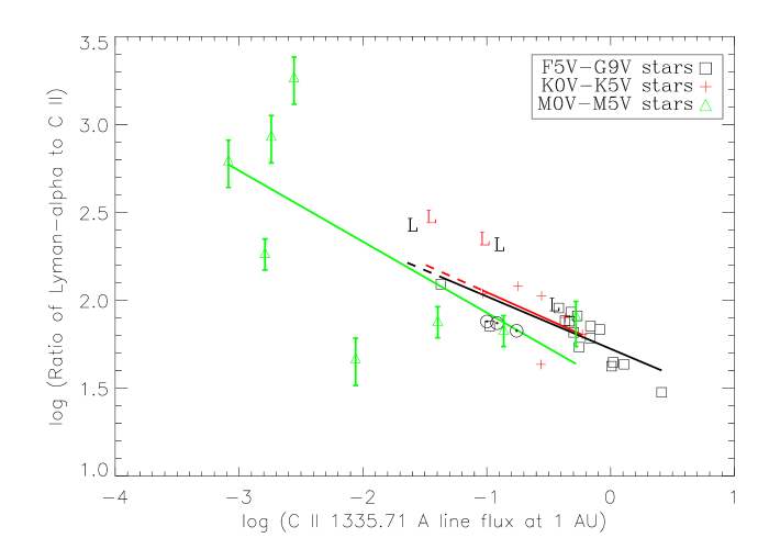
Figure 2: Same as Figure 1 except for the Lyman-$\alpha$ to C II 1335 Å line flux ratio vs. the C II line flux at 1 AU.

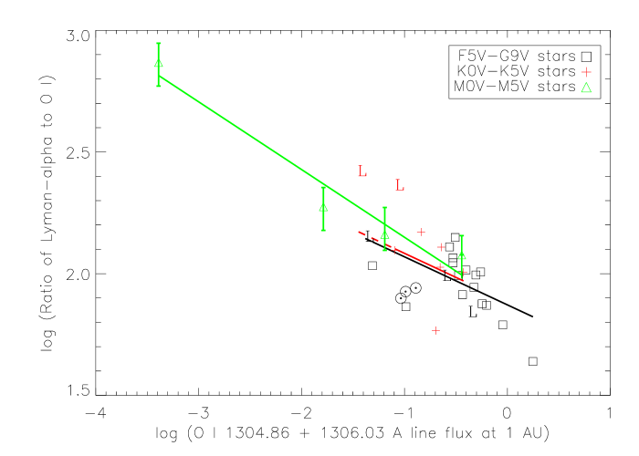
Figure 3: Same as Figure 1 except for the Lyman-$\alpha$ to O I 1304.86 + 1336.03 Å line flux ratio vs. the O I line flux at 1 AU. The small dispersion of the line flux ratios for the M stars may be unrepresentative given the small number of data points.

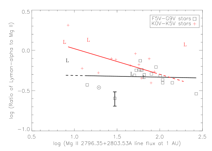
Figure 4: Same as Figure 1 except for the Lyman-$\alpha$ to Mg II 2796 + 2803 Å line flux ratio vs. the Mg II line flux at 1 AU.

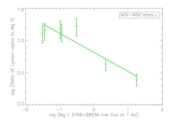
Figure 5: Plot of the Lyman-$\alpha$ to Mg II 2796 + 2803 Å line flux ratio vs. the Mg II line flux at 1 AU for the M0 to M5 stars. The solid line is the least-squares fit to the data. The errors bars are 20% for stars using the Wood et al. (2005) correction for the missing Lyman-$\alpha$ flux or 30% for stars using the France et al. (2012a) correction for the missing Lyman-$\alpha$ flux.

Table 1 lists the measured fluxes for 21 F5–G9 stars and the Sun at three different times and activity levels. We plot in Figure 1 the flux ratio R(C IV) = f(Lyman-$\alpha$)/f(C IV) vs. f(C IV) with line fluxes measured in ergs cm^-2 s^-1 at a distance of 1 AU. Figures 2–5 show similar plots of R(line) = f(Lyman-$\alpha$)/f(line) vs. f(line) using the previously described C II, O I, and Mg II lines. The R(line) ratios for the F5–G9 stars in Figures 1–4 follow tight trajectories of decreasing R(line) with increasing f(line). In Table 1 we list the iron abundances relative to hydrogen [Fe/H] listed in the SIMBAD data base. Three of the F5–G9 stars (HR 4657, $\chi$ Her, and $\tau$ Cet) have large iron depletions (defined as [Fe/H] $<0.3$), and often have higher R(line) values than other stars with similar fluxes and [Fe/H] values close to the solar. This behavior is expected since R(line) should increase as the line’s metal abundance decreases, but whether or not R(line) is inversely proportional to [Fe/H] will be considered in the next section. We therefore exclude the low [Fe/H] stars when computing least-squares fits for the remaining F5–G9 stars. The coefficients for these fits, log[R(line)] = A + Blog[f(line)], are listed in Table 2. We note that the least-squares fits, which do not include the solar data, are close to the solar data. Also, the $\alpha$ Cen A ratios are similar to the quiet and active Sun ratios even though the solar and stellar data are measured by different instruments. Table 2 shows that the mean dispersions of the F5–G9 stars about the best fit lines are 18–24%.

3.2 K0 V to K5 V stars

There are a total of 16 stars in this group: 15 have Mg II fluxes, and 8 have C IV, C II fluxes and O I fluxes. The least-squares fits to the R(line) ratios for the K0 V – K5 V stars have similar slopes to the fits to the R(line) ratios for the F5–G9 stars and similar dispersions (15–30%) about the fit lines. The K0 V-K5 V stars have a wide range in rotational periods (0.38 days for Speedy Mic to 43 days for $\alpha$ Cen B), but there is no strong trend of R(line) with rotational period and thus with activity. Eight of these stars are classified in SIMBAD as either BY Dra type varables or RS CVn type variables, but we can find no information on the companion stars which are likely fainter and cooler than the primary stars.

3.3 M0 V to M5 V stars

We analyze spectra of nine M0 V to M5.5 V stars with reconstructed Lyman-$\alpha$ fluxes. Five of these are exoplanet host stars. We plot R(line) vs. log[f(line)] in Figures 1–3 and 5. The dispersion of the data about the fit lines is much larger for the M stars than for the F5–K5 stars primarily due to their much larger time variability as described in the following section. The dispersion in R(O I) for the M stars, however, may be unrepresentative given the small number of data points.

3.4 Errors and Uncertainties

In this analysis, we identify four causes of uncertainty in the R(line) values: flux measurement errors, Lyman-$\alpha$ line reconstruction errors, uncertain atomic abundances, and unknown time variability. We can estimate the error magnitudes or at least identify the first three types of errors, but time variability errors cannot be measured with the existing data and are therefore systematic.

The smallest errors are typically flux-measurement errors for the C IV, C II, O I, and Mg II lines. These are typically less than 2% for the STIS data in StarCAT and the COS data sets, but can be as large as 5–20% for the faintest M dwarfs. Uncertainties in the reconstruction of the Lyman-$\alpha$ lines are usually larger than the line flux measurement errors. Wood et al. (2005) estimated 20% for typical errors in reconstructing Lyman-$\alpha$ line fluxes. In order to compare the two reconstruction methods, we re-fit the observed Lyman-$\alpha$ line profiles of several stars in the Wood et al. (2005) sample with the iterative least-squares technique (France et al., 2012a). For the favorable case of AU Mic, a star with high signal/noise data and a single ISM absorption feature, the agreement in the reconstructed fluxes between the two techniques is within 5%. For the unfavorable case of AD Leo, a star with several ISM velocity components along the line of sight, the disagreement is about 30%. In Figures 1-5, we plot representative errors of 20% for the R(line) ratios based on the Wood et al. (2005) reconstruction, or 30% for the faint M dwarfs based on the France et al. (2012a) reconstruction. As shown Table 2, the mean dispersions of the F5–G9 and K0–K5 stars (ignoring the low metal abundance stars) are in the range 18–30%, which is consistent with our estimates of the Lyman-$\alpha$ reconstruction errors and smaller time variability errors.

We have excluded stars with low iron abundances ([Fe/H]$<0.3$) from the sample of stars used to make the least-squares fits. The [Fe/H] abundances for the F, G, and K stars were obtained from the SIMBAD data base. Accurate abundance measurements for M dwarfs require special techniques given the complexity of their spectra. Recent work includes calibration of the offset of stars in the H-R diagram relative to the main sequence (Johnson & Apps, 2009) and measurements of Na I and Ca I absorption lines in near-IR spectra (Rojas-Ayala et al., 2010). Rojas-Ayala et al. (2012) have revised their earlier work and compared their new results to earlier studies. We therefore adopt their [Fe/H] measurements for AD Leo, EV Lac, and the exoplanet host stars GJ 876, GJ 581, and GJ 436. We adopt the [Fe/H] value for GJ 832 measured by (Rojas-Ayala et al., 2010). Cayrel de Strobel et al. (2001) lists [Fe/H]=–0.54 for GJ 667C, but we do not expect this star to have a significant underabundance as the other host stars show normal or superrich abundances. The young star AU Mic should have near solar abundances, and Proxima Cen should have the near-solar abundances of $\alpha$ Cen A and B.

For each low iron abundance star, Table 4 lists the value of [Fe/H], and for each spectral line the log of the difference, which we refer to as “delta”, between R(line) and the least-squares fit line at the value of f(line). If the deltas were only due to low metal abundance and the abundances of carbon, oxygen, and magnesium relative to the Sun were the same as for iron, then the observed deltas should be the negative of the log iron depletions. This is not the case, but the data in Table 4 show some interesting trends. For example, the deltas seen in the C IV and C II lines (and to some extent in the O I line) are nearly the same for each star, implying that the abundances of carbon and oxygen may be important factors in determining the deltas. However, the deltas are much smaller than –[Fe/H] for the F5–G9 and K0–K5 stars. Thus metal depletion cannot be the only factor determining the deltas, and the thermal structures of the atmospheres of stars of different spectral type likely play a role. Since the many lines of Fe, Mg, and Ca are the main cooling agents of the lower solar chromosphere (Anderson & Athay, 1989), lower abundances of these elements will change the energy balance and thus the thermal structure.

Since the deltas for the Mg II lines of the F5–K5 stars are mostly smaller than those for the C IV, C II, and O I lines, there will likely be a smaller uncertainty when estimating R(Mg II) from the least-squares fits compared to using R(line) for the C IV, C II, and O I lines. However, it is important to correct for interstellar absorption in the Mg II lines, which requires high-resolution spectra. Since interstellar absorption is minimal for the C IV lines, the C II 1335 Å line, and the O I 1304 and 1306 Å lines, lower resolution spectra of these lines can be used without interstellar corrections for estimating R(line) and thus the intrinsic Lyman-$\alpha$ flux.

In most cases, the STIS spectra containing the Lyman-$\alpha$ line and the COS or STIS spectra used for extracting the other line fluxes were obtained at different times. For these stars the R(line) ratios will depend on time variations in the stellar UV emission. The importance of time variability for different types of stars can be estimated from the mean dispersion and RMS dispersions of the R(line) ratios about the least-squares fits. These dispersions for the M stars listed in Table 2 are much larger than for the F5–K5 stars and much larger than the 20–30% uncertainty associated with the Lyman-$\alpha$ reconstructions. This behavior is expected since M stars are more variable and flare more often than the warmer stars.

4 CORRELATION OF RECONSTRUCTED LYMAN-$\alpha$ FLUX WITH Ca II EMISSION

The hydrogen H$\alpha$ (6563 Å) and Ca II H and K (3933 and 3968 Å) lines formed in the chromosphere are observable by ground-based telescopes. However, the H$\alpha$ line is difficult to analyze since increasing heating first deepens the absorption line and then produces an emission feature. We consider instead the Ca II lines because the emission in the centers of the broad photospheric absorption lines is a good indicator of the chromospheric heating rate. An important difficulty is distinguishing the chromospheric emission inside of the H1 and K1 features that define the emission core from the photospheric emission that would be present in the absence of a chromosphere. For active stars and especially M dwarfs, this is not a large uncertainty as the photospheric emission is faint compared to the bright chromospheric emission. For the less active G stars, the photospheric emission is comparable to or larger than the chromospheric emission. It is therefore essential to correct for the photospheric emission as we wish to correlate chromospheric Ca II emission with the intrinsic Lyman-$\alpha$ flux.

Different authors has estimated the photospheric emission in and near the core of the Ca II lines in different ways. Using high-resolution spectra, Linsky et al. (1979) and Pasquini et al. (1988) measured the flux in the Ca II emission line cores between the H1 and K1 minima features and subtracted the small amount of flux in these wavelength intervals predicted by radiative equilibrium model photospheres. Robinson et al. (1990) and Browning et al. (2010) fitted the photospheric H and K absorption lines with Gaussians and then subtracted the flux interpolated in the line cores from the measured Ca II emission. This approach somewhat overcorrects for the photospheric emission, but the error is small for the very cool stars that they observed. The resulting chromospheric Ca II fluxes at 1 AU are listed in columns 6 and 7 of Table 3.

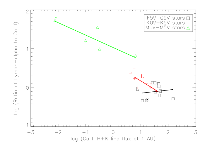
Figure 6: Plot of the Lyman-$\alpha$ to Ca II 3933 + 3968 Å line flux ratio vs. the Ca II line flux at 1 AU for the M0 to M5 stars. The solar data are indicated by the Sun symbol, and the L symbol refers to a star with low metal abundance [Fe/H] $<-0.30$. The solid lines are least-squares fits for each spectral type bin excluding the L stars and the Sun.

Other observers have measured the S index, which is the flux in 1.09 Å bandpasses centered on the H and K line emission cores divided by the flux in continuum windows. Hartmann et al. (1984) provided a correction for the photospheric flux within the bandpass but outside of the H1 and K1 features using high-resolution spectra of stars with weak H and K emission. Columns 8 and 9 of Table 3 show the time-averaged Ca II fluxes obtained at Mt. Wilson by Noyes et al. (1984) and Baliunas et al. (1995) after subtracting the photospheric flux following Hartmann et al. (1984). Columns 10 and 11 show Ca II fluxes obtained by Henry et al. (1996), Hall et al. (2007, 2009), and Lockwood et al. (2007) using a similar approach. The last column in Table 3 lists the fluxes of Southern hemisphere stars obtained by Cincunegui et al. (2007). We plot in Figure 6 the ratio of Lyman-$\alpha$ to Ca II flux, R(Ca II), using the average of the Ca II fluxes for all of the data in Table 3, except for the Cincunegui et al. (2007) fluxes which appear to be systematically smaller than the fluxes obtained from the other sources..

The R(Ca II) data in Figure 6 for each spectral type bin show relatively small scatter about the least-squares fit lines. We find that the dispersion (see Table 2) is smallest for the K stars (only 20.6%), and larger for the variable M stars. The dispersion of 42% for the G stars likely results from uncertainty in the photospheric flux correction which is large for G stars. Thus the Ca II H and K line flux can be used to estimate the intrinsic Lyman-$\alpha$ flux from the fit lines, provided one can remove the photospheric component from the observed line core fluxes.

5 CORRELATION OF RECONSTRUCTED LYMAN-$\alpha$ FLUX WITH X-RAY EMISSION

Except for the highly variable M dwarfs for which the Lyman-$\alpha$ and other emission lines were observed at different times, the correlations of reconstructed Lyman-$\alpha$ flux with emission lines formed at similar or somewhat higher temperatures in the chromosphere and transition region generally have small scatter about the least-squares fit lines. This behavior results from increasing mechanical heating shifting the chromospheric thermal structure to higher densities while keeping a similar shape (Fontenla et al., 2011). Thus all of the emission lines brighten together roughly proportional to density squared. Ayres (1997), Ribas et al. (2005), and others have noted that slopes of power-law relations between X-ray and chromosphere line flux are generally near 2.0 rather than a linear relation. Also, soft X-ray emission as measured, for example, by ROSAT is highly sensitive to coronal temperature and is more time variable than chromospheric emission. For these reasons, we did not anticipate a tight correlation between reconstructed Lyman-$\alpha$ flux and X-ray flux. Wood et al. (2005) plotted X-ray flux vs reconstructed Lyman-$\alpha$ flux for F–M dwarfs and giants showing correlations, but with large scatter for each type of star.

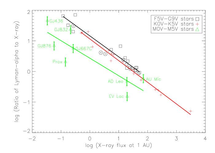
Figure 7: Plot of the ratio of Lyman-$\alpha$ to X-ray flux vs. the Lyman-$\alpha$ line flux at 1 AU for all stars in our sample with X-ray data. The solid lines are least-squares fits to the data for the F5 V–G9 V, K0 V–K5 V, and M0 V–M5 V stars. Data for the quiet Sun, moderately active Sun, and active Sun are indicated by the dotted circle symbols (from left to right respectively).M dwarfs stars are identified by name.

We plot in Figure 7 the R(X)=f(Lyman-$\alpha$)/f(X-ray) ratios vs. X-ray flux at 1 AU for the stars in Table 1 using the ROSAT PSPC X-ray fluxes cited by Wood et al. (2005) or more recent X-ray flux measurements using Chandra and XMM-Newton (see the references cited in the footnotes of Table 1). The X-ray flux for GJ 667C, which was obtained with the HRI instrument on ROSAT rather than the PSPC, is uncertain due to the close proximetry of GJ 667A and GJ 667B. Judge, Solomon, & Ayres (2003) estimated solar X-ray fluxes through the ROSAT PSPC bandpass from full disk solar observations by the SNOE-SXP instrument. For the quiet Sun, moderately active Sun, and active Sun, we use their X-ray luminosities, $\log L_{X}=$ 26.8, 27.75, and 27.9, respectively.

The Lyman-$\alpha$/X-ray flux data show correlations with small scatter for the F5–G9 and K0–K5 dwarfs. The quiet and active solar data are consistent with the least-squares fit for the other F5–G9 stars. The mean dispersions listed in Table 2 are 29.8% for the F5–G9 dwarfs and 22.2% for the K0–K5 dwarfs, which are similar to the mean dispersions for the C IV, C II, O I, Mg II, and Ca II lines. The mean dispersion for the M dwarfs is much larger than for the F5–K5 stars, although the slope of the fit line is similar to that of the warmer stars. X-ray time variability is the most likely cause of the large scatter of the M stars as the X-ray and Lyman-$\alpha$ data were obtained at different times. Despite the factor of 2–3 scatter about the M star fit line, the similar slope of the fit line to those for the warmer stars suggests that one can use the M dwarf fit line to estimate the Lyman-$\alpha$ flux of an M dwarf at the time of an X-ray measurement with an uncetainty much smaller than the dispersion shown in Table 2. We note that GJ832 is plotted very close to the quiet Sun in Figure 7, and that GJ832 (M1.5 V) and AU Mic (M0 V) are consistent with the fit lines for the K0–K5 stars. This suggests that the R(X) vs. X-ray flux correlation for K stars may also be useful for estimating the intrinsic Lyman-$\alpha$ flux of early M dwarfs.

6 CORRELATION OF THE RECONSTRUCTED LYMAN-$\alpha$ FLUX WITH STELLAR EFFECTIVE TEMPERATURE AND ROTATION

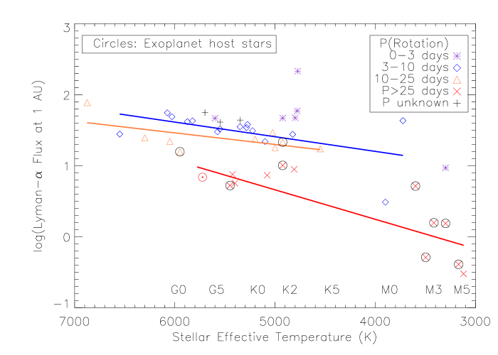
Figure 8: Lyman-$\alpha$ flux at 1 AU vs. stellar effective temperature. The stars are grouped according to stellar rotation period: ultrafast rotators ($P_{\rm rot}<3$ days), fast rotators (3–10 days), moderate rotators (10–25 days), and slow rotators ($>25$ days). Rotation period is a rough measure of the magnetic heating rate in the star’s chromosphere and corona. Host stars of exoplanets are circled and the quiet Sun is marked as a circled dot. Least-squares fit lines are shown for the fast, moderate, and slow rotators.

We now consider whether the stellar Lyman-$\alpha$ flux of main-sequence stars can be estimated simply from the stellar effective temperature ($T_{\rm eff}$). We plot in Figure 8 the Lyman-$\alpha$ flux for all of the stars in Table 1 vs. $T_{\rm eff}$. At each value of $T_{\rm eff}$, there is a dispersion in the Lyman-$\alpha$ flux that increases from a factor of 4 near $T_{\rm eff}=6000$ K to a factor of 1000 for the M stars. The range in Lyman-$\alpha$ flux at a given $T_{\rm eff}$ is reduced significantly by grouping the stars according to their rotation period ($P_{\rm rot}$), which is a rough measure of magnetic heating rates in the chromosphere and corona. We show least squares fits, log f(Lyman-$\alpha$) = A + BT_eff, for the stars in three groups: fast rotators ($P_{\rm rot}$ = 3–10 days), moderate rotators (10–25 days), and slow rotators ($>25$ days). The coefficients for these fits are listed in Table 5. Compared to the least-squares fits, the Lyman-$\alpha$ flux dispersion within each rotational period group is 32–85% and largest for the M stars. Therefore, estimates of the Lyman-$\alpha$ flux based only on a star’s $T_{\rm eff}$ and $P_{\rm rot}$ are reasonably accurate for G stars but not for the cooler stars.

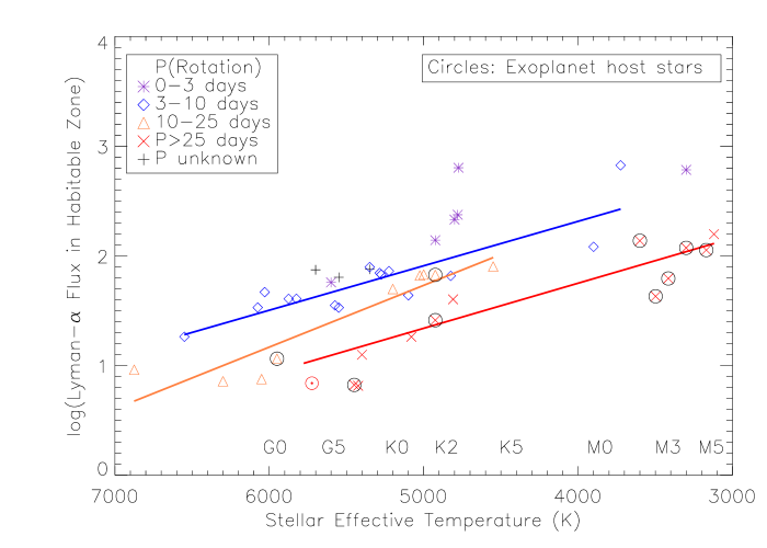
Figure 9: Same as Figure 8, except that the Lyman-$\alpha$ flux is evaluated in the habitable zone for an exoplanet.

In Figure 9, we plot the Lyman-$\alpha$ flux in the habitable zone (HZ) of an exoplanet, where the distance from the star to the habitable zone is estimated approximently as proportional to the stellar luminosity, $d_{\rm HZ}=(R_{\star}/R_{\odot})(T_{\star}/T_{\odot})^{2}$ AU. The location of the HZ, the region around a star where life forms are thought to be possible, involves many other considerations including greenhouse gases, orbital eccentricity and stability, and atmospheric chemical composition (Kasting & Catling, 2003). In this HZ plot, the dispersion of the Lyman-$\alpha$ flux is reduced somewhat for the M stars (see Table 5). Lyman-$\alpha$ fluxes in the HZ trend significantly higher with decreasing $T_{\rm eff}$, and the quiet Sun has nearly the smallest value of Lyman-$\alpha$ flux. Exoplanets of most of the stars discussed in this paper receive significantly larger Lyman-$\alpha$ fluxes and thus have higher molecular dissociation rates in their atmospheres. This is especially true for M dwarfs, which have smaller radii and lower effective temperatures than the Sun. Exoplanets in the HZs of the five M dwarfs in this study receive about 10 times the Lyman-$\alpha$ flux as the Earth receives from the quiet Sun. We therefore conclude that large FUV fluxes are received by exoplanets in their HZs from their M dwarf host stars contrary to some previous assumptions. Also, the Lyman-$\alpha$ fluxes for stars with exoplanets do not appear to differ from stars without discovered exoplanets in these two plots.

7 CONCLUSIONS

We have identified five methods for reconstructing or estimating the intrinsic Lyman-$\alpha$ stellar fluxes of main-sequence stars between spectral types F5 and M5. Whether a given method can be used and its accuracy depends on the quality of the available data. The first and most accurate method developed by Wood et al. (2005) requires high-resolution spectra of the Lyman-$\alpha$ line and knowledge of the interstellar velocity structure based on high-resolution spectra of the deuterium Lyman-$\alpha$ and metal lines. Wood et al. (2005) estimates typical errors of 20% in the reconstructed Lyman-$\alpha$ line fluxes using this method, but at present only the STIS instrument on HST can provide such data for nearby stars.

The second method developed by France et al. (2012a) also requires high-resolution spectra of the hydrogen Lyman-$\alpha$ line, but does not require spectra of the deuterium Lyman-$\alpha$ line or any other interstellar absorption line. This technique solves for both the intrinsic Lyman-$\alpha$ line parameters and the interstellar absorption simulataneously. When the interstellar absorption has only one velocity component, the technique can be as accurate as the first, but it fails when the interstellar velocity structure has many components, which is not known in the absence of high-resolution interstellar absorption lines.

In this paper, we considered three additional methods that can be used with different accuracy when there is no available high-resolution spectrum of the Lyman-$\alpha$ line to serve as the basis for reconstruction. The third method described in Sections 3 and 4 requires flux measurements of the stellar C IV, C II, O I, Mg II, or Ca II lines and the best fit correlations of these lines with fluxes of the reconstructed Lyman-$\alpha$ lines in our data set. This method estimates Lyman-$\alpha$ fluxes with 18–25% uncertainty for F5–K5 dwarf stars, provided one corrects high-resolution spectra of the Mg II lines for interstellar absorption. This method is based on the hypothesis that the ratios of the Lyman-$\alpha$ line flux to C IV, C II, O I, Mg II, and Ca II line fluxes, R(line), for stars of similar spectral type depend only gradually on line flux. We find that this hypothesis is valid for late-type dwarf stars with approximently solar abundances. Using this method for F5–K5 V stars, we find that the dispersions of R(C IV), R(C II), R(O I), and R(Mg II) about the least-squares fits are consistent with the likely errors in reconstructing the intrinsic Lyman-$\alpha$ fluxes. The dispersion of R(Ca II) about the fit line for the F5–G9 stars is larger than for the other lines because of uncertain estimates of the photospheric flux.

Most dispersions for the M0–M5 V stars are significantly larger, probably due to stellar variability between the time the Lyman-$\alpha$ line was observed with the STIS instrument and the other lines were observed with COS or STIS with a different grating setting. Even with this time variability, the fit lines for the O I, C II, and C IV lines should provide estimates of the intrinsic Lyman-$\alpha$ flux for a given star with an uncertainty less than a factor of two. We suggest that estimating the intrinsic Lyman-$\alpha$ flux from the Mg II line flux and the least-squares fit will lead to smaller uncertainty provided one has high-resolution Mg II spectra with which to estimate interstellar absorption in these lines.

It is important, however, to recognize the limitations of this correlation method. The errors associated with measuring fluxes of the Mg II, O I, C II, and C IV lines are generally small at the time of these line flux measurements, although geocoronal emission through the large COS aperture can be important for the O I lines. Since the method does not use direct measurements of the Lyman-$\alpha$ line, there is no reconstruction error. In addition, there is no time variability error as the Lyman-$\alpha$ flux is the scaled value at the time the other emission lines are observed. The largest uncertainty is the stellar metal abundance. Stars known to have low metal abundances generally have R(line) ratios above the scaling relation predictions. Since the effect appears to be smallest for the Mg II lines, correlations with the Mg II line fluxes may provide more accurate intrinsic Lyman-$\alpha$ line fluxes. Observations of more stars, especially M stars, are need to better understand the errors in R(line) associated with low metal abundances.

When no UV or Ca II line fluxes are available but there are X-ray measurements with an energy range similar to that of the ROSAT PSPC, a fourth method can provide estimates of the intrinsic Lyman-$\alpha$ flux from least-squares fits to the intrinsic Lyman-$\alpha$/X-ray flux ratio vs. X-ray flux. The mean dispersions about the fit lines for F5–G9 dwarfs and K0–K5 dwarfs are 20–30%, but the mean dispersion for the M dwarfs is much larger again due to the large time variability of X-ray emission and the comparison of X-ray and Lyman-$\alpha$ data obtained at different times. Since the slope of the Lyman-$\alpha$/X-ray flux ratio vs. X-ray flux for the M stars is similar to that obtained for the warmer stars, we suggest that one can obtain a factor of two estimate of the intrinsic Lyman-$\alpha$ line flux at the time of the X-ray measurement from the correlation fit line.

Even when no Lyman-$\alpha$, UV emission lines, or X-ray data are available, one can use a fifth method to estimate the intrinsic Lyman-$\alpha$ flux for F5–M5 stars based only on the star’s effective temperature and some measure of stellar activity. The plot of intrinsic Lyman-$\alpha$ flux vs. stellar effective temperature shows more than an order of magnitude range in Lyman-$\alpha$ fluxes at a given effective temperature, but comparing data for stars of similar rotational period, a good measure of stellar activity, significant reduces the range. Comparison of Lyman-$\alpha$ fluxes vs. effective temperature for stars of similar rotational period as viewed from their habitable zones further reduces the mean dispersion about the fit lines to 30–40%. Thus even in the absence of any spectroscopic data, this fifth method can provide useful estimates of the intrinsic Lyman-$\alpha$ flux of F5–M5 dwarf stars.

Table 1: Stellar Line Fluxes (ergs cm^-2 s^-1) at 1 Astronomical Unit

Star	HD	[Fe/H]	Spec Type	d(pc)	Lyman-$\alpha$	Mg II h+k	O I 130.4+130.6	C II 133.6	C IV 154.8+150.1	X-ray	Ref
Procyon	61421	–0.02	F5 IV-V	3.50	77.1	267	1.77	2.58	4.62	11.5	5
HR 4657	106516	–0.70	F5 V/L	22.6	27.8	62.6	0.418:	0.320:	0.493:	5.43	1
$\zeta$ Dor	33262	–0.15	F7 V	11.7	46.5	108	0.627	1.050	1.958	16.7	2
$\chi$ Her	142373	–0.50	F8 V/L	15.9	22.0	45.2	0.235	0.115	0.171	0.312	1
–	28033	+0.11	F8 V	46.4	24.7	50.4	–	–	–	19.2	–
$\chi^{1}$ Ori	39587	–0.09	G0 V	8.66	41.6	79.8	0.474	0.684	1.247	37.3	2
HR 4345	97334	–0.01	G0 V	21.93	42.8	108	0.569	1.016	1.631	39.9	2
SAO 136111	73350	+0.07	G0 V	23.98	32.8	65.8	0.296	0.429	0.737	19.3	2
V993 Tau	28205	+0.12	G0 V	47.01	55.5	140	0.901	1.286	2.46:	41.4	1
V376 Peg*	209458	–0.06	G0 V	49.63	15.7	–	–	–	–	–	–
Quiet Sun (4/2008)		+0.00	G2 V	–	5.95	18.2	0.0793	0.0862	0.129	0.224	3
Active Sun (11/2003)		+0.00	G2 V	–	7.04	–	0.0881	0.1041	0.152	1.99	3
Active Sun (10/2003)		+0.00	G2 V	–	9.15	–	0.1107	0.1497	0.212	2.85	3
$\alpha$ Cen A	128620	+0.25	G2 V	1.325	7.54	29.7	0.1032	0.1057	0.161	0.117	4,13
HR 2882	59967	–0.19	G4 V	21.82	55.9	90.2	0.550	0.821	1.881	41.9	2
61 Vir*	115617	+0.00	G5 V	8.555	5.26	14.1	0.0488	0.0427	0.0603	0.265	1
$\kappa^{1}$ Cet	20630	+0.09	G5 V	9.14	30.0	53.0	0.366	0.556	0.873	25.6	2
HR 2225	43162	+0.00	G5 V	16.72	41.0	–	0.396	0.479	0.835	48.1	1
HR 6748	165185	–0.06	G5 V	17.55	48.9	101.1	0.495	0.687	1.123	53.5	2
SAO 254993	203244	–0.21	G5 V	20.42	43.8	59.1	0.311	0.539	0.940	20.2	1
SAO 158720	128987	+0.01	G6 V	23.68	34.4	60.1	0.296	0.381	0.510	14.3	1
$\tau$ Cet	10700	–0.43	G8 V/L	3.65	5.66	7.93	0.0417	0.0229	0.0327	0.176	5
$\xi$ Boo A	131156A	–0.13	G8 V	6.70	35.3	61.9	0.274	0.465	0.815	28.3	1
SAO 28753	116956	+0.03	G9 IV-V	21.9	33.0	57.5	0.336	0.504	0.781	24.7	1
$\alpha$ Cen B*	128621	+0.24	K0 V	1.255	10.1	19.1	0.0809	0.0925	0.132	0.533	5,13
DX Leo	82443	–0.23	K0 V	17.8	31.1	79.1	–	–	–	59.7	–
70 Oph A	105341	–0.08	K0 V	5.09	23.6	30.6	0.222	0.296	0.431	6.62	5
HR 8	166	+0.15	K0 V	13.67	37.9	57.0	0.374	0.592	1.036	33.0	1
$\epsilon$ Eri*	22049	–0.08	K1 V	3.216	21.5	27.2	0.145	0.179	0.274	5.63	1,9
40 Eri A	26965	–0.27	K1 V	4.985	7.33	12.3	–	–	–	1.15	–
36 Oph A	155886	–0.39	K1 V/L	5.464	18.0	14.0	0.0816	0.0873	–	3.72	–
HR 1925	37394	+0.14	K1 V	12.28	29.3	45.0	0.228	0.277	0.462	14.4	1
–*	189733	–	K1 V	19.25	11.8	–	0.202	0.274	–	5.34	5,9
EP Eri	17925	+0.08	K2 V	10.35	27.6	61.1	–	–	0.917	32.9	5
LQ Hya	82558	–	K2 V	18.62	59.1	75.2	–	–	4.744	243.	5
V368 Cep	220140	–	K2 V	19.20	46.9	86.6	–	–	–	275.	–
PW And	1405	–	K2 V	21.9	47.1	51.8	–	–	3.154	187.	5
Speedy Mic	197890	–1.49	K2 V/L	52.2	214	190	–	–	–	4255.	–
61 Cyg A	201091	–0.35	K5 V/L	3.487	8.90	7.35	0.0353	0.0323	–	0.498	5,13
$\epsilon$ Ind	209100	–0.20	K5 V	3.622	17.3	8.43	–	–	–	0.871	–
AU Mic	197481	–	M0 V	9.91	43.0	17.6	0.360	0.525	1.035	70.9	1,8
AD Leo	GJ 388	+0.28	M3.5 V	4.695	9.33	2.19	0.0644	0.137	0.376	19.1	1,10
EV Lac	GJ 873A	–0.01	M3.5 V	5.122	3.07	–	0.0163	0.0402	0.1094	19.5	1,10
Proxima Cen	GJ 551C	–	M5.5 V	1.296	0.301	–	0.000408	0.00162	0.00719	0.142	1,11
GJ 832*	204961	–0.12	M1.5 V	4.954	5.17	0.311	–	0.00278	0.00762	0.214	6,9
GJ 667C*	–	–	M1.5 V	6.9	1.54	0.113	–	–	–	0.263	12
GJ 876*	–	+0.18	M5.0 V	4.689	0.409	0.0315	–	0.00874	0.0186	0.0574	7,9
GJ 581*	–	–0.10	M2.5 V	6.3	0.513	0.0360	–	0.000820	0.00304	–	6
GJ 436*	–	+0.04	M3 V	10.3	1.571	0.1038	–	0.00182	0.00623	0.0334	6,9

.

Table 2: Least-squares Fits to Line Flux Ratios

Star	Number	Spectral	Flux	A	B	Mean	RMS
Group	Included	Line	Range			Dispersion (%)	Dispersion (%)
F5 V – G9 V	16	C IV	0.06 to 4.62	1.560	–0.353	18.4	22.2
K0 V – K5 V	8	C IV	0.13 to 4.74	1.508	–0.575	15.6	18.0
M0 V – M5 V	8	C IV	0.003 to 1.04	1.325	–0.355	118.5	159.3
F5 V – G9 V	16	C II	0.043 to 2.58	1.723	–0.298	19.4	22.1
K0 V – K5 V	6	C II	0.09 to 0.59	1.731	–0.314	25.0	35.6
M0 V – M5 V	8	C II	0.0008 to 0.53	1.525	–0.404	113.2	156.4
F5 V – G9 V	16	O I	0.049 to 1.77	1.872	–0.198	22.5	27.2
K0 V – K5 V	6	O I	0.08 to 0.37	1.886	–0.198	22.3	32.8
M0 V – M5 V	4	O I	0.0004 to 0.36	1.871	–0.278	16.9	17.8
F5 V – G9 V	16	Mg II	14.1 to 267	–0.291	–0.0208	24.2	31.2
K0 V – K5 V	12	Mg II	8.4 to 86.6	0.338	–0.318	29.8	39.3
M0 V – M5 V	7	Mg II	0.032 to 17.6	0.814	–0.296	27.8	33.8
F5 V – G9 V	13	Ca II	11.4 to 149.	–0.223	0.080	42.2	49.6
K0 V – K5 V	10	Ca II	5.9 to 39.4	0.605	–0.433	20.6	30.7
M0 V – M5 V	7	Ca II	0.0076 to 6.53	1.028	–0.312	39.9	49.6
F5 V – G9 V	20	X-ray	0.12 to 52.5	1.156	–0.684	29.8	42.3
K0 V – K5 V	15	X-ray	0.50 to 3090	1.058	–0.707	22.2	27.4
M0 V – M5 V	8	X-ray	0.033 to 70.9	0.431	–0.573	122.	155.

Table 3: Ca II H and K Line Fluxes (ergs cm^-2 s^-1) at 1 Astronomical Unit

Star	HD	[Fe/H]	Spec Type	Lyman-$\alpha$	Ca II	Ca II	Ca II	Ca II	Ca II	Ca II	Ca II
Procyon	61421	–0.02	F5 IV-V	77.1				149.
HR 4657	106516	–0.70	F5 V/L	27.8			46.4	40.1
$\chi$ Her	142373	–0.50	F8 V/L	22.0			31.5	34.9		25.5
$\chi^{1}$ Ori	39587	–0.09	G0 V	41.6			48.3	53.0		52.7
HR 4345	97334	–0.01	G0 V	42.8			49.6	54.5		52.0
Mean Sun		+0.00	G2 V	6.5	10.8			16.1		17.2
$\alpha$ Cen A	128620	+0.25	G2 V	7.54	16.6					15.8	7.75
HR 2882	59967	–0.19	G4 V	55.9					44.7		27.4
61 Vir*	115617	+0.00	G5 V	5.26				11.3	11.6
$\kappa^{1}$ Cet	20630	+0.09	G5 V	30.0	64.1		39.4	45.2		43.0
HR 6748	165185	–0.06	G5 V	48.9					45.6		21.8
SAO 254993	203244	–0.21	G5 V	43.8					33.0		23.8
$\tau$ Cet	10700	–0.43	G8 V/L	5.66			6.61	7.24	6.52	6.46	4.61
$\xi$ Boo A	131156A	–0.13	G8 V	35.3	31.5		23.9	26.9	27.1	23.3
$\alpha$ Cen B*	128621	+0.24	K0 V	10.1	5.75				6.02		3.05
DX Leo	82443	–0.23	K0 V	31.1				39.4
70 Oph A	105341	–0.08	K0 V	23.6	23.1
$\epsilon$ Eri*	22049	–0.08	K1 V	21.5	19.7		15.9	16.8	14.8	15.9	9.37
40 Eri A	26965	–0.27	K1 V	7.33	7.99		7.42	8.08	6.41		3.70
36 Oph A	155886	–0.39	K1 V/L	18.0			10.4	10.5	9.39
HR 1925	37394	+0.14	K1 V	29.3				23.4
EP Eri	17925	+0.08	K2 V	27.6			34.2	34.1	32.9		22.2
61 Cyg A	201091	–0.35	K5 V/L	8.90	1.61		3.0	3.28	7.89	3.29
$\epsilon$ Ind	209100	–0.20	K5 V	17.3	3.29				8.13		2.92
AU Mic	197481	–	M0 V	43.0	8.60	4.46
AD Leo	GJ 388	+0.28	M3.5 V	9.33		0.264					0.958
EV Lac	GJ 873A	–0.01	M3.5 V	3.07		0.314
Proxima Cen	GJ 551C	–	M5.5 V	0.301							0.0067
GJ 667C*	–	–	M1.5 V	1.54		0.103
GJ 876*	–	+0.18	M5.0 V	0.409		0.00765
GJ 581*	–	–0.10	M2.5 V	0.513		0.00828
GJ 436*	–	+0.04	M3 V	1.571		0.0975

.

Table 4: Iron Depletions and Differences between R(line) and Least-Squares Fits

Star	Spectral Type	[Fe/H]	Difference in dex of R(line) relative to Fits
			C IV	C II	O I	Mg II
HR 4657	F5 V	–0.70	0.08	0.07	–0.12	–0.02
$\chi$ Her	F8 V	–0.50	0.28	0.28	–0.02	0.01
$\tau$ Cet	G8 V	–0.43	0.15	0.18	–0.01	0.16
36 Oph A	K1 V	–0.39	–	0.25	0.24	0.14
Speedy Mic	K2 V	–1.49	–	–	–	0.44
61 Cyg A	K5 V	–0.35	–	0.24	0.25	0.02

Table 5: Least-Squares Fits to Lyman-$\alpha$ Flux vs. Effective Temperature and Rotation Rate

Distance	$P_{\rm rot}$	A	B	Mean	RMS
from Star	(days)			Dispersion(%)	Dispersion(%)
1 AU	3–10	0.37688	0.0002061	41.0	73.6
1 AU	10–25	0.48243	0.0001632	32.3	42.1
1 AU	$>25$	–1.5963	0.0004732	85.0	99.8
HZ	3–10	3.9358	–0.0004054	34.8	46.7
HZ	10–25	4.5460	–0.0005631	37.4	44.0
HZ	$>25$	3.5737	–0.0004686	43.1	51.7

References

- Anderson & Athay (1989) Anderson, L. S. & Athay, R. G. 1989, ApJ, 336, 1089
- Avrett & Loeser (2008) Avrett, E. H. & Loeser, R. 2008, ApJS, 175, 229
- Ayres (1997) Ayres, T. R. 1997, J. Geophys. Res., 102(E1), 1641
- Ayres (2010) Ayres, T. R. 2010, ApJS, 187, 149
- Baliunas et al. (1995) Baliunas, S. L. et al. 1995, ApJ,438, 269
- Browning et al. (2010) Browning, M. K., Basri, G., Marcy, G. W., West, A. A., & Zhang, J. 2010, AJ, 139, 504
- Cayrel de Strobel et al. (2001) Cayrel de Strobel, G., Soubiran, C., & Ralite, N. 2001, A&A, 373, 159
- Cincunegui et al. (2007) Cincunegui, C., Díaz, R. F., & Mauas, P. J. D. 2007, A&A, 469, 309
- Delorme et al. (2011) Delorme, P., Collier Cameron, A., Hebb, L., Rostron, J., Lister, T. A., Norton, A. J., Pollacco, D., & West, R. G. 2011, MNRAS, 413, 2218
- Fontenla et al. (2011) Fontenla, J. M., Harder, J., Livingston, W., Snow, M., & Woods, T. 2011, J. Geophys. Res., 116, D20108
- Feng et al. (2012) Feng, T., France, K., Linsky, J., Mauas, P. J. D., Vieytes, M. C. 2012, submitted to Nature
- France et al. (2012a) France, K., Linsky, J. L., Feng, T., Froning, C. S., & Roberge, A. 2012a, ApJ, 750, 32
- France et al. (2012b) France, K., Froning, C. S., Linsky, J. L., Roberge, A., Stocke, J. T., Yian, F., Bushinsky, R., Désert, J.-M., Mauas, P., Vieytes, M., & Walkowitz, L. M. 2012b, ApJ, in press
- Green et al. (2012) Green, J. C. et al. 2012, ApJ, 744, 60
- Güdel et al. (2004) Güdel, M., Audard, M., Reale, F., Skinner, S. L., & Linsky, J. L. 2004, A&A, 416, 713
- Hall et al. (2007) Hall, J. C., Lockwood, G. W., & Skiff, B. A. 2007, AJ, 133, 862
- Hall et al. (2009) Hall, J. C., Henry, G. W., Lockwood, W., Skiff, B. A., & Saar, S. H. 2009, AJ, 138, 312
- Hartmann et al. (1984) Hartmann, L., Soderblom, D., Noyes, R., Burnham, N., & Vaughan, A. 1984, ApJ, 276, 254
- Henry et al. (1996) Henry, T. J., Soderblom, D. R., Donahue, R. A., & Baliunas, S. L. 1996, AJ, 111, 439
- Herczeg et al. (2004) Herczeg, G. J., Wood, B. E., Linsky, J. L., Valenti, J. A., & Johns-Krull, C. M. 2004, ApJ, 607, 369
- Johnson & Apps (2009) Johnson, J. A. & Apps, K. 2009, ApJ, 699, 933
- Judge, Solomon, & Ayres (2003) Judge, P. G., Solomon, S. C., & Ayres, T. R. 2003, ApJ, 593, 534
- Kashyap, Drake, & Saar (2008) Kashyap, V. L., Drake, J. J., & Saar, S. H. 2008, ApJ, 687, 1339
- Kasting & Catling (2003) Kasting, J. F. & Catling, D. 2003, ARA&A, 41, 429
- Kopparapu, Kasting, & Zahnle (2012) Kopparapu, R. K., Kasting, J. E., & Zahnle, K. J. 2012, ApJ, 745, 77
- Linsky et al. (1979) Linsky, J. L., Worden, S. P., McClintock, W., & Robertson, R. M. 1979, ApJS, 41, 47
- Linsky et al. (2012) Linsky, J. L., Bushinsky, R., Ayres, T., & France, K. 2012, ApJ, 754, 69
- Lockwood et al. (2007) Lockwood, G. W., Skiff, B. A., Henry, G. W., Henry, S., Radick, R. R., Baliunas, S. L., Donahue, R. A., & Soon, W. 2007, ApJS, 171, 260
- Noyes et al. (1984) Noyes, R. W., Hartmann, L., Baliunas, S. L., Duncan, D. K., & Vaughan, A. H. 1984, ApJ, 279, 763
- Pagano et al. (2004) Pagano, I., Linsky, J. L., Valenti, J., & Duncan, D. K. 2004, A&A, 415, 331
- Pasquini et al. (1988) Pasquini, L., Pallavicini, R., & Pakull, M. 1988, A&A, 191, 254
- Pickles (1998) Pickles, A. J. 1998, PASP, 110, 863
- Poppenhaeger, Robrade, & Schmitt (2010) Poppenhaeger, K., Robrade, J., & Schmitt, J. H. M. M. 2010, A&A, 515, A98
- Ribas et al. (2005) Ribas, I., Guinan, E. F., Güdel, M., & Audard, M. 2005, ApJ, 622, 680
- Ribas et al. (2010) Ribas, I., Porto de Mello, G. F., Ferreira, L. D., Hébrard, E., Selsis, F., Catalán, S., Garcés, A., do Nascimento Jr., J. D., & de Medeiros, J. R. 2010, ApJ, 714, 384
- Robinson et al. (1990) Robinson, R. D., Cram, L. E., & Giampapa, M. S. 1990, ApJS, 74, 891
- Robrade & Schmitt (2005) Robrade, J. & Schmitt, J. H. M. M. 2005, A&A, 435, 1073
- Robrade, Schmitt & Favata (2012) Robrade, J., Schmitt, J. H. M. M., & Favata, F. 2012, A&A, 543, A84
- Rojas-Ayala et al. (2010) Rojas-Ayala, B., Covey, K. R., Muirhead, P. S., & Lloyd, J. P. 2010, ApJ, 720, L113
- Rojas-Ayala et al. (2012) Rojas-Ayala, B., Covey, K. R., Muirhead, P. S., & Lloyd, J. P. 2012, ApJ, 748, 93
- Sanz-Forcada et al. (2011) Sanz-Forcada, J., Micela, G., Ribas, I., Pollock, A. M. T., Eiroa, C., Velasco, A., Solano, E., & Garcia-Alvarez, D. 2011, A&A, 532, A6
- Schindhelm et al. (2012) Schindhelm, E., France, K., Herczeg, G. J., Bergin, E., Yang, H., Brown, A., Brown, J. M., Linsky, J. L., & Valenti, J. 2012, ApJ, 756, L23
- Schneider & Schmitt (2010) Schneider, P. C., & Schmitt, J. H. M. M. 2010, A&A, 516, A8
- Snow et al. (2005) Snow, M., McClintock, W.E., Rottman, G., & Woods, T. N. 2005, Sol. Phys., 230, 295
- Tsikoudi, Kellett, & Schmitt (2000) Tsikoudi, V., Kellett, B. J., & Schmitt, J. H. M. M. 2000, MNRAS, 319, 1136
- Wood et al. (2005) Wood, B. E., Redfield, S., Linsky, J. L., Müller, H.-R., & Zank, G. P. 2005, ApJS, 159, 118
- Woods et al. (2009) Woods, T. N., et al. 2009, J. Geophys. Res., 36, L01101
- Zahnle & Walker (1982) Zahnle, K. J., & Walker, J. C. G. 1982, Reviews of Geophysics and Space Physics, 20, 280