Characterizing dark interactions with the halo mass accretion history and structural properties

Abstract

We study the halo mass accretion history (MAH) and its correlation with the internal structural properties in coupled dark energy (cDE) cosmologies. To accurately predict all the non-linear effects caused by dark interactions, we use the COupled Dark Energy Cosmological Simulations (CoDECS). We measure the halo concentration at $z=0$ and the number of substructures above a mass resolution threshold for each halo. Tracing the halo merging history trees back in time, following the mass of the main halo, we develope a MAH model that accurately reproduces the halo growth in term of $M_{200}$ in the $\mathrm{\Lambda}$ cold dark matter ($\mathrm{\Lambda}$CDM Universe; we then compare the MAH in different cosmological scenarios. For cDE models with a weak constant coupling, our MAH model can reproduce the simulation results, within $10\%$ of accuracy, by suitably rescaling the normalization of the linear matter power spectrum at $z=0$, $\sigma_{8}$. However, this is not the case for more complex scenarios, like the “bouncing” cDE model, for which the numerical analysis shows a rapid growth of haloes at high redshifts, that cannot be reproduced by simply rescaling the value of $\sigma_{8}$. Moreover, at fixed value of $\sigma_{8}$, $\mathrm{\Lambda}$cold dark matter CDM haloes in these cDE scenarios tend to be more concentrated and have a larger amount of substructures with respect to $\mathrm{\Lambda}$CDM predictions. Finally, we present an accurate model that relates the halo concentration to the time at which it assembles half or $4\%$ of its mass. Combining this with our MAH model, we show how halo concentrations change while varying only $\sigma_{8}$ in a $\mathrm{\Lambda}$CDM Universe, at fixed halo mass.

1 Introduction

Understanding the formation and evolution of structures in the Universe is one of the main goals of present cosmological studies. Following the standard scenario, the formation of cosmic structures up to protogalactic scale is due to the gravitational instability of the dark matter (DM) (Frenk et al., 1983; Davis et al., 1985; White, 1988; Frenk et al., 1990; Springel et al., 2005, 2008). When a density fluctuation exceeds a certain value, it collapses forming a so-called DM halo. The small systems collapse first in a denser Universe and then merge together forming the larger ones, thereby giving rise to a hierarchical process of structure formation. In this scenario, galaxy clusters are located at the top of the merger history pyramid and today represent the largest virialized objects in the Universe. The formation of luminous objects happens when baryons, feeling the potential wells of the DM haloes, fall inside them shocking, cooling and eventually forming stars (White & Rees, 1978). New supplies of gas and galaxy mergers tend to modify the dynamical and morphological properties of the forming systems, and are closely linked to the mass accretion histories of the haloes they inhabit. A detailed understanding of how this mass accretion occurs and how individual halo properties depend on their merger histories is of fundamental importance for predicting galaxy properties within the cold dark matter (CDM) theory and, similarly, for using observed galaxy properties (as e.g. rotation curves) to test the paradigm.

Different definitions have been adopted in the literature to study the halo growth along the cosmic time and its correlation with the halo clustering on large scales (Gao et al., 2004; Gao & White, 2007). From different analyses it has emerged that while the redshit, $z_{f}$, at which the main halo progenitor assembles a fraction, $f$, of its mass correlates with its global structural properties (as e.g. its concentration, spin parameter, subhalo population, etc.), the redshift, $z_{c}$, at which the main halo progenitor assembles a constant central mass, $M_{c}$, mainly correlates with the typical formation time of stars in a halo. Considering the haloes at $z=0$ in the Millennium Simulation, Li et al. (2008) have shown that, while $z_{f}$ decreases with the halo mass, $z_{c}$ grows with it, in agreement with the fact that older stellar populations tend to reside in more massive systems.

Many studies conducted on standard $\Lambda$CDM simulations have also underlined how structural halo properties, like concentration and subhalo population, are related to the MAH (van den Bosch, 2002; Gao et al., 2004, 2008). Less massive haloes, typically assembling a given fraction of their mass earlier, tend to host few substructures than the more massive ones. In particular, Giocoli et al. (2008) found that at a fixed halo mass more concentrated haloes tend to possess few substructures because form at higher redshift than the less concentrated ones. Extending these results to the framework of the assembly bias we would expect – at a fixed halo mass – more concentrated, more relaxed, and less substructured haloes to be on average more biased with respect to the DM.

Analytical models of the DM density distribution, based on the halo model (Seljak, 2000; Cooray & Sheth, 2002; Giocoli et al., 2010), require the knowledge of the halo mass function, density profile, concentration and subhalo population; as does the halo occupation distribution (HOD) approach to describe the galaxy and the quasar luminosity function and their bias (Moster et al., 2010; Shen et al., 2010; Cacciato et al., 2012). At the same time, these results are useful to model the weak and strong lensing signals by large scale structures (Bartelmann & Schneider, 2001) and clusters (Giocoli et al., 2012a) in standard and non-standard cosmologies. Since many cosmological models have been proposed as a possible alternative to the standard concordance $\Lambda$CDM scenario, it is natural to investigate whether these results can also be extended to non-standard cosmologies. In this paper, we will focus on a range of DE scenarios characterized by a non-vanishing coupling between the DE field and CDM particles, which go under the name of coupled dark energy (cDE) (Wetterich, 1995; Amendola, 2000, 2004).

This paper is divided in two parts. In the first part, we investigate the impact of a number of cDE models on the formation and accretion histories of CDM haloes (§2 – §5). To tackle this point, we make use of two theoretical techniques, one analytic and one numeric. The former one allows us to predict the MAH through a generalized version of the Press & Schechter (1974) formalism. The numerical approach aimed at properly describing all the non-linear effects at work. Here, we consider the mock halo catalogues extracted from the CoDECS simulations and compare them to our analytic MAH predictions. In the second part of the paper (§6), we exploit both the above theoretical methods to predict the internal structural properties of CDM haloes in these cosmological scenarios. In particular, we derive the halo concentration-mass relation, that is shown to provide a key observable to discriminate between cDE cosmologies and, in some cases, to remove the degeneracy with the normalization of the power spectrum.

After a general introduction to the cDE cosmologies analysed in this work in §2, we describe our numerical N-body simulations in §3. Details on the method we use to climb the halo merging history trees are given in §4, while our theoretical predictions, both analytical and numerical, on the halo MAH are provided in §5. In §6, we investigate the halo internal structural properties. Finally, in §7 we draw our conclusions.

2 The cDE models

cDE models have been proposed as a possible alternative to the cosmological constant $\Lambda$ and to standard uncoupled Quintessence models (Wetterich, 1988; Ratra & Peebles, 1988) to explain the observed accelerated expansion of the Universe (Riess et al., 1998; Perlmutter et al., 1999; Schmidt et al., 1998), as they alleviate some of the fine-tuning problems that characterize the latter scenarios. In order to be viable, cDE models need to assume a negligible interaction of the DE field to baryonic particles Damour et al. (1990), since the long-range fifth-force that arises between coupled particle pairs as a consequence of the interaction with the DE field would otherwise violate solar-system constraints on scalar-tensor theories (see e.g. Bertotti et al., 2003; Will, 2005). Consequently, a large number of cDE models characterized by a direct interaction between DE and CDM (see e.g. Wetterich, 1995; Amendola, 2000, 2004; Farrar & Peebles, 2004; Caldera-Cabral et al., 2009; Koyama et al., 2009; Baldi, 2011b) or massive neutrinos (see e.g. Wetterich, 2007; Amendola et al., 2008) have been proposed in recent years. The basic properties of cDE models and their impact on structure formation have been thoroughly discussed in the literature. For a self-consistent introduction on cDE scenarios we suggest for example the recent reviews Tsujikawa (2010, - Section 1.4.3); De Felice & Tsujikawa (2010, - Section 1.4.3); Amendola et al. (2012, - Section 1.4.3). For the aims of the present work, it is sufficient to summarize the main features that characterize cDE models in general, and the specific realizations of the cDE scenario that will be investigated here.

In general, cDE models are characterized by two free functions that fully determine the background evolution of the Universe and the linear and non-linear growth of density perturbations. These are the self-interaction potential $V(\phi)$ and the coupling function $\beta(\phi)$, where $\phi$ is a classical scalar field playing the role of the cosmic DE. The coupling function $\beta(\phi)$ determines the strength of the interaction between DE and CDM (in the case investigated here) and directly affects the evolution of density perturbations through: $i)$ a long-range attractive fifth-force of order $\beta^{2}$ times the gravitational strength, and $ii)$ a velocity-dependent acceleration on coupled CDM particles proportional to $\dot{\phi}\beta$ (see e.g. Baldi, 2011a). Differently from the fifth-force term, which is always attractive regardless of the sign of the coupling function and of the dynamical evolution of the DE scalar field, the friction term can take both positive and negative signs depending on the relative signs of the scalar field velocity $\dot{\phi}$ and the coupling function $\beta(\phi)$. Such feature can have very significant consequences on the evolution of structure formation in case the friction term changes sign during the cosmic evolution (Baldi, 2012a; Tarrant et al., 2012) as for the case of the “bouncing” cDE model (Baldi, 2012a) investigated in this work.

Table 1: The cDE models of the CoDECS suite considered in the present work. All models have the same normalization of scalar perturbations at $z_{\rm CMB}\approx 1100$ leading to a different value of $\sigma_{8}$. Besides $\sigma_{8}$ and the value of the DE equation of state $w_{\phi}$ all the models share the same WMAP7 (Komatsu et al., 2011) cosmological parameters at the present time.

Model	Potential	$\alpha$	$\beta_{0}$	$\beta_{1}$	Scalar field normalization	Potential normalization	$w_{\phi}(z=0)$	${\cal A}_{s}(z_{\rm CMB})$	$\sigma_{8}(z=0)$
$\Lambda$CDM	$V(\phi)=A$	–	–	–	–	$A=0.0219$	$-1.0$	$2.42\times 10^{-9}$	$0.809$
EXP003	$V(\phi)=Ae^{-\alpha\phi}$	0.08	0.15	0	$\phi(z=0)=0$	$A=0.0218$	$-0.992$	$2.42\times 10^{-9}$	$0.967$
EXP008e3	$V(\phi)=Ae^{-\alpha\phi}$	0.08	0.4	3	$\phi(z=0)=0$	$A=0.0217$	$-0.982$	$2.42\times 10^{-9}$	$0.895$
SUGRA003	$V(\phi)=A\phi^{-\alpha}e^{\phi^{2}/2}$	2.15	-0.15	0	$\phi(z\rightarrow\infty)=\sqrt{\alpha}$	$A=0.0202$	$-0.901$	$2.42\times 10^{-9}$	$0.806$

3 Numerical Simulations

We make use of the public halo and subhalo catalogues of the CoDECS simulations (Baldi, 2012b) – the largest suite of cosmological N-body simulations of cDE models to date – to follow the accretion histories of CDM haloes by building the full merger trees of all the structures identified at $z=0$ up to $z=60$. In our analysis, we will consider the different combinations of the potential and coupling functions that are available within the CoDECS suite of cDE scenarios, defined by the following general expressions:

• Exponential potential (Lucchin & Matarrese, 1985; Wetterich, 1988):

  $$V(\phi)=Ae^{-\alpha\phi}\,;$$ (1)

• SUGRA potential (Brax & Martin, 1999):

  $$V(\phi)=A\phi^{-\alpha}e^{\phi^{2}/2}\,;$$ (2)

• Constant coupling (Wetterich, 1995; Amendola, 2000):

  $$\beta(\phi)=\beta_{0}={\rm const.}\,;$$ (3)

• Time-dependent coupling (Amendola, 2004; Baldi, 2011b):

  $$\beta(\phi)=\beta_{0}e^{\beta_{1}\phi}\,.$$ (4)

In particular, while standard cDE models are characterized by “runaway” potentials (like e.g. the exponential potential of equation 1) and a constant coupling, time-dependent cDE models feature the same type of potentials with a coupling function that evolves with the scalar field itself. Finally, the combination of a “confining” potential like the SUGRA potential of equation. 2 with a negative constant coupling characterizes the so-called “bouncing” cDE scenario (Baldi, 2012a). A summary of the cDE models that are investigated in the present work, with the corresponding parameters, is given in Table 1. For such scenarios, we will make use of the publicly-available data of the L-CoDECS series to derive halo accretion histories in the different cosmologies.

The L-CoDECS runs are collisionless N-body simulations carried out on a periodic cosmological box of $1$ Gpc$/h$ aside, filled with $2\times 1024^{3}$ equally sampling the coupled CDM and the uncoupled baryon fluids. The baryons are treated as a separate family of collisionless particles, and no hydrodynamic treatment is included in the simulations. The mass resolution at $z=0$ is $m_{c}=5.84\times 10^{10}$ M${}_{\odot}/h$ and $m_{b}=1.17\times 10^{10}$ M${}_{\odot}/h$ for CDM and baryon particles, respectively, while the gravitational softening is $\epsilon_{g}=20$ kpc$/h$. All the models virtually share the same initial conditions at the redshift of last scattering $z_{\rm ls}\approx 1100$ and are consequently characterized by a different value of $\sigma_{8}$, due to their different growth histories (as summarized in Table 1). Except for the different values of $\sigma_{8}$ and of the DE equation of state parameter $w_{\phi}$, all the models share the same cosmological parameters at $z=0$, consistent with the WMAP7 results (Komatsu et al. (2011), see Table 2). This provides a self-consistent set of cosmologies that can be directly compared with each other and tested with present and future observations. The viability of these models in terms of CMB observables has yet to be properly investigated, in particular for what concerns the impact of variable-coupling and “bouncing” cDE models on the large-scale power of CMB anisotropies. Although such analysis might possibly lead to tighter bounds on the coupling and on the potential functions than the ones allowed in the present work, here we are mainly interested in qualitatively understanding the impact of cDE scenarios on the formation history of CDM haloes at late times, and we deliberately choose quite extreme values of the models parameters in order to maximize the effects under investigation.

The CoDECS simulations have already been used for several investigations. In particular, Lee & Baldi (2011) exploited these data to study the pairwise infall velocity of colliding galaxy clusters in cDE models, demonstrating that DE interactions can significantly enhance the probability of high-velocity collisions. Beynon et al. (2012) provided forecasts for the weak lensing constraining power of future galaxy surveys, while Cui et al. (2012) exploited the same data to test the universality of the halo mass function. Finally, the CoDECS data have been used to study how DE interactions modify the halo clustering, bias and redshift-space distortions (Marulli et al., 2012), and how they can shift the baryonic acoustic oscillations (Vera Cervantes et al., 2012).

Table 2: The set of cosmological parameters assumed for all the models included in the CoDECS Project, consistent with the $7$ year results of the WMAP collaboration for CMB data alone (Komatsu et al., 2011).

Parameter	Value
$H_{0}$	70.3 km s-1 Mpc-1
$\Omega_{\rm CDM}$	0.226
$\Omega_{\rm DE}$	0.729
$\sigma_{8}$	0.809
$\Omega_{b}$	0.0451
$n_{s}$	0.966

4 The Halo Merger History Tree

For each simulation snapshot, we identify haloes on the fly by means of a Fried-of-Friend (FoF) algorithm with linking parameter $b=0.2$ times the mean interparticle separation. Within each FoF group we also identify gravitationally bound substructures using the subfind algorithm (Springel et al., 2001b). subfind searches for overdense regions within a FoF group using a local SPH density estimate, identifying substructure candidates as regions bounded by an isodensity surface that crosses a saddle point of the density field, and testing that these possible substructures are physically bound with an iterative unbinding procedure. For both FoF and subfind catalogues we select and store systems with more than 20 particles, and define their centres as the position of the particle with the minimum gravitational potential. It is worth to notice that while the subhaloes have a well defined mass that is the sum of the mass of all particles belonging to them, different mass definitions are associated with the FoF groups (Lukić et al., 2009). We define as $M_{FoF}$ the sum of the masses of all particles belonging to the FoF group, $M_{200}$ the mass around the FoF centre enclosing a density that is $200$ times the critical one, and $M_{vir}$ as the one enclosing the virial overdensity $\Delta_{vir}$, as predicted by the spherical collapse model. We notice that in the $\Lambda$CDM Universe at $z=0$ generally it is true that $M_{200}<M_{vir}<M_{FoF}$ (Eke et al., 1996; Bryan & Norman, 1998).

It is interesting to notice that the definition of $M_{vir}$ is cosmology dependent, since it is related to the $\Delta_{vir}$ definition derived from the spherical collapse model. Generally this quantity is not directly obtainable for any arbitrary DM and dark energy model. For example, Pace et al. (2010) have shown how to compute $\Delta_{vir}$ from the non-linear differential equation for the evolution of the density contrast for dynamical and early DE cosmologies. For $\mathrm{\Lambda}$CDM models many fitting functions are available that depend on the redshift evolution of the DM content in the Universe (Navarro et al., 1997; Bryan & Norman, 1998), while no simple formulae exist $\Delta_{vir}$ within the cDE models investigated in this work. Since $M_{200}$ is cosmology independent, we will adopt this mass definition in what follows.

For each subhalo, starting from redshift $z=0$, we follow back its merger history tree by requiring to have at least one descended subhalo at the previous snapshot (Boylan-Kolchin et al., 2009). In order to trace back in time the growth in terms of $M_{200}$, we consider only the dominant subhalo of each FoF group to which is associated the value of $M_{200}$ of the group. In this process we link together among the different simulation snapshots the main progenitor, defined as the dominant subhalo that donate the largest number of particles between two consecutive snapshots and the satellites that represent the progenitor haloes accreted on to the main progenitor branch of the tree (Tormen et al., 2004).

5 The Mass Accretion History

Before introducing the results of the other cDE models, in this section, we review the model of the mass accretion history proposed by Giocoli et al. (2012b) for a $\mathrm{\Lambda}$CDM model and modify it to be consistent with the $M_{200}$ halo mass definition. This simple model allows us to derive the generalized formation redshift distribution, defined as the redshift at which the main halo progenitor assembles a fraction $f$ of its $M_{200}$ mass at $z=0$, or more in general at any considered redshift $z_{0}$. Then, from such distribution we can compute the halo mass accretion history. Since haloes form as a consequence of gravitational instability processes that start within the initial DM density field and then grow together via merging events, a few important consequences are: (i) the MAH depends on the initial density fluctuation field – and so on the initial matter power spectrum; (ii) it also depends on cosmology through the background expansion of the Universe, (iii) at a given redshift more massive haloes grow faster – since they sit on the highest peaks of the density fluctuation field; (iv) at a given mass, the higher the redshift is the higher the halo mass growth rate is. These points will become more clear along the discussion of the results presented in the following sections.

5.1 Mass Accretion History in a $\mathrm{\Lambda}$CDM Universe: revisiting the Giocoli et al. (2012b) model for $M_{200}$

Giocoli et al. (2012b) developed a simple and accurate model to describe the growth of CDM haloes along cosmic time. Their study was conducted analysing the merger trees extracted from a cosmological N-body simulation of a $\mathrm{\Lambda CDM}$ Universe, the GIF2 simulation (Gao et al., 2004; Giocoli et al., 2008, 2010a).

Before describing the model, let us first introduce some universal quantities that will be used throughout this work. We define $S(M)$ as the variance of linear fluctuation field when smoothed with a top-hat filter on a scale $R=(3M/4\pi\bar{\rho})^{1/3}$:

$$S(M)=\dfrac{1}{2\pi^{2}}\int_{0}^{\infty}W^{2}(kR)P_{lin}(k)k^{2}\mathrm{d}k\,,$$ (5)

where $\bar{\rho}$ is the comoving density of the background, $P_{lin}(k)$ the linear matter power spectrum and $W(kR)$ the top-hat window function. We also define $\delta_{c}(z)$ as the initial overdensity required for spherical collapse at redshift $z$:

$$\delta_{c}(z)=\dfrac{\delta_{c,lin}}{D_{+}(z)}\,,$$ (6)

where $\delta_{c,lin}(z)$ is the linear overdensity at redshift $z$ and $D_{+}(z)$ the growth factor normalized to unity at the present time. For a CDM Universe, Nakamura & Suto (1997) have presented a useful fitting function for the linear overdensity as a function of the matter density parameter, $\Omega_{m}$, that can be read as:

$$\delta_{c,lin}(z)=1.686[1+0.123\log(\Omega_{m}(z)]\,$$ (7)

and that will be used throughout this paper. In Fig. 1 we show the mass variance for the four cosmological models considered in this work. We notice that all of them have the same shape but a different normalization. This is due to the different values of $\sigma_{8}$ defining the variance of linear density fluctuations on a scale of $8$ Mpc/$h$:

$$\sigma_{8}^{2}(M)=\dfrac{1}{2\pi^{2}}\int_{0}^{\infty}W^{2}(8k)P_{lin}(k)k^{2}\mathrm{d}k\,;$$ (8)

the higher is $\sigma_{8}$ the higher the normalization of the mass variance and viceversa.

Following the formalism by Lacey & Cole (1993), we can define the formation redshift $z_{f}$ of a halo of mass $M$ (at redshift $z_{0}$) as the redshift at which the main halo progenitor assembles for the first time half of its mass. Their proposed redshift distribution at half-mass, in terms of universal variables, can be read as:

$$p(w_{f})=2w_{f}\,\mathrm{erfc}\left(\dfrac{w_{f}}{\sqrt{2}}\right),$$ (9)

where $w_{f}=(\delta_{c}(z_{f})-\delta_{c}(z_{0}))/\sqrt{S(M/2)-S(M)}$. It is interesting to notice that written in this way the formation redshift distribution is independent both of the halo mass $M$ and the redshift $z_{0}$. In a more general way Nusser & Sheth (1999) have developed a formalism to describe the redshift at which the main halo progenitor assembles a fraction $1/2\leq f<1$ of its mass, that is:

$$\ p(w_{f})=2w_{f}\,\left(\dfrac{1}{f}-1\right)\mathrm{erfc}\left(\dfrac{w_{f}}{\sqrt{2}}\right)+\left(2-\frac{1}{f}\right)\sqrt{\dfrac{2}{\pi}}\mathrm{exp}\left(-\dfrac{w_{f}^{2}}{2}\right)\,,$$ (10)

which for $f=1/2$ gives back the above expression  (9). However, comparing these distributions with measurements performed on numerical simulations, Giocoli et al. (2007) have shown that they tend to underestimate the formation redshift distribution. To reconcile theory and simulations they proposed to modify $w_{f}\rightarrow\sqrt{0.707}w_{f}$ in the context of the ellipsoidal collapse model (Sheth & Tormen, 1999; Sheth et al., 2001; Sheth & Tormen, 2002; Despali et al., 2012). Giocoli et al. (2012b) have shown that in numerical simulations the modified equation (10) works quite well for smaller values of $f$. They also provided a new function to describe the formation redshift distribution for any fraction $0<f<1$:

$$p(w_{f})=\dfrac{\alpha_{f}w\mathrm{e}^{w^{2}/2}}{\left[\mathrm{e}^{w^{2}/2}+\alpha_{f}-1\right]^{2}}\,,$$ (11)

where $\alpha_{f}$ represents a free parameter. By integrating equation 11 one gets the following cumulative generalized formation redshift distribution:

$$P(>w_{f})=\frac{\alpha_{f}}{\mathrm{e}^{w_{f}^{2}/2}+\alpha_{f}-1}\,.$$ (12)

Since the previous equation can be inverted, it is possible to analytically compute the median value $w_{f}=\tilde{w}_{f}$ given by definition when $P(>\tilde{w}_{f})=1/2$; this gives the median redshift $z_{f}=\delta_{c}^{-1}(z_{f})$ at which the main halo progenitor assembles a fraction $f$ of its mass $M$:

$$z_{f}:\;\;\;\delta_{c}(z_{f})=\delta_{c}(z_{0})+\tilde{w}_{f}\,\sqrt{S(fM)-S(M)}\,,$$ (13)

where

$$\tilde{w}_{f}=\sqrt{2\,\ln\left(\alpha_{f}+1\right)}\,.$$ (14)

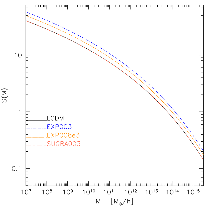
Figure 1: The mass variance $S$ (see equation 5) as a function of the halo mass. The different curves show the results for the different linear power spectra of the models considered in this work. Their shapes are independent of the cosmological model considered while the normalizations change depending on the linear power spectrum normalization and so on the corresponding $\sigma_{8}$.

In Fig. 2 we show the cumulative generalized formation redshift distribution in terms of the rescaled variable $w_{f}$ when the main halo progenitors assemble $90\%$, $50\%$, $10\%$ and $1\%$ of their $M_{200}$ mass at $z=0$. The data points represent the measurements in the $\mathrm{\Lambda}$CDM simulation considering all haloes at $z_{0}=0$ with mass larger than $M_{200}>5\times 10^{12}M_{\odot}/h$ (which means that systems are resolved with at least $40$ particles) and that never exceed along their growth histories more than $10\%$ of their mass at the present time. This ensures to consider only haloes that grow mainly hierarchically and do not fragment as a consequence of violent merging events. With respect to Giocoli et al. (2012b), in this case haloes are followed back in time considering $M_{200}$ as mass definition instead of $M_{vir}$ The solid curves show the best-fitting model of equation (12), while the dashed curves represent equation (10) modified as suggested by Giocoli et al. (2007).

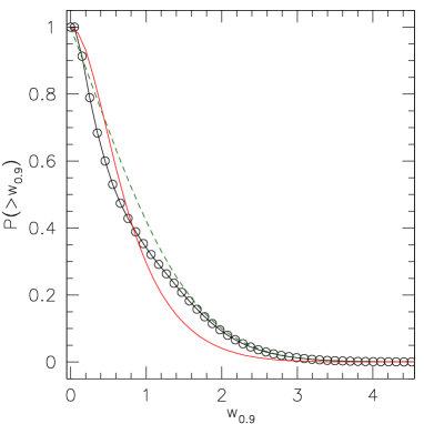
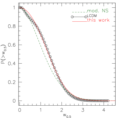
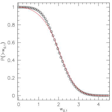
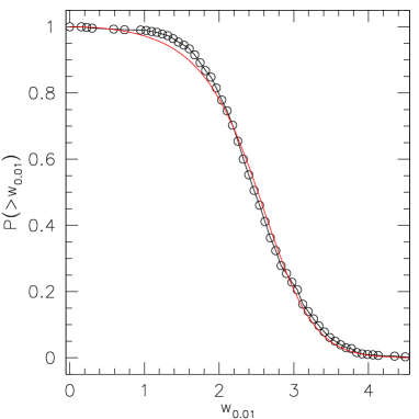
Figure 2: Cumulative generalized formation distribution, as a function of $w_{f}$, when the main halo progenitor assembles $90\%$ (top-left panel ), $50\%$ (top-right panel), $10\%$ (bottom-left panel) and $1\%$ (bottom-right panel) of its $M_{200}$ mass at redshift zero. The data points show the measurements for the $\Lambda$CDM simulation considering all haloes with at least $40$ particles. The dashed curve on the top panels refers to the model by Nusser & Sheth (1999) – valid only for $1/2<f\leq 1$, while the solid curve represents equation (12) with the best-fitting parameter $\alpha_{f}$. We recall that we consider only haloes that along their growth never exceed more than $10\%$ their mass at the present time.

From the figure we notice that – since at $z=0$ the value of $M_{200}$ is smaller than that of $M_{vir}$ – following the merger tree back in time in terms of $M_{200}$ results in a value of $z_{f}$ typically higher than that obtained by following back the tree in terms of $M_{vir}$ (see Giocoli et al., 2012b, or the Appendix A where we show the same cumulative distribution of formation redshift following the haloes in term of their virial mass for the $\mathrm{\Lambda}$CDM run).

In Fig. 3 we show the best-fitting $\alpha_{f}$ as a function of $f$. The open circles show the best fit to the $\mathrm{\Lambda}$CDM simulation measurement for different values of the assembled mass fraction, while the solid line refers to the best fit to the data given by:

$$\alpha_{f}=\dfrac{1.365}{f^{0.65}}\,\mathrm{e}^{-2f^{3}}\,.$$ (15)

Finally, the shaded regions represent the 1$\sigma$ and 2$\sigma$ contours of $\Delta\chi^{2}$, where $\chi^{2}(\alpha_{f})=\sum_{i}[P_{i}-P(>w_{i,f},\alpha_{f})^{2}]$.

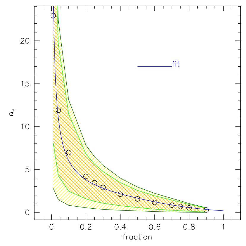
Figure 3: Dependence of $\alpha_{f}$, the free parameter in equation (12), on the mass fraction $f=M_{200}(z_{f})/M_{200}(0)$ assumed at the formation. The shaded regions represent the 1$\sigma$ and 2$\sigma$ contours. The blue curve represents the best-fitting relation.

5.2 Generalized formation redshift and mass accretion history

The hierarchical model predicts that small haloes tend to form at higher redshift and then merge together forming the larger ones. The halo collapse happens when a density fluctuation exceeds the critical value predicted by the spherical collapse model. Typically, within a $\Lambda$CDM Universe fluctuations in a density field with a larger amplitude collapse earlier. This can be rephrased considering two identical CDM initial density fields but with different normalization parameters $\sigma_{8}$: haloes in the Universe with higher $\sigma_{8}$ will collapse earlier than those in the Universe with lower $\sigma_{8}$. This also results in the fact of same mass haloes being more concentrated in a Universe with a larger value of $\sigma_{8}$ (Macciò et al., 2008). In what follows we will try to understand if this holds also for different cosmological scenarios, i.e. if the mass accretion history measured in numerical simulations of cDE can be reproduced by the MAH model built for $\Lambda$CDM only by suitably changing the linear power spectrum normalization $\sigma_{8}$.

In the upper part of each panel of Fig. 4 we show the median formation redshift as a function of the halo mass, considering $f=0.9$, 0.5, 0.1, 0.01 as assembled mass fractions. The open circles show the median of the measurements in the $\mathrm{\Lambda}$CDM simulation and the shaded region encloses the first and the third quartiles of the distribution at fixed halo mass. On average a present-day cluster size halo with mass of $10^{14}M_{\odot}/h$ assembles $90\%$ of its mass at $z=0.2$, $50\%$ at 0.7 and $1\%$ at approximately $z=4$. The data points in the lower part of each panel represent the differences of the median measured in the three cDE models with respect to the $\mathrm{\Lambda}$CDM one; the three curves show the model of the $z_{f}-M_{200}$ relation rescaled with respect to the $\mathrm{\Lambda}$CDM model computed using the formalism described in the previous section.

It is important to underline that in order to build the MAH model in the three cDE cosmologies we need to know the initial density fluctuation field to compute $S(M)$, and the redshift evolution and the growth of the perturbations given by $\delta_{c}(z)$ and $\Delta_{+}(z)$. For the definition of $S(M)$, we use for the three cDE models their corresponding linear power spectra, that are obtained from the $\mathrm{\Lambda}$CDM one by renormalizing the latter adopting the different values of $\sigma_{8}$ characterizing each cDE model (see Table 1). Since the purpose of this work is to understand if the MAH of the cDE simulations can be obtained from the $\mathrm{\Lambda}$CDM by rescaling $\sigma_{8}$ only, we adopt for the definitions of both $\delta_{c}(z)$ and $D_{+}$ the ones obtained for the latter model. From Fig. 4, we notice that only for $f=0.5$ the three cDE results are quite in agreement with the MAH model where the power spectrum normalization changes. Among them, since the SUGRA003 model has the same $\sigma_{8}$ of $\mathrm{\Lambda}$CDM, we would expect to find a formation-redshift relation quite similar to the latter. However, this is clearly not the case due to the markedly different growth of SUGRA003 as compared to $\Lambda$CDM. For $f=0.9$ and $f=0.5$ haloes in the SUGRA003 model form typically at the same redshift as in the $\mathrm{\Lambda}$CDM run, while for $f=0.1$ and $0.01$ the difference appears of the order of $10\%$. We underline also that for the two models EXP003 and EXP008e3 the halo formation redshifts are higher for any $f$ than those measured in $\mathrm{\Lambda}$CDM for the same mass haloes at $z=0$.

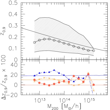
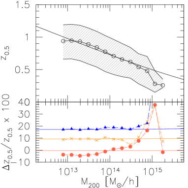
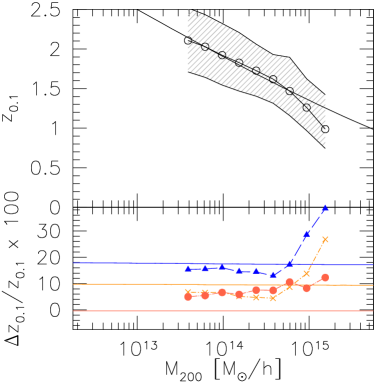
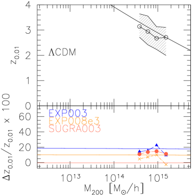
Figure 4: Top panels: median formation redshift-mass relation for haloes identified at $z_{0}=0$ in the $\Lambda$CDM simulation. The shaded region encloses the quartiles of the distribution at fixed halo mass. The solid line represents the prediction derived using the modified version of the Giocoli et al. (2012b) mass accretion history model. Bottom panels: differences with respect to the $\Lambda$CDM model for the three cDE models. The lines represent the predictions obtained from the modified model by Giocoli et al. (2012b) by changing the definition of $S(M)$ for each cosmology only.

To better understand how on average haloes assemble as a function of redshift, we show in Fig. 5 the median mass accretion history for three different mass bins at $z=0$ by defining $\Psi$ as the logarithm of the final assembled mass fraction:

$$\Psi(z)=\log\left[\dfrac{M_{200}(z)}{M_{200}(0)}\right]=\log(f)\,.$$ (16)

In the top panels we show the measurements for three different final halo mass bins at the present time in the $\mathrm{\Lambda}$CDM simulation. The shaded region encloses the first and the third quartiles of the distribution at fixed halo mass fraction. The solid curve represents the model built using equation (13) for different values of the assembled halo mass fraction $0<f<1$.

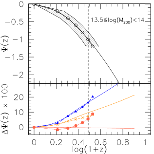
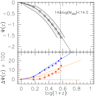
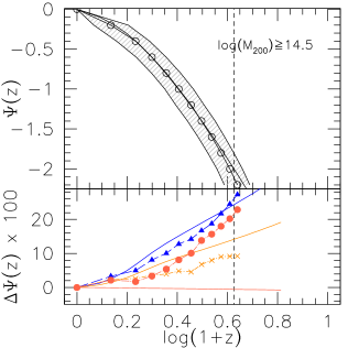
Figure 5: Median mass accretion history of main halo progenitors. In the top part of each panel we show the results from the $\mathrm{\Lambda}$CDM simulation for three different initial mass bins, where the shaded region encloses the quartiles of the distribution at fixed halo mass fraction assembled. In each panel, the solid curve represents the prediction from eq. (13). The bottom part of each panel shows the residuals with respect to the $\mathrm{\Lambda}$CDM simulation measurements of the three cDE models together with the residuals for the theoretical predictions changing $S(M)$ in the mass accretion history model. Point style as in Fig. 4.

The model predicts for the $\mathrm{\Lambda}$CDM run a MAH that is in agreement within a few percent with the numerical simulation measurements both down to very small values of the assembled mass fraction and up to high redshifts. In the bottom panels we show the percentage difference of the MAH measured in EXP003, EXP008e3 and SUGRA003 with respect to the one in $\mathrm{\Lambda}$CDM. In the figure, the different data points are the same as in Fig. 4. The three solid curves represent the difference of MAH models changing the linear power spectrum definition with respect to the $\mathrm{\Lambda}$CDM model. Since the SUGRA003 model has almost the same linear power spectrum normalization of the $\mathrm{\Lambda}$CDM, the MAH model predicts the same growth of the latter, in contrast with what is measured in the numerical simulation. For EXP003 the halo growth is quite well captured changing the linear power spectrum normalization in our model - and is therefore fully degenerate with $\sigma_{8}$. However, for EXP008e3 the model fails for large haloes and high redshift.

6 The Halo Structural Properties

6.1 Halo concentrations

One of the most important result obtained through N-body simulations of structure formation is that the CDM density distribution in collapsed haloes tends to follow a universal profile. Both for small and large mass haloes the density profile is well described by the Navarro-Frenk-White (NFW, Navarro et al., 1997) relation that reads as:

$$\rho(x)=\dfrac{\rho_{s}}{x(1+x)^{2}}\,,$$ (17)

where $x\equiv r/r_{s}$, $r_{s}\equiv R_{200}/c_{200}$ is the scale radius where the logarithmic slope of the density profile approaches $-2$, $\rho_{s}$ is the density enclosed within the scale radius, and $c_{200}$ is the halo concentration parameter. Denoting with $R_{200}$ the radius enclosing $M_{200}$ we can write:

$$\rho_{s}=\dfrac{M_{200}}{4\pi r_{s}^{3}}\left[\ln(1+c_{200})-\dfrac{c_{200}}{1+c_{200}}\right]^{-1}\,.$$ (18)

To characterize the halo concentration in the numerical simulations we use the same approach adopted by Springel et al. (2008) and Cui et al. (2012): defining $V_{max}$ as the maximum circular velocity of a halo and $r_{max}$ as the radius at which this velocity is attained so we can write:

$$\dfrac{\rho_{s}}{\rho_{crit}} = \dfrac{200}{3}\dfrac{c_{200}^{3}}{\ln(1+c_{200})-c_{200}/(1+c_{200})}$$ (19)

$$= 14.426\left(\dfrac{V_{max}}{H(z)\,r_{max}}\right)^{2}\,,$$

where $\rho_{crit}$ represents the critical density of the Universe. In Fig. 6 we show the distribution function of the maximum circular velocity and of the radius at which it is attained for all haloes that at the present time are more massive than $5\times 10^{13}M_{\odot}/h$. Since to faithfully determine the halo concentration a minimum number of particles is required (Neto et al., 2007), for this analysis we consider only haloes more massive than $5\times 10^{13}M_{\odot}/h$; this lower limit ensures that the haloes are resolved with at least $850$ particles. We notice that while the haloes in EXP003 and EXP008e3 have values of $V_{max}$ and $R_{max}$ that are not much different from the corresponding haloes in the $\mathrm{\Lambda}$CDM, the haloes in SUGRA003 are more compact and typically have a higher maximum circular velocity that is attained at a smaller radius than in $\mathrm{\Lambda}$CDM; as we will see later on, this corresponds to more concentrated haloes in SUGRA003 at $z=0$ than in the other three cosmological models.

In the context of the CDM hierarchical structure formation scenario, halo concentrations are thought to be reminiscent of the cosmic mean density at the time of collapse, thereby resulting in smaller objects having on average higher concentrations due to their earlier formation epoch. Consistently with this picture, clusters of galaxies have the lowest concentrations – typically of the order of $\sim 4$ – being the last collapsed structures in the Universe. At fixed redshift and halo mass the concentration tends to be larger for haloes that assemble their mass earlier; this also corresponds to haloes that are, on average, more relaxed. Neto et al. (2007), Macciò et al. (2007, 2008) and De Boni et al. (2012) have shown that including unrelaxed haloes in the sample results in a $c-M$ relation with a lower normalization and a larger scatter.

Several studies based on the analysis of numerical simulations have shown that halo structural properties are mainly related to the halo mass accretion history, and so to their environment (Gao et al., 2004; Sheth & Tormen, 2004; Gao et al., 2008). Not only do less massive haloes possess a higher concentration but typically also a smaller mass fraction in substructures (De Lucia et al., 2004; van den Bosch et al., 2005; Giocoli et al., 2010a). In particular, the $c-M$ models by Navarro et al. (1997) and Bullock et al. (2001) rely on the idea that the central density of the haloes reflects the mean density of the Universe at a time when the central region of the halo was accreting matter at a high rate. Zhao et al. (2009) define this epoch when the main halo progenitor first containing $4\%$ of the final mass.

In order to understand how halo concentration correlates with the accretion history, in what follows we study the correlation between $c_{200}$ and two conventional markers of the halo MAH: $z_{0.5}$ i.e. the redshift at which the main halo progenitor assembles half of its final mass (we will denote with $t_{0.5}$ the corresponding cosmic time) and $z_{0.04}$ (at which corresponds $t_{0.04}$), i.e. the redshift at which it assembles $4\%$ of its mass.

In Fig. 7 we show the correlation between the halo concentration and $t_{0}/t_{0.5}$ where $t_{0}$ represents the time at which the halo is considered – in our case $z_{0}=0$. In each panel we show the measurements for all haloes more massive than $5\times 10^{13}M_{\odot}/h$ in the $\mathrm{\Lambda}$CDM and the three cDE models. The data points with error bars show the median of the correlation and the quartiles of the distribution at fixed $t_{0}/t_{0.5}$. In the top-left panel the solid black line shows the least-square fit to the $\mathrm{\Lambda}$CDM measurements, and the dotted red curve represents the following best-fit power law-relation obtained by minimizing the scatter:

$$c_{200}=4\left[1+\left(\dfrac{t_{0}}{1.5t_{0.5}}\right)^{5.2}\right]^{1/5}\,.$$ (20)

Equation (20) is similar to the one proposed by Zhao et al. (2009). These two relations are also overplotted in the other panels. In each panel the grey histograms on the $x$ and the $y$ axis represent the distributions of $t_{0}/t_{0.5}$ and $c_{200}$, respectively. The different line types in the EXP003, EXP008e3 and SUGRA panels show the least-squares fit to the corresponding measurements. In Table 3 we summarize these results and give an estimate of the rms of the data points for the different numerical simulation results defined as:

$$\mathrm{rms}=\sqrt{\sum_{i=1}^{N}\dfrac{\left(\log(c_{i})-\log(c_{model})\right)^{2}}{N}}\,.$$ (21)

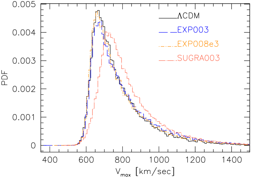
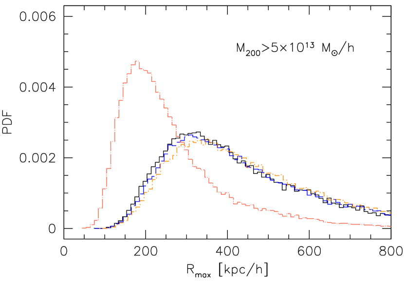
Figure 6: Distribution function of maximum circular velocity (top panel) and of the radius at which this is reached (bottom panel) for all haloes at $z=0$ with masses larger than $5\times 10^{13}M_{\odot}/h$ in the four cosmological simulations.

Table 3: Rms of the data with respect to the models of Fig. 7.

model	eq. (20)	$\mathrm{\Lambda}$CDM least-squares	least-squares	least-square values
				slope, zero point
$\mathrm{\Lambda}$CDM	0.128	0.127	-	0.870, 0.503
EXP003	0.132	0.134	0.128	0.748, 0.506
EXP008e3	0.133	0.135	0.128	0.749, 0.488
SUGRA003	0.255	0.254	0.135	0.897, 0.704

Zhao et al. (2009) have shown that the halo concentration has a strong correlation with the time $t_{0.04}$ at which the main halo progenitor assembles for the first time $4\%$ of its mass, in the idea that typically haloes acquire a concentration of $4$ when they assemble $4\%$ of their mass. From their measurements, the best-fitting relation between the concentration and $t_{0.04}$ reads as:

$$c_{vir}=4\left[1+\left(\dfrac{t_{0}}{3.75t_{0.04}}\right)^{8.4}\right]^{1/8}\,,$$ (22)

where $c_{vir}$ represents the ratio between the scale radius $r_{s}$ and the virial radius $R_{vir}$. We recall that Zhao et al. (2009) define $R_{vir}$ such that it encloses an overdensity $\Delta_{vir}$ according to the spherical collapse model, with respect to which they also define the virial mass $M_{vir}$. In Fig. 8 we show the median of the correlation between $c_{200}$ and $t_{0}/t_{0.04}$ for the measurements in the four N-body simulations used in this work. The short-dashed lines show equation (22), that we recall is valid for the $c_{vir}$ and $M_{vir}$ definitions. In the top-left panel the solid line shows our best relation obtained modifying the Zhao et al. (2009) fitting function to be valid for the $c_{200}$ and the $M_{200}$ definitions, which reads as:

$$c_{200}=4\left[1+\left(\dfrac{t_{0}}{3.2t_{0.04}}\right)^{8}\right]^{1/13}\,.$$ (23)

These two curves are also shown in the other three panels of Fig. 8. The different curve types in each panel show equation (23) renormalized (see Table 4) in order to best-fitting the data points; we denote with $A$ the re-normalization parameter to fit the corresponding data. In Table 4 we summarize the results of Fig. 8 together with the rms with respect to the different models.

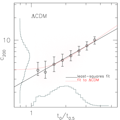
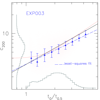
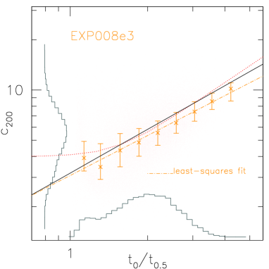
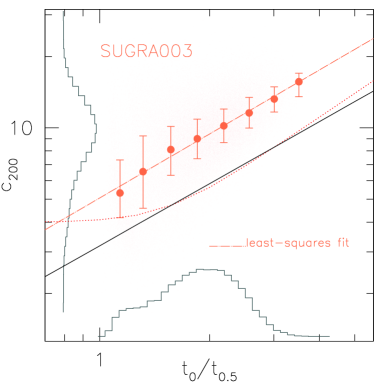
Figure 7: Correlation between the concentration and the formation time when the main halo progenitor assembles $50\%$ of the mass at $z_{0}=0$. The four panels refer to the different cosmological models. In each panel the points with the error bars show the median with the two quartiles. Solid (black) and dotted lines in all panels are the same and represent the least-square fit to the haloes in the $\Lambda$CDM simulation and equation (20) respectively. The different line types in the panels referring to the cDE models represent the corresponding least-square fit to their data points.

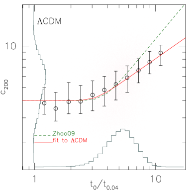
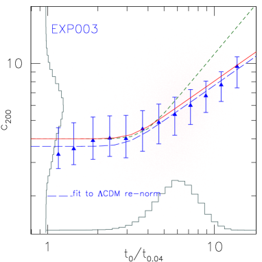
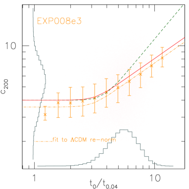
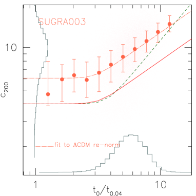
Figure 8: Correlation between the concentration and the formation time when the main halo progenitor assembles $4\%$ of the mass at $z_{0}=0$. Dashed and solid curves in all panels show equations (22) and (23). In the three cDE models the different line type curves show equation (23) renormalized to best-fitting the corresponding data points.

Table 4: Rms of the measured concentration (from the second to the forth columns) and least-squares fit parameters of the data (fifth column) with respect to the models shown in Fig. 8.

	$|$		rms with respect to		$|$
model	$|$	Zhao et al. (2009)	eq. (23)	eq. (23)$\times A$	$|$	$\log(A)$
$\mathrm{\Lambda}$CDM	$|$	0.152	0.143	-	$|$	-
EXP003	$|$	0.178	0.148	0.143	$|$	-0.04
EXP008e3	$|$	0.168	0.147	0.143	$|$	-0.05
SUGRA003	$|$	0.211	0.241	0.143	$|$	0.19

Using the MAH model previously presented in this work and considering the correlations between $c_{200}$ and $t_{0.5}$ and $c_{200}$ and $t_{0.04}$, it is possible to estimate the concentration-mass relation model, in the following way. Given a mass $M_{200}$ at redshift $z_{0}$, we can estimate the redshift at which the main halo progenitor assembles half (or $4\%$) of its mass by using equation (13), and then the corresponding cosmic time by integrating over the scale factor $a=1/(1+z)$ the inverse of the Hubble constant $1/H(a)$, from which we can obtain $c_{200}$. In Fig. 9 we show the median of the concentration-mass relation for all haloes more massive than $5\times 10^{13}M_{\odot}/h$ at redshift $z_{0}=0$. The data points in both right and left panels are the same. In the top panels they represent the median of the concentration-mass relation measured in the $\mathrm{\Lambda}$CDM simulation, and the shaded region encloses the first and the third quartiles of the distribution at fixed mass. In the bottom panels we show the differences of the median of the measurements in the three cDE models with respect to the $\mathrm{\Lambda}$CDM one.

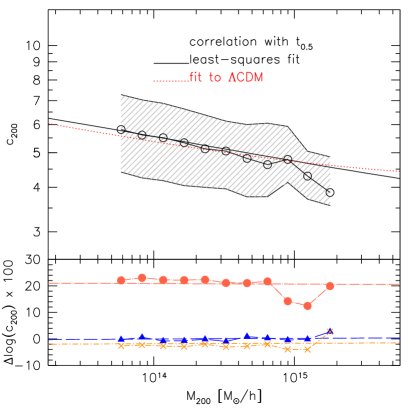
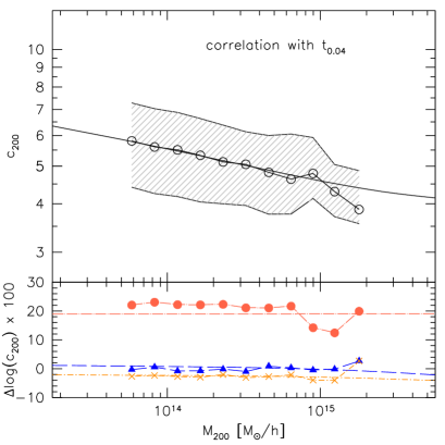
Figure 9: Concentration-mass relation at $z_{0}=0$. The data points show the median $c-M$ relation measured in the $\mathrm{\Lambda}$CDM simulation and the shaded region encloses the quartiles. In the bottom part of each panel the points show the differences of the $c-M$ measured in the three cDE simulations with respect to the $\mathrm{\Lambda}$CDM one. In the left-top panel the two solid curves show the $c-M$ prediction using equation (20) and the least-squares relation $c_{200}-t_{0}/t_{0.5}$. In the bottom left panel the curves show for each model the residuals of the $c-M$ prediction from the least-squares fit in $c_{200}-t_{0}/t_{0.5}$ relation with respect to the one for $\mathrm{\Lambda}$CDM. In the top-right panel the $c-M$ prediction is from equation (23) and in the bottom panel the curves are the residuals of the predictions from renormalizing eq. (23).

In Table 5 we summarize the residuals of the $c-M$ estimates with respect to the different model predictions; the column l-s${}_{t_{0.5,\mathrm{\Lambda CDM}}}$ refers to the prediction made using the least-squares to the correlation $c_{200}$-$t_{0}/t_{0.5}$ for the $\mathrm{\Lambda CDM}$ cosmology while l-s${}_{t_{0.5}}$ refers to the prediction done with the least-squares fit to the corresponding cosmology.

Table 5: Rms of the measured concentration with respect to the $c-M$ relation model, as presented in the panels of Fig. 9.

	$|$			rms with respect to
model	$|$	eq. (20)	l-s${}_{t_{0.5,\mathrm{\Lambda CDM}}}$	l-s${}_{t_{0.5}}$	eq. (23)	eq. (23)$\times A$
$\mathrm{\Lambda}$CDM	$|$	0.153	0.154	-	0.154	-
EXP003	$|$	0.157	0.161	0.153	0.165	0.154
EXP008e3	$|$	0.156	0.161	0.152	0.163	0.151
SUGRA003	$|$	0.270	0.259	0.162	0.260	0.162

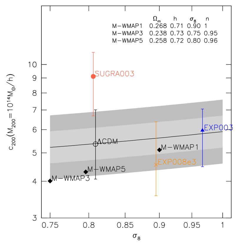
Figure 10: Concentration-$\sigma_{8}$ relation for a halo with mass $M_{200}=1\times 10^{14}M_{\odot}/h$ using the least-squares fit $c_{200}-t_{0}/t_{0.5}$. The colored data points show the median of the measurements in the simulations with the quartiles. For each simulation, we consider haloes within a logarithmic mass bin $\mathrm{d}\log(M)=0.001$ centered in $M_{200}=10^{14}M_{\odot}/h$. The three black data points labelled as M-WMAP1, M-WMAP3 and M-WMAP5 are the estimates obtained using the best-fitting relation at $z=0$ by Macciò et al. (2008) for the three corresponding numerical simulations.

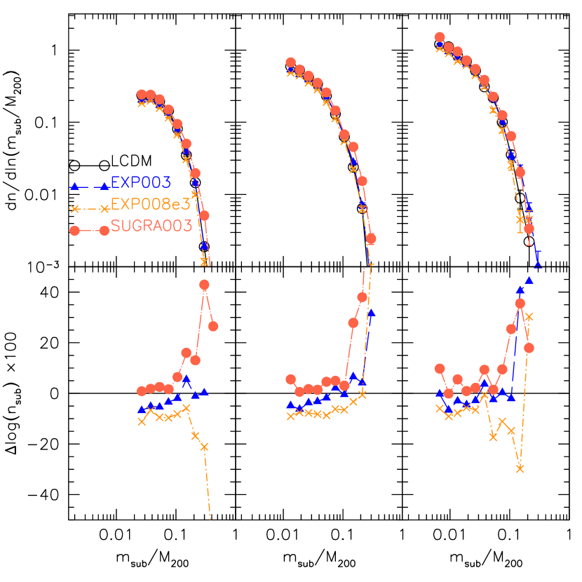
Figure 11: Subhalo mass function measured in the four cosmological simulations used in this work. The subhalo mass is rescaled with respect to the host halo mass $M_{200}$, and for each halo we have considered only subhaloes with a distance from the host halo centre smaller than $R_{200}$. In the bottom part of the figure we show the differences of the subhalo mass function with respect to the measurements done in the $\mathrm{\Lambda}$CDM simulation.

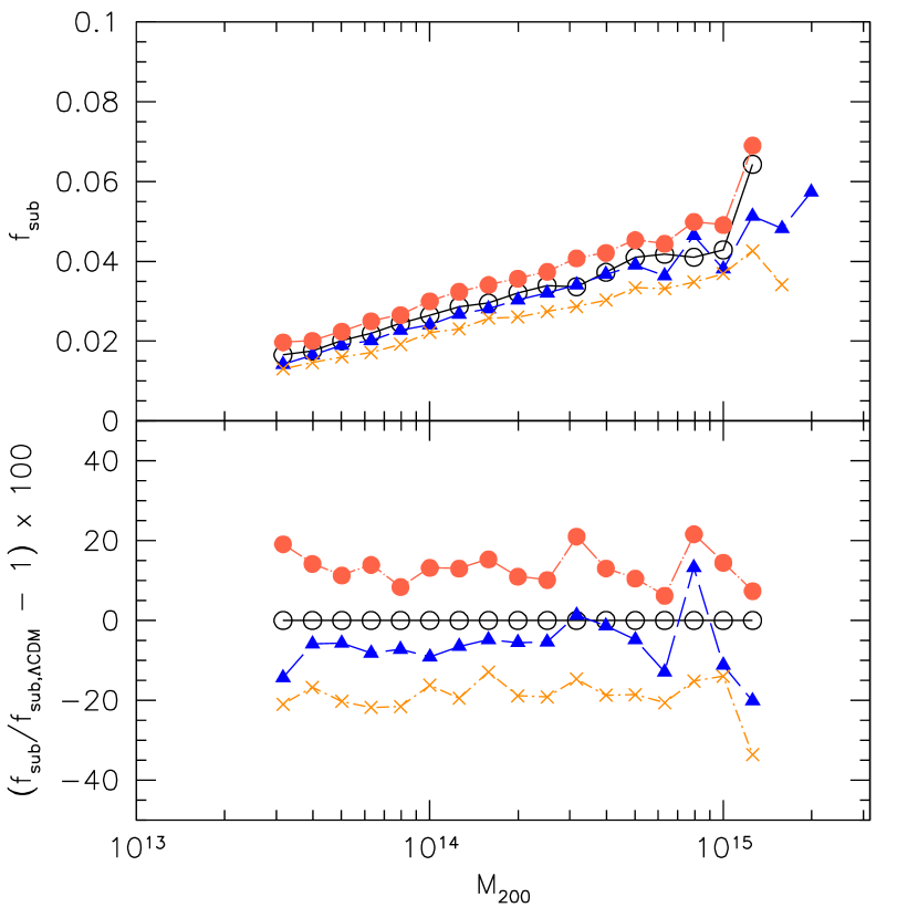
Figure 12: Mass fraction in substructures within $R_{200}$ as a function of the host halo mass. In the bottom part we show the differences of the mass fraction in substructures with respect to the $\mathrm{\Lambda}$CDM measurements.

Macciò et al. (2008) and Zhao et al. (2009) have shown that haloes in standard $\Lambda$CDM simulations with low values of $\sigma_{8}$ and/or $\Omega_{m}$ tend to possess a lower concentration due to their later formation epoch. In what follows we will try to understand if this is also the case in our non-standard cDE simulations, i.e we will enquire whether the concentration can be inferred from the $\mathrm{\Lambda}$CDM one by simply taking into account the different normalization of the linear matter power spectrum at $z=0$ within the standard MAH model.

From the analysis presented above, we have already noticed that even if the EXP003 and EXP008e3 models have a higher value of $\sigma_{8}$, the halo concentration is not too different from that measured for haloes of the same mass in the $\mathrm{\Lambda}$CDM model. Only the SUGRA003 haloes are found to have a significantly higher concentration, irrespectively of their value of $\sigma_{8}$ that is very similar to the one in the $\mathrm{\Lambda}$CDM run. These results are consistent with the previous findings of Cui et al. (2012).

In order to quantify to what extent halo concentrations are expected to change for different values of $\sigma_{8}$ within a $\Lambda$CDM cosmology, we plot in Fig. 10 the concentration-$\sigma_{8}$ prediction combining the least-squares fit $c_{200}-t_{0}/t_{0.5}$ and the MAH model for a halo with mass $M_{200}=1\times 10^{14}M_{\odot}/h$ as expected for $\mathrm{\Lambda}$CDM – with the same cosmological parameters of our $\mathrm{\Lambda}$CDM run – but with different values of $\sigma_{8}$. We take into account the change of $\sigma_{8}$ by renormalizing the mass variance such that:

$$S_{\sigma_{8}}(M)=\dfrac{\sigma_{8}^{2}}{0.809^{2}}S_{\mathrm{\Lambda CDM}}(M)\,.$$ (24)

Fixing all the other cosmological parameters, we notice that the larger $\sigma_{8}$ the larger is the halo concentration, as expected, reflecting the fact that haloes tend to form earlier. From the figure we can see that when $\sigma_{8}$ changes from 0.75 to 1 the halo concentration changes by $\sim 20\%$. The data points with the error bars show the median and the quartiles of $c_{200}$ for the same mass haloes measured in the four simulations at $z=0$; we consider a logarithmic mass bin $\mathrm{d}\log(M)=0.001$ centered in $M_{200}=10^{14}M_{\odot}/h$. The three data points M-WMAP1, M-WMAP3 and M-WMAP5 are the predictions based on the $c_{200}-M_{200}$ relations by Macciò et al. (2008) for the three cosmological models at $z=0$. The fact that the predictions from the relations by Macciò et al. (2008) shift down with respect to the solid curve reflects the smaller values for $\Omega_{m}$ adopted their simulations: $\Omega_{m,\mathrm{\Lambda CDM}}\gtrsim\Omega_{m,M-WMA1}>\Omega_{m,M-WMA5}>\Omega_{m,M-WMA3}$. From the figure we notice that haloes in EXP003 possess a higher concentration than in $\mathrm{\Lambda}$CDM, consistently with the higher value of $\sigma_{8}(z_{0})$ that characterizes the model (see Table 1).

However, the expected trend of $c_{200}$ as a function of $\sigma_{8}$ is not followed both in EXP008e3 and SUGRA003. This point represents a central result of the present work, and deserves a more detailed discussion. It is well known that standard cDE models are characterized by a suppression of the non-linear matter power spectrum with respect to what $\Lambda$CDM predicts for any given value of $\sigma_{8}$. This has been demonstrated both by running cDE N-body simulations with the same $\sigma_{8}$ (as done e.g. in Baldi, 2011a) and by comparing the non-linear matter power spectrum extracted from cDE N-body simulations normalized at $z_{\rm CMB}\approx 1100$ to the predictions of HALOFIT (Smith et al., 2003) for the corresponding values of $\sigma_{8}$ (see e.g. Baldi, 2012b). Such suppression is determined by the action of the “friction term” (see the discussion in Section 3 above) that for standard cDE models has the effect of suppressing the growth of nonlinear structures. Correspondingly, for a fixed value of $\sigma_{8}$ CDM haloes are found to be less concentrated in a cDE cosmology when compared with respect to $\Lambda$CDM (see e.g. Baldi et al., 2010; Baldi, 2011a; Li & Barrow, 2011). For more complex cDE models, like time-dependent couplings or the “bouncing” cDE scenario, the role played by the “friction term” is not so straightforward as the latter can change sign during the cosmic evolution or have a non-trivial interplay with the time evolution of the coupling itself. In such more general scenarios, halo concentrations at fixed $\sigma_{8}$ can be both higher and lower than in $\Lambda$CDM, depending on the specific model.

Among the models considered in the present work, the slight increase of halo concentrations for the standard EXP003 cDE model shows how the suppression associated to the “friction term” is compensated by the higher value of $\sigma_{8}$ of this cosmological model as compared to $\Lambda$CDM. Furthermore, the lower and higher values of halo concentrations with respect to what is predicted by the standard $\Lambda$CDM scenario, that are observed for the EXP008e3 and SUGRA003 models, respectively, show how the dynamical evolution of the DE scalar field can alter the structural properties of CDM haloes in a way that is clearly independent of the evolution of linear density perturbations. For instance, in the case of the “bouncing” cDE model (SUGRA003), halo concentrations significantly grow in time at low redshifts (as already found by Cui et al., 2012) due to the particular dynamics of the DE scalar field that inverts its direction of motion at $z_{\rm inv}\simeq 6.8$ thereby also changing the sign of the “friction” term $\beta_{c}\dot{\phi}$ (see Baldi, 2012a, for a more detailed discussion of the dynamics of “bouncing” cDE). The latter then acts as a dissipation term for virialized objects inducing an adiabatic contraction of halos that consequently evolve towards more concentrated virial configurations.

This direct relation between the dynamics of the underlying DE field and the formation and evolution of nonlinear structures offers the interesting prospect of using the formation history of CDM haloes and their structural properties to disentangle cDE effects from possible variations of cosmological parameters (as e.g. $\sigma_{8}$), of the linear galaxy bias, and of the mass of cosmic neutrinos (see e.g. La Vacca et al., 2009; Marulli et al., 2011).

6.2 Halo substructures

Studying the subhalo population in DM haloes extracted from a standard cosmological $\mathrm{\Lambda}$CDM simulation at $z=0$, Giocoli et al. (2010a) found that more concentrated haloes, forming at higher redshift, tend to possess on average less substructures above the same mass ratio $m_{sub}/M_{200}$. They have also stressed the fact that considering haloes with the same mass, the ones that form earlier not only possess a higher concentration, but also few subhaloes. This is because halo progenitors are accreted earlier, then spending more time in the potential well of the host halo, and thereby tend to lose a larger fraction of their initial mass (van den Bosch et al., 2005; Giocoli et al., 2008). To see if this phenomenology is also reflected in the cDE simulations considered in this work, we plot in Fig. 11 the subhalo mass function considering for each halo all substructures resolved by subfind with a distance from the host halo centre smaller than $R_{200}$. In the top part of the figure we show the subhalo mass function for three different host halo mass bin (as in Fig. 5) at $z=0$, while in the bottom one the differences with respect to the measurements in the $\mathrm{\Lambda}$CDM simulation. Since we have shown that haloes in SUGRA assemble earlier and are more concentrated than those in the $\mathrm{\Lambda}$CDM run, we would have expected them to possess less substructures, on the contrary to what is shown in the figure. Also the subhalo population in the EXP003 and EXP008e3 cosmologies does not reflect their mass accretion history. In these models, haloes possess less substructures than those in $\mathrm{\Lambda}$CDM since they form earlier, but even if in EXP003 haloes form earlier than those in EXP008e3 they are still found to host more substructures than in the latter model. This statement is further demonstrated in Fig. 12 where we show the halo mass fraction in subhaloes as a function of $M_{200}$. In the bottom part of the figure we show again the differences of the measurements in the cDE with respecto to the one in $\mathrm{\Lambda}$CDM: haloes in SUGRA (EXP008e3) are more (less) substructured than those in $\mathrm{\Lambda}$CDM by $\sim 15\%$ while the difference between EXP003 and $\mathrm{\Lambda}$CDM is only of the order of a few percent. We argue that the main reason why SUGRA003 (EXP008e3) possesses more (less) substructures at $z=0$ is that halo progenitors at any redshift $z<1$, which end up in present-day substructures, are more (less) concentrated than in $\mathrm{\Lambda}$CDM; so the gravitational heating and tidal stripping are less (more) efficient in disrupting the satellites.

7 Summary and Conclusions

Using state-of-the-art cosmological simulations for cDE models from the CoDECS Project we have studied how collapsed haloes grow as a function of the cosmic time, and how present-day systems acquire their structural properties. We summarize our study and main results as follows.

• We updated the model developed by Giocoli et al. (2012b) in the context of the extended-Press & Schechter (1974) formalism to be able to describe the halo mass accretion history of a $\mathrm{\Lambda}$CDM cosmology when haloes are identified by their $M_{200}$ mass (instead of $M_{vir}$), defined as the mass of the spherical region around the halo center enclosing an average density 200 times larger than the critical density of the Universe.

• By rescaling the MAH model with the normalization of the linear matter power spectrum for the different cDE runs, we noticed that the simulation results are reproduced quite well for small masses and low redshift. For galaxy cluster-size haloes and up to high redshifts, when less than $1\%$ of the present-day mass is assembled, the models and the simulation measurements differ by about $20\%$. Haloes at $z=0$ in the different cDE cosmologies (standard cDE, time-dependent cDE, and “bouncing” cDE) typically assemble their mass at higher redshift as compared to those in the standard $\mathrm{\Lambda}$CDM run.

• We studied the formation redshift $z_{f}$ for different fractions $f$ of the assembled mass: standard and time-dependent cDE show a systematically higher $z_{f}$ by $\sim 20$ and $\sim 10\%$, respectively, as compared to $\mathrm{\Lambda}$CDM. On the other hand haloes in our “bouncing” cDE cosmology have a formation redshift quite similar to those in $\mathrm{\Lambda}$CDM, for small $f$, while for large assembled fractions $z_{f}$ can also be higher than in $\mathrm{\Lambda}$CDM by up to $\sim 20\%$.

• Analyzing the correlation between the halo concentration and two typical formation times $t_{0.5}$ and $t_{0.04}$, we confirm that the usual correlation between halo formation time and halo concentration at $z=0$ (the earlier the formation time, the higher the concentration) still holds in cDE cosmologies. Generalizing the prediction for $\mathrm{\Lambda}$CDM we provide some fitting functions for such correlations also in cDE models. In particular, in our “bouncing” cDE scenario haloes are very concentrated at $z=0$, inconsistently with the correlation expected for standard cosmologies (Cui et al., 2012). Such structural properties could produce very compact and luminous galaxies located in the centre of haloes and also galaxy clusters that are very efficient for strong lensing.

• Considering the correlation between $c_{200}$ and the time at which the main halo progenitor assembles for the first time half of its mass, we have confirmed that for standard $\mathrm{\Lambda}$CDM cosmologies the concentration is a monotonic function of $\sigma_{8}$: in particular for a cluster-size halo the change in concentration between two $\mathrm{\Lambda}$CDM cosmologies with $\sigma_{8}=0.75$ and $\sigma_{8}$ = 1 is of about $20\%$. Moving to cDE cosmologies, we have shown that only the standard cDE run, characterized by an exponential self-interaction potential and a constant coupling, is found to be in agreement with such predictions, while both cDE models with a time-dependent coupling and the “bouncing” cDE model are not found to be consistent with the expected evolution of halo concentrations with $\sigma_{8}$. This inconsistency offers the interesting prospect of disentangling the effects of dark interactions from the variation of standard cosmological parameters using the evolution of halo concentrations (Giocoli et al., 2012c).

• The standard mass accretion history model is also found to be not directly applicable to predict the subhalo population of the host haloes at $z=0$ within cDE cosmologies. In fact, if we generalize to the cDE simulations the statements by Gao et al. (2004), van den Bosch et al. (2005), and Giocoli et al. (2008) - valid for standard $\mathrm{\Lambda}$CDM - that haloes with a higher formation redshift typically possess less substructures, we would expect to find more substructures in $\mathrm{\Lambda}$CDM than in all our cDE models at any fixed halo mass. On the contrary, we find that the trend is actually reversed, with haloes of the same mass having $\sim 15\%$ more substructures within $R_{200}$ in the “bouncing” cDE run than in $\mathrm{\Lambda}$CDM, while haloes forming within a time-dependent cDE cosmology have less substructures by the same amount, while haloes in standard cDE are roughly consistent with their higher formation redshift and concentration but have slightly few substructures then in $\mathrm{\Lambda}$CDM. We argue that the higher concentration and the larger number of clumps in the SUGRA003 model are due to the fact haloes formed when the average density of the universe was larger, and the difference in the average density between the formation time of the small halos and the larger ones was also larger than in the in $\mathrm{\Lambda}$CDM. This makes satellites not only more concentrated than in thoes in $\mathrm{\Lambda}$CDM, but also more concentrated relative to the host halos: the subhalos then tend to survive tidal striping for longer time. In summary, while in standard $\mathrm{\Lambda}$CDM simulation – independently of the small scale behaviour of the linear power spectrum used to generate the initial conditions (Schneider et al., 2012) – the concentration-mass relation is expected to prove the halo formation time, the subhalo abundance as a function of the host halo mass validate the dynamical friction and the tidal stripping (van den Bosch et al., 2005).

To conclude, in the present work we have performed a detailed analysis of the mass accretion history of collapsed haloes in a sample of coupled Dark Energy cosmologies including different choices of the Dark Energy self-interaction and coupling functions. We have studied how haloes acquire their structural properties along the cosmic time and tested whether it is possible to attribute the detected differences with respect to the standard $\mathrm{\Lambda}$CDM case to the different linear power spectrum normalization. Interestingly, we found that this is not possible for all coupled Dark Energy models, and we identified which observables allow to break such a degeneracy. Finally, we have investigated by how much halo concentration and subhalo abundance deviate from $\mathrm{\Lambda}$CDM for the three coupled Dark Energy models included in our simulations set. In particular, we showed that the unexpected high concentration and clumpiness of haloes make the “bouncing” coupled Dark Energy model particularly interesting in the context of both weak and strong gravitational lensing. We intend to study the possibility of distinguishing such models from $\mathrm{\Lambda}$CDM using lensing data in future work.

Appendix A Mass Accretion History in terms of the Virial Mass for the $\mathrm{\Lambda}$CDM simulation

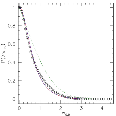
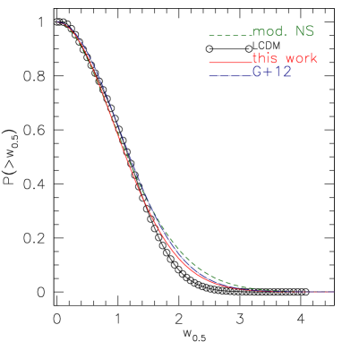
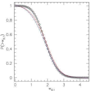
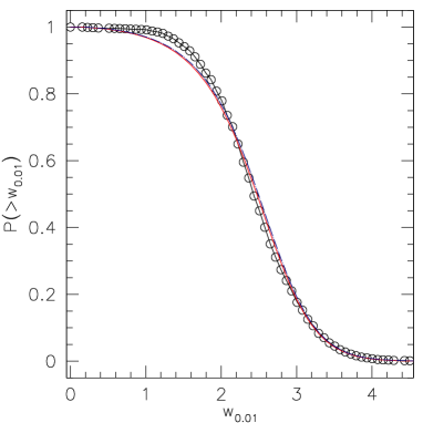
Figure 13: As Fig. 2 but in terms of $M_{vir}$.

In this Appendix we show that the MAH model built following back in time the haloes in the $\mathrm{\Lambda}$CDM simulation in terms of their virial mass $M_{vir}$ is in perfect agreement with the results obtained by Giocoli et al. (2012b). In Fig. 13 we show the cumulative generalized formation redshift distribution when $90\%$, $50\%$, $10\%$ and $1\%$ of the halo mass is assembled in term of the universal variable $w_{f}$. We compute the redshift at which the main halo progenitor assembles a fraction $f$ of its mass at $z=0$ interpolating its mass accretion history along the different simulation snapshots, and then compute $w_{f}=\left(\delta_{c}(z_{f})-\delta_{c}(z_{0})\right)/\sqrt{S(fM_{vir})-S(M_{vir})}$. The solid line in the figure shows equation (12) with the best-fitting value of $\alpha_{f}$. The dashed curve refers to the relation by Nusser & Sheth (1999) modified as proposed by Giocoli et al. (2007) and the dot-dashed curve equation (12) with the $\alpha_{f}-f$ relation by Giocoli et al. (2012b). We notice that our best-fitting is in very good agreement with what found by Giocoli et al. (2012b), and does not depend on the different cosmological parameters of the simulation since $w_{f}$ is a universal variable (Press & Schechter, 1974; Bond et al., 1991; Lacey & Cole, 1993, 1994). The small differences can be traced back to the different code used to run the two numerical simulations and to do the post processing analyses. While HYDRA (Couchman et al., 1995) and GADGET (Springel et al., 2001a) have been used for the GIF2 simulation studied by Giocoli et al. (2012b), a modified version of GADGET2 (Springel, 2005) developed to include all the additional physical effects that characterize cDE models (Baldi et al., 2010) has been run four our $\mathrm{\Lambda}$CDM simulation. For the post-processing analyses Giocoli et al. (2012b) have adapted and run the pipeline presented by Tormen et al. (2004), while here we have run the codes by Springel et al. (2001a) and Boylan-Kolchin et al. (2009). We recall the reader also on the fact that the GIF2 is a pure DM simulation while the CoDECS presents a baryon fluid with no hydrodynamic treatment included.

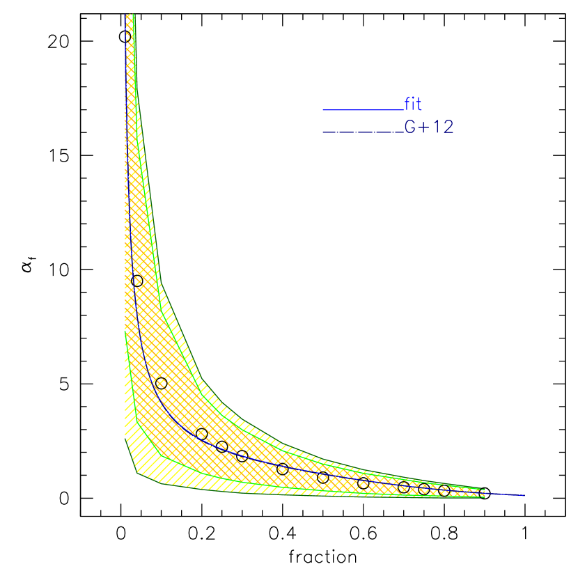
Figure 14: As Fig. 3 but in terms of $M_{vir}$.

In Fig. 14 we show the correlation between the free parameter of the MAH model $\alpha_{f}$ and the assembled mass fraction. The data points represent the best-fitting values obtained fitting the cumulative formation redshift distribution for different values of $f$; the shaded region encloses 1$\sigma$ and 2$\sigma$ contours around them. In the figure, the solid curve represents the following relation:

$$\alpha_{f}=\dfrac{0.837}{f^{0.7}}\,\mathrm{e}^{-2f^{3}}\,,$$ (25)

while the dot-dashed one is for:

$$\alpha_{f}=\dfrac{0.815}{f^{0.707}}\,\mathrm{e}^{-2f^{3}}\,,$$ (26)

as found by Giocoli et al. (2012b). The two relations for the $\mathrm{\Lambda}$CDM runs are in perfect agreement confirming the fact that the MAH model can be generalized for any $\mathrm{\Lambda}$CDM cosmology, independently of the cosmological parameters.

Appendix B Publicly available Merger Tree files on the CoDECS database

The merger trees of the different L-CoDECS simulations used to perform the analysis discussed in the present paper have been produced using a linking algorithm outlined in Springel et al. (2005) and Springel et al. (2008). With such algorithm, we produced a single merger tree file for each cosmological model of the L-CoDECS suite (i.e. even for those models that have not been considered in the present paper).

As an extension of the public CoDECS database, we hereby release the merger tree files that are now directly available at the CoDECS website (http://www.marcobaldi.it/CoDECS). These are unformatted binary files with an average size of about 10 Gb, and detailed instructions on how to read and use the data can be found on the CoDECS guide (version 2.0) that can also be directly downloaded from the CoDECS website.

The access to these files is subject to the same terms of use that apply to the whole CoDECS public database.

References

- Amendola (2000) Amendola L., 2000, Phys. Rev., D62, 043511
- Amendola (2004) Amendola L., 2004, Phys. Rev., D69, 103524
- Amendola et al. (2012) Amendola L., Appleby S., Bacon D., et al., 2012, ArXiv e-prints
- Amendola et al. (2008) Amendola L., Baldi M., Wetterich C., 2008, Phys.Rev.D, 78, 2, 023015
- Baldi (2011a) Baldi M., 2011a, MNRAS, 414, 116
- Baldi (2011b) Baldi M., 2011b, MNRAS, 411, 1077
- Baldi (2012a) Baldi M., 2012a, MNRAS, 420, 430
- Baldi (2012b) Baldi M., 2012b, MNRAS, 422, 1028
- Baldi et al. (2010) Baldi M., Pettorino V., Robbers G., Springel V., 2010, MNRAS, 403, 1684
- Bartelmann & Schneider (2001) Bartelmann M., Schneider P., 2001, Physics Reports, 340, 291
- Bertotti et al. (2003) Bertotti B., Iess L., Tortora P., 2003, Nature, 425, 374
- Beynon et al. (2012) Beynon E., Baldi M., Bacon D. J., Koyama K., Sabiu C., 2012, Mon.Not.Roy.Astron.Soc., 422, 3546
- Bond et al. (1991) Bond J. R., Cole S., Efstathiou G., Kaiser N., 1991, ApJ, 379, 440
- Boylan-Kolchin et al. (2009) Boylan-Kolchin M., Springel V., White S. D. M., Jenkins A., Lemson G., 2009, MNRAS, 398, 1150
- Brax & Martin (1999) Brax P., Martin J., 1999, Phys. Lett., B468, 40
- Bryan & Norman (1998) Bryan G. L., Norman M. L., 1998, ApJ, 495, 80
- Bullock et al. (2001) Bullock J. S., Kolatt T. S., Sigad Y., et al., 2001, MNRAS, 321, 559
- Cacciato et al. (2012) Cacciato M., Lahav O., van den Bosch F. C., Hoekstra H., Dekel A., 2012, MNRAS, 426, 566
- Caldera-Cabral et al. (2009) Caldera-Cabral G., Maartens R., Urena-Lopez L. A., 2009, Phys. Rev., D79, 063518
- Cooray & Sheth (2002) Cooray A., Sheth R., 2002, Physics Reports, 372, 1
- Couchman et al. (1995) Couchman H. M. P., Thomas P. A., Pearce F. R., 1995, ApJ, 452, 797
- Cui et al. (2012) Cui W., Baldi M., Borgani S., 2012, MNRAS, 424, 993
- Damour et al. (1990) Damour T., Gibbons G. W., Gundlach C., 1990, Phys. Rev. Lett., 64, 123
- Davis et al. (1985) Davis M., Efstathiou G., Frenk C. S., White S. D. M., 1985, ApJ, 292, 371
- De Boni et al. (2012) De Boni C., Ettori S., Dolag K., Moscardini L., 2012, MNRAS, 218
- De Felice & Tsujikawa (2010) De Felice A., Tsujikawa S., 2010, Living Rev.Rel., 13, 3
- De Lucia et al. (2004) De Lucia G., Kauffmann G., Springel V., et al., 2004, MNRAS, 348, 333
- Despali et al. (2012) Despali G., Tormen G., Sheth R. K., 2012, ArXiv e-prints
- Eke et al. (1996) Eke V. R., Cole S., Frenk C. S., 1996, MNRAS, 282, 263
- Farrar & Peebles (2004) Farrar G. R., Peebles P. J. E., 2004, ApJ, 604, 1
- Frenk et al. (1983) Frenk C. S., White S. D. M., Davis M., 1983, ApJ, 271, 417
- Frenk et al. (1990) Frenk C. S., White S. D. M., Efstathiou G., Davis M., 1990, ApJ, 351, 10
- Gao et al. (2008) Gao L., Navarro J. F., Cole S., et al., 2008, MNRAS, 387, 536
- Gao & White (2007) Gao L., White S. D. M., 2007, MNRAS, 377, L5
- Gao et al. (2004) Gao L., White S. D. M., Jenkins A., Stoehr F., Springel V., 2004, MNRAS, 355, 819
- Giocoli et al. (2010) Giocoli C., Bartelmann M., Sheth R. K., Cacciato M., 2010, MNRAS, 408, 300
- Giocoli et al. (2012a) Giocoli C., Meneghetti M., Bartelmann M., Moscardini L., Boldrin M., 2012a, MNRAS, 421, 3343
- Giocoli et al. (2012c) Giocoli C., Meneghetti M., Ettori S., Moscardini L., 2012c, MNRAS, 426, 1558
- Giocoli et al. (2007) Giocoli C., Moreno J., Sheth R. K., Tormen G., 2007, MNRAS, 376, 977
- Giocoli et al. (2012b) Giocoli C., Tormen G., Sheth R. K., 2012b, MNRAS, 422, 185
- Giocoli et al. (2010a) Giocoli C., Tormen G., Sheth R. K., van den Bosch F. C., 2010a, MNRAS, 404, 502
- Giocoli et al. (2008) Giocoli C., Tormen G., van den Bosch F. C., 2008, MNRAS, 386, 2135
- Komatsu et al. (2011) Komatsu E., et al., 2011, Astrophys. J. Suppl., 192, 18
- Koyama et al. (2009) Koyama K., Maartens R., Song Y.-S., 2009, JCAP, 0910, 017
- La Vacca et al. (2009) La Vacca G., Kristiansen J. R., Colombo L. P. L., Mainini R., Bonometto S. A., 2009, JCAP, 0904, 007
- Lacey & Cole (1993) Lacey C., Cole S., 1993, MNRAS, 262, 627
- Lacey & Cole (1994) Lacey C., Cole S., 1994, MNRAS, 271, 676
- Lee & Baldi (2011) Lee J., Baldi M., 2011, ApJ in press, arXiv:1110.0015, ApJ Submitted
- Li & Barrow (2011) Li B., Barrow J. D., 2011, Phys. Rev., D83, 024007
- Li et al. (2008) Li Y., Mo H. J., Gao L., 2008, MNRAS, 389, 1419
- Lucchin & Matarrese (1985) Lucchin F., Matarrese S., 1985, Phys. Rev., D32, 1316
- Lukić et al. (2009) Lukić Z., Reed D., Habib S., Heitmann K., 2009, ApJ, 692, 217
- Macciò et al. (2008) Macciò A. V., Dutton A. A., van den Bosch F. C., 2008, MNRAS, 391, 1940
- Macciò et al. (2007) Macciò A. V., Dutton A. A., van den Bosch F. C., Moore B., Potter D., Stadel J., 2007, MNRAS, 378, 55
- Marulli et al. (2012) Marulli F., Baldi M., Moscardini L., 2012, MNRAS, 420, 2377
- Marulli et al. (2011) Marulli F., Carbone C., Viel M., Moscardini L., Cimatti A., 2011, MNRAS, 418, 346
- Moster et al. (2010) Moster B. P., Somerville R. S., Maulbetsch C., et al., 2010, ApJ, 710, 903
- Nakamura & Suto (1997) Nakamura T. T., Suto Y., 1997, Progress of Theoretical Physics, 97, 49
- Navarro et al. (1997) Navarro J. F., Frenk C. S., White S. D. M., 1997, ApJ, 490, 493
- Neto et al. (2007) Neto A. F., Gao L., Bett P., et al., 2007, MNRAS, 381, 1450
- Nusser & Sheth (1999) Nusser A., Sheth R. K., 1999, MNRAS, 303, 685
- Pace et al. (2010) Pace F., Waizmann J.-C., Bartelmann M., 2010, MNRAS, 406, 1865
- Perlmutter et al. (1999) Perlmutter S., et al., 1999, Astrophys. J., 517, 565
- Press & Schechter (1974) Press W. H., Schechter P., 1974, ApJ, 187, 425
- Ratra & Peebles (1988) Ratra B., Peebles P. J. E., 1988, Phys. Rev., D37, 3406
- Riess et al. (1998) Riess A. G., et al., 1998, Astron. J., 116, 1009
- Schmidt et al. (1998) Schmidt B. P., et al., 1998, Astrophys.J., 507, 46
- Schneider et al. (2012) Schneider A., Smith R. E., Macciò A. V., Moore B., 2012, MNRAS, 424, 684
- Seljak (2000) Seljak U., 2000, MNRAS, 318, 203
- Shen et al. (2010) Shen Y., Hennawi J. F., Shankar F., et al., 2010, ApJ, 719, 1693
- Sheth et al. (2001) Sheth R. K., Mo H. J., Tormen G., 2001, MNRAS, 323, 1
- Sheth & Tormen (1999) Sheth R. K., Tormen G., 1999, MNRAS, 308, 119
- Sheth & Tormen (2002) Sheth R. K., Tormen G., 2002, MNRAS, 329, 61
- Sheth & Tormen (2004) Sheth R. K., Tormen G., 2004, MNRAS, 349, 1464
- Smith et al. (2003) Smith R. E., et al., 2003, Mon. Not. Roy. Astron. Soc., 341, 1311
- Springel (2005) Springel V., 2005, MNRAS, 364, 1105
- Springel et al. (2005) Springel V., et al., 2005, Nature, 435, 629
- Springel et al. (2008) Springel V., Wang J., Vogelsberger M., et al., 2008, MNRAS, 391, 1685
- Springel et al. (2005) Springel V., White S. D. M., Jenkins A., et al., 2005, Nature, 435, 629
- Springel et al. (2001b) Springel V., White S. D. M., Tormen G., Kauffmann G., 2001b, MNRAS, 328, 726
- Springel et al. (2001a) Springel V., Yoshida N., White S. D. M., 2001a, New Astronomy, 6, 79
- Tarrant et al. (2012) Tarrant E. R. M., van de Bruck C., Copeland E. J., Green A. M., 2012, Phys.Rev.D, 85, 2, 023503
- Tormen et al. (2004) Tormen G., Moscardini L., Yoshida N., 2004, MNRAS, 350, 1397
- Tsujikawa (2010) Tsujikawa S., 2010, arXiv:1004.1493
- van den Bosch (2002) van den Bosch F. C., 2002, MNRAS, 331, 98
- van den Bosch et al. (2005) van den Bosch F. C., Tormen G., Giocoli C., 2005, MNRAS, 359, 1029
- Vera Cervantes et al. (2012) Vera Cervantes D. V., Marulli F., Moscardini L., Baldi M., Cimatti A., 2012, ArXiv e-prints
- Wetterich (1988) Wetterich C., 1988, Nucl. Phys., B302, 668
- Wetterich (1995) Wetterich C., 1995, Astron. Astrophys., 301, 321
- Wetterich (2007) Wetterich C., 2007, Phys. Lett., B655, 201
- White (1988) White S. D. M., 1988, in NATO ASIC Proc. 219: The Early Universe, edited by W. G. Unruh, G. W. Semenoff, 239–260
- White & Rees (1978) White S. D. M., Rees M. J., 1978, MNRAS, 183, 341
- Will (2005) Will C. M., 2005, Living Rev.Rel., 9, 3
- Zhao et al. (2009) Zhao D. H., Jing Y. P., Mo H. J., Bnörner G., 2009, ApJ, 707, 354