The loss cone problem in axisymmetric nuclei

Abstract

We consider the problem of consumption of stars by a supermassive black hole (SBH) at the center of an axisymmetric galaxy. Inside the SBH sphere of influence, motion of stars in the mean field is regular and can be described analytically in terms of three integrals of motion: the energy $E$, the $z$-component of angular momentum $L_{z}$, and the secular Hamiltonian $H$. There exist two classes of orbits, tubes and saucers; saucers occupy the low-angular-momentum parts of phase space and their fraction is proportional to the degree of flattening of the nucleus. Perturbations due to gravitational encounters lead to diffusion of stars in integral space, which can be described using the Fokker-Planck equation. We calculate the diffusion coefficients and solve this equation in the two-dimensional phase space ($L_{z},H$), for various values of the capture radius and the degree of flattening. Capture rates are found to be modestly higher than in the spherical case, up to a factor of a few, and most captures take place from saucer orbits. We also carry out a set of collisional $N$-body simulations to confirm the predictions of the Fokker-Planck models. We discuss the implications of our results for rates of tidal disruption and capture in the Milky Way and external galaxies.

1. Introduction

The study of collisional relaxation in stellar nuclei around massive black holes and the associated rates of capture has a long history. The pioneering work of Bahcall & Wolf (1976) established a quasi-steady-state solution for the stellar distribution, now known as a Bahcall-Wolf cusp, which has a density $\rho(r)\propto r^{-7/4}$ inside the radius of influence $r_{\mathrm{m}}$, defined roughly as the radius enclosing a mass in stars equal to the mass $M_{\bullet}$ of the hole. Their solution was obtained from the steady-state, one-dimensional Fokker-Planck equation describing two-body relaxation and energy exchange between stars in the (Newtonian) gravitational field of the massive object, and is characterized by zero (or very small) flux of stars with respect to energy into the central hole.

A more refined treatment requires the concept of a “loss cone”, the region of phase space corresponding to stars with sufficienly low angular momenta to be captured by the black hole: $L<L_{\mathrm{lc}}$, where the capture boundary $L_{\mathrm{lc}}\approx\sqrt{2GM_{\bullet}r_{\mathrm{lc}}}$ is determined either by tidal disruption or by direct capture, at some radius $r_{\mathrm{lc}}$ (Frank & Rees, 1976; Lightman & Shapiro, 1977). The latter paper also introduced the important distinction between empty- and full-loss-cone regimes, with the boundary between them defined as the energy at which the typical change of angular momentum in one radial period, $\sqrt{\langle\Delta L^{2}\rangle|_{T_{\mathrm{rad}}}}$, is equal to $L_{\mathrm{lc}}$. Lightman & Shapiro (1977) derived the quasi-steady-state rate of consumption of stars as a function of energy and showed that the distribution function depends logarithmically on angular momentum near the loss cone. These authors, and subsequently Bahcall & Wolf (1977), included capture from the loss cone via an energy-dependent sink term in the one-dimensional Fokker-Planck equation for $f(E,t)$. While the addition of such a term greatly increases the capture rate, it was found to have little effect on the form of the density profile at radii $r_{\mathrm{lc}}\ll r\lesssim r_{\mathrm{m}}$. Cohn & Kulsrud (1978) solved two-dimensional Fokker-Planck equation in $(E,L)$ space and confirmed the results of the more approximate one-dimensional studies.

These early studies were targeted toward massive black holes in globular clusters. The theory was subsequently applied to determine capture rates in galactic nuclei (Syer & Ulmer, 1999; Magorrian & Tremaine, 1999; Wang & Merritt, 2004; Sirota et al., 2005). Studies based on the Fokker-Planck equation were also verified by other methods such as Monte-Carlo models (Shapiro & Marchant, 1978; Freitag & Benz, 2002), gaseous models (Amaro-Seoane et al., 2004) and direct $N$-body simulation (Baumgardt et al., 2004; Preto et al., 2004; Komossa & Merritt, 2008; Brockamp et al., 2011).

Relaxation times in galactic nuclei are much longer than in globular clusters, and in many cases much longer than galaxy lifetimes. Partly as a consequence, galactic nuclei need not be spherically symmetric, and they may contain a substantial population of “centrophilic” orbits (saucers, pyramids) that dominate the capture rate, even in the absence of gravitational encounters (Norman & Silk, 1983; Gerhard & Binney, 1985; Magorrian & Tremaine, 1999; Merritt & Poon, 2004; Merritt & Vasiliev, 2011). In the context of collisional loss-cone repopulation, by far the majority of studies have assumed spherical symmetry. This assumption is not crucial for $N$-body integrations (except insofar as it can be difficult to construct nonspherical initial conditions), but it is an important ingredient of Fokker-Planck studies, because it ensures the conservation of angular momentum in the unperturbed motion. To date, all Fokker-Planck treatments that allowed for non-sphericity (Goodman, 1983; Einsel & Spurzem, 1999; Fiestas et al., 2006; Fiestas & Spurzem, 2010) have assumed axisymmetry and have further restricted the allowed form of $f$ by writing $f=f(E,L_{z})$, with $L_{z}$ the component of angular momentum parallel to the symmetry axis. Two integrals of motion are not sufficient to specify regular motion in the axisymmetric geometry however, and numerical integrations in axisymmetric potentials typically reveal a third integral, $I_{3}$ (with some orbits chaotic). Of course, the reason for the neglect of $I_{3}$ is the absence of knowledge about its functional form. For mildly flattened systems, $I_{3}$ can be approximated by $L^{2}$ (Saaf, 1968), and this approximation has been used as a basis for constructing steady-state models (e.g. Lupton & Gunn, 1987).

The neglect of the third integral in the axisymmetric problem has several important consequences. Instead of individual orbits populated by stars having the same values of their integrals of motion, one effectively considers ensembles of orbits composed of stars with different $I_{3}$. Moreover, by setting $f=f(E,L_{z})$, the phase space density is forced to be uniform within this ensemble, which may lead to unphysical constraints on the possible evolution of the system. The diffusion coefficients must also be evaluated as if they did not depend on $I_{3}$, or, more correctly, are averaged over all possible values of $I_{3}$. Finally, ignoring the third integral precludes the detailed study of regular orbits such as saucers, which might be expected to dominate the loss rate (Magorrian & Tremaine, 1999). However, sufficiently close to the black hole, the unperturbed motion is nearly Keplerian, and standard “planetary” perturbation theory implies the existence of a third integral, which can sometimes even be expressed in terms of simple functions (Sridhar & Touma, 1999). In this approximation, the unperturbed stellar orbits are regular (integrable) and respect three independent integrals of the motion: $E$, $L_{z}$ and $H$, where $H$ is the “secular,” i.e. averaged, Hamiltonian.

Given an analytic expression for the third integral in the vicinity of the black hole, fully three-dimensional Fokker-Planck studies become feasible, describing the time evolution of $f=f(E,L_{z},H)$. For the present study, however, we choose to concentrate on evolution in the two-dimensional subspace $(L_{z},H)$ with the gravitational potential, and the orbital energy $E$, fixed. Our justification for ignoring changes in $E$ is the same as in many previous studies of the loss-cone problem in galactic nuclei (Syer & Ulmer, 1999; Magorrian & Tremaine, 1999): energy relaxation time scales are typically very long in nuclei, too long for steady-state configurations like the Bahcall-Wolf cusp to be reached. Instead, the dependence of $f$ on $E$ is inferred from the observed, radial density profile via Eddington’s formula. Our goal is to generalize the well-known, one-dimensional solutions for $f(L)$ in the spherical geometry to the two-dimensional case $f(L_{z},H)$ in the axisymmetric geometry.

The paper is organized as follows. In §2 we use the averaging method to demonstrate the existence of a third integral of motion inside the supermassive black hole (SBH) sphere of influence and we use it to elucidate the behavior of orbits: the tube orbits that are generic to the axisymmetric geometry, and the saucer orbits that inhabit the low-angular-momentum parts of phase space. The Fokker-Planck equation is written down in §3, and a scheme for calculating diffusion coefficients is presented in the case of three integrals of motion. Following this general treatment, we then restrict our attention to weakly flattened systems, which allows some simplification in the computations. We also concentrate on the case $\rho(r)\propto r^{-3/2}$, which is both physically reasonable, and which results in analytic expressions for many of the diffusion coefficients. §4 discusses the proper boundary conditions for the Fokker-Planck equation, and §5 is devoted to the solution of the two-dimensional equation and comparison with the one-dimensional (spherical) case. It turns out that the flux of stars into the SBH is enhanced with respect to the spherical case, but by a modest factor: at most a factor of a few. In §8 we describe direct $N$-body simulations designed to test the predictions of the Fokker-Planck models; sections 6 and 7 briefly discuss the role of chaotic orbits beyond the SBH influence sphere, and triaxiality of the stellar potential, respectively. Finally, in §9 we estimate capture rates in realistic galaxy models, using the Fokker-Planck models to access the range of parameters not presently accessible to $N$-body simulations.

2. Motion in axisymmetric star clusters around black holes

Consider a stellar nucleus in which the density varies as a power of radius, $\rho\sim r^{-\gamma}$, and in which the equidensity contours are flattened in the direction of the short ($z$) axis; in other words, an oblate system. Let $p\leq 1$ be the axis ratio, i.e. the ratio of radii along the minor and major axes at which densities are equal. In the first approximation, the stellar density and potential of a flattened system are described by the spherical part modified by an $l=2$ Legendre polynomial:

$$\rho_{\star}(\boldsymbol{x}) = \rho_{0}\left(\frac{r}{r_{0}}\right)^{-\gamma}\,\left(1+\epsilon_{d}\left[\frac{z^{2}}{r^{2}}-\frac{1}{3}\right]\right),$$ (1a)

$$\Phi_{\star}(\boldsymbol{x}) = \Phi_{0}\left(\frac{r}{r_{0}}\right)^{2-\gamma}\,\left(1+\epsilon_{p}\left[\frac{z^{2}}{r^{2}}-\frac{1}{3}\right]\right),$$ (1b)

$$\Phi_{0} = \frac{4\pi\,G\rho_{0}\,r_{0}^{2}}{(3-\gamma)(2-\gamma)}\;,$$ (1c)

$$\epsilon_{p} = \epsilon_{d}\,\frac{(3-\gamma)(2-\gamma)}{\gamma\,(\gamma-5)}\;,$$ (1d)

$$\epsilon_{d} = -\frac{3(p^{-\gamma}-1)}{2p^{-\gamma}+1}$$ (1e)

where $0\leq\gamma<2$. The total gravitational potential is

$$\Phi(\boldsymbol{x})=-\frac{GM_{\bullet}}{r}+\Phi_{\star}(\boldsymbol{x})$$ (2)

where $M_{\bullet}$ is the mass of the supermassive black hole (SBH) located at $\boldsymbol{x}=0$.

Throughout this section, we restrict attention to motion that satisfies

$$r_{\mathrm{g}}\equiv\frac{GM_{\bullet}}{c^{2}}\ll r\ll r_{\mathrm{m}}\equiv r_{0}\left[\frac{M_{\bullet}\,(3-\gamma)}{2\pi\rho_{0}r_{0}^{3}}\right]^{1/(3-\gamma)},$$ (3)

where $r_{\mathrm{g}}$ is the gravitational radius of the SBH and $r_{\mathrm{m}}$ its radius of influence; the latter is conventionally defined as the radius of a sphere containing a mass in stars equal to $2M_{\bullet}$. The first inequality permits us to ignore relativistic corrections to the equations of motion, and the second allows us to treat the force from the stars as a small perturbation to the inverse-square force from the SBH. The effects of relativity are discussed briefly in Appendix A, where more precise conditions for the validity of the Newtonian approximation are derived.

Under these conditions, one expects the motion to be nearly Keplerian on time scales comparable with the radial period, and we can employ the method of averaging (Sridhar & Touma, 1999; Sambhus & Sridhar, 2000): the forces acting on a star are averaged over the unperturbed motion, with the orbital elements – the “osculating elements” – fixed during the averaging. It is convenient to describe the motion using the Delaunay variables which are action-angle variables in the unperturbed problem: $I,L,L_{z}$ (actions) and $w,\omega,\Omega$ (angles). Here

$$I=L_{\mathrm{circ}}\equiv\sqrt{GM_{\bullet}a}=\frac{GM_{\bullet}}{\sqrt{-2E}}$$ (4)

is the angular momentum of a circular orbit with given semimajor axis $a$ or total energy $E$, $L$ is the magnitude and $L_{z}$ is the $z-$component of the angular momentum (so that $\cos i\equiv L_{z}/L$ gives the inclination of orbital plane with respect to the $x-y$ plane); $w$ is the radial phase (mean anomaly), $\omega$ is the argument of periastron ($\omega=0$ corresponds to periapsis in $x-y$ plane), and $\Omega$ is the longitude of ascending node. We further define dimensionless angular momentum variables as $\ell\equiv L/I\in[0,1]$ and $\ell_{z}\equiv L_{z}/I\in[-\ell,\ell]$. We will also have occasion to refer to their squared values, denoted, following Cohn & Kulsrud (1978), as $\mathcal{R}\equiv\ell^{2}$ and $\mathcal{R}_{z}\equiv\ell_{z}^{2}$.

These three pairs of canonically-conjugate variables evolve according to Hamilton’s equations of motion, with the Hamiltonian given by

$$H=-\frac{1}{2}\left(\frac{GM_{\bullet}}{I}\right)^{2}+\Phi_{\star}$$ (5)

and with $\Phi_{\star}$ expressed in terms of the Delaunay variables. We assume that these variables – with the exception of the radial phase $w$ – are nearly constant over one radial period:

$$T_{\mathrm{rad}}\equiv\frac{2\pi a^{3/2}}{\sqrt{GM_{\bullet}}}.$$ (6)

The averaged equations of motion can then be defined as the equations of motion corresponding to the averaged Hamiltonian

$$\overline{H} \equiv \frac{1}{2\pi}\oint dw\,H$$

$$= -\frac{1}{2}\left(\frac{GM_{\bullet}}{I}\right)^{2}+\frac{1}{2\pi}\oint\Phi_{\star}\left(I,L,L_{z},\omega,\Omega;w\right)dw$$

where the variables $\{I,L,L_{z},\omega,\Omega\}$ are fixed in the averaging of $\Phi_{\star}$ over $w$.

After the averaging, $\overline{H}$ is independent of $w$ and therefore $I$ is conserved, as is the semimajor axis $a$ and the energy $E$. On the other hand, $\overline{H}$ itself is a (new) integral of the motion. Finally, $L_{z}$ is conserved due to axial symmetry, from which it follows that the motion is integrable. Remarkably, even in the (weakly) triaxial case there can exist three integrals of motion, $L_{z}$ being replaced by another conserved quantity (Merritt & Vasiliev, 2011).

Exact expressions for the averaged Hamiltonian are given in Appendix B. A good approximation to the averaged perturbing potential is

$$\overline{\Phi}_{\star} = \Phi_{0}\left(\frac{a}{r_{0}}\right)^{2-\gamma}\,\tilde{H}(\ell,\ell_{z},\omega,\Omega),$$ (8a)

$$\tilde{H} \approx \left(1-\epsilon_{p}/3\right)(Q-(Q-1)\ell^{2})+$$

$$+ \epsilon_{p}\left(1-\frac{\ell_{z}^{2}}{\ell^{2}}\right)\left(Q(1-\ell^{2})\sin^{2}\omega+\frac{1}{2}\ell^{2}\right),$$

$$Q \equiv \frac{2^{3-\gamma}\,\Gamma\left(\frac{7}{2}-\gamma\right)}{\sqrt{\pi}\,\Gamma(4-\gamma)},$$ (8c)

which is exact for $\gamma=\{0,1\}$ (for which $Q=5/2,3/2$) and approximates the true value to within a few percent in other cases. This Hamiltonian is very similar to the averaged Hamiltonian of the hierarchical restricted three-body problem (Kozai, 1962; Lidov, 1962); a detailed comparison is presented in Appendix C.

Expressed in terms of a dimensionless time $\tau\equiv 2\pi t/T_{\mathrm{M}}$, the equations of motion read

$$\frac{d\ell}{d\tau}=-\frac{\partial\tilde{H}}{\partial\omega}\;,\quad\frac{d\omega}{d\tau}=\frac{\partial\tilde{H}}{\partial\ell}.$$ (9)

The equations for $\ell_{z}$ and $\Omega$ are not needed because $\ell_{z}$ is conserved and because nothing important depends on $\Omega$. The time $T_{\mathrm{M}}$ is

$$T_{\mathrm{M}}\equiv\frac{2\pi I}{\Phi_{0}}\left(\frac{r_{0}}{a}\right)^{2-\gamma}=(2-\gamma)\frac{M_{\bullet}}{M_{\star}(a)}T_{\mathrm{rad}}$$ (10)

where $M_{\star}(r)\equiv 4\pi r^{3}\rho_{\star}(r)/(3-\gamma)$ is approximately the mass in stars within radius $r$. $T_{\mathrm{M}}$ is the time associated with precession of the argument of periastron due to the spherically-distributed mass (the “mass-precession time”).

Figure 1.— Left: Maximum and minimum possible values of $\mathcal{R}$ (solid and dashed lines, equation 12c) and precession period $T_{\mathrm{prec}}$ (dotted line, equation 14) for a series of orbits started with $\omega=\pi/2$ and $\mathcal{R}=\mathcal{R}_{\mathrm{init}}$, for $\mathcal{R}_{\mathrm{sep}}=0.2$ and $\mathcal{R}_{z}=0.05$. Orbits with $\mathcal{R}_{\mathrm{init}}<\mathcal{R}_{\mathrm{sep}}$ are saucers, others are tubes. Saucer orbits with initial angular momenta $\mathcal{R}_{\mathrm{init}}$ and $\mathcal{R}_{z}\mathcal{R}_{\mathrm{sep}}/\mathcal{R}_{\mathrm{init}}$ are identical (symmetric about $\mathcal{R}_{\mathrm{fix}}=\sqrt{\mathcal{R}_{\mathrm{sep}}\mathcal{R}_{z}}$ line).
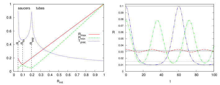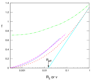
Right: $\mathcal{R}(t)$ plotted for three saucer orbits (equation 2 for $\mathcal{R}_{\mathrm{sep}}=0.1,\mathcal{R}_{z}=0.01$). Red dashed, green dashed-dotted and blue dash-double-dotted lines are for $\mathcal{H}=-0.048$ (close to the fixed-point orbit), $\mathcal{H}=-0.02$ and $\mathcal{H}=-0.001$ (close to separatrix). Thin solid lines show minimum and maximum possible values of $\mathcal{R}$ for given $\mathcal{R}_{z}$ (essentially $\mathcal{R}_{z}$ and $\mathcal{R}_{\mathrm{sep}}$), and dotted line shows $\mathcal{R}_{\mathrm{fix}}=\sqrt{\mathcal{R}_{\mathrm{sep}}\mathcal{R}_{z}}\approx 0.032$. Another dotted line shows the capture boundary at $\mathcal{R}_{\mathrm{lc}}=0.015$.

In what follows, it will be convenient to replace $\tilde{H}$ by $\mathcal{H}$, a linear combination of $\tilde{H}$ and $\mathcal{R}_{z}$:

$$\mathcal{H}(\mathcal{R},\omega) \equiv \frac{Q(1-\epsilon_{p}/3)-\tilde{H}-(Q-1)(1-\epsilon_{p}/3)\mathcal{R}_{z}}{(Q-1)(1-\epsilon_{p}/3)-\epsilon_{p}/2}=$$ (11a)

$$= (\mathcal{R}-\mathcal{R}_{z})\left(1-\frac{\mathcal{R}_{\mathrm{sep}}}{1-\mathcal{R}_{\mathrm{sep}}}\frac{1-\mathcal{R}}{\mathcal{R}}\sin^{2}\omega\right),$$

$$\mathcal{R}_{\mathrm{sep}} \equiv \frac{Q\epsilon_{p}}{(Q-1)(1-\epsilon_{p}/3)-\epsilon_{p}/2+Q\epsilon_{p}}.$$ (11b)

To obtain the solution, we express $\omega$ from (11) and substitute it into the first of equations (9):

$$\frac{d\mathcal{R}}{d\tau} = -k\,\sqrt{(\mathcal{R}_{1}-\mathcal{R})(\mathcal{R}-\mathcal{R}_{2})(\mathcal{R}-\mathcal{R}_{3})},$$ (12a)

$$k \equiv \frac{4Q\epsilon_{p}\sqrt{1-\mathcal{R}_{\mathrm{sep}}}}{\mathcal{R}_{\mathrm{sep}}}\approx 4(Q-1)\;\mbox{ for }\epsilon_{p}\ll 1,$$

$$\mathcal{R}_{1,2} \equiv \mathcal{R}_{\star}\pm\sqrt{\mathcal{R}_{\star}^{2}-\mathcal{R}_{\mathrm{sep}}\mathcal{R}_{z}},$$ (12b)

$$\mathcal{R}_{3} \equiv \mathcal{H}+\mathcal{R}_{z},$$

$$\mathcal{R}_{\star} \equiv \frac{1}{2}\left[\mathcal{R}_{\mathrm{sep}}(1+\mathcal{R}_{z})+(1-\mathcal{R}_{\mathrm{sep}})(\mathcal{H}+\mathcal{R}_{z})\right].$$

$${\mathcal{R}}_{\mathrm{max}} \equiv \mathcal{R}_{1},$$ (12c)

$${\mathcal{R}}_{\mathrm{min}} \equiv \mathrm{max}(\mathcal{R}_{2},\mathcal{R}_{3}),$$

$${\mathcal{R}}_{\mathrm{low}} \equiv \mathrm{min}(\mathcal{R}_{2},\mathcal{R}_{3}).$$

It is clear that $\mathcal{R}$ is allowed to oscillate between ${\mathcal{R}}_{\mathrm{min}}$ and ${\mathcal{R}}_{\mathrm{max}}$. We thus have two classes of orbit, depending on the relation between $\mathcal{R}_{2}$ and $\mathcal{R}_{3}$. If $\mathcal{R}_{3}\geq\mathcal{R}_{2}$, which occurs when $\mathcal{H}\geq 0$, the orbit is an ordinary short-axis tube (SAT); in the opposite case ($\mathcal{H}<0$) the orbit is a saucer, with $\mathcal{R}_{3}<\mathcal{R}_{2}$. (A similar class of orbits was described by Lees & Schwarzschild (1992) for a $\gamma=2$ scale-free potential; see Appendix D for more discussion). The main distinction is that for saucer orbits the angle $\omega$ librates around $\pi/2$, which means the apoapsis always lies above (or below) the $x-y$ plane; the orbit resembles a conical saucer with inner hole (e.g. Sambhus & Sridhar, 2000, Figure 7). For tubes, conversely, $\omega$ steadily decreases. Saucer orbits only exist in the oblate, not prolate case; the condition that the expression under the radical in (12b) is nonnegative requires that $\mathcal{R}_{z}\leq\mathcal{R}_{\mathrm{sep}}$, hence the label “separatrix”.

The solution to equation (12a) can be expressed exactly in terms of the elliptic cosine (e.g. Abramovitz & Stegun, 1972, Chapter 16; their parameter $m=k^{2}$, where $k$ is the elliptic modulus used as the second parameter in our notation):

$$\mathcal{R} = {\mathcal{R}}_{\mathrm{min}}+({\mathcal{R}}_{\mathrm{max}}-{\mathcal{R}}_{\mathrm{min}})\times$$

$$\times \mathrm{cn}^{2}\left(\frac{k\sqrt{{\mathcal{R}}_{\mathrm{max}}-{\mathcal{R}}_{\mathrm{low}}}}{2}\,\tau,\sqrt{\frac{{\mathcal{R}}_{\mathrm{max}}-{\mathcal{R}}_{\mathrm{min}}}{{\mathcal{R}}_{\mathrm{max}}-{\mathcal{R}}_{\mathrm{low}}}}\right).$$

We call the period of full oscillation in $\mathcal{R}$ the “precession time.” It is given by the complete elliptic integral:

$$T_{\mathrm{prec}}=\frac{2}{\pi}\frac{T_{\mathrm{M}}}{k\sqrt{{\mathcal{R}}_{\mathrm{max}}-{\mathcal{R}}_{\mathrm{low}}}}\,K\left(\sqrt{\frac{{\mathcal{R}}_{\mathrm{max}}-{\mathcal{R}}_{\mathrm{min}}}{{\mathcal{R}}_{\mathrm{max}}-{\mathcal{R}}_{\mathrm{low}}}}\right).$$ (14)

For orbits not too close to the separatrix, $K\approx\pi/2$.

It is also useful to write down expressions relating ${\mathcal{R}}_{\mathrm{min}}$ and ${\mathcal{R}}_{\mathrm{max}}$. For tube orbits,

$${\mathcal{R}}_{\mathrm{min}}={\mathcal{R}}_{\mathrm{max}}-\frac{\mathcal{R}_{\mathrm{sep}}}{1-\mathcal{R}_{\mathrm{sep}}}\frac{(1-{\mathcal{R}}_{\mathrm{max}})({\mathcal{R}}_{\mathrm{max}}-\mathcal{R}_{z})}{{\mathcal{R}}_{\mathrm{max}}}.$$ (15)

It is clear that if $\epsilon_{p}\ll 1$ and $\mathcal{R}_{\mathrm{sep}}\ll\mathcal{R}\lesssim 1$, these two values are quite close to each other, justifying the practice of approximating the third integral as $L^{2}$.

For saucer orbits, the relation is simpler:

$${\mathcal{R}}_{\mathrm{min}}{\mathcal{R}}_{\mathrm{max}}=\mathcal{R}_{\mathrm{sep}}\mathcal{R}_{z}.$$ (16)

In particular, the condition ${\mathcal{R}}_{\mathrm{min}}={\mathcal{R}}_{\mathrm{max}}$ gives the fixed-point orbit, for which $\omega=\pi/2$ always. Figure 1 shows the properties of a series of orbits with the same $\mathcal{R}_{z}<\mathcal{R}_{\mathrm{sep}}$ which start with $\omega=\pi/2$ and with different initial angular momenta $\mathcal{R}_{\mathrm{init}}$ (left panel), and the time evolution of $\mathcal{R}$ for several saucer orbits with different values of $\mathcal{H}$ (right panel).

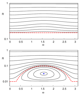
Equation (11) can be inverted to express $\mathcal{R}$ as a function of $\omega$ (Figure 2), which is more convenient for the averaging procedure in the next section:

$$\mathcal{R}(\omega) = \frac{\mathcal{R}_{a}\pm\sqrt{\mathcal{R}_{a}^{2}-4\mathcal{R}_{z}\mathcal{R}_{b}(1+\mathcal{R}_{b})}}{2(1+\mathcal{R}_{b})}\;,$$ (17a)

$$\mathcal{R}_{b} \equiv \frac{\mathcal{R}_{\mathrm{sep}}\sin^{2}\omega}{1-\mathcal{R}_{\mathrm{sep}}}\;,\;\;\mathcal{R}_{a}\equiv\mathcal{H}+\mathcal{R}_{z}+\mathcal{R}_{b}(1+\mathcal{R}_{z}).$$

For tubes only the upper root has physical meaning, while for saucers both roots are valid as long as $\sin^{2}\omega$ is greater than the following threshold:

$$\begin{array}[]{l}\displaystyle\sin^{2}\omega_{\mathrm{min}}\equiv\frac{1-\mathcal{R}_{\mathrm{sep}}}{\mathcal{R}_{\mathrm{sep}}}\;\times\\ \displaystyle\frac{\mathcal{R}_{z}(1-\mathcal{H}-\mathcal{R}_{z})-\mathcal{H}+2\sqrt{-\mathcal{H}\mathcal{R}_{z}(1-\mathcal{H}-\mathcal{R}_{z})}}{(1-\mathcal{R}_{z})^{2}}.\end{array}$$ (18)

This condition arises from nonnegativity of the expression under the radical in (17a). Therefore, in a time $T_{\mathrm{prec}}$, $\omega$ varies by $\pi$ for tube orbits and by an amount $\leq\pi$ for saucers.

Figure 2.— $\mathcal{R}(w)$ (equation 17) for sets of orbits with the same $\mathcal{R}_{z}$ and different $\mathcal{H}$. Top panel: $\mathcal{R}_{\mathrm{sep}}=0.1,\mathcal{R}_{z}=0.15$, which has only tube orbits; bottom panel: $\mathcal{R}_{\mathrm{sep}}=0.1,\mathcal{R}_{z}=0.01$, which has saucer orbits appearing as cycles in the lower part of the plot. The fixed-point orbit is marked by the cross. In the upper panel, the dashed (red) line is at $\mathcal{R}=\mathcal{R}_{z}$ and in the lower panel it marks the separatrix.

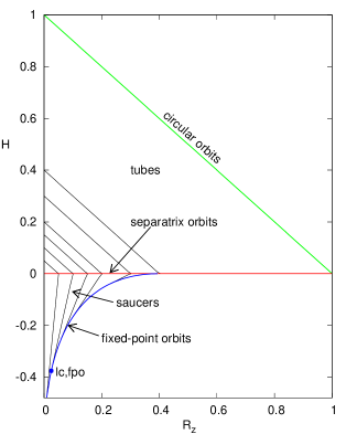
Finally, we outline the complete phase space in ($\mathcal{H},\mathcal{R}_{z}$) coordinates (Figure 3). The boundary between tubes and saucers is $\mathcal{H}=0$, and the other important boundaries are

$$\mathcal{H}=1-\mathcal{R}_{z},$$ (19a)

the location of circular orbits ($$\mathcal{R}=1$$), and

$$\mathcal{H}=-\frac{\mathcal{R}_{\mathrm{sep}}}{1-\mathcal{R}_{\mathrm{sep}}}\left(1-\sqrt{\frac{\mathcal{R}_{z}}{\mathcal{R}_{\mathrm{sep}}}}\right)^{2}$$ (19b)

is the line of fixed-point saucer orbits, for which $$\omega_{\mathrm{min}}=\pi/2$$.

A star is captured if it passes near periapsis while having $\mathcal{R}<\mathcal{R}_{\mathrm{lc}}$, where $\mathcal{R}_{\mathrm{lc}}\equiv L_{\mathrm{lc}}^{2}/I^{2}\approx 2r_{\mathrm{lc}}/a$ is the absorption boundary ($r_{\mathrm{lc}}$ is the distance to SBH at which a star is either tidally disrupted or captured directly, and $a$ is the semimajor axis). In the axisymmetric system, this condition corresponds to ${\mathcal{R}}_{\mathrm{min}}<\mathcal{R}_{\mathrm{lc}}$, although not every star satisfying this condition is immediately lost (see §4). The lines of constant ${\mathcal{R}}_{\mathrm{min}}=\mathcal{R}_{\mathrm{lc}}$, which mark the SBH capture boundary, are straight lines satisfying

$$\mathcal{H}=\left\{\begin{array}[]{ll}\mathcal{R}_{\mathrm{lc}}-\mathcal{R}_{z}&\mbox{for tubes}\\ -\frac{(\mathcal{R}_{\mathrm{lc}}-\mathcal{R}_{z})(\mathcal{R}_{\mathrm{sep}}-\mathcal{R}_{\mathrm{lc}})}{(1-\mathcal{R}_{\mathrm{sep}})\mathcal{R}_{\mathrm{lc}}}&\mbox{for saucers.}\end{array}\right.$$ (20)

This boundary in the saucer region touches the fixed-point orbit curve (19b) at

$$\mathcal{H}_{\mathrm{lc,FPO}}=-\frac{(\mathcal{R}_{\mathrm{sep}}-\mathcal{R}_{\mathrm{lc}})^{2}}{\mathcal{R}_{\mathrm{sep}}(1-\mathcal{R}_{\mathrm{sep}})}\;,\quad\mathcal{R}_{z,\mathrm{lc,FPO}}=\frac{\mathcal{R}_{\mathrm{lc}}^{2}}{\mathcal{R}_{\mathrm{sep}}}$$ (21)

In what follows, we will often assume that $\mathcal{R}_{\mathrm{sep}}\ll 1$ (or at least not too large), equivalent to assuming that the nuclear flattening is modest. An isotropic distribution of stars in velocity space corresponds to a distribution function which doesn’t depend on $\{L,L_{z},\omega,\Omega\}$; in these canonical action-angle variables, the phase-space volume element is constant and we can compute the proportion of phase space occupied by saucer orbits by sampling initial conditions from a uniform distribution in these variables and recording the fraction of cases for which $\mathcal{H}<0$. For small $\mathcal{R}_{\mathrm{sep}}$, the fraction of saucer orbits turns out to be approximately $0.4\mathcal{R}_{\mathrm{sep}}$, i.e. proportional to the degree of flattening measured by $\epsilon_{p}$ (1d, 11b).

Figure 3.— Phase space in ($\mathcal{R}_{z},\mathcal{H}$) coordinates, for $\mathcal{R}_{\mathrm{sep}}=0.4$. The region $0<\mathcal{H}<1-\mathcal{R}_{z}$ is occupied by tube orbits, and the bottom left corner by saucer orbits; the lower boundary (blue) corresponds to fixed-point saucer orbits (equation 19b). Shown in black are lines of constant minimum angular momentum (equation 20) for $\mathcal{R}_{\mathrm{lc}}=(0.05,0.1,0.15,0.2,0.3,0.4)$. A dot on the intersection of the fixed-point orbit curve and the line of $\mathcal{R}_{\mathrm{lc}}=0.1$ has coordinates given by (21).

3. Fokker-Planck equation

We begin by outlining the general method for deriving the covariant Fokker-Planck equation in arbitrary coordinates (Rosenbluth et al., 1957).

The local (position-dependent) Fokker-Planck equation can be expressed in terms of generalized position- and velocity-space coordinates $(x^{\alpha},J^{\alpha})$, $\alpha=\{1,2,3\}$ as

$$\frac{\partial[\mathcal{G}f(x^{\alpha},J^{\alpha},t)]}{\partial t} = -\frac{\partial}{\partial J^{\alpha}}(\langle\Delta J^{\alpha}\rangle\mathcal{G}f)\;+$$

$$+ \frac{1}{2}\frac{\partial^{2}}{\partial J^{\alpha}\partial J^{\beta}}(\langle\Delta J^{\alpha}\Delta J^{\beta}\rangle\mathcal{G}f)$$

(Merritt, 2013, equation (5.121)). The position and velocity coordinates need not be related to each other in any particular way (e.g. they need not be canonically conjugate): for instance, one can adopt the integrals of motion as the velocity-space coordinates. In equation (3), coefficients in angled brackets represent average and mean square changes of the corresponding velocity variables per unit time. Equation (3) is valid under the assumptions of (i) local encounters that change only the velocity but not the position of a star; (ii) weak interactions, which allows the collision term to be expanded in powers of $\Delta J^{\alpha}$ up to second order. Later in this section we will use the orbit-averaged form of this equation, which additionally requires that the significant changes in $J^{\alpha}$ occur on a time scale much longer than the orbital period.

The quantity $\mathcal{G}\equiv a^{1/2}$ is the density of states, with $a$ the determinant of the velocity-space metric tensor $a_{\alpha\beta}$, so that the squared distance between two points whose coordinates differ by $\Delta\boldsymbol{J}$ is given by $ds^{2}=a_{\alpha\beta}\Delta J^{\alpha}\Delta J^{\beta}$, and the number of stars in the phase-space volume $d^{3}Jd^{3}x$ is $dN=\mathcal{G}fd^{3}Jd^{3}x$ (generalization to an arbitrary, non-trivial metric in coordinate space is straightforward). Under a change of coordinates $J^{\alpha}\to\tilde{J}^{\mu}$, the coefficients in equation (3) transform as

$$\langle\Delta\tilde{J}^{\mu}\rangle = \langle\Delta J^{\alpha}\rangle\frac{\partial\tilde{J}^{\mu}}{\partial J^{\alpha}}+\frac{1}{2}\langle\Delta J^{\alpha}\Delta J^{\beta}\rangle\frac{\partial^{2}\tilde{J}^{\mu}}{\partial J^{\alpha}\partial J^{\beta}},$$

$$\langle\Delta\tilde{J}^{\mu}\Delta\tilde{J}^{\nu}\rangle = \langle\Delta J^{\alpha}\Delta J^{\beta}\rangle\frac{\partial\tilde{J}^{\mu}}{\partial J^{\alpha}}\frac{d\tilde{J}^{\nu}}{\partial J^{\beta}}$$ (23b)

(Merritt, 2013, equation (5.120)) and

$$\tilde{\mathcal{G}}=\mathcal{G}\,\det\left\|\frac{\partial J^{\alpha}}{\partial\tilde{J}^{\mu}}\right\|.$$ (24)

To compute the diffusion coefficients $\langle\Delta J^{\alpha}\rangle$, $\langle\Delta J^{\alpha}\Delta J^{\beta}\rangle$, one needs to know the distribution function describing the field stars. Here we assume that the test and field stars are drawn from the same $f$, but as is often done, we replace the exact $f$ by an approximation when computing the diffusion coefficients. Namely, we neglect changes in the diffusion coefficients caused by the evolution, and compute them assuming a field star distribution of the form $f(\mathcal{E})$, where $\mathcal{E}\equiv-E$ is the binding energy per unit mass. In other words, we neglect the anisotropy of the field star distribution. Consistency with the (spherically-symmetric part of the) mass model (1a) requires that

$$f(\mathcal{E})=f_{0}\mathcal{E}^{\gamma-3/2}\,,\;\;f_{0}=\frac{\rho_{0}}{m_{\star}}\left(\frac{GM_{\bullet}}{r_{0}}\right)^{-\gamma}\!\!\!\!\frac{\Gamma(\gamma+1)}{(2\pi)^{3/2}\,\Gamma(\gamma-\frac{1}{2})},$$ (25)

The assumption of isotropy in the field-star distribution is obviously inconsistent with the density model being flattened; however, for a small degree of flattening it is a reasonable approximation. The flattening may be due to streaming motions, to an elongated velocity ellipsoid or to both; deviations from isotropy due to nuclear flattening are of order $\epsilon_{p}\ll 1$.

For an isotropic field-star population, the diffusion coefficients expressed in terms of $\{v_{\|},v_{\bot}\}$ are well known (e.g. Merritt, 2013, equations 5.23, 5.55) and may be transformed to any other coordinates using (23). We first adopt the velocity-space variables $J^{\alpha}=\{\mathcal{E},\mathcal{R},\mathcal{R}_{z}\}$, then later replace $\mathcal{R}$ by $\mathcal{H}$ which is a true integral of the motion. The expressions for the local diffusion coefficients in these coordinates are given in Appendix E, equations (E1).

The orbit-averaged Fokker-Planck equation is obtained by (i) selecting integrals of motion as the velocity-space coordinates; (ii) integrating the local Fokker-Planck equation over the phase-space volume filled by an orbit, assuming that $f(x^{\alpha},J^{\alpha})$ is a constant in this region (Jeans’s theorem); (iii) using the Leibnitz-Reynolds transport theorem to exchange the order of integration and differentiation. The result is

$$\frac{\partial[\mathcal{G}_{\mathrm{av}}f(J^{\alpha},t)]}{\partial t} = -\frac{\partial}{\partial J^{\alpha}}(\langle\Delta J^{\alpha}\rangle_{\mathrm{av}}\mathcal{G}_{\mathrm{av}}f)\;+$$

$$+ \frac{1}{2}\frac{\partial^{2}}{\partial J^{\alpha}\partial J^{\beta}}(\langle\Delta J^{\alpha}\Delta J^{\beta}\rangle_{\mathrm{av}}\mathcal{G}_{\mathrm{av}}f)$$

(Merritt, 2013, equation (5.153)), which has the same form as the local equation (3), but now $f$ is understood to be a function of the $J^{\alpha}$ and of $t$ only, and the diffusion coefficients are averaged according to

$$\langle X\rangle_{\mathrm{av}}\mathcal{G}_{\mathrm{av}} \equiv \int_{\mathrm{orbit}}\langle X\rangle\,\mathcal{G}\;d^{3}x.$$ (27)

Setting $X=1$ in this expression gives the “density of states” $\mathcal{G}_{\mathrm{av}}$, which relates $f$ to the number of stars in a velocity space volume element $d^{3}J$: $dN=f\,\mathcal{G}_{\mathrm{av}}d^{3}J$.

In the spherically-symmetric case, orbit averaging reduces to a one-dimensional integration with respect to radius, $\int_{r_{-}}^{r_{+}}Xdr/v_{r}$, where $r_{-}$ and $r_{+}$ are peri- and apoapsis radii for a given $E$ and $L$; in other words, averaging reduces to weighting $X$ in proportion to the time an orbit spends near $r$. In the axisymmetric case, what is traditionally done (Goodman, 1983; Einsel & Spurzem, 1999) is to assume that the orbit fills the configuration-space region defined by the condition $E-\Phi(R,z)-L_{z}^{2}/(2R^{2})\geq 0$ where ($R,z$) are cylindrical coordinates; in other words, existence of a third integral is ignored. Then the average turns out to be proportional simply to $\int\!\!\int X\,dR\,dz$, the integral being taken over this region.

In our case, the distinction between saucer and tube orbits is critical for the loss-cone problem and we do not want to mix orbits having different values of the third integral. We must perform the averaging taking into account the shapes of the orbits as described in the previous section. This is most easily done by adopting Delaunay angular variables ($w,\omega,\Omega$) as configuration-space coordinates $x^{\alpha}$. If the corresponding actions ($I,L,L_{z}$) were taken as velocity-space coordinates $J^{\alpha}$, the Jacobian $\mathcal{G}$ of this coordinate system would be unity; but since we are using a different set of $J^{\alpha}$, $\mathcal{G}$ is determined by equation (24) for the coordinates of choice.

We split this transformation, and the averaging procedure, into two steps. Initially we adopt ($\mathcal{E},\mathcal{R},\mathcal{R}_{z}$) as generalized velocities $J^{\alpha}$ and carry out the averaging over the radial phase angle (mean anomaly) $w$, obtaining the coefficients for the spherical problem. Since these do not depend on $\omega$ or $\Omega$, averaging over these two angles means simply multiplying by $(2\pi)^{2}$:

$$\langle X\rangle_{\mathrm{sph}}\mathcal{G}_{\mathrm{sph}}\equiv 4\pi^{2}\int_{0}^{2\pi}dw\,\langle X\rangle\,\det\left\|\frac{\partial\{I,L,L_{z}\}}{\partial\{\mathcal{E},\mathcal{R},\mathcal{R}_{z}\}}\right\|.$$

Here all coefficients, including the Jacobian (explicitly written as a determinant), are understood to be functions of ($\mathcal{E},\mathcal{R},\mathcal{R}_{z}$). In the case of a Keplerian potential $\Phi(r)=-GM_{\bullet}/r$ (i.e. neglecting the contribution of the stars), and assuming a power-law density profile for the stars with index $\gamma=3/2$, the field star distribution function (in our isotropic approximation) is a constant $f_{0}$ (equation 25), and the diffusion coefficients can be expressed in terms of elementary functions as

$$\langle\Delta\mathcal{E}\rangle_{\mathrm{sph}} = \mathcal{A}\,\mathcal{E}\,\left(\frac{2}{3}\frac{m}{m_{\star}}-1\right),$$ (29a)

$$\langle\Delta\mathcal{R}\rangle_{\mathrm{sph}} = \mathcal{A}\,\frac{29-66\mathcal{R}}{15},$$ (29b)

$$\langle\Delta\mathcal{R}_{z}\rangle_{\mathrm{sph}} = \langle\Delta\mathcal{R}\rangle_{\mathrm{sph}}\,\frac{\mathcal{R}_{z}}{\mathcal{R}}+\frac{\mathcal{A}}{30\mathcal{R}}\big{\{}9\mathcal{R}(\mathcal{R}-3\mathcal{R}_{z})$$ (29c)

$$+ 29(1-\mathcal{R})[(\mathcal{R}-\mathcal{R}_{z})\cos^{2}\omega-\mathcal{R}_{z}]\big{\}}\qquad\phantom{.}$$

$$\langle(\Delta\mathcal{E})^{2}\rangle_{\mathrm{sph}} = \mathcal{A}\,\mathcal{E}^{2}\;\frac{32-4\sqrt{\mathcal{R}}}{15\sqrt{\mathcal{R}}},$$ (29d)

$$\langle(\Delta\mathcal{R})^{2}\rangle_{\mathrm{sph}} = \mathcal{A}\,\mathcal{R}\,\frac{58+32\sqrt{\mathcal{R}}-90\mathcal{R}}{15},$$ (29e)

$$\langle(\Delta\mathcal{R}_{z})^{2}\rangle_{\mathrm{sph}} = \langle(\Delta\mathcal{R})^{2}\rangle_{\mathrm{sph}}\left(\frac{\mathcal{R}_{z}}{\mathcal{R}}\right)^{2}+\frac{2\mathcal{A}}{15}(\mathcal{R}-\mathcal{R}_{z})$$ (29f)

$$\times \frac{\mathcal{R}_{z}}{\mathcal{R}}\big{[}9\mathcal{R}+29(1-\mathcal{R})\cos^{2}\omega\big{]},$$

$$\langle\Delta\mathcal{E}\Delta\mathcal{R}\rangle_{\mathrm{sph}} = \mathcal{A}\,\mathcal{E}\,\frac{32\sqrt{\mathcal{R}}(1-\sqrt{\mathcal{R}})}{15},$$ (29g)

$$\langle\Delta\mathcal{E}\Delta\mathcal{R}_{z}\rangle_{\mathrm{sph}} = \langle\Delta\mathcal{E}\Delta\mathcal{R}\rangle_{\mathrm{sph}}\frac{\mathcal{R}_{z}}{\mathcal{R}},$$ (29h)

$$\langle\Delta\mathcal{R}\Delta\mathcal{R}_{z}\rangle_{\mathrm{sph}} = \langle\Delta\mathcal{R}^{2}\rangle_{\mathrm{sph}}\frac{\mathcal{R}_{z}}{\mathcal{R}}$$ (29i)

where

$$\mathcal{A}\equiv 16\pi^{2}G^{2}m_{\star}^{2}\ln\Lambda\,f_{0}.$$ (30)

Here $m_{\star}$ is the mass of a field star (scatterer) and $m$ is the mass of a test star (whose evolution is described by the Fokker-Planck equation). We set $m_{\star}=m$ in what follows.

The density of states $\mathcal{G}_{\mathrm{sph}}$ is split into two factors:

$$\mathcal{G}_{\mathrm{sph}}=\frac{\mathcal{G}_{\mathcal{E}}}{2\sqrt{\mathcal{R}\mathcal{R}_{z}}}\;,\quad\mathcal{G}_{\mathcal{E}}\equiv\frac{\sqrt{2}\,\pi^{3}\,(GM_{\bullet})^{3}}{\mathcal{E}^{5/2}}$$ (31)

so that $\int_{0}^{1}d\mathcal{R}\int_{0}^{\mathcal{R}}d\mathcal{R}_{z}\,\mathcal{G}_{\mathrm{sph}}=\mathcal{G}_{\mathcal{E}}$ is the phase space volume element that transforms $f$ to the number density of stars $\mathcal{N}$ in the spherical geometry:

$$\mathcal{N}(\mathcal{E},\mathcal{R})\,d\mathcal{E}d\mathcal{R}=\mathcal{G}_{\mathcal{E}}(\mathcal{E})\,f(\mathcal{E},\mathcal{R})\,d\mathcal{E}d\mathcal{R}.$$ (32)

These coefficients are based on the usual approximation of uncorrelated two-body encounters. The effect of resonant relaxation (Rauch & Tremaine, 1996) would be to enhance the diffusion coefficients for $\mathcal{R}$ and $\mathcal{R}_{z}$; we defer a discussion of this until §8.

Finally, the diffusion coefficients are expressed in terms of $\{\mathcal{E},\mathcal{H},\mathcal{R}_{z}\}$ by substituting $\mathcal{H}(\mathcal{R},\mathcal{R}_{z},\omega)$ from equation (11), transforming the above coefficients under this substitution according to equation (23), and averaging over the argument of periastron (i.e. the precession phase) $\omega$:

$$\langle X\rangle_{\mathrm{av}}\mathcal{G}_{\mathrm{av}}=\frac{1}{\pi}\int_{\omega_{\mathrm{min}}}^{\pi-\omega_{\mathrm{min}}}d\omega\,\langle\tilde{X}\rangle_{\mathrm{sph}}\,\frac{\partial\mathcal{R}}{\partial\mathcal{H}}\,\mathcal{G}_{\mathrm{sph}}.$$ (33)

We have explicitly written the Jacobian of transformation (24), and the coefficients with tildes are transformed from $\langle X\rangle_{\mathrm{sph}}$ using (23). This is possible because the last transformation does not depend on $w$ or $\Omega$. The limits of integration in (33) are between 0 and $\pi$ for tubes and between $\omega_{\mathrm{min}}$ and $\pi-\omega_{\mathrm{min}}$ for saucers (equation 18). From here on, we omit the subscript for the averaged coefficients.

The averaging must be done numerically, however, we can derive asymptotic expressions for the diffusion coefficients in the large- and small-$\mathcal{R}$ regimes. In the former case, when $\mathcal{R}\gg\mathcal{R}_{\mathrm{sep}}$, $\mathcal{R}\approx\mathrm{const}=\mathcal{H}+\mathcal{R}_{z}$, so we trivially get $\langle\Delta\mathcal{H}^{2}\rangle=\langle(\Delta\mathcal{R})^{2}\rangle-2\langle\Delta\mathcal{R}\Delta\mathcal{R}_{z}\rangle+\langle(\Delta\mathcal{R}_{z})^{2}\rangle$, $\langle\Delta\mathcal{H}\Delta\mathcal{R}_{z}\rangle=\langle(\Delta\mathcal{R})^{2}\rangle-\langle\Delta\mathcal{R}\Delta\mathcal{R}_{z}\rangle$.

In the limit of small $\mathcal{R}$, i.e. close to the capture boundary, the asymptotic behavior of the coefficients is different in the tube and saucer regions. In the case of tube orbits with $\mathcal{H}+\mathcal{R}_{z}\ll\mathcal{R}_{\mathrm{sep}}$, the asymptotic expressions are

$$\langle\Delta\mathcal{H}^{2}\rangle\approx\mathcal{A}\frac{58}{15}\frac{\mathcal{R}_{\mathrm{sep}}}{b}\;,\quad\mathcal{G}_{\mathrm{av}}\approx\frac{2b}{\pi}\frac{\mathcal{G}_{\mathcal{E}}}{2\sqrt{\mathcal{R}_{\mathrm{sep}}\mathcal{R}_{z}}}\;,$$ (34)

where $b\equiv 2\ln 2-\frac{1}{2}\ln(\mathcal{R}_{z}/\mathcal{R}_{\mathrm{sep}})$; the other two diffusion coefficients are smaller that $\langle\Delta\mathcal{H}^{2}\rangle$ by a factor $\sim\mathcal{R}_{z}/\mathcal{R}_{\mathrm{sep}}$. For saucer orbits with $\mathcal{R}_{z}\ll\mathcal{R}_{\mathrm{sep}}$ and not too close to either the separatrix or the fixed-point orbit, the asymptotic expressions for the diffusion coefficients are estimated to within $\mathcal{O}(1)$ as

$$\langle(\Delta\mathcal{R}_{z})^{2}\rangle\approx 2\mathcal{A}\left(1+\frac{\mathcal{H}}{\mathcal{R}_{\mathrm{sep}}}\right)\,\mathcal{R}_{z}\;,\quad\langle\Delta\mathcal{H}\Delta\mathcal{R}_{z}\rangle\approx 4\mathcal{A}\mathcal{R}_{z}\;,$$

$$\langle\Delta\mathcal{H}^{2}\rangle\approx\langle\Delta\mathcal{H}^{2}\rangle\,\frac{\mathcal{R}_{\mathrm{sep}}}{\mathcal{R}_{z}}\;,\quad\mathcal{G}_{\mathrm{av}}\approx\frac{\mathcal{G}_{\mathcal{E}}}{\sqrt{2\mathcal{R}_{\mathrm{sep}}\mathcal{R}_{z}}}.\\$$ (35)

Finally, it is convenient to cast the orbit-averaged Fokker-Planck equation (3) into flux-conservative form:

$$\frac{\partial(\mathcal{G}_{\mathrm{av}}f)}{\partial t}=-\frac{\partial F^{\alpha}}{\partial J^{\alpha}}\;,\quad F^{\alpha}\equiv-\mathcal{D}^{\alpha}f-\mathcal{D}^{\alpha\beta}\frac{\partial f}{\partial J^{\beta}}.$$ (36)

The drift and diffusion coefficients are

$$\mathcal{D}^{\alpha} = -\mathcal{G}_{\mathrm{av}}\langle\Delta J^{\alpha}\rangle+\frac{\partial}{\partial J^{\beta}}\left(\frac{1}{2}\mathcal{G}_{\mathrm{av}}\langle\Delta J^{\alpha}\Delta J^{\beta}\rangle\right),\quad\phantom{,}$$ (37a)

$$\mathcal{D}^{\alpha\beta} = \frac{1}{2}\mathcal{G}_{\mathrm{av}}\langle\Delta J^{\alpha}\Delta J^{\beta}\rangle.$$ (37b)

This form is convenient from both from a computational and a physical point of view, since (i) it manifestly conserves the total number of stars, and (ii) drift coefficients $\mathcal{D}_{\mathcal{R}}$ and $\mathcal{D}_{\mathcal{R}_{z}}$ must be zero, which may be demonstrated explicitly, or inferred from the natural requirement that (in the absence of capture) collisions tend to isotropize $f$, i.e. in the steady state $f$ should not depend on $\mathcal{R}$ or $\mathcal{R}_{z}$.

4. Boundary conditions

As is well known, the steady-state loss rate in the spherical geometry can only be inferred from the orbit-averaged Fokker-Planck equation if a certain condition is satisfied: the change in angular momentum over one radial period due to encounters must be small for orbits near the loss cone. Far enough from the SBH, this condition is violated (the “pinhole” or “full-loss-cone” regime) and the orbit-averaged approximation is not valid. This problem is dealt with by returning to the local $(r,v)$ Fokker-Planck equation and allowing the phase-space density to vary along orbits, from zero at the edge of the capture sphere to some finite value at apoapsis (Cohn & Kulsrud, 1978). The result is a boundary condition for the Fokker-Planck equation that specifies the value and slope of $f(\mathcal{R})$ at $\mathcal{R}=\mathcal{R}_{\mathrm{lc}}$ in terms of its average value at the (fixed) energy $\mathcal{E}$.

No such exact analysis has ever been carried out in nonspherical (axisymmetric, triaxial) geometries, nor will we do so here. Instead we will be satisfied with a more heuristic derivation of the relation between $f$ and $\mathcal{F}$ at the loss cone boundary. Our analysis will be similar in spirit to that of Magorrian & Tremaine (1999), but, as we will see, with some important differences.

4.1. The spherical problem

We begin by reviewing the boundary conditions in the spherical geometry. The evolution equation in terms of $\mathcal{E}$ and $\mathcal{R}$ can be derived by integrating equation (36) over $\mathcal{R}_{z}$ from 0 to $\mathcal{R}$. We introduce two, two-dimensional quantities: the number density of stars,

$$\mathcal{N}(\mathcal{E},\mathcal{R})\,d\mathcal{E}d\mathcal{R} \equiv \int_{0}^{\mathcal{R}}\!\!d\mathcal{R}_{z}\,\mathcal{G}_{\mathrm{sph}}(\mathcal{E},\mathcal{R},\mathcal{R}_{z})\,f(\mathcal{E},\mathcal{R},\mathcal{R}_{z})\,d\mathcal{E}d\mathcal{R}$$ (38)

$$= 4\pi^{2}T_{\mathrm{rad}}(\mathcal{E})L_{\mathrm{circ}}^{2}(\mathcal{E})\,f(\mathcal{E},\mathcal{R})\,d\mathcal{E}d\mathcal{R}$$

$$= \mathcal{G}_{\mathcal{E}}(\mathcal{E})\,f(\mathcal{E},\mathcal{R})\,d\mathcal{E}d\mathcal{R},$$

and the flux per unit energy in the $\mathcal{R}$-direction:

$$\mathcal{F}_{\mathcal{R}}(\mathcal{E},\mathcal{R})\,d\mathcal{E} = -\int_{0}^{\mathcal{R}}d\mathcal{R}_{z}\,\mathcal{G}_{\mathrm{sph}}\,\frac{\langle(\Delta\mathcal{R})^{2}\rangle}{2}\,\frac{\partial f}{\partial\mathcal{R}}\,d\mathcal{E}$$ (39)

$$= \frac{\langle(\Delta\mathcal{R})^{2}\rangle}{2}\frac{\partial\mathcal{N}(\mathcal{E},\mathcal{R})}{\partial\mathcal{R}}\,d\mathcal{E}.$$

The relation between $\mathcal{F}_{\mathcal{R}}$ and the fluxes appearing in equation (36) is that the former is the integral, over the entire loss cone boundary, of the component of $F^{\alpha}$ normal to that boundary, in the subspace $\mathcal{E}=\mathrm{const}$. In the spherical case, the capture boundary in the $\mathcal{R}-\mathcal{R}_{z}$ plane is defined by $\mathcal{R}=\mathcal{R}_{\mathrm{lc}}$, and so $\mathcal{F}_{\mathcal{R}}=\int_{0}^{\mathcal{R}}d\mathcal{R}_{z}\,F^{\mathcal{R}}$.

As emphasized by Frank & Rees (1976), in the spherical geometry, changes in angular momentum are expected to dominate the capture rate. Setting $\mathcal{E}=$ constant, we consider one-dimensional diffusion in $\mathcal{R}$, which obeys

$$\frac{\partial\mathcal{N}(\mathcal{R},t)}{\partial t}=-\frac{\partial\mathcal{F}_{\mathcal{R}}}{\partial\mathcal{R}}$$

$$=-\frac{\partial}{\partial\mathcal{R}}\left(\mathcal{N}\langle\Delta\mathcal{R}\rangle\right)+\frac{1}{2}\frac{\partial^{2}\mathcal{N}}{\partial\mathcal{R}^{2}}\left(\mathcal{N}\langle(\Delta\mathcal{R})^{2}\rangle\right)$$

$$\approx\frac{1}{2}\frac{\partial}{\partial\mathcal{R}}\left(\langle(\Delta\mathcal{R})^{2}\rangle\frac{\partial\mathcal{N}}{\partial\mathcal{R}}\right).$$ (40)

The final expression uses the result that for small $\mathcal{R}$, $\langle\Delta\mathcal{R}\rangle=\frac{1}{2}(\partial/\partial\mathcal{R})\langle(\Delta\mathcal{R})^{2}\rangle$. Also in this limit, $\langle(\Delta\mathcal{R})^{2}\rangle\propto\mathcal{R}$, and we can write

$$\mathcal{D}(\mathcal{E})\equiv\lim_{\mathcal{R}\to 0}\frac{\langle(\Delta\mathcal{R})^{2}\rangle}{2\mathcal{R}},$$ (41)

an inverse, orbit-averaged relaxation time.

If we adopt the approximation $\langle(\Delta\mathcal{R})^{2}\rangle/2=\mathcal{D}\mathcal{R}$ over the entire range of $\mathcal{R}$, then equation (40) is mathemathically equivalent to the heat conduction equation in a circular domain (Ozisik, 1993). The steady-state solution is $\mathcal{N}\propto\ln R+\mathrm{const}$. The natural boundary condition at $\mathcal{R}=1$ is $\mathcal{F}_{\mathcal{R}}=0$, which in this approximation translates to $\partial\mathcal{N}/\partial\mathcal{R}=0$ (in the more exact treatment, $\langle(\Delta\mathcal{R})^{2}\rangle$ itself tends to zero at $\mathcal{R}=1$). The boundary at $\mathcal{R}=\mathcal{R}_{\mathrm{lc}}$ is responsible for capture, however, simply setting $\mathcal{N}(\mathcal{R}_{\mathrm{lc}})=0$ is not always appropriate. As discussed by Lightman & Shapiro (1977), there are two regimes characterizing the behavior of $\mathcal{N}$ near loss cone boundary, depending on the ratio $q$ between the radial period and the time to random-walk out of the loss cone (that is, to change $\mathcal{R}$ by order of $\mathcal{R}_{\mathrm{lc}}$):

$$q(\mathcal{E})\equiv\frac{T_{\mathrm{rad}}}{T_{\mathrm{rw}}}\;,\quad T_{\mathrm{rw}}\equiv\frac{\mathcal{R}_{\mathrm{lc}}^{2}}{\langle(\Delta\mathcal{R})^{2}\rangle/2}=\frac{\mathcal{R}_{\mathrm{lc}}}{\mathcal{D}}.$$ (42)

The case $q\ll 1$ is the “empty loss cone” regime, since a star scattered into the region $\mathcal{R}\leq\mathcal{R}_{\mathrm{lc}}$ is swallowed much faster than encounters can scatter it back out. The opposite situation, $q\gg 1$, is the “full-loss-cone” regime, because diffusion is so rapid that even capture of stars (near periapsis) does not substantially diminish the population of loss cone orbits away from periapsis.

It turns out that much of the flux into the SBH comes from stars at energies where $q\approx 1$, so the behavior of the solution at the transition between the two regimes is important. Let $\mathcal{N}_{\mathrm{lc}}\equiv\mathcal{N}(\mathcal{R}_{\mathrm{lc}})$, and define $\mathcal{F}_{\mathrm{lc}}=-\mathcal{F}_{\mathcal{R}}(\mathcal{R}_{\mathrm{lc}})$, the flux through the boundary (i.e. the number of stars captured per unit time per unit energy). In a steady state, equation (40) implies that $\mathcal{F}_{\mathcal{R}}$ is independent of $\mathcal{R}$ near $\mathcal{R}_{\mathrm{lc}}$. We can express the inner boundary condition in a general way as

$$\mathcal{F}_{\mathrm{lc}}=\alpha^{-1}\mathcal{N}_{\mathrm{lc}}\mathcal{D}$$ (43)

where all quantities are understood to be functions of $\mathcal{E}$, or equivalently of $q(\mathcal{E})$. After usinq equations (38) and (39) to express $\mathcal{N}$ and $\mathcal{F}_{\mathcal{R}}$ in terms of $f$ and $\partial f/\partial\mathcal{R}$, equation (43) is seen to be a boundary condition of the Robin type (linear combination of function and its derivative) (Eriksson et al., 1996). The dimensionless coefficient $\alpha$ can be derived by returning to the local (non-orbit-averaged) Fokker-Planck equation and determining how $f$ varies with radial phase assuming $f=0$ at periapsis (Baldwin, Cordey & Watson, 1972). Cohn & Kulsrud (1978) produced a numerical solution in the spherical geometry and proposed the approximation $\alpha=0.186q+0.824\sqrt{q}$ for $q\leq 1$ and $\alpha=q$ for $q\geq 1$. An exact solution exists to the same set of equations solved by Cohn & Kulsrud:

$$\alpha(q)=\frac{q}{\xi(q)},\ \ \xi(q)=1-4\sum_{m=1}^{\infty}\frac{e^{-\alpha_{m}^{2}q/4}}{\alpha_{m}^{2}}$$ (44)

(Merritt, 2013), where $\alpha_{m}$ are consecutive zeros of the Bessel function $J_{0}$. Equation (44) is unwieldy; a good approximation is

$$\alpha(q)=(q^{4}+q^{2})^{1/4}$$ (45)

which has the asymptotic forms

$$\alpha\rightarrow\begin{cases}\sqrt{q}+q^{5/2}/4&\mbox{if }q\ll 1\\ q+1/(4q)&\mbox{if }q\gg 1.\end{cases}$$ (46)

These expressions differ most strongly near $q=1$, where the exact solution (44) gives $1.195$. Cohn & Kulsrud’s approximation is $\alpha(1)=1$ while equation (45) gives $1.189$.

In terms of $\alpha$, the variation of $\mathcal{N}$ with $\mathcal{R}$ near the loss cone boundary is

$$\mathcal{N}(\mathcal{R}) \approx \mathcal{D}^{-1}\mathcal{F}_{\mathrm{lc}}\,\left(\alpha+\ln\frac{\mathcal{R}}{\mathcal{R}_{\mathrm{lc}}}\right)$$ (47a)

$$\approx \mathcal{D}^{-1}\mathcal{F}_{\mathrm{lc}}\,\ln\frac{\mathcal{R}}{\mathcal{R}_{0}},$$

$$\mathcal{R} \geq \mathcal{R}_{0}\equiv\mathcal{R}_{\mathrm{lc}}\exp(-\alpha).$$ (47b)

Here $\mathcal{R}_{0}\leq\mathcal{R}_{\mathrm{lc}}$ plays the role of the effective absorbing boundary at which $\mathcal{N}=0$.

It is convenient to introduce the “draining rate” of a uniformly-populated loss cone:

$$\mathcal{F}_{\mathrm{drain}}\equiv\frac{\mathcal{N}_{\mathrm{lc}}\,\mathcal{R}_{\mathrm{lc}}}{T_{\mathrm{rad}}}=\frac{\mathcal{G}_{\mathcal{E}}f_{\mathrm{lc}}\,\mathcal{R}_{\mathrm{lc}}}{T_{\mathrm{rad}}}=4\pi^{2}L_{\mathrm{lc}}^{2}f_{\mathrm{lc}}.$$ (48)

This is the capture rate that results if the following two conditions are satisfied: (i) the distribution function is constant inside the loss cone, with value $f_{\mathrm{lc}}$; (ii) the volume of the loss cone (per unit energy), $\mathcal{G}_{\mathcal{E}}\mathcal{R}_{\mathrm{lc}}$, is emptied every radial period. As is apparent from its definition, $\mathcal{F}_{\mathrm{drain}}$ does not depend on the diffusion coefficient $\mathcal{D}$.

We can rewrite the boundary condition (43) in terms of $\mathcal{F}_{\mathrm{drain}}$ as

$$\mathcal{F}_{\mathrm{lc}}=\frac{q}{\alpha}\,\mathcal{F}_{\mathrm{drain}}.$$ (49)

In the full-loss-cone regime, $q\approx\alpha$ and the capture rate is $\mathcal{F}_{\mathrm{lc}}\approx\mathcal{F}_{\mathrm{drain}}$; otherwise $q/\alpha<1$, reflecting the fact that the phase space density decreases to zero at some $\mathcal{R}=\mathcal{R}_{0}\lesssim\mathcal{R}_{\mathrm{lc}}$ (47b).

Define $\overline{\mathcal{N}}(\mathcal{E})$ to be the integral of $\mathcal{N}(\mathcal{E},\mathcal{R})$ over angular momenta:

$$\overline{\mathcal{N}}(\mathcal{E})\equiv\int_{\mathcal{R}_{\mathrm{lc}}}^{1}\mathcal{N}(\mathcal{E},\mathcal{R})\,d\mathcal{R}.$$ (50)

Roughly speaking, $\overline{\mathcal{N}}$ is the quantity that would be inferred from an observed radial density profile, for instance, via Eddington’s formula (e.g. Merritt, 2013, equation 3.47). If we extrapolate the logarithmic solution (47) to all $\mathcal{R}$, we can relate $\mathcal{N}(\mathcal{R})$ and the capture rate $\mathcal{F}_{\mathrm{lc}}$ to $\overline{\mathcal{N}}$:

$$\mathcal{N}(\mathcal{R}) \approx \frac{\alpha+\ln(\mathcal{R}/\mathcal{R}_{\mathrm{lc}})}{\alpha+\ln(1/\mathcal{R}_{\mathrm{lc}})-1}\,\overline{\mathcal{N}},$$ (51a)

$$\mathcal{F}_{\mathrm{lc}} \approx \frac{\mathcal{D}\ \overline{\mathcal{N}}}{\alpha+\ln(1/\mathcal{R}_{\mathrm{lc}})-1}.$$ (51b)

In the full-loss-cone regime, $q\gg 1$, the distribution function is almost isotropic ($\mathcal{N}(\mathcal{R})\approx\overline{\mathcal{N}}$), and

$$\mathcal{F}_{\mathrm{lc}}\rightarrow\frac{{\overline{\mathcal{N}}}\mathcal{R}_{\mathrm{lc}}}{T_{\mathrm{rad}}}.$$ (52)

That is: the full volume of the loss cone is consumed every radial period, and $\mathcal{F}_{\mathrm{drain}}$ and $\mathcal{F}_{\mathrm{lc}}$ are equivalent. This also means that the exact value of the diffusion coefficient or even the very process responsible for shuffling orbits in $\mathcal{R}$ does not affect the capture rate, as long as it is efficient enough to keep the loss cone full. In the opposite limit of $q\ll 1$,

$$\mathcal{F}_{\mathrm{lc}}\rightarrow\frac{q}{\ln(1/\mathcal{R}_{\mathrm{lc}})}\frac{{\overline{\mathcal{N}}}\mathcal{R}_{\mathrm{lc}}}{T_{\mathrm{rad}}}.$$ (53)

Now the capture rate is limited by diffusion from larger $\mathcal{R}$, that is, by the gradient of $\mathcal{N}$ near $\mathcal{R}_{\mathrm{lc}}$. The distribution function is depleted at small $\mathcal{R}$.

Here we note a distinction that will be important when discussing the axisymmetric problem. Equation (48) expresses $\mathcal{F}_{\mathrm{drain}}$ in terms of the value of $\mathcal{N}$ at the loss cone boundary. In the spherical case, the full-loss-cone boundary condition ($\alpha\approx q\gg 1$) implies $\mathcal{N}_{\mathrm{lc}}\approx\overline{\mathcal{N}}$ (equation 51a). This is because the same process – gravitational scattering – is responsible both for populating loss-cone orbits uniformly with respect to radial phase and for driving the global shape of $f(\mathcal{R})$ towards isotropy. As we will see, the same is not necessarily true in the axisymmetric geometry, because these two actions are driven by different processes: the latter is always attributed to two-body relaxation (scattering), but the former may also be driven by regular precession. In what follows, we use the terms “empty” and “full” loss-cone regimes to distinguish between the cases when the flux $\mathcal{F}_{\mathrm{lc}}\ll\mathcal{F}_{\mathrm{drain}}$ and $\approx\mathcal{F}_{\mathrm{drain}}$, respectively, whatever the global shape of the solution.

In the spherical problem, the transition between the two regimes is naturally defined as $\alpha\approx q=\ln 1/\mathcal{R}_{\mathrm{lc}}$ (so that expressions (52) and (53) are equal). Sometimes another definition is used, based on the requirement that the draining rate equals the repopulation rate from nearby regions in phase space, implying $q=1$. In §8 we denote the energy of the former transition as $\mathcal{E}_{\mathrm{global}}$ and the latter as $\mathcal{E}_{\mathrm{local}}$, in reference to the fact that these conditions are based either on the global shape of the solution or on its local properties near the capture boundary.

Returning to the time-dependent equation (40), if $\langle(\Delta\mathcal{R})^{2}\rangle=2\mathcal{D}\mathcal{R}$, an analytic solution exists in terms of Bessel functions (Milosavljević & Merritt, 2003; Merritt & Wang, 2005). If we take $\mathcal{N}(\mathcal{R})=\Theta(\mathcal{R}-\mathcal{R}_{\mathrm{lc}})$ as the initial condition, where $\Theta$ is the Heaviside step function, then the logarithmic profile is established after $\Delta t\approx 10^{-2}\mathcal{D}^{-1}$, and the flux $\mathcal{F}_{\mathrm{lc}}$, after the initial transient, is well described by the quasi-steady-state value (51b). Numerical solutions to equation (40) without the simplifying assumption $\langle(\Delta\mathcal{R})^{2}\rangle/\mathcal{R}=\mathrm{const}$ are found to match the analytical solution very well (to within a few percent). In § 8 we will refer to both the quasi-stationary flux value and the time-dependent solution.

One should keep in mind that the capture rate in the time-dependent case may be substantially higher than the stationary flux for $t\ll 1/\mathcal{D}$, at least in the empty-loss-cone regime; sometimes the ratio can be more than an order of magnitude (e.g. Milosavljević & Merritt, 2003). This, however, depends critically on the details of the initial distribution. If instead of a step-function at $\mathcal{R}_{\mathrm{lc}}$ one starts from a profile with a larger area $\mathcal{R}_{\mathrm{depl}}\gg\mathcal{R}_{\mathrm{lc}}$ where the distribution function has been depleted, for example, as a result of a binary SMBH scattering away stars with periapsides smaller than the binary separation, then initially the capture rate is, conversely, much lower than the stationary flux (Merritt & Wang, 2005).

4.2. The axisymmetric problem

We first summarize the various time scales in the axisymmetric geometry. The three times defined above that characterize motion in the smooth potential satisfy

$$T_{\mathrm{rad}}\ll T_{\mathrm{M}}\lesssim T_{\mathrm{prec}}$$ (54)

where $T_{\mathrm{rad}}$ (equation 6) is the radial (Keplerian) period, $T_{\mathrm{M}}$ (equation 10) is the approximate time for $\omega$ to change by $2\pi$ due to the spherically-distributed mass, and $T_{\mathrm{prec}}$ (equation 14) is the oscillation time for $\mathcal{R}$ due to torquing from the axisymmetric component of the potential. The latter inequality is strongest for saucer orbits that are near the separatrix and which precess very slowly (Figure 1).

The two-body relaxation time can be estimated from the diffusion coefficients by taking the inverse of the common dimensional factor $\mathcal{A}$, equation (30):

$$T_{\mathrm{rel}}\equiv\mathcal{A}^{-1}=T_{\mathrm{M}}\,\frac{M_{\bullet}}{m_{\star}}\frac{4\sqrt{2}}{9\pi\ln\Lambda}.$$ (55)

This time is smaller by a factor 0.87 than the more standard definition of the relaxation time in terms of local density and velocity dispersion (cf. Merritt (2013), equation 5.61). Clearly $T_{\mathrm{rel}}\gg T_{\mathrm{M}}$.

Magorrian & Tremaine (1999) used the term “loss wedge” to describe the set of orbits which can be captured by the SBH in the absense of relaxation, i.e. if their angular momentum falls below $\mathcal{R}_{\mathrm{lc}}$ at some phase of the precession cycle, or, equivalently, if $\mathcal{R}_{\mathrm{min}}\leq\mathcal{R}_{\mathrm{lc}}$. The name reflects the fact that this region is elongated in the $\mathcal{H}$ direction much more than in $\mathcal{R}_{z}$ (Figure 3): its boundary is defined by setting ${\mathcal{R}}_{\mathrm{min}}(\mathcal{H},\mathcal{R}_{z})=\mathcal{R}_{\mathrm{lc}}$ in equation (20). In what follows, we define $f_{\mathrm{lw}}$ as the value of the distribution function at the loss wedge boundary, which we approximate to be constant throughout the loss wedge, and $\mathcal{F}_{\mathrm{lw}}$ as the capture rate of stars per unit energy:

$$\mathcal{F}_{\mathrm{lw}}\equiv-\int_{\mathcal{H}_{\mathrm{lc,FPO}}}^{\mathcal{R}_{\mathrm{lc}}}\!\!F^{\mathcal{R}_{z}}\,d\mathcal{H}-\int_{0}^{\mathcal{R}_{\mathrm{lc}}}(F^{\mathcal{H}}_{\mathrm{tube}}-F^{\mathcal{H}}_{\mathrm{saucer}})\,d\mathcal{R}_{z}\;.$$ (56)

Here $F^{\mathcal{H}}$ and $F^{\mathcal{R}_{z}}$ are fluxes defined in equation (36), $\mathcal{H}_{\mathrm{lc,FPO}}$ is the lowest possible value of $\mathcal{H}$ (21) for orbits outside the loss wedge, and the two terms in the last integral give the contributions to the capture rate from the “downward” flux in the $\mathcal{H}$ direction in the tube region of phase plane and the “upward” flux in the saucer region (see Figure 3). Signs are chosen so that $\mathcal{F}_{\mathrm{lw}}$ is the positive rate of capture.

We now argue that it is the flux in the $\mathcal{R}_{z}$ direction in the saucer region that provides the main contribution to the total capture rate, in the case $\mathcal{R}_{\mathrm{lc}}\ll\mathcal{R}_{\mathrm{sep}}\ll 1$. From equations (35), (37b) we see that $\mathcal{D}^{\mathcal{R}_{z}\mathcal{R}_{z}}\sim\mathcal{D}^{\mathcal{H}\mathcal{R}_{z}}\sim(\mathcal{R}_{z}/\mathcal{R}_{\mathrm{sep}})\mathcal{D}^{\mathcal{H}\mathcal{H}}$. The capture boundary (20) is almost parallel to the vertical ($\mathcal{H}$) axis in this region, with the slope $\mathcal{R}_{\mathrm{sep}}/\mathcal{R}_{\mathrm{lc}}\gg 1$. If we assume that $f(\mathcal{R}_{z},\mathcal{H})$ has a certain gradient perpendicular to the capture boundary line, then its derivatives are in a similar relation: $\partial f/\partial\mathcal{R}_{z}:\partial f/\partial\mathcal{H}\sim\mathcal{R}_{\mathrm{sep}}:\mathcal{R}_{\mathrm{lc}}$. The fluxes $F^{\mathcal{R}_{z}}$ and $F^{\mathcal{H}}$ in (36) are then comparable in magnitude; however, in equation (56) the former flux is integrated in $d\mathcal{H}$ on an interval of length $\sim\mathcal{R}_{\mathrm{sep}}$, while the latter is integrated in $d\mathcal{R}_{z}$ on an interval of $\mathcal{R}_{\mathrm{lc}}$. Therefore, the contribution from the flux in the $\mathcal{R}_{z}$ direction is the largest in the saucer region. From similar arguments we estimate that in the tube region the flux in the $\mathcal{H}$ direction is dominant. Finally, if $\mathcal{R}_{\mathrm{lc}}\ll\mathcal{R}_{\mathrm{sep}}$, most of the loss wedge lies in the saucer orbit region, so it gives the largest overall contribution to the total capture rate $\mathcal{F}_{\mathrm{lw}}$. (This is true only asymptotically; as shown in the next section, even for $\mathcal{R}_{\mathrm{lc}}/\mathcal{R}_{\mathrm{sep}}\sim 0.03$ the tube and saucer regions give roughly equal contribution).

The number of stars (per unit energy) inside the loss wedge is given by

$$\mathcal{N}_{<\mathrm{lw}}\equiv\int\!\!\int\mathcal{G}_{\mathrm{av}}f\,d\mathcal{H}d\mathcal{R}_{z}\approx\mathcal{G}_{\mathcal{E}}f_{\mathrm{lw}}\,\sqrt{\mathcal{R}_{\mathrm{sep}}\mathcal{R}_{\mathrm{lc}}}\;,$$ (57)

where the boundaries of the region of integration are given by $\mathcal{R}_{z}\leq\mathcal{R}_{\mathrm{lc}}$ and equation (20), and we have taken $f$ to be constant ($f_{\mathrm{lw}}$) within this region and used the asymptotic expression (35) for $\mathcal{G}_{\mathrm{av}}$ in the saucer region (which gives the main contribution to the integral in the case $\mathcal{R}_{\mathrm{lc}}\ll\mathcal{R}_{\mathrm{sep}}$). The number of stars which are instantaneously inside the loss cone ($\mathcal{R}<\mathcal{R}_{\mathrm{lc}}$) is essentially the same as in the spherical case: $\mathcal{G}_{\mathcal{E}}f_{\mathrm{lw}}\mathcal{R}_{\mathrm{lc}}$. This is an expected result: in the axisymmetric case, the effective volume of the loss region increases by a factor $\sim\sqrt{\mathcal{R}_{\mathrm{sep}}/\mathcal{R}_{\mathrm{lc}}}$, but the probability for any star inside this loss region having an angular momentum less than the capture threshold decreases by the same factor.

We are now in a position to derive the boundary condition, i.e., to relate the capture rate $\mathcal{F}_{\mathrm{lw}}$ to the value of $f$ at the boundary of the loss wedge, $f_{\mathrm{lw}}$. An orbit inside the loss wedge is captured if its instantaneous value of $\mathcal{R}$ is less than $\mathcal{R}_{\mathrm{lc}}$, i.e., if it is in the loss cone, during periapsis passage. Here, as in the spherical case, there are two possible regimes. If the radial period is short compared with the time required for an orbit to pass the minimum of its precession cycle while having $\mathcal{R}<\mathcal{R}_{\mathrm{lc}}$, then every orbit in the loss wedge will be captured in a time no longer than one precession period. We call this the “empty loss wedge” regime. The rate of consumption of stars per unit energy, $\mathcal{F}_{\mathrm{lw}}$, is then given by the number of stars inside the loss wedge, $\mathcal{N}_{<\mathrm{lw}}$, divided by their lifetime on these orbits, $T_{\mathrm{prec}}$:

$$\mathcal{F}_{\mathrm{drain,lw}}\approx\frac{\mathcal{N}_{<\mathrm{lw}}}{T_{\mathrm{prec}}}\approx\frac{\mathcal{G}_{\mathcal{E}}f_{\mathrm{lw}}}{T_{\mathrm{M}}}\,k\mathcal{R}_{\mathrm{sep}}\sqrt{\mathcal{R}_{\mathrm{lc}}}.$$ (58)

In the opposite limit, a star that achieves $\mathcal{R}<\mathcal{R}_{\mathrm{lc}}$ while being far from the SBH may precess out of the loss cone before reaching periapsis, similar to what happens in the full-loss-cone case of the spherical problem. Then the capture rate is less than given by the above equation, because not all stars in the loss wedge are captured after one precession period. It is easy to see that in this case, which can be called the “full loss wedge regime”, the rate of consumption is equivalent to the draining rate of the full loss cone (48). In other words, the precession is fast and shuffles stars in angular momentum quickly enough that the loss cone stays full, hence the capture rate is just the instantaneous number of stars inside the loss cone divided by their radial period. By ignoring the effects of a finite precessional time, Magorrian & Tremaine (1999) were essentially in this regime.

By analogy with the spherical case, we introduce the quantity $q_{\mathrm{axi}}$ separating the two regimes:

$$q_{\mathrm{axi}}\equiv\frac{\mathcal{F}_{\mathrm{drain,lw}}}{\mathcal{F}_{\mathrm{drain}}}=\frac{T_{\mathrm{rad}}}{T_{\mathrm{prec}}}\sqrt{\frac{\mathcal{R}_{\mathrm{sep}}}{\mathcal{R}_{\mathrm{lc}}}}=\frac{T_{\mathrm{rad}}}{T_{\mathrm{M}}}\frac{k\mathcal{R}_{\mathrm{sep}}}{\sqrt{\mathcal{R}_{\mathrm{lc}}}}.$$ (59)

It is easy to see that $q_{\mathrm{axi}}\gg 1$ at the radius of influence, where $T_{\mathrm{rad}}\approx T_{\mathrm{M}}$, as long as the flattening is not too small ($\mathcal{R}_{\mathrm{sep}}\gg\sqrt{\mathcal{R}_{\mathrm{lc}}}$). Unlike the spherical problem, the transition from empty- to full-loss-wedge regimes always occurs well within the radius of influence, and therefore the main contribution to the total capture rate comes from the full-loss-wedge regime. Moreover, for most realistic cases $q_{\mathrm{axi}}\gg q$ for the entire range of radii. Indeed, combining expresssions (10, 42, 55, 59) and substituting $\mathcal{R}_{\mathrm{lc}}=2r_{\mathrm{lc}}/a$, where $a$ is the orbit semimajor axis, we obtain

$$\frac{q_{\mathrm{axi}}}{q}\approx\frac{\sqrt{\mathcal{R}_{\mathrm{sep}}\mathcal{R}_{\mathrm{lc}}}}{\mathcal{D}T_{\mathrm{prec}}}\approx\frac{\mathcal{R}_{\mathrm{sep}}}{5\ln\Lambda}\frac{M_{\bullet}}{m_{\star}}\sqrt{\frac{r_{\mathrm{lc}}}{a}}$$ (60a)

This ratio decreases with radius; evaluating it at $$a=r_{\mathrm{m}} r_{\mathrm{lc}}\geq 8r_{\mathrm{g}}=8GM_{\bullet}/c^{2} r_{\mathrm{m}}\approx GM_{\bullet}/\sigma^{2} \sigma r_{\mathrm{m}} \ln\Lambda\sim 20$$ and substituting (see § 9), , where is the velocity dispersion of stars outside , and , we may rewrite the above expression as

$$\frac{q_{\mathrm{axi}}}{q}\approx\frac{\mathcal{R}_{\mathrm{sep}}}{0.1}\frac{M_{\bullet}}{10^{6}\,M_{\odot}}\frac{\sigma}{100\,\mathrm{km\ s}^{-1}}\,,$$ (60b)

which is likely to be $\gtrsim 1$ if the flattening is not too small. In other words: changes in angular momentum near the loss cone boundary are determined by the regular precession ($q_{\mathrm{axi}}$), and not by relaxation ($q$).

To summarize, the boundary condition in the axisymmetric problem is

$$\mathcal{F}_{\mathrm{lw}}\approx\mathcal{F}_{\mathrm{drain}}\,\mathrm{min}(1,q_{\mathrm{axi}})\;,$$ (61)

and the relation between the flux and the value of $f$ at the boundary, expressed in the same way as in the spherical problem (43), reads

$$\mathcal{G}_{\mathcal{E}}f_{\mathrm{lw}} = \alpha_{\mathrm{axi}}\mathcal{D}^{-1}\mathcal{F}_{\mathrm{lw}},$$ (62a)

$$\alpha_{\mathrm{axi}} = \begin{cases}q/q_{\mathrm{axi}}&\mbox{if }q_{\mathrm{axi}}<1,\\ q&\mbox{if }q_{\mathrm{axi}}>1.\end{cases}$$ (62b)

The derivation above only gives this relation in “integrated” form, that is, one coefficient $\alpha_{\mathrm{axi}}$ for the entire $\mathcal{H}-\mathcal{R}_{z}$ plane at a given energy. While this is certainly an oversimplification, we argue below that it does not greatly affect the capture rate.

The distinction between empty and full loss cones in the spherical problem depends on whether $\mathcal{F}_{\mathrm{lc}}\ll\mathcal{F}_{\mathrm{drain}}$ (equation 49) or not, or equivalently whether $\alpha\gg q$. In the spherical case, $\alpha\approx q\,\mathrm{max}(1,q^{-1/2})$, and the transition occurs at $q\approx 1$. In the axisymmetric problem, the distinction between empty and full loss wedges is whether $\mathcal{F}_{\mathrm{lc}}\ll\mathcal{F}_{\mathrm{drain}}$ or not, and the transition is at $q_{\mathrm{axi}}=1$. In most realistic cases, $q_{\mathrm{axi}}\gg q$, although it is not necessarily true that $q_{\mathrm{axi}}>q^{1/2}$. Therefore, the coefficient $\alpha_{\mathrm{axi}}$ in the boundary condition (62a) can be both greater or less than its spherical counterpart $\alpha$ (equation 45) for the same $\mathcal{E}$ and $\mathcal{R}_{\mathrm{lc}}$. In the case $q>1$ (full loss cone of the spherical problem) there is essentially no difference in boundary conditions since $q_{\mathrm{axi}}$ is also greater than $1$. In the opposite case ($q<1$), $\alpha_{\mathrm{axi}}<1$ regardless of the value of $q_{\mathrm{axi}}$, and the capture rate turns out to depend only weakly on it, as argued in the next section. In this latter case $q_{\mathrm{axi}}$ may be both greater or less than unity, i.e. the loss wedge may be either empty or full. However, as we noted above, the relation between the capture rate and $\overline{f}$ in the axisymmetric problem depends not only on the boundary condition, but also on the structure of the entire solution, as addressed in the next section.

5. Solution of the two-dimensional Fokker-Planck equation

We are primarily interested here in the capture rate, i.e. the flux of stars into the SBH, and not in the evolution of the mass distribution (density profile, flattening) which we assume to be fixed. The flux is determined mainly by diffusion in angular momentum. Accordingly, we consider the two-dimensional Fokker-Planck equation describing evolution in ($\mathcal{H},\mathcal{R}_{z}$) and neglect diffusion in energy. We note that most of our results are quoted for a density profile $\rho\propto r^{-3/2}$ which is reasonably close to the Bahcall-Wolf stationary solution, $\rho\propto r^{-7/4}$, further justifying the neglect of energy evolution.

5.1. Previous studies

To date, all studies of axisymmetric systems assumed that the distribution function depends only on the two classical integrals of motion, $\mathcal{E}$ and $\mathcal{R}_{z}$. Then it is easy to show that $f(\mathcal{R}_{z})\propto\sqrt{\mathcal{R}_{z}}+\mathrm{const}$ for $\mathcal{R}_{z}\ll 1$. Indeed, from (29f) we see that $\langle(\Delta\mathcal{R}_{z})^{2}\rangle\propto\mathcal{R}_{z}$ for small $\mathcal{R}_{z}$, and from (31) that the density of states $\mathcal{G}_{\mathrm{av}}\propto\mathcal{R}_{z}^{-1/2}$. Then the total capture rate per unit energy is $\mathcal{F}\propto\mathcal{G}_{\mathrm{av}}\,\langle(\Delta\mathcal{R}_{z})^{2}\rangle\,\partial f/\partial\mathcal{R}_{z}$, and should be independent of $\mathcal{R}_{z}$, which leads to the square-root profile of $f(\mathcal{R}_{z})$.

Magorrian & Tremaine (1999) used this argument to derive the relation between the capture rate $\mathcal{F}$ and the average value of the distribution function at a given energy $\overline{f}$, as follows. Start by writing the relation between $\mathcal{F}$ and the value of $f$ at the loss wedge boundary $f_{\mathrm{lw}}\equiv f(\mathcal{R}_{z}=\mathcal{R}_{\mathrm{lc}})$, which corresponds essentially to the full loss wedge regime (equation 62a with $q_{\mathrm{axi}}=1$). Then express the integrated flux in the $\mathcal{R}_{z}$ direction as

$$\mathcal{F}=B\,\mathcal{D}\mathcal{G}_{\mathcal{E}}\sqrt{\mathcal{R}_{z}}\frac{\partial f}{\partial\mathcal{R}_{z}}\;,$$ (63)

independent of $\mathcal{R}_{z}$. The numerical factor $B$ is related to the “area of the loss wedge”, $B\approx\sqrt{\mathcal{R}_{m}}/\pi$, where $\mathcal{R}_{m}$ is the peak angular momentum of saucer orbits and may be associated with our definition of $\mathcal{R}_{\mathrm{sep}}$. The distribution function is then

$$f(\mathcal{R}_{z})=f_{\mathrm{lw}}+\frac{2\mathcal{F}}{B\,\mathcal{D}\mathcal{G}_{\mathcal{E}}}\sqrt{\mathcal{R}_{z}}=f_{\mathrm{lw}}\left(1+\frac{2}{Bq}\sqrt{\mathcal{R}_{z}}\right).$$ (64)

The average distribution function is

$$\overline{f}(\mathcal{E})=\int_{0}^{1}d\mathcal{R}_{z}\,w(\mathcal{R}_{z})f(\mathcal{R}_{z})\;,$$ (65)

where $w(\mathcal{R}_{z})d\mathcal{R}_{z}$ is the fraction of the phase space volume at a given $\mathcal{R}_{z}$. Magorrian & Tremaine (1999) took $w=1/(2\sqrt{\mathcal{R}_{z}})$; a more correct value is $w=1/\sqrt{\mathcal{R}_{z}}-1$. Using their value, one finds

$$\overline{f}=f_{\mathrm{lw}}\left(1+\frac{1}{2}\frac{2}{Bq}\right)\;;$$

the correct expression would contain $1/3$ instead of $1/2$ in the brackets. The relation between the steady-state capture rate per unit energy and the average (isotropized) value of the distribution function is

$$\mathcal{F}_{\mathrm{MT}}=\frac{\mathcal{D}\,\overline{\mathcal{N}}}{q+\pi/\sqrt{\mathcal{R}_{\mathrm{sep}}}}$$ (66)

where $\overline{\mathcal{N}}\equiv\mathcal{G}_{\mathcal{E}}\overline{f}$.

Comparing of this expression with the analogous one in the spherical case (51b), we see that when $q\gg 1$, the capture rate is essentially the same as in the spherical case (full-loss-cone regime), while in the opposite limit it is determined by the diffusion coefficient $\mathcal{D}$ and the value of $\mathcal{R}_{\mathrm{sep}}$, rather than by the size of the loss cone $\mathcal{R}_{\mathrm{lc}}$. This is a consequence of the geometry of loss wedge boundary, which stretches in one direction to a fixed fraction $\mathcal{R}_{\mathrm{sep}}$ of the phase space.

5.2. The present study

Figure 4.— ($\mathcal{R}_{z},\mathcal{H}$) phase plane showing stream lines in a quasi-stationary solution to the two-dimensional diffusion problem, for $\mathcal{R}_{\mathrm{sep}}=0.25$ and $\mathcal{R}_{\mathrm{lc}}=0.003$. The capture boundary ${\mathcal{R}}_{\mathrm{min}}(\mathcal{H},\mathcal{R}_{z})$ (red) stretches from $\mathcal{H}\approx-\mathcal{R}_{\mathrm{sep}}$ to $\mathcal{H}=\mathcal{R}_{\mathrm{lc}}$ almost parallel to the ordinate (for an exagerrated close-up refer to Figure 3 where lines of constant ${\mathcal{R}}_{\mathrm{min}}$ are shown in solid black). More than one-half of the flux lines end up in the saucer region (at $\mathcal{H}<0$). Fill color shows the value of $f$.

Figure 5.— Steady-state numerical solution of 2d problem for $\mathcal{R}_{\mathrm{sep}}=0.1,\mathcal{R}_{\mathrm{lc}}=3\times 10^{-4},\alpha=0$, together with asymptotical profiles at small $\mathcal{R}_{z}$ and large $\nu\equiv\mathcal{H}+\mathcal{R}_{z}$. Red short-dashed line is $f(\nu)$ in the tube region, averaged over lines of constant $\nu$ (which roughly correspond to average $\mathcal{R}$ for $\nu\gtrsim\mathcal{R}_{\mathrm{sep}}$); purple long-dashed line is $f(\mathcal{R}_{z})$ in the saucer region, averaged over lines of constant $\mathcal{R}_{z}$. Blue dotted line is the approximation (68) for the saucer region, and solid cyan line is the approximation (69) for the main (tube) region of phase space, which intersects the abscissa axis at the effective capture boundary $\mathcal{R}_{\mathrm{eff}}\approx 0.015$ (72). These two asymptotical profiles do not intersect at $(\mathcal{R}_{\mathrm{sep}},f_{\mathrm{sep}})$ as they would if we used the crude approximation for $\mathcal{R}_{\mathrm{eff}}$ described in the text; the actual value for $\mathcal{R}_{\mathrm{eff}}$ was computed from the numerical 2d solution and is roughly twice as higher than the simple approximation. Green dot-dashed line shows the value of $f(\mathcal{R}_{z})$ for the entire phase space, averaged over the second coordinate; it is not at all close to square-root profile used by Magorrian & Tremaine (1999) and does not tend to zero at $\mathcal{R}_{z}=\mathcal{R}_{\mathrm{lc}}$, since most part of phase space at fixed $\mathcal{R}_{z}$ is occupied by tube orbits which do not come close to the capture boundary.

Figure 6.— Stationary fluxes and effective capture boundaries for a series of 2d problems with $\alpha=0$ (empty-loss-cone limit). Top curves (boxes) have $\mathcal{R}_{\mathrm{sep}}=0.25$; middle curves (circles) are for $\mathcal{R}_{\mathrm{sep}}=0.1$; bottom curves (triangles) have $\mathcal{R}_{\mathrm{sep}}=0.03$. The left panel shows the ratio of the stationary capture rate to the average value of distribution function, $\mathcal{F}/\overline{f}$. Red dashed curves are the capture rate from tube orbits, green dot-dashed curves from saucer orbits, and blue dotted curves are the total capture rate. The blue solid curves show the approximation of equation (73). The right panel plots the effective capture boundary $\mathcal{R}_{\mathrm{eff}}$ normalized to $\mathcal{R}_{\mathrm{sep}}$. Blue dashed lines are results fitted from the 2d solution (best-fit logarithmic profile for $\mathcal{R}>\mathcal{R}_{\mathrm{sep}}$, like the green dot-dashed line in Figure 5); blue solid curves are the approximation of equation (72).

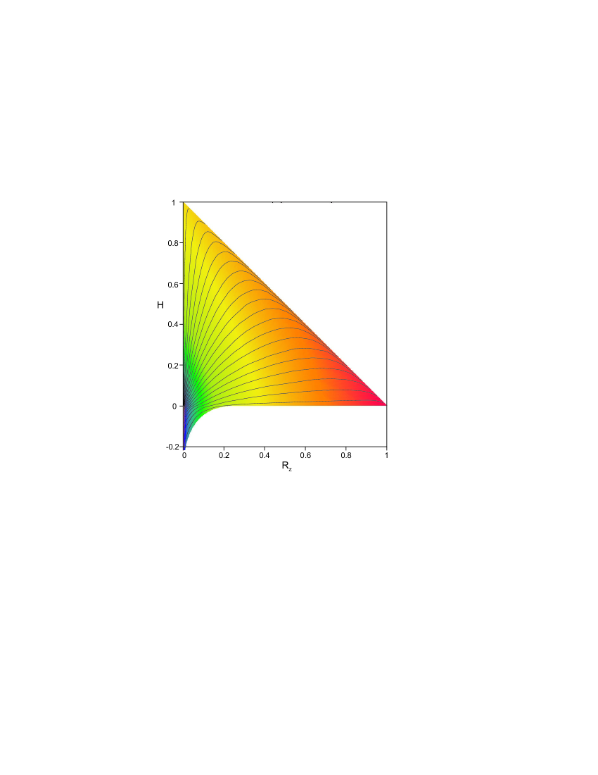
We set up an initially uniform (isotropic) distribution ($f=\mathrm{const}$) in the $\mathcal{H}-\mathcal{R}_{z}$ plane outside the capture boundary, defined by equating $\mathcal{R}_{\mathrm{lc}}$ and ${\mathcal{R}}_{\mathrm{min}}$ found from equation(12c) ($\mathcal{R}_{2}$ for saucers and $\mathcal{R}_{3}$ for tubes); a series of isolines of constant ${\mathcal{R}}_{\mathrm{min}}$ is plotted in Figure 3. We studied a range of values for both $\mathcal{R}_{\mathrm{sep}}$ and $\mathcal{R}_{\mathrm{lc}}\ll\mathcal{R}_{\mathrm{sep}}$, as well as various parameters $\alpha_{\mathrm{axi}}$ in the boundary condition (62b).

The numerical solution of equation (36) was obtained on a non-uniform rectangular grid using two different sets of coordinates, defined such that the capture boundaries are parallel to the coordinate axes (see Appendix F for details); grid sizes were typically $100-300$ in each dimension and the loss region was resolved by 10-20% of the grid cells. We advanced the solutions until time $T=1/\mathcal{D}$ to achieve a steady-state profile, from which we could extract the relation between the capture rate and the average value of $f$.

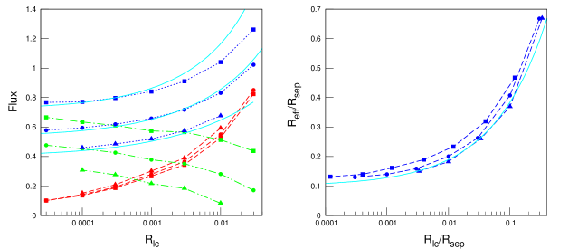
In the spherical case, the solution is controlled by two parameters (aside from $\mathcal{D}$ which scales the time): the capture boundary $\mathcal{R}_{\mathrm{lc}}$ and the boundary coefficient $\alpha$ (or $q$). As regards the steady-state profile, these two parameters are not independent, since one can always transform the problem to another (primed) one with $\alpha^{\prime}=0$ and $\mathcal{R}_{\mathrm{lc}}^{\prime}=\mathcal{R}_{0}$ (equation 47b), so the family of solution is effectively one-parametric. To compare the time-dependent solution of the axisymmetric problem to the spherical case, we introduce the concept of “equivalent spherical problem”, that is, the one-dimensional problem with the same coefficient $\alpha$ in the boundary condition as $\alpha_{\mathrm{axi}}$ in equation (62b), and with some effective capture boundary $\mathcal{R}_{\mathrm{eff}}$ chosen such that the time-dependend capture rate closely follows that of the axisymmetric problem. Our goal is then to find $\mathcal{R}_{\mathrm{eff}}$ as a function of the loss cone size $\mathcal{R}_{\mathrm{lc}}$ and degree of flattening, the latter parametrized by $\mathcal{R}_{\mathrm{sep}}$.

In the remainder of this section we present simple analytical arguments that give a qualitatively correct description of the two-dimensional numerical solution of the axisymmetric problem, and provide a fitting formula for $\mathcal{R}_{\mathrm{eff}}$.

Figure 4 shows stream lines of flux and isocontours of $f$ in a quasi-stationary 2d solution for a rather exaggerated value of $\mathcal{R}_{\mathrm{lc}}=0.003\approx 10^{-2}\mathcal{R}_{\mathrm{sep}}$. Even in this case, most of the stream lines end inside the saucer region, and that is definitely so for more realistic (smaller) values of $\mathcal{R}_{\mathrm{lc}}$. It is also clear that in the saucer region, $f$ depends mainly on $\mathcal{R}_{z}$ and is almost independent of the second coordinate, which justifies the square-root profile of $f(\mathcal{R}_{z})$ as in equation (64), but only in this region. In the tube region, for the greater part of the phase space ($\nu\equiv\mathcal{H}+\mathcal{R}_{z}\gtrsim\mathcal{R}_{\mathrm{sep}}$), the solution is close to that of the spherical problem, that is, $f(\mathcal{R})\propto\ln\mathcal{R}+\mathrm{const}$, with $\mathcal{R}\approx\nu$ experiencing only small oscillations. We can build an approximate solution by joining the two asymptotic forms at $\mathcal{R}_{\mathrm{sep}}$. A better description for the saucer region accounts for the fact that the flux in the $\mathcal{R}_{z}$ direction gradually decreases from $\mathcal{F}$ at the capture boundary to zero at $\mathcal{R}_{\mathrm{sep}}$:

$$\mathcal{F}_{\mathcal{R}_{z}}\equiv\int_{\mathcal{H}_{\mathrm{min}}}^{0}\!\!\!\!\!d\mathcal{H}\,\frac{1}{2}\langle(\Delta\mathcal{R}_{z})^{2}\rangle\mathcal{G}_{\mathrm{av}}\,\frac{\partial f}{\partial\mathcal{R}_{z}}\approx\mathcal{F}\times\left(1-\sqrt{\frac{\mathcal{R}_{z}}{\mathcal{R}_{\mathrm{sep}}}}\right).$$ (67)

$\mathcal{H}_{\mathrm{min}}(\mathcal{R}_{z})$ is the minimum value of $\mathcal{H}$, corresponding to the fixed-point saucer orbit (19b). The second, approximate equality in equation (67) is an empirical fit to the numerical 2d solution. Using the asymptotic expressions (35), it is easy to show that for $\mathcal{R}_{z}\ll\mathcal{R}_{\mathrm{sep}}$ the flux has the form (63), with the numerical coefficient $B\approx 0.4\sqrt{\mathcal{R}_{\mathrm{sep}}}$ (which is $\sim 30\%$ larger than the value used by Magorrian & Tremaine (1999)). The solution in the saucer region is obtained by solving the differential equation (67):

$$f_{\mathrm{saucer}}(\mathcal{R}_{z})=f_{\mathrm{lw}}+\frac{2\mathcal{F}}{B\,\mathcal{D}\mathcal{G}_{\mathcal{E}}}\sqrt{\mathcal{R}_{z}}\left(1-\frac{1}{2}\sqrt{\frac{\mathcal{R}_{z}}{\mathcal{R}_{\mathrm{sep}}}}\right),$$ (68)

which is a somewhat improved form of equation (64). The solution in the tube region outside $\mathcal{R}_{\mathrm{sep}}$ is approximated by

$$f_{\mathrm{tube}}(\mathcal{R})=f_{\mathrm{sep}}+\frac{\mathcal{F}}{\mathcal{D}\mathcal{G}_{\mathcal{E}}}\ln\frac{\mathcal{R}}{\mathcal{R}_{\mathrm{sep}}}\;;$$ (69)

the coefficient of the logarithmic term gives the same flux in the $\mathcal{R}$ direction as in the spherical problem, and $f_{\mathrm{sep}}\equiv f_{\mathrm{saucer}}(\mathcal{R}_{\mathrm{sep}})$. Figure 5 shows the two asymptotic expressions along with the actual numerical solution.

We compute the isotropized value $\overline{f}$ taking into account only the contribution from $f_{\mathrm{tube}}$, which introduces a fractional error of at most $\mathcal{R}_{\mathrm{sep}}$:

$$\overline{f}\approx\int_{\mathcal{R}_{\mathrm{sep}}}^{1}f_{\mathrm{tube}}(\mathcal{R})\,d\mathcal{R}\approx f_{\mathrm{sep}}+\frac{\mathcal{F}}{\mathcal{D}\mathcal{G}_{\mathcal{E}}}\left(\ln\frac{1}{\mathcal{R}_{\mathrm{sep}}}-1\right).$$ (70)

Putting all this together and expressing the relation between $\mathcal{F}$ and $\overline{\mathcal{N}}$ in terms of the coefficient $\alpha_{\mathrm{axi}}$ (62a), we obtain

$$\mathcal{F}=\frac{\mathcal{D}\,\overline{\mathcal{N}}}{\alpha_{\mathrm{axi}}+\ln(1/\mathcal{R}_{\mathrm{sep}})-1+2\sqrt{\mathcal{R}_{\mathrm{sep}}}/B}.$$ (71)

Equation (71) can be compared with equation (66) of Magorrian & Tremaine (1999): both share the property of being independent of $\mathcal{R}_{\mathrm{lc}}$, replacing it with some effective capture boundary $\mathcal{R}_{\mathrm{eff}}$ for the empty-loss-cone regime, although this effective value is different. By comparing (71) with the spherical analog (51b), we see that in our approximation, $\mathcal{R}_{\mathrm{eff}}=\mathcal{R}_{\mathrm{sep}}\exp(-1/B)\approx 0.08\mathcal{R}_{\mathrm{sep}}$. Figure 6 shows that equation (71) predicts well the flux in the numerical steady-state solutions; a better approximation to the effective capture boundary and the capture rate is

$$\mathcal{R}_{\mathrm{eff}} = \mathcal{R}_{\mathrm{sep}}\,\left(0.1+0.9\sqrt{\frac{\mathcal{R}_{\mathrm{lc}}}{\mathcal{R}_{\mathrm{sep}}}}\right),$$ (72)

$$\mathcal{F} = \frac{\mathcal{D}\,\overline{\mathcal{N}}}{\alpha_{\mathrm{axi}}+\ln(1/\mathcal{R}_{\mathrm{eff}})-1}.$$ (73)

Overall, the capture rates in the axisymmetric geometry are higher than in the spherical case with the same boundary condition $\alpha=\alpha_{\mathrm{axi}}$, but not by a large factor: in the full-loss-cone regime ($\alpha\gg 1$) they are essentially the same, while in the empty-loss-cone regime the effective boundary $\mathcal{R}_{\mathrm{eff}}$ is higher than $\mathcal{R}_{\mathrm{lc}}$, but since the flux depends on it only logarithmically, the difference is not likely to be more than a factor of a few.

Of course, more relevant is a comparison that takes into account that $\alpha$ in the spherical case may be different from $\alpha_{\mathrm{axi}}$ for the same values of $\mathcal{E}$ and $\mathcal{R}_{\mathrm{lc}}$, as noted near the end of the previous section. For the least bound stars which are in the full-loss-cone regime ($q(\mathcal{E})\gg 1$), $q_{\mathrm{axi}}\gg 1$ and $\alpha_{\mathrm{axi}}\approx\alpha\approx q$. In this case, the capture rate does not depend on the diffusion coefficient $\mathcal{D}(\mathcal{E})$ but only on the value of $\mathcal{R}_{\mathrm{lc}}$. The boundary condition (62a) states that the flux $\mathcal{F}_{\mathrm{lw}}$ is proportional to the average, isotropized value $\overline{f}\approx f_{\mathrm{lw}}$, and $\mathcal{D}$ cancels out.

In the opposite case $q(\mathcal{E})\lesssim 1$, the capture rate is limited by diffusion, and $\tilde{f}(\mathcal{R})$ is no longer close to isotropic. If $q\lesssim 1$, $\alpha_{\mathrm{axi}}$ is also $\lesssim 1$, and the denominator in the expression for the capture rate (73) tends to some constant value which depends only on $\mathcal{R}_{\mathrm{sep}}$, but not on $q$ or $\mathcal{R}_{\mathrm{lc}}$ (provided that $\mathcal{R}_{\mathrm{lc}}\ll\mathcal{R}_{\mathrm{sep}}$). It is largely irrelevant whether the boundary condition itself corresponds to the empty ($q_{\mathrm{axi}}<1$) or full-loss-wedge regime. In other words, in this diffusion-limited regime (both in spherical and axisymmetric cases) the boundary conditions (43) or (62a) determine $f_{\mathrm{lc}}$ for a given flux $\mathcal{F}_{\mathrm{lc}}$, which itself is set by the gradient of the overall steady-state profile of solution. By comparison, in the spherical case the denominator in the expression for the capture rate (51b) also depends only weakly (logarithmically) on $\mathcal{R}_{\mathrm{lc}}$ and is almost independent of $\alpha$. Therefore, the difference in capture rates between the axisymmetric and spherical problems, which results from the difference between $\ln\mathcal{R}_{\mathrm{eff}}(\mathcal{R}_{\mathrm{sep}},\mathcal{R}_{\mathrm{lc}})$ and $\ln\mathcal{R}_{\mathrm{lc}}$, is at most a factor of few in the case $q(\mathcal{E})\lesssim 1$.

6. The role of chaotic orbits

The Fokker-Planck formalism developed in the previous sections relied on the existence of three integrals of motion deep inside the SBH influence region. Apart from some special, fully integrable cases (e.g. Sridhar & Touma, 1997), most axisymmetric potentials containing central point masses are characterized by chaotic motion in the low-angular-momentum parts of phase space beyond the influence radius. Chaotic orbits still respect two integrals of the motion, $\mathcal{E}$ and $\mathcal{R}_{z}$, but in the absence of a third integral, they can in principle fill the accessible region in the meridional plane, allowing them to be captured as long as $\mathcal{R}_{z}<\mathcal{R}_{\mathrm{lc}}$. We estimate the capture rate from these orbits by the following argument, similar to an argument of Magorrian & Tremaine (1999). First we introduce the concept of draining of the loss region, arising from non-conservaton of angular momentum without any relaxation effects, then estimate the role of relaxation, and finally discuss the combined effects of draining and relaxation.

Assume that the chaotic orbits occupy a region in the $\mathcal{R}-\mathcal{R}_{z}$ plane with $\mathcal{R}<\mathcal{R}_{\mathrm{ch}}$. The value of $\mathcal{R}_{\mathrm{ch}}$ plays the same role as $\mathcal{R}_{\mathrm{sep}}$ inside the radius of influence, and is comparable to it for the same degree of flattening. Furthermore, we assume that every chaotic orbit with a given $\mathcal{R}_{z}$ can attain values of $\mathcal{R}\in[\mathcal{R}_{z}\ldots\mathcal{R}_{\mathrm{sep}}]$ with equal probability (numerical tests verify that this is a reasonable assumption). Recall that the number of stars with given $\{\mathcal{R},\mathcal{R}_{z}\}$, which may be identified with the probability of finding a star in a given interval of $d\mathcal{R}d\mathcal{R}_{z}$, is $d\mathcal{N}=\mathcal{G}_{\mathrm{sph}}\,f(\mathcal{R},\mathcal{R}_{z})\,d\mathcal{R}\,d\mathcal{R}_{z}$, with $\mathcal{G}_{\mathrm{sph}}$ given by equation (31). Then the fraction of time such an orbit spends below the capture boundary is $(\sqrt{\mathcal{R}_{\mathrm{lc}}}-\sqrt{\mathcal{R}_{z}})/\sqrt{\mathcal{R}_{\mathrm{ch}}}$, and this is essentially the probability of being captured during one radial period (assuming the full-loss-cone boundary condition, i.e. that the change in angular momentum during one period is much larger than the capture boundary, which is reasonable for chaotic orbits).

Next we evaluate the time-dependent rate of capture of stars from chaotic orbits. From the above argument it follows that we need to consider $f(\mathcal{R}_{z})$ decaying exponentially at every value of $\mathcal{R}_{z}$ from its initial value $f_{\mathrm{init}}$, but with a different rate:

$$f(\mathcal{R}_{z},t)=f_{\mathrm{init}}\,\exp\left[-\frac{t}{T_{\mathrm{rad}}}\frac{\sqrt{\mathcal{R}_{\mathrm{lc}}}-\sqrt{\mathcal{R}_{z}}}{\sqrt{\mathcal{R}_{\mathrm{ch}}}}\right].$$

The total number of chaotic orbits with $\mathcal{R}_{z}<\mathcal{R}_{\mathrm{lc}}$ and their capture rate is then given by

$$N_{\mathrm{ch}}(\mathcal{E},t)\,d\mathcal{E} = \int_{0}^{\mathcal{R}_{\mathrm{lc}}}\mathcal{G}_{\mathcal{E}}f(\mathcal{R}_{z},t)\left(\sqrt{\mathcal{R}_{\mathrm{ch}}/\mathcal{R}_{z}}-1\right)d\mathcal{R}_{z}\,d\mathcal{E}$$ (74a)

$$\approx \mathcal{G}_{\mathcal{E}}f_{\mathrm{init}}\,2\sqrt{\mathcal{R}_{\mathrm{ch}}\mathcal{R}_{\mathrm{lc}}}\,\frac{1-\exp(-2\tau)}{2\tau}\,d\mathcal{E},$$

$$\mathcal{F}_{\mathrm{ch}}(\mathcal{E},t)\,d\mathcal{E} = \frac{\mathcal{G}_{\mathcal{E}}f_{\mathrm{init}}\mathcal{R}_{\mathrm{lc}}}{T_{\mathrm{rad}}}\,\frac{1-(2\tau+1)\exp(-2\tau)}{2\tau^{2}}\,d\mathcal{E},$$

where

$$\tau\equiv t/T_{\mathrm{drain}}\;,\quad T_{\mathrm{drain}}\equiv 2T_{\mathrm{rad}}\sqrt{\mathcal{R}_{\mathrm{ch}}/\mathcal{R}_{\mathrm{lc}}}.$$ (75)

From here it is clear that if we identify $f_{\mathrm{init}}$ with the initial value of the distribution function in the loss cone $f_{\mathrm{lc}}$, then the capture rate is initially equal to the draining rate of a uniformly populated loss cone (48). In particular, when $f_{\mathrm{init}}=\overline{f}$, we recover the standard, full-loss-cone draining rate, regardless of the value of $\mathcal{R}_{\mathrm{ch}}$. On the other hand, the draining time does depend on $\mathcal{R}_{\mathrm{ch}}$, since the number of stars in the chaotic region to be drained is $2\sqrt{\mathcal{R}_{\mathrm{ch}}/\mathcal{R}_{\mathrm{lc}}}$ times larger than the number of stars in the loss cone, therefore the draining time is longer than the radial period by the same factor. At times much longer than the draining time, the capture rate declines as $t^{-2}$, not exponentially, since it is dominated by the draining of chaotic orbits with $\mathcal{R}_{\mathrm{lc}}-\mathcal{R}_{z}\ll\mathcal{R}_{\mathrm{lc}}$.

There is a great deal of similarity between the capture rates from the loss wedge of the saucer region of phase space for regular orbits within the radius of influence, and the chaotic region outside it. The details of draining are somewhat different (in particular, for the regular orbits the draining rate declines as $t^{-3}$, as noted by Magorrian & Tremaine (1999)), but since the draining time for saucer orbits is usually much shorter than a Hubble time, we ignore that distinction and adopt the same expressions for them as for chaotic orbits. In both cases, the local boundary condition for the loss region corresponds to the full loss cone (62a), at least for the case $q_{\mathrm{axi}}>1$ relevant for all but the most tightly bound orbits. However, the global shape of the steady-state solution depends on whether the overall flux into the low angular momentum region is limited by diffusion ($q(\mathcal{E})\lesssim 1$) or not. In the first case, the steady-state solution will still have a logarithmic form for $\mathcal{R}\gtrsim\mathcal{R}_{\mathrm{ch}}$ or $\mathcal{R}_{\mathrm{sep}}$, corresponding to some effective capture boundary $\mathcal{R}_{\mathrm{eff}}$, and the capture rate depends on this effective boundary only logarithmically. In the latter case, the capture rate is essentially the full loss cone rate for an isotropic distribution function. The latter case, however, is rarely attained because $q(\mathcal{E})$ rapidly drops with decreasing binding energy. On the other hand, if the draining time for chaotic orbits is comparable to the Hubble time, then their capture rate may still be quite high even in the absence of relaxation, provided that the initial value $f_{\mathrm{init}}$ of the distribution function inside the chaotic region was not much different from the isotropic value $\overline{f}$.

The combined effect of draining and relaxation may be approximately accounted for by the following recipe. Let $\mathcal{F}_{\mathrm{rel}}(\mathcal{E},t)\,d\mathcal{E}$ be the capture rate per unit energy from the Fokker-Planck equation with initial conditions corresponding to the loss region being initially empty (i.e. the solution considered in § 5). Since the loss region initially may have some nonzero value of $f$, $0\leq f_{\mathrm{init}}\leq\overline{f}$, the phase-space gradient of $f$ near the loss region boundary will be less than arising in the Fokker-Planck solution, and the capture rate from relaxation alone may also be lower. We approximate the total capture rate by the sum of the draining rate $\mathcal{F}_{\mathrm{drain}}$ and the collisional flux $\mathcal{F}_{\mathrm{rel}}$ multiplied by $1-N_{\mathrm{ch}}(t)/N_{\mathrm{ch,0}}$, where $N_{\mathrm{ch,0}}$ is the number of chaotic orbits at $t=0$ with $f_{\mathrm{init}}=\overline{f}$. This expression is used to compare Fokker-Planck models against $N$-body simulations in §8 and to compute the capture rates for real galaxies in §9. It is important to note that the effective capture boundary $\mathcal{R}_{\mathrm{eff}}$ defined in (72), as the parameter controlling the overall shape of the steady-state solution and the gradient of the distribution function (and hence the capture rate due to diffusion), is not the same as the size of the loss region ($\sqrt{\mathcal{R}_{\mathrm{sep}}\mathcal{R}_{\mathrm{lc}}}$ for saucer orbits, $2\sqrt{\mathcal{R}_{\mathrm{ch}}\mathcal{R}_{\mathrm{lc}}}$ for chaotic orbits) which determines the draining time. The former, being a fixed fraction of $\mathcal{R}_{\mathrm{sep}}$ ($\mathcal{R}_{\mathrm{ch}}$), is usually much larger than the latter.

These results will be used in §8 when we compare the model predictions with the results of $N$-body simulations.

7. Triaxiality

For completeness, and to put our results in a broader context, we briefly discuss the case when the stellar cusp around the SBH is triaxial. Triaxial potentials support two distinct familes of tube orbits, circulating about the long and short axes of the triaxial figure (Merritt & Vasiliev, 2011). In addition, there is a new class of centrophilic regular orbits, the pyramids (Merritt & Valluri, 1999, Figure 11). The defining feature of pyramids is that ${\mathcal{R}}_{\mathrm{min}}=0$ for all of them, and a star on such an orbit will eventually find its way into the SBH even without the assistance of collisional relaxation. The fraction of phase space occupied by pyramids is comparable to that of saucer orbits, i.e. $\sim\mathcal{R}_{\mathrm{sep}}$. Outside the radius of influence, the regular pyramid orbits are mostly replaced by chaotic orbits, which are however still centrophilic (Poon & Merritt, 2001).

Table 1Comparison of three geometries

	Spherical	Axisymmetric	Triaxial
Fraction of stars
with ${\mathcal{R}}_{\mathrm{min}}<\mathcal{R}_{\mathrm{lc}}$	$\mathcal{R}_{\mathrm{lc}}$	$\sqrt{\mathcal{R}_{\mathrm{lc}}\mathcal{R}_{\mathrm{sep}}}$	$\mathcal{R}_{\mathrm{sep}}$
Draining time $T_{\mathrm{drain}}$	$T_{\mathrm{rad}}$	$\gtrsim T_{\mathrm{prec}}$	$\gg T_{\mathrm{prec}}$

Table 1 summarizes the three cases. The number of stars that potentially can be captured (loss region, stars with ${\mathcal{R}}_{\mathrm{min}}<\mathcal{R}_{\mathrm{lc}}$) increases with decreasing symmetry, however the instantaneous number of stars in the loss cone is the same (the fraction of time a star on a loss region orbit actually has instantaneous $\mathcal{R}<\mathcal{R}_{\mathrm{lc}}$ exactly balances that). Consequently, the survival time of these stars also increases with decreasing symmetry: $T_{\mathrm{drain}}$ is larger than $T_{\mathrm{rad}}$ by the same factor as the number of stars in the loss region versus the loss cone, assuming a full-loss-cone draining rate.

In the absence of relaxation, the loss region is rapidly depleted in both spherical and axisymmetric cases (the latter – except for the most massive SBHs), but in the triaxial case the draining time of the loss region may be comparable to or even exceed galaxy lifetimes (Merritt & Vasiliev (2011); in that paper a rather small departure from spherical symmetry was considered; for $\mathcal{R}_{\mathrm{sep}}\sim 0.1$ or for more massive SBHs the time will be longer.) If, as suggested by Merritt & Poon (2004) and Holley-Bockelmann & Sigurdsson (2006), the capture of stars from centrophilic orbits (both regular pyramids inside the radius of influence, and chaotic orbits outside it) can sustain a full-loss-cone feeding rate for an initially isotropic distribution of stars, then it will remain near this level for a time $\sim T_{\mathrm{drain}}$. For stellar systems older than that, it is necessary to take 2-body relaxation into account, and the outcome will probably be similar to what happens in the $q_{\mathrm{axi}}>1,q<1$ regime of the axisymmetric problem: reshuffling of stars in angular momentum near the loss cone boundary due to nonspherical torques is efficient enough to keep the loss cone full, but the value of $f_{\mathrm{lc}}$ near loss cone is much smaller than the average (isotropized) value $\overline{f}$, because the supply of stars into the low-$\mathcal{R}$ region is limited by the diffusion from higher $\mathcal{R}$. Extrapolating the estimates of draining times for axisymmetric galactic models from §9 to the triaxial case, one may conclude that for most massive galaxies the lifetime of centrophilic orbits may indeed be longer than Hubble time, provided that the triaxiality is not destroyed by the effects of chaos (Merritt & Quinlan, 1998).

We stress that genuinely centrophilic orbits exist only in the triaxial case, since in the axisymmetric geometry the conservation of $L_{z}$ precludes orbits from reaching arbitrarily small radii. However, some degree of non-axisymmetry is to be expected in every real galaxy.

8. Comparison with $N$-body simulations

To test the predictions of the Fokker-Planck models, we carried out a series of $N$-body integrations of both spherical and flattened models of galaxies containing central point masses. The model mass distribution was a flattened modification of the spherical Dehnen (1993) profile:

$$\rho(\boldsymbol{x})=\frac{4\pi}{(3-\gamma)}\frac{1}{r^{\gamma}(1+r)^{4-\gamma}}\left(1+\epsilon_{d}\left[\frac{z^{2}}{r^{2}}-\frac{1}{3}\right]\right),$$

with $\gamma=3/2$. This model deviates from the scale-free profile of equation (1a) at large radii but is close to it inside $r_{\mathrm{infl}}$.

Our Fokker-Planck models are valid only for scale-free density profiles and at radii inside the SBH sphere of influence. Similar $N$-body studies (Brockamp et al., 2011; Fiestas et al., 2012) typically assign a mass to the SBH particle of $\sim 10^{-3}-10^{-2}$ times the mass in stars, similar to the observed ratio. Here (as in Komossa & Merritt, 2008) we adopt larger values for this ratio in order to study in detail the region inside the influence sphere. We used two values for $M_{\bullet}$: $0.1$ and $0.02$ times the mass in stars (the latter set to unity). In order to simulate various evolutionary regimes (e.g. empty/full loss cone) we varied the radius $r_{\mathrm{lc}}$ at which stars are captured between $10^{-5}$ and $2\times 10^{-4}$ (in units of the Dehnen-model scale length), and we also varied the number of particles in the system: $N=2.5\times 10^{4},10^{5}$ and $2.5\times 10^{5}$. We stress that in no case would our models correspond to real galaxies (the capture radius is too large and the number of stars too small), but once we understand the dependence of the evolution on these parameters, we can scale the results to real galaxies. We summarize the parameters of our models in Table 2.

Table 2Parameters of the $N$-body and Fokker-Planck models

$N$ is the number of particles, $r_{\mathrm{lc}}$ is the loss cone radius (distance to SBH at which stars are captured), $T_{\mathrm{rel}}$ is the central relaxation time defined in equation (55), $T_{\mathrm{sim}}$ is the duration of the simulation, $\ln\Lambda$ is the Coulomb logarithm, $r_{\mathrm{m}}$ is the influence radius, $r_{\mathrm{local(global)}}$ are radii corresponding to energy $\mathcal{E}_{\mathrm{local(global)}}$ of transition between empty and full-loss-cone regimes for the spherical problem defined at the end of §4.1, $N_{\mathrm{capt}}$ is the total number of particles captured by the end of integration (separately for spherical and axisymmetric case with axis ratio of 0.75, and for Fokker-Planck and $N$-body models). $N_{\mathrm{capt}}$, spherical $N_{\mathrm{capt}}$, flattened Model $N$ $M_{\bullet}$ $r_{\mathrm{lc}}$ $T_{\mathrm{rel}}$ $T_{\mathrm{sim}}$ $\ln\Lambda$ $r_{\mathrm{m}}$ $r_{\mathrm{local(global)}}$ F-P $N$-body F-P $N$-body M1 $10^{5}$ 0.1 $10^{-4}$ 250 100 8 0.5 0.09 (0.45) 560 620 990 930 M2 $10^{5}$ 0.1 $10^{-5}$ 250 100 8 0.5 0.03 (0.09) 190 240 300 280 M3 $2.5\times 10^{4}$ 0.1 $10^{-5}$ 75 50 6.6 0.5 0.017 (0.045) 45 45 55 60 M4 $2.5\times 10^{5}$ 0.1 $2\times 10^{-4}$ 550 100 8.9 0.5 0.25 (4.5) 1160 1260 2550 2540 M5 $2.5\times 10^{5}$ 0.02 $10^{-5}$ 60 50 7.3 0.14 0.013 (0.037) 270 320 380 370

For the flattened models we adopted a density axis ratio of $p=0.75$, which corresponds to $\mathcal{R}_{\mathrm{sep}}\approx 0.29$ via equations (1e), (11b). We did not vary this parameter since the foregoing analysis indicated a rather weak dependence of the flux on $\mathcal{R}_{\mathrm{sep}}$ (e.g. equation 73).

The flattened models were constructed with the Schwarzschild (1979) orbit superposition method, in the implementation described in Vasiliev (2013), using $\sim 10^{5}$ orbits. While there is a unique two-integral distribution function $f(\mathcal{E},L_{z})$ that self-consistently reproduces a given $\rho(R,z)$ (Lynden-Bell, 1962; Hunter & Qian, 1993), there are infinitely many three-integral distribution functions (e.g. Dehnen & Gerhard, 1993). In order to construct models that were “most similar” to isotropic spherical models, we chose the orbital weights in such a way as to minimize a global measure of the “velocity anisotropy” $\beta\equiv 1-(\sigma_{\theta}^{2}+\sigma_{\phi}^{2})/(2\sigma_{r}^{2})$. The resultant models are characterized by a non-trivial dependence of $f$ on the third integral, since in a two-integral, $f(E,L_{z})$ model, velocities are forced to be isotropic in the meridional plane only, i.e. $\sigma_{\theta}^{2}=\sigma_{r}^{2}$, and $\beta\neq 0$ in general. Among the numerical checks that we carried out was to construct spherical models using both orbital superposition, as well as Eddington’s inversion formula; no noticeable difference was found in the $N$-body evolution.

The models were evolved using the direct-summation $N$-body code $\phi$GRAPEch (Harfst et al., 2008), which uses algorithmic regularization (Mikkola & Merritt, 2006, 2008) to increase the speed and accuracy of particle advancement near the SBH, and includes an option for capturing particles that pass within a specified distance from the SBH; the mass of captured stars is added to $M_{\bullet}$. Integrations were carried out both on GRAPE workstations and with the GPU-accelerated SAPPORO library (Gaburov et al., 2009). The accuracy parameter of the Hermite integrator was set to $\eta=0.01$ and the gravitational softening length $\epsilon$ was set to zero. We used purely Newtonian gravity, as the influence of relativistic effects on the total capture rate (due mainly to stars with $a\sim r_{\mathrm{m}}$) is likely to be negligible (Appendix A). The integration time $T_{\mathrm{sim}}$ in $N$-body units was chosen to be a substantial fraction of the central relaxation time $T_{\mathrm{rel}}$ (55), but not longer, in order to avoid significant changes in the density profile. In all integrations, the mass of captured stars was a small fraction of $M_{\bullet}$, therefore we did not change $r_{\mathrm{lc}}$ as a function of time. A star was considered to be captured if its angular momentum near periapsis passage was less than $L_{\mathrm{lc}}=r_{\mathrm{lc}}\sqrt{2(GM_{\bullet}/r_{\mathrm{lc}}-\mathcal{E})}\approx\sqrt{2GM_{\bullet}r_{\mathrm{lc}}}$; we used the latter approximation which is valid for highly eccentric orbits. Angular momentum is preferable to periapsis radius as a condition for capture since $L$ can be computed far from the SBH particle where ambiguities due to GR are negligible.

Corresponding Fokker-Planck models were constructed in the following way. We used Eddington’s formula to obtain the isotropized distribution function $f(\mathcal{E})$ for the given density profile. For each value of energy the diffusion in angular momentum (for the spherical case) or in the $\mathcal{H}-\mathcal{R}_{z}$ space (in the flattened case) was considered using the analytical expressions for the time-dependent one-dimensional solution in terms of Bessel functions (Milosavljević & Merritt, 2003), or the steady-state expressions (51a-b). For the flattened system we used the equivalent 1d prescription from § 5, with $\alpha_{\mathrm{axi}}$ and $\mathcal{R}_{\mathrm{eff}}$ given by equations (62b), (72). We also accounted for the draining of chaotic orbits and the loss wedge using the expressions (LABEL:eq_Fchaotic), (75) for the draining rate of an initially full loss region (i.e. isotropic distribution) and the approximate combination of draining and relaxation capture rates described at the end of § 6; the fraction of chaotic orbits $\mathcal{R}_{\mathrm{ch}}$ was set equal to $\mathcal{R}_{\mathrm{sep}}$. Thus our Fokker-Planck models represent the same starting conditions as the $N$-body integrations.

We used a number of criteria for comparing the results from the Fokker-Planck and $N$-body models. Below we present comparison for some of these criteria evaluated for model M1 (spherical and axisymmetric cases), although the results were similar for other models.

Figure 7.— Comparison of theoretical diffusion coefficients with results from the $N$-body simulations (spherical Dehnen model with $M_{\bullet}=0.1$, $N=10^{5}$). Theoretical coefficients are shown by the solid ($\mathcal{R}$) and dashed ($\mathcal{E}$) curves. The diffusion coefficient in energy has been shifted downward by two decades to avoid overlap.

Figure 8.— Change in squared angular momentum during the final orbit before capture, for spherical (left) and axisymmetric (right) models with $M_{\bullet}=0.1$, $N=10^{5}$, $r_{\mathrm{lc}}=10^{-4}$. Solid lines are predictions from loss cone theory: equation (76) for the spherical case, equation (78) for the axisymmetric case; the latter should be regarded as an upper limit for the reasons discussed in the text. Horizontal dashed line is the loss cone boundary, $L^{2}=2GM_{\bullet}r_{\mathrm{lc}}$

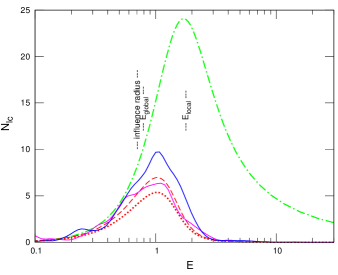
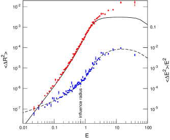
The first indicator is the rate of relaxation in energy and angular momentum. In the simulations, we sorted all particles in initial $\mathcal{E}$ and $\mathcal{R}$ and divided them into 100 bins, then computed $(\Delta\mathcal{R})^{2}$ and $(\Delta\mathcal{E})^{2}/\mathcal{E}^{2}$ for each particle and averaged these values within each bin. For a diffusive process, these quantities should grow linearly with time and so we fitted the time dependence with a straight line and took the slope of this fit as the measured value of $\langle(\Delta\mathcal{E})^{2}\rangle,\langle(\Delta\mathcal{R})^{2}\rangle$. Theoretical diffusion coefficients were computed by averaging the local coefficients over the volume of phase space accessible at a given energy (equation E4). The comparison between these theoretical coefficients and the values measured from the simulations is shown in Figure 7 for the (spherical) model M1. The Coulomb logarithm is the only adjustable parameter in this comparison, and the best agreement was obtained setting it roughly equal to the logarithm of the number of particles inside the influence radius, $\ln\Lambda\approx\ln(0.3M_{\bullet}/m_{\star})$ (e.g. Merritt, 2013, equation 5.35). Agreement was found to be good beyond and just inside the SBH sphere of influence, $\mathcal{E}\approx 1$, while at smaller radii (larger binding energies) relaxation in angular momentum was found to be faster than predicted, which may be an indication of resonant relaxation (Rauch & Tremaine, 1996), although the diffusion rate was not as high as measured by Eilon, Kupi & Alexander (2009). For a power-law cusp with $\gamma=3/2$, both $\langle(\Delta\mathcal{R})^{2}\rangle$ and $\langle(\Delta\mathcal{E})^{2}\rangle/\mathcal{E}^{2}$ should tend to constant limits for $\mathcal{E}\to\infty$. Since the number of stars in the simulations is finite and there is a maximum value of the binding energy, $\mathcal{E}\approx 100$, for an $N=10^{5}$ particle system, we introduced an upper energy cutoff in the distribution function in computing the theoretical coefficients (cf. Bar-Or et al., 2013, Appendix D), which results in the decline of the coefficients at large $\mathcal{E}$. We did not attempt to study resonant relaxation in more detail since it is not well described by our Fokker-Planck formalism and more sophisticated statistical models may be needed. In any case, the enhancement in the capture rate due to resonant relaxation is expected to be small due to the small number of particles at high binding energies (Hopman & Alexander, 2006).

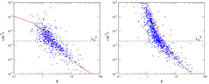
Next we compare the properties of captured particles and the population of the loss cone with the predictions of the Fokker-Planck models, in both spherical and axisymmetric models. For every captured star, we recorded the energy and angular momentum at the moment of capture, then looked back to find their changes since the previous periapsis passage. Figure 8 plots changes in squared angular momentum during the final orbit versus particle energy and compares it with the expected (average) change due to diffusion. In the case of spherical models (Figure 8a), those changes were predicted in terms of $q(\mathcal{E})$ (42) as follows:

$$\Delta\mathcal{R} = \sqrt{\mathcal{D}_{RR}\,T_{\mathrm{rad}}}=\sqrt{\left(\frac{\mathcal{D}_{RR}}{\mathcal{R}}\right)(\mathcal{R}_{\mathrm{lc}}+\Delta\mathcal{R})\,T_{\mathrm{rad}}}=$$

$$= \sqrt{q\mathcal{R}_{\mathrm{lc}}(\mathcal{R}_{\mathrm{lc}}+\Delta\mathcal{R})}=q\mathcal{R}_{\mathrm{lc}}\frac{1+\sqrt{1+4q^{-1}}}{2},$$

$$(\Delta L)^{2} = L_{\mathrm{circ}}^{2}\Delta\mathcal{R}=2GM_{\bullet}r_{\mathrm{lc}}\,q\frac{1+\sqrt{1+4q^{-1}}}{2}.$$ (76b)

In spite of the substantial scatter, the measured angular momentum changes are well described by this approximation.

For the axisymmetric case (Figure 8b) the angular momentum changes during the final orbit are higher due to torques from the flattened potential. We can estimate $\langle\Delta\mathcal{R}\rangle$ by approximating the time evolution of $\mathcal{R}$ (2) near the minimum as a parabola, taking ${\mathcal{R}}_{\mathrm{max}}=\mathcal{R}_{\mathrm{sep}},{\mathcal{R}}_{\mathrm{min}}=0$ and evaluating the difference

$$\Delta\mathcal{R}=({\mathcal{R}}_{\mathrm{max}}-{\mathcal{R}}_{\mathrm{min}})\frac{\pi^{2}}{T_{\mathrm{prec}}^{2}}\left[(T_{\mathrm{lc}}+T_{\mathrm{rad}})^{2}-T_{\mathrm{lc}}^{2}\right]\;,$$ (77)

where $T_{\mathrm{lc}}\equiv(T_{\mathrm{prec}}/\pi)\sqrt{\mathcal{R}_{\mathrm{lc}}/{\mathcal{R}}_{\mathrm{max}}}$ denotes the elapsed time after entering the loss cone until reaching the minimum $\mathcal{R}$. This estimate gives an upper limit to $\Delta\mathcal{R}$, expressed in terms of coefficient $q_{\mathrm{axi}}$ (59):

$$\Delta\mathcal{R}=\mathcal{R}_{\mathrm{lc}}\times\pi q_{\mathrm{axi}}(2q_{\mathrm{axi}}+\pi),$$ (78)

which is plotted as a solid line in Figure 8b; the measured values of $\Delta\mathcal{R}$ indeed lie below this upper limit but are higher than in the spherical case.

Figure 9.— Instantaneous number of stars in the loss cone as a function of energy. Solid curves are derived from the $N$-body simulations: top (blue) – axisymmetric; bottom (magenta) – spherical (same model as in the previous figure). Green dot-dashed curve is for a full loss cone (equation 80a with $\overline{\mathcal{N}}(\mathcal{E})$ equal to its initial value). Dotted red curve is the “real”, stationary loss cone population (equation  80b) and the dashed red curve is the time-dependent population, both for the spherical problem.

The population of the loss cone in the $N$-body simulations was computed as the instantaneous number of stars having angular momenta less than $L_{\mathrm{lc}}$. The corresponding quantity in the Fokker-Planck models is

$$N_{\mathrm{<lc}}(\mathcal{E})\,d\mathcal{E}=\int_{0}^{\mathcal{R}_{\mathrm{lc}}(\mathcal{E})}\mathcal{N}(\mathcal{E},\mathcal{R})\,d\mathcal{R}\,d\mathcal{E}.$$ (79)

We distinguish between $N_{\mathrm{full\ lc}}$ – the number of stars if their distribution in squared angular momentum is uniform (i.e. if the loss cone is full and the value of distribution function $\mathcal{N}_{\mathrm{lc}}$ for $\mathcal{R}<\mathcal{R}_{\mathrm{lc}}$ is the same as the isotropic value $\overline{\mathcal{N}}$), and $N_{\mathrm{real\ lc}}$ – the number of stars if $\mathcal{N}(\mathcal{E},\mathcal{R})$ is taken from the true solution or its quasi-steady-state approximation (equation 51a). Neglecting the variation of orbital period with $\mathcal{R}$ at given $\mathcal{E}$, the former quantity becomes

$$N_{\mathrm{full\ lc}}(\mathcal{E})\approx\mathcal{R}_{\mathrm{lc}}\overline{\mathcal{N}}(\mathcal{E}),$$ (80a)

and the latter (steady-state) is

$$N_{\mathrm{real\ lc}}=N_{\mathrm{full\ lc}}\,\frac{\exp(-\alpha)-1+\alpha}{\alpha-\ln\mathcal{R}_{\mathrm{lc}}-1},$$ (80b)

where $\alpha(q(\mathcal{E}))$ is given by (45). Figure 9 shows the distribution of loss cone stars in energy in the simulations; overplotted are curves corresponding to full and real loss cone in time-dependent and steady-state spherical Fokker-Planck solutions. We did not derive analogous expressions for the axisymmetric case, but the results from the simulations indicate that in the latter case the number of stars in the loss cone is somewhat higher than in the spherical system for energies $\mathcal{E}\geq\mathcal{E}_{\mathrm{global}}$, i.e. above the transition from full to empty-loss-cone regimes in the spherical system.

Figure 10.— Cumulative number of captured stars in the simulations (run M1) as a function of time (points), compared with predictions from the time-dependent Fokker-Planck models (dashed lines). Top (blue) curves: axisymmetric model; bottom (red/magenta) curves: spherical model.

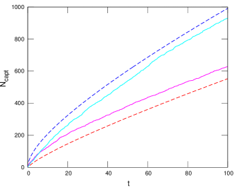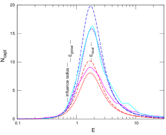
Finally, we consider the capture rate, or, rather, the cumulative number of stars captured since the beginning of the simulation as a function of time. The stationary solution of the 1d Fokker-Planck equation underestimates the capture rate at early times when the phase space density near the loss cone has not yet reached its steady-state value, so we adopted the time-dependent solution as a basis for comparison. Figure 10 shows that the capture rate decreases with time, i.e. the cumulative number of captured stars grows more slowly than linearly, as expected. Figure 11 shows the distribution of captured particles in energy, which matches the Fokker-Planck solution very well, apart from an excess of captured particles at high binding energies in the simulations, which is a consequence of the higher rate of diffusion in angular momentum discussed above (Figure 7). Overall, the capture rate for model M1 in the axisymmetric case is $\sim 50\%$ higher than for the spherical model with the same density profile, confirming the predictions of the Fokker-Planck study. The same was found to be true in the other models of Table 2: flattening was never found to make more than a factor of two difference. Moreover, models for which the transition to the full-loss-cone regime in the spherical problem occurs well within the radius of influence (M2, M3, M5) showed less difference than the model M4 which is mainly in the empty-loss-cone regime; these results are in line with theoretical predictions presented at the end of § 5.

Figure 11.— Distribution of captured stars in energy (plotted is the number of stars captured per unit time). Solid curves are from the $N$-body integrations: top (blue): axisymmetric; bottom (magenta): spherical models, in both cases with $M_{\bullet}=0.1$, $N=10^{5}$, $r_{\mathrm{lc}}=10^{-4}$ (model M1). Overplotted are predictions from the Fokker-Planck models: dotted: stationary flux (equation (51b) for the spherical case (red), equation (73) for the axisymmetric case (blue) with the effective capture boundary $\mathcal{R}_{\mathrm{eff}}$ given by equation (72)); dashed: time-dependent solution of the 1d spherical problem for the same two cases.

Figure 12.— Top panel: Distribution of captured stars (per unit of time) by orbital type for axisymmetric model M1. Dotted red: saucers; dashed green: tubes; dot-dashed blue: chaotic; solid line: total. Bottom panel: Fraction of different types of orbits in the axisymmetric Schwarzschild model M1, as a function of energy. Dotted red: saucers; dot-dashed blue: chaotic (numbers are on the right-hand ordinate); solid green: sum of these two; dashed black: cumulative mass (fraction of stars with energy $>\mathcal{E}$, numbers on the left ordinate).

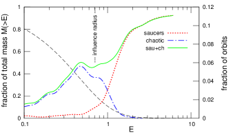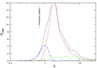
We also recorded the orbital parameters of captured stars at their final apoapsis passage and followed the orbits in the smooth potential used to construct the flattened models. Figure 12, top panel, shows that most of these stars found their way into the SBH while being on saucer orbits, a result also predicted by the axisymmetric Fokker-Planck models. The bottom panel of this figure shows that around and beyond the radius of influence, chaotic orbits play a similar role to saucers, however, in this particular model their contribution to the total capture rate is small.

As a final remark, we tested that the $N$-body models were in dynamical equilibrium by examining the evolution of Lagrangian radii of shells containing given fractions of the total mass (5%, 10%, etc.), and also the axis ratios of the models. In integrations with captures disabled, these did not change apart from small fluctuations. When captures were enabled, Lagrangian radii expanded slightly with respect to time (corresponding to energy input from the SBH), while the axis ratios did not change appreciably. The SBH particle did not remain precisely at the model center but rather experienced Brownian motion (Merritt, Berczik & Laun, 2007); however the amplitude was at least an order of magnitude smaller than the influence radius. Brockamp et al. (2011) found no substantial differences in capture rate between simulations with fixed and wandering SBHs.

9. Estimates for real galaxies

Figure 13.— Estimates of the capture rate $\dot{M}$ as a function of SBH mass $M_{\bullet}$ and of the parameters defining the galaxy. Left panel: Predictions from Fokker-Planck models for galaxies with inner density cusp slope $\gamma=1.5$ for $M_{\bullet}\leq 10^{8}\,M_{\odot}$ and $\gamma=1$ for $M_{\bullet}\geq 10^{8}\,M_{\odot}$ (the discontinuity corresponds to $\sim 3$ times higher rates for more concentrated galaxies). Galaxy models are scaled to match the $M_{\bullet}-\sigma$ relation (81) with $\alpha=8,\beta=4.5$. Solid red curves and dashed purple lines: stationary and time-dependent flux in the spherical case; dot-dashed and dotted blue lines: same for axisymmetric case with $\mathcal{R}_{\mathrm{sep}}=0.1$; double-dashed blue line: flux in the axisymmetric case with contribution from loss region draining. On average, stationary capture rates differ by a factor of 2-3 between spherical and axisymmetric cases; the time-dependent solution generally yields higher rates since it starts from an initial condition with strong gradients in the distribution function near the loss region, which may not be physically motivated and hence provides an upper limit to possible rates in real galaxies. Right panel: Comparison of stationary capture rates in the spherical case for different density cusp slopes; shaded regions correspond to uncertainty due to the range of parameters $\{\alpha,\beta\}$ in the $M_{\bullet}-\sigma$ relation (equation 81, Table 3). From top to bottom, $\gamma=2,1.5,1,0.5$. Points are taken from previous studies, as follows. Purple open boxes: Syer & Ulmer (1999); blue upward and downward triangles: Magorrian & Tremaine (1999) for the spherical and axisymmetric cases; black open and filled circles: Wang & Merritt (2004) for cored and cuspy galaxies; black double-dashed line: the analytic estimate from Wang & Merritt (2004) for a singular isothermal sphere ($\gamma=2$); red dot-dashed line: Brockamp et al. (2011) using their extrapolation from $N$-body simulations of $n=4$ Sérsic galaxy models; green crosses: Fiestas et al. (2012) for $N$-body evolution of King models scaled to Milky Way nuclear star cluster with a $\gamma=1.75$ cusp (spherical and flattened case).

Having verified that the Fokker-Planck models agree well with the $N$-body simulations in the range of parameters feasible for the latter, we now extrapolate the Fokker-Planck theory to parameters characteristic of real galaxies. To that end, we consider a family of models represented by Dehnen (1993) density profiles having inner cusp slopes $0.5\leq\gamma\leq 2$, and take the SBH mass to be $10^{-3}$ of the total galaxy mass (Merritt & Ferrarese, 2001; Marconi & Hunt, 2003). The corresponding influence radii lie well inside the break radius separating the inner $\rho\sim r^{-\gamma}$ cusp from the outer $\rho\sim r^{-4}$ profile, so that only the density normalization at the radius of influence (say) matters. That density is, in principle, an independent parameter but we fix it via the requirement that the galaxy satisfy the so-called $M_{\bullet}-\sigma$ relation linking $M_{\bullet}$ to the velocity dispersion observed near the center of the galaxy. The $M_{\bullet}-\sigma$ relation is typically written in the form

$$\log M_{\bullet}=\alpha+\beta\log(\sigma/200\,\mathrm{km\ s}^{-1}),$$ (81)

with parameters $\alpha\approx 8$, $4\lesssim\beta\lesssim 5$, depending on the details of sample selection (Table 3).

Table 3Parameters of the $M_{\bullet}-\sigma$ relation

$\alpha$	$\beta$	Reference
8.49	4.00	Merritt (1999)
8.08	3.75	Gebhardt et al. (2000)
8.22	4.86	Ferrarese & Merritt (2000)
8.13	4.02	Tremaine et al. (2002)
8.12	4.24	Gültekin et al. (2009)
8.13	5.13	Graham et al. (2011)
8.29	5.12	McConnell et al. (2011)

We scale the velocity unit of the Dehnen model by identifying the line-of-sight velocity dispersion, $\sigma_{p}(R)$, at the influence radius with the quantity $\sigma$ in equation (81); this is reasonable given that $\sigma_{p}$ is a weak function of projected radius $R$ for $r_{\mathrm{m}}\lesssim R\lesssim R_{e}$, with $R_{e}$ the half-light radius. (In the case $\gamma=2$ the central $\sigma_{p}$ in the model lacking a SBH was used.) Our models are thus defined by the two parameters $\{M_{\bullet},\gamma\}$. Setting $\alpha=8,\beta=4.5$, we have $r_{\mathrm{m}}=\{65,45,25,11\}\times(M_{\bullet}/10^{8}\,M_{\odot})^{0.56}$ pc for $\gamma=\{1/2,1,3/2,2\}$.

The radius $r_{\mathrm{lc}}$ that defines the loss sphere around the SBH is the larger of the radius of tidal disruption, $r_{\mathrm{tid}}$, and the (Newtonian) periapsis of an orbit that just continues inside the event horizon. For the eccentric orbits that dominate the flux into the SBH, the latter quantity is $\sim 8r_{\mathrm{g}}=8GM_{\bullet}/c^{2}$ for a Schwarzschild (nonrotating) SBH (Will, 2012); this is the radius of periapsis of a Keplerian orbit having the critical angular momentum. A star is tidally disrupted if the periapsis radius is less than

$$r_{\mathrm{tid}}\approx r_{\mathrm{g}}\times 2.2\eta^{2/3}\left(\frac{M_{\bullet}}{10^{8}\,M_{\odot}}\right)^{-2/3}\left(\frac{m_{\star}}{M_{\odot}}\right)^{-1/3}\frac{r_{\star}}{r_{\odot}}$$ (82)

(e.g. Merritt, 2013, equation 6.3). Here $\eta$ depends on the stellar equation of state and is $\sim 0.84$ for a solar-type main-sequence star. These disruption events, as opposed to direct captures, may be observed as optical and x-ray flares in otherwise quiescent galactic nuclei (Strubbe & Quataert, 2009). From the condition $r_{\mathrm{tid}}>8r_{\mathrm{g}}$ we find that solar-type stars on eccentric orbits are disrupted (not swallowed) if $M_{\bullet}\lesssim 1.2\times 10^{7}\,M_{\odot}$; disruption can occur for any $M_{\bullet}\lesssim 10^{8}M_{\odot}$ if the star is on a less eccentric orbit, or for Kerr SBHs even more massive than $10^{8}\,M_{\odot}$ (Kesden, 2012). Red giants or AGB stars can also be disrupted (or at least tidally limited) by SBHs more massive than $10^{8}\,M_{\odot}$ (Syer & Ulmer, 1999; MacLeod et al., 2012). In what follows, we compute the total number of events associated with a given $r_{\mathrm{lc}}$; the ratio of number of tidal disruption flares to the total number of capture events is well studied in the literature and we do not consider it separately here.

We used Fokker-Planck models to evaluate steady-state and time-dependent capture rates $\dot{M}$ for galaxies after $10^{10}$ years starting from an initially isotropic distribution function, in both the spherical and axisymmetric geometries (using our one-dimensional approximation of section 5), for $\mathcal{R}_{\mathrm{sep}}=0.1$. The latter value is meant to represent a “typical,” moderately-flattened system; the results do not strongly depend on $\mathcal{R}_{\mathrm{sep}}$. In the time-dependent calculations, the initial conditions consisted of the isotropic models with loss-cone orbits removed; as a result, these initial models are characterized by strong gradients of $f$ with respect to $L$ near the loss cone. Overall, the calculation of total capture rate is done in the same way as in the previous section.

The left panel of Figure 13 shows results for two series of models: models with a steep ($\gamma=1.5$) central cusp and $M_{\bullet}\leq 10^{8}\,M_{\odot}$; and models with shallow ($\gamma=1$) cores and $M_{\bullet}\geq 10^{8}\,M_{\odot}$. Over the entire range of $M_{\bullet}$, the steady-state capture rates differ by only a factor of $2-3$ between spherical and axisymmetric geometries, consistent with the discussion near the end of §5. This result holds for any galactic model and depends only weakly on $\mathcal{R}_{\mathrm{sep}}$. The time-dependent rates are generally higher than in the steady state, due to the strong gradients in the initial conditions. Especially for massive galaxies with long relaxation times, the approach to a steady state is slow and the flux at early stages is much higher than in equilibrium.

For the most massive SBHs ($M_{\bullet}\gtrsim 10^{9}\,M_{\odot}$) the draining time of the loss region becomes comparable to the Hubble time and the capture rate is dominated by draining of chaotic orbits (double-dashed line), reaching values up to $10^{-3}\,M_{\odot}$ yr^-1 at the upper end of the $M_{\bullet}$ range. However, this should be regarded as a strong upper limit since we do not know the initial state: for instance, if the SBH formed as the result of a merger of a binary SBH, it is very likely that the low angular momentum region of phase space will have been depleted in the course of the binary’s evolution, and the capture rates could initially be much lower than the steady-state values (Milosavljević & Merritt, 2003; Merritt & Wang, 2005).

The dependence of $\dot{M}$ on $M_{\bullet}$ for massive SBHs can be simply estimated as follows (e.g. Syer & Ulmer, 1999). The nuclei of massive galaxies are in the empty-loss-cone regime, so the flux per unit energy is roughly $\mathcal{F}(\mathcal{E})\,d\mathcal{E}\approx\mathcal{N}(\mathcal{E})\,d\mathcal{E}/\left[T_{\mathrm{rel}}(\mathcal{E})\,\ln\mathcal{R}_{\mathrm{lc}}^{-1}(\mathcal{E})\right]$. The capture rate peaks at $r\approx r_{\mathrm{m}}$ (Merritt, 2013, section 6.1.4.1) so the total flux is estimated as $\dot{M}\sim\mathcal{F}(\mathcal{E}_{\mathrm{infl}})\mathcal{E}_{\mathrm{infl}}\sim M_{\bullet}/(T_{\mathrm{rel}}\ln\mathcal{R}_{\mathrm{lc}}^{-1})\sim(m_{\star}/M_{\bullet})\,\sigma^{3}/G$. Assuming the $M_{\bullet}-\sigma$ relation, we obtain $\dot{N}\propto M_{\bullet}^{3/\beta-1}$, and even the normalization constant evaluates to a reasonable $\sim 10^{-5}\,M_{\odot}$ yr^-1 for $M_{\bullet}=10^{8}\,M_{\odot}$, despite the crudeness of the estimate.

The right panel of Figure 13 shows the uncertainties in the capture rate associated with the parameters $\alpha$ and $\beta$ in the $M_{\bullet}-\sigma$ relation (81) and the slope of the density cusp $\gamma$. Plotted are stationary capture rates for the spherical case; other values scale roughly in the same proportion. The capture rates evaluated for a selection of individual galaxies from several previous studies are also plotted for comparison. It is clear that the scatter in the derived values is fairly large, about two orders of magnitude, although a general trend of decreasing rate with increasing $M_{\bullet}$ is clear. Comparing the inverted triangles in Figure 13b with the double-dashed curve in Figure 13a, we see that our estimates for the capture rate due to draining of chaotic orbits are substantially higher than those of Magorrian & Tremaine (1999). As argued above, this is most likely an overestimate resulting from simplistic initial conditions. It is also due partly to our selection of a different relation between the capture rate and the isotropized distribution function; had we used their equation (66) instead of our equation (71), the steady-state flux in the axisymmetric case would be factor of a few lower, although it should not affect the draining rate of centrophilic orbits which starts to dominate the capture rate at $M_{\bullet}\gtrsim 10^{9}\,M_{\odot}$.

Overall, it is fair to say that our estimates predict capture rates in the range $10^{-5}-10^{-4}\,M_{\odot}$ yr^-1 for less massive galaxies, and a few$\times 10^{-6}-10^{-5}\,M_{\odot}$ yr^-1 for giant galaxies with SBH masses in excess of $10^{8}\,M_{\odot}$. This is roughly consistent with the observationally derived estimates of rates of tidal disruption flares (Donley et al., 2002; Gezari et al., 2008; van Velzen & Farrar, 2012). (Axisymmetric) nuclear flattening may increase these numbers by a factor of few, and triaxiality may have a more dramatic effect on the consumption rate of the most massive SBHs provided there are enough stars on centrophilic orbits.

One potentially important feature of axisymmetric (and triaxial) systems is that most stars are consumed in the full-loss-cone regime of boundary conditions (in spite of the fact that the angular momentum need not be isotropic). This means that stars approach the SBH with a wide distribution in periapsis radii, as opposed to “barely touching” the disruption sphere in the empty-loss-cone regime. As a consequence, many stars will be strongly tidally distorted before disruption, which may result in a distinct observational signature (Strubbe & Quataert, 2009), although more recent studies show that the difference may not be so pronounced (Stone et al., 2013).

10. Conclusions

We have considered collisional (gravitational-encounter-drive) relaxation processes near supermassive black holes (SBHs) in spherical and axisymmetric models of galactic nuclei. We derived a Fokker-Planck formalism and compared its predictions with direct $N$-body simulations of capture.

Inside the SBH radius of influence, the unperturbed motion of stars is regular, admitting three integrals of motion (energy, $z$-component of the angular momentum $L_{z}$, and secular Hamiltonian $\mathcal{H}$). There are two families of orbits, tubes and saucers; the latter exhibit large angular momentum variations and stars on saucer orbits approach much more closely to the SBH than would be expected based on their average angular momentum. Regularity of the motion allowed us to write down the orbit-averaged Fokker-Planck equation and to calculate the diffusion coefficients based on the standard formalism. We discussed the appropriate boundary conditions for capture by the SBH, and numerically solved the two-dimensional ($\mathcal{H}-L_{z}$) Fokker-Planck equation. We showed that its solution can be well approximated by an equivalent one-dimensional solution for diffusion in angular momentum, given appropriate boundary conditions. An important difference with the spherical case is that the boundary condition at the loss region typically corresponds to the full-loss-cone regime, in the sense that a change in angular momentum per one orbital period is larger than the size of the loss cone. Nevertheless, the global shape of the solution, and, consequently, the capture rate of stars, is determined by the diffusion coefficient (inversely proportional to the relaxation time), and depends only weakly on the effective size of the loss region. This treatment was not entirely self-consistent, as it did not account for resonant relaxation or for the breakdown of the orbit-averaged approximation near or beyond the radius of influence, but it nevertheless suggests a conclusion which turns out to be robust: compared with the spherical case having the same real (not effective) capture boundary, the flux into the loss cone is higher in the axisymmetric case, but not by a large factor, and only in the regime where the loss cone would be empty in the spherical system. In the axisymmetric case, most of the stars find their way into the SBH while on saucer orbits.

We also carried out a number of $N$-body integrations which were found to agree remarkably well with the corresponding Fokker-Planck models. The agreement was not limited to the number of captured stars; other quantities like the distribution of energy of the captured stars, the loss cone population, the diffusion coefficients, and the change in angular momentum during one radial period prior to capture were also found to be well reproduced. We note, however, that the angular momentum diffusion is larger in $N$-body models for stars with high binding energies (close to the SBH), which may be an indication of resonant relaxation not accounted for in the Fokker-Planck models; nevertheless, its influence on the capture rate is likely to be small.

We applied our Fokker-Planck formalism to realistic galaxies with SBH masses $M_{\bullet}=(10^{6}-10^{10})M_{\odot}$. We found that stationary capture rates are in the range $(10^{-4}-10^{-6})M_{\odot}$ yr^-1 in spherical galaxies and a factor $2-3$ higher in flattened systems, with an overall trend of decreasing event rate with increasing $M_{\bullet}$. Time-dependent solutions were found to give generally higher estimated capture rates; however, that result is likely to depend strongly on the assumed initial conditions (Merritt & Wang, 2005). In particular, for massive ($M_{\bullet}\gtrsim 10^{9}\,M_{\odot}$) SBHs in axisymmetric nuclei, the draining time of chaotic orbits just outside the radius of influence can be comparable to the Hubble time; if such orbits were not depleted by (for instance) the binary SBH that preceded the single SBH, capture rates might reach $10^{-3}\,M_{\odot}$yr^-1. Such high rates may be more relevant to triaxial galaxies in which the number of centrophilic orbits is likely to be large enough to maintain a full-loss-cone capture rate for a Hubble time.

The work was supported by the National Science Foundation via grant no. AST 1211602 and by the National Aeronautics and Space Administration via grant no. NNX10AF84G. EV acknowledges the hospitality of the Aspen Center for Physics. Codes for computing capture rates in the spherical and axisymmetric geometries can be downloaded at http:$//$td.lpi.ru$/$$\sim$eugvas$/$losscone$/$.

Appendix A Effect of relativity on the unperturbed modtion

We discuss briefly the character of the motion in axisymmetric nuclei when the lowest-order post-Newtonian (PN) corrections are included in the equations of motion. The 1PN accelerations imply an orbit-averaged rate of of periapsis advance

$$\left(\frac{d\omega}{dt}\right)_{\mathrm{GR}}=\frac{2\pi}{T_{\mathrm{rad}}}\frac{3GM_{\bullet}}{c^{2}a\mathcal{R}}$$ (A1)

(Merritt, 2013, equation (4.205)). The other elements of the osculating orbit exibit no secular variations at this PN order, and we ignore rotation of the SBH. Expressed in terms of the dimensionless time variable $\tau\equiv 2\pi t/T_{\mathrm{M}}$ defined in equation (9), the relativistic precession rate becomes

$$\left(\frac{d\omega}{d\tau}\right)_{\mathrm{GR}}=\frac{\kappa}{\mathcal{R}},\ \ \ \ \kappa\equiv 3(2-\gamma)\frac{r_{\mathrm{g}}}{a}\frac{M_{\bullet}}{M_{\star}(a)}=3(2-\gamma)(3-\gamma)\frac{r_{\mathrm{g}}}{a}\frac{M_{\bullet}}{4\pi a^{3}\rho_{\star}(a)}$$ (A2)

which can be added to the orbit-averaged equation of motion for $\omega$, equation (9). Setting $\gamma=1$ ($Q=3/2$) in the Hamiltonian (8), the two nontrivial equations of motion become

$$\frac{d\ell}{d\tau} = -\frac{3}{2}\epsilon_{p}(1-\ell^{2})\sin^{2}i\sin(2\omega),$$ (A3a)

$$\frac{d\omega}{d\tau} = \frac{\kappa}{\ell^{2}}-\left(1+\frac{2\epsilon_{p}}{3}\right)\ell+\epsilon_{p}\left[\frac{3}{\ell}\left(\cos^{2}i-\ell^{2}\right)\sin^{2}\omega\right].$$ (A3b)

If there is a fixed point, its angular momentum can be found by setting $\dot{\omega}=0$ when $\omega=\pi/2$, or

$$0=\left(1+\frac{5}{3}\epsilon_{p}\right)\ell^{4}-3\epsilon_{p}\ell_{z}^{2}-\kappa\ell.$$ (A4)

As $\kappa$ is increased from zero, the value of $\ell$ at the fixed point increases, reaching $\ell=1$ when

$$\kappa\equiv\kappa_{2}=1+\frac{5}{3}\epsilon_{p}-3\epsilon_{p}\ell_{z}^{2}.$$ (A5)

For $\kappa>\kappa_{2}$ all orbits are tubes. For $\kappa_{1}\leq\kappa\leq\kappa_{2}$, where

$$\kappa_{1}=1-\frac{4\epsilon_{p}}{3},$$ (A6)

there is one family of tubes, passing below the fixed point in the $(\mathcal{R},\omega)$ plane, and a family of saucer-like orbits that librate around the fixed point. For $\kappa<\kappa_{1}$, the separatrix encloses the fixed point and there are two families of tubes, at low and high angular momenta. In the latter case, the angular momentum associated with the separatrix at $\omega=0$ can be found by setting $\dot{\omega}=0$ in equation (A3b):

$$\mathcal{R}_{\mathrm{sep,GR}}\equiv\ell_{\mathrm{sep,GR}}^{2}=\left(\frac{3\kappa}{3-4\epsilon_{p}}\right)^{2/3}.$$ (A7)

Figure 14.— Solutions to the equations of motion (A3) for $\mathcal{R}_{z}=0.01$, $\kappa=0.02$ and $\epsilon_{p}=0.035$. The fixed point, equation (A4), is shown by the cross. There are two familes of tube orbits: tube orbits above the fixed point, which are present even when $\kappa=0$ (no GR); and tube orbits below the fixed point, having sufficiently small $\ell$ that relativistic precession quenches the effects of torques due to the flattened potential. Equation (A10) predicts $\mathcal{R}\approx 1.4\times 10^{-2}$ for the minimum $\mathcal{R}$ reached by saucers; the actual value is $\sim 2.4\times 10^{-2}$.

Since $\kappa_{1}\lesssim 1\lesssim\kappa_{2}$, saucer-like orbits are present only when

$$\frac{a}{r_{\mathrm{g}}}\gtrsim 3\frac{M_{\bullet}}{M_{\star}(a)}.$$ (A8)

Even when saucers are present, their angular momentum variations are limited by the relativistic term. A rough lower limit on the attainable angular momentum for saucers can be derived by equating the change in $\ell$ due to the torques over one GR precessional period to $\ell$:

$$\ell=\left|\frac{d\ell}{d\tau}\right|\times\left|\frac{1}{\pi}\frac{d\omega}{d\tau}\right|_{\mathrm{GR}}^{-1}$$ (A9)

which yields

$$\ell_{\mathrm{min}}\approx\frac{2}{3\pi}\frac{\kappa}{\epsilon_{p}}.$$ (A10)

Figure 14 shows numerical solutions of the equations of motion (A3) for $\mathcal{R}_{z}=0.01$ and $\kappa=0.02$; the nuclear flattening parameter has the same value as in Figure 2. The neglect of GR precession on the evolution of saucer orbits is justified if

$$\ell_{\mathrm{min}}\lesssim\sqrt{\mathcal{R}_{\mathrm{lc}}}\approx\sqrt{\frac{2r_{\mathrm{lc}}}{a}}\gtrsim 4\sqrt{\frac{r_{\mathrm{g}}}{a}}\;,$$ (A11)

where the latter inequality expresses the fact that $r_{\mathrm{lc}}=8r_{\mathrm{g}}$ for direct captures and larger than that for tidal disruptions. Requiring that $\ell_{\mathrm{min}}\lesssim 4\sqrt{r_{\mathrm{g}}/a}$ and using equations (3, A2, A10), we obtain

$$\frac{1}{2\pi\epsilon_{p}} \lesssim \frac{M_{\star}(a)}{M_{\bullet}}\sqrt{\frac{a}{r_{\mathrm{g}}}}=2\left(\frac{a}{r_{\mathrm{m}}}\right)^{\frac{7}{2}-\gamma}\sqrt{\frac{r_{\mathrm{m}}}{r_{\mathrm{g}}}}$$ (A12a)

$$\frac{a}{r_{\mathrm{m}}} \gtrsim \left(\frac{1}{2\pi\epsilon_{p}}\frac{\sigma}{c}\right)^{\frac{2}{7-2\gamma}},$$ (A12b)

where the second line approximates $r_{\mathrm{m}}\approx GM_{\bullet}/\sigma^{2}$. This is essentially the same condition that was obtained in Merritt & Vasiliev (2011) for capture of pyramid orbits. Since the quantity in the brackets is likely to be small (unless $\epsilon_{p}$ is tiny), and because most of the flux into the SBH comes from orbits with $a\approx r_{\mathrm{m}}$, equation (A12) suggests that relativity is not likely to be important for the total capture rate.

Appendix B Orbit-averaged Hamiltonian

Here we give the exact expression for the orbit-averaged Hamiltonian corresponding to the potential of equation (1).

It is convenient to express $r$ and $z$ in terms of eccentric anomaly $\eta$ rather than mean anomaly $w$ (e.g. Sambhus & Sridhar, 2000, eq.1):

$$r=a(1-e\cos\eta)\;,\;\;z=a\sqrt{1-\frac{\ell_{z}^{2}}{\ell^{2}}}\left[\sin\omega(\cos\eta-e)+\sqrt{1-e^{2}}\cos\omega\sin\eta\right]\;,\;\;e\equiv\sqrt{1-\ell^{2}}.$$

Then

$$\overline{\Phi}_{\star}\equiv\frac{1}{2\pi}\int_{0}^{2\pi}\Phi_{\star}(\mathbf{r})\,dw=\frac{1}{2\pi}\int_{0}^{2\pi}\Phi_{\star}(\mathbf{r})\,d\eta\,(1-e\cos\eta)=\Phi_{0}\left(\frac{a}{r_{0}}\right)^{2-\gamma}\,\tilde{H}(\ell,\ell_{z},\omega),$$

where $\tilde{H}$ is expressed in terms of Gauss’ hypergeometric function:

$$\tilde{H}=\left(1-\frac{\epsilon_{p}}{3}\right){}_{2}F_{1}\left(\frac{\gamma-2}{2},\frac{\gamma-3}{2};\,1;\,1-\ell^{2}\right)+\epsilon_{p}\left\{\frac{(4-\gamma)(5-\gamma)}{8}\;{}_{2}F_{1}\left(\frac{\gamma}{2},\frac{\gamma-1}{2};\,3;\,1-\ell^{2}\right)(1-\ell^{2})\sin^{2}\omega\right.$$

$$+\left.\left[{}_{2}F_{1}\left(\frac{\gamma}{2},\frac{\gamma-1}{2};\,3;\,1-\ell^{2}\right)+\frac{\gamma(\gamma-1)}{24}(1-\ell^{2})\;{}_{2}F_{1}\left(\frac{\gamma+2}{2},\frac{\gamma+1}{2};\,4;\,1-\ell^{2}\right)\right]\frac{\ell^{2}}{2}\right\}\left(1-\frac{\ell_{z}^{2}}{\ell^{2}}\right).$$ (B1)

Appendix C Relation to the Lidov-Kozai problem

Motion in the hierarchical three-body problem is often derived from a doubly-averaged Hamiltonian after expressing the equations of motion in Jacobi coordinates and retaining only the lowest-order (quadrupole) term in the perturbation potential. The “inner restricted problem” (Kozai, 1962; Lidov, 1962) assumes furthermore that the test mass orbits well inside the perturber mass. The averaged Hamiltonian describing the test particle, with an appropriately chosen unit of time, is

$$H_{\mathrm{K}}=-\frac{5}{6}+\frac{\mathcal{R}}{2}+\left(1-\frac{\mathcal{R}_{z}}{\mathcal{R}}\right)\left[\frac{5}{2}(1-\mathcal{R})\sin^{2}\omega+\frac{\mathcal{R}}{2}\right]$$ (C1)

(Merritt 2013, equation 4.315) which may be obtained from equation 8 by setting $Q=5/2$ and eliminating unity in the first bracket of the first term (equivalent to taking the limit $\epsilon_{p}\to\infty$, eliminating terms that do not contain $\epsilon_{p}$ and normalizing the unit of time to $\epsilon_{p}$). Equation (11b) then yields a value of $5/3$ for the parameter $\mathcal{R}_{\mathrm{sep}}$. As in the axisymmetric problem, motion in the Lidov-Kozai problem also exhibits two regimes: circulation in $\omega$ (corresponding to tube orbits) or libration about $\omega=\pi/2$ (analogous to saucers), the latter appearing for $\mathcal{R}_{z}<3/5$. The equation of motion for $\mathcal{R}$ (12a) is

$$\frac{\partial\mathcal{R}}{d\tau}=-2\sqrt{6}\,\sqrt{(\mathcal{R}_{1}-\mathcal{R})(\mathcal{R}-\mathcal{R}_{2})(\mathcal{R}_{3}-\mathcal{R})}\;,$$ (C2)

with the same relation between $\mathcal{R}_{1},\mathcal{R}_{2},\mathcal{R}_{3}$ as in equation (12c):

$$\mathcal{R}_{1,2} \equiv \mathcal{R}_{\star}\pm\sqrt{\mathcal{R}_{\star}^{2}-(5/3)\mathcal{R}_{z}}$$ (C3a)

$$\mathcal{R}_{3} \equiv H_{\mathrm{K}}+5/6+\mathcal{R}_{z}/2$$ (C3b)

$$\mathcal{R}_{\star} \equiv (5+5\mathcal{R}_{z}-2\mathcal{R}_{3})/6.$$ (C3c)

The case of circulation corresponds to $\mathcal{R}_{2}\leq\mathcal{R}\leq\mathcal{R}_{3}\leq\mathcal{R}_{1}$, and libration to $\mathcal{R}_{2}\leq\mathcal{R}\leq\mathcal{R}_{1}\leq\mathcal{R}_{3}$; in the latter case the relation between minimum and maximum values of $\mathcal{R}$ is the same as in equation (16), from which it follows that the librating regime exists for $\mathcal{R}_{z}<1/\mathcal{R}_{\mathrm{sep}}=3/5$. The separatrix between “tubes” and “saucers” is at $H_{\mathrm{K}}=1/6-\mathcal{R}_{z}/2$ and the fixed-point saucer has $H_{\mathrm{K}}=5/3+2\mathcal{R}_{z}-\sqrt{15\mathcal{R}_{z}}$. For comparison, in the oblate axisymmetric potential considered throughout this paper, the first regime (tube orbits) has $\mathcal{R}_{2}\leq\mathcal{R}_{3}\leq\mathcal{R}\leq\mathcal{R}_{1}$ and the second (saucers) has $\mathcal{R}_{3}\leq\mathcal{R}_{2}\leq\mathcal{R}\leq\mathcal{R}_{1}$.

Appendix D Saucer orbits beyond the sphere of influence

Beyond the influence sphere, orbits similar to the saucers can still exist in axisymmetric potentials (Richstone, 1982; Lees & Schwarzschild, 1992; Evans, 1994), but they are not describable in terms of osculating Keplerian elements. Typically such orbits are described as tube orbits that lie close to a resonance between the radial and vertical motions. To make the correspondence with our work more clear, we recast the fixed-point saucer orbit near a SBH in terms of the Cartesian variables ($R,z$), i.e. cylindrical coordinates in the meridional plane. Setting $\omega=\pi/2$ in equation (A1) yields for the fixed-point orbit that generates the saucers

$$\frac{R^{2}}{a^{2}}=\left(1-e^{2}\right)^{2}-\frac{2e\left(1-e^{2}\right)}{\sin i}\frac{z}{a}-\left(1-\frac{e^{2}}{\sin^{2}i}\right)\frac{z^{2}}{a^{2}}$$ (D1)

where it is understood that $e$ and $\cos i$ have their fixed-point values:

$$e^{2}=1-\sqrt{\mathcal{R}_{\mathrm{sep}}\mathcal{R}_{z}},\ \ \cos^{2}i=\sqrt{\frac{\mathcal{R}_{z}}{\mathcal{R}_{\mathrm{sep}}}}.$$

Equation (D1) is a hyperbola in the ($R,z$) plane, between the points

$$R_{\mathrm{max}} = (1+e)a\cos i,\ \ z_{\mathrm{max}}=(1+e)a\sin i,$$

$$R_{\mathrm{min}} = (1-e)a\cos i,\ \ z_{\mathrm{max}}=(1-e)a\sin i.$$

The curve crosses the equatorial plane at $R=a\sqrt{\mathcal{R}_{\mathrm{sep}}\mathcal{R}_{z}}=a(1-e^{2})$, the semi-latus rectum.

When the fixed-point saucer orbit first appears, at $\mathcal{R}_{z}=\mathcal{R}_{\mathrm{sep}}$, it lies in the equatorial plane ($\cos i=1,z_{\mathrm{max}}=0$) and has zero vertical thickness. For $\mathcal{R}_{z}$ values smaller than this maximum, the trajectory (D1) can be interpreted as a $1:1$ resonance between motions in the $R$ and $z$ directions.

Described in this way, saucer orbits near a SBH are seen to have very similar properties to orbits described by other authors in more general axisymmetric potentials. Lees & Schwarzschild (1992) studied orbits in scale-free axisymmetric models with logarithmic potentials, $\rho\sim r^{-2}$ and no central SBH. For models with density axis ratio $0.265$, they found that saucers first appear at $\mathcal{R}_{z}\approx 0.48$; for smaller $\mathcal{R}_{z}$ the fixed-point orbit (which they called a “reflected banana”) traces a path in the ($R,z$) plane similar to equation (D1). They noted that motion near the fixed-point orbit is regular, i.e. non-chaotic. Similar orbits were described by Richstone (1982) (who called them “pipe orbits”) and Evans (1994) in surveys of orbits in other scale-free families of oblate models.

Appendix E Local diffusion coefficients

Here we present the local (position-dependent) diffusion coefficients appearing in equation (3), expressed in the spherical coordinates $(r,\theta,\phi)$ and generalized velocities $(\mathcal{E}=-\Phi(r)-v^{2}/2$, $\mathcal{R}=\kappa\,L^{2}$, $\mathcal{R}_{z}=\kappa\,L_{z}^{2})$. We denote $\kappa\,\equiv L_{\mathrm{circ}}^{-2}(E)$, $\kappa\,^{\prime}=d\kappa\,/dE=-d\kappa\,/d\mathcal{E}$, $\mathcal{Q}=1+(v^{2}/2)(\kappa^{\prime}/\kappa)$.

$$\langle\Delta\mathcal{E}\rangle = -v\langle\Delta v_{\|}\rangle-\frac{1}{2}\langle\Delta v^{2}_{\|}\rangle-\frac{1}{2}\langle\Delta v^{2}_{\bot}\rangle,$$ (E1)

$$\langle\Delta\mathcal{R}\rangle = 2\mathcal{R}\mathcal{Q}\frac{\langle\Delta v_{\|}\rangle}{v}+\left(\frac{v^{4}}{2}\frac{\kappa\,^{\prime\prime}}{\kappa\,}+5\mathcal{Q}-4\right)\mathcal{R}\frac{\langle\Delta v^{2}_{\|}\rangle}{v^{2}}+\left(\mathcal{Q}-\frac{3}{2}+\frac{v^{2}}{v^{2}-v_{r}^{2}}\right)\mathcal{R}\frac{\langle\Delta v^{2}_{\bot}\rangle}{v^{2}},$$

$$\langle\Delta\mathcal{R}_{z}\rangle = 2\mathcal{R}_{z}\mathcal{Q}\frac{\langle\Delta v_{\|}\rangle}{v}+\left(\frac{v^{4}}{2}\frac{\kappa\,^{\prime\prime}}{\kappa\,}+5\mathcal{Q}-4\right)\mathcal{R}_{z}\frac{\langle\Delta v^{2}_{\|}\rangle}{v^{2}}+\left(\frac{\mathcal{R}\,\sin^{2}\theta}{2\mathcal{R}_{z}}\,\frac{v^{2}-v_{\phi}^{2}}{v^{2}-v_{r}^{2}}+\mathcal{Q}-1\right)\mathcal{R}_{z}\,\frac{\langle\Delta v^{2}_{\bot}\rangle}{v^{2}},$$

$$\langle(\Delta\mathcal{E})^{2}\rangle = v^{2}\langle\Delta v^{2}_{\|}\rangle,$$

$$\langle(\Delta\mathcal{R})^{2}\rangle = 4\mathcal{R}^{2}\mathcal{Q}^{2}\frac{\langle\Delta v^{2}_{\|}\rangle}{v^{2}}+2\mathcal{R}^{2}\frac{v_{r}^{2}}{v^{2}-v_{r}^{2}}\,\frac{\langle\Delta v^{2}_{\bot}\rangle}{v^{2}},$$

$$\langle(\Delta\mathcal{R}_{z})^{2}\rangle = 4\mathcal{R}_{z}^{2}\mathcal{Q}^{2}\frac{\langle\Delta v^{2}_{\|}\rangle}{v^{2}}+2\mathcal{R}\mathcal{R}_{z}\,\sin^{2}\theta\,\frac{v^{2}-v_{\phi}^{2}}{v^{2}-v_{r}^{2}}\,\frac{\langle\Delta v^{2}_{\bot}\rangle}{v^{2}},$$

$$\langle\Delta\mathcal{E}\Delta\mathcal{R}\rangle = -2\mathcal{R}\mathcal{Q}\langle\Delta v^{2}_{\|}\rangle,$$

$$\langle\Delta\mathcal{E}\Delta\mathcal{R}_{z}\rangle = -2\mathcal{R}_{z}\mathcal{Q}\langle\Delta v^{2}_{\|}\rangle,$$

$$\langle\Delta\mathcal{R}\Delta\mathcal{R}_{z}\rangle = 4\mathcal{R}\mathcal{R}_{z}\mathcal{Q}^{2}\frac{\langle\Delta v^{2}_{\|}\rangle}{v^{2}}+2\mathcal{R}\mathcal{R}_{z}\frac{v_{r}^{2}}{v^{2}-v_{r}^{2}}\,\frac{\langle\Delta v^{2}_{\bot}\rangle}{v^{2}}.$$

These coefficients have been expressed in terms of velocity diffusion coefficients for $\{v_{\|},v_{\bot}\}$ via integrals of the distribution function $f(\mathcal{E}_{f})$ describing the field stars (of mass $m_{\star}$) using the relative potential $\Psi\equiv-\Phi$:

$$v\langle\Delta v_{\|}\rangle = \textstyle-\left(1+\frac{m}{m_{\star}}\right)I_{1/2},$$ (E2)

$$\langle\Delta v^{2}_{\|}\rangle = \textstyle\frac{2}{3}\left(I_{0}+I_{3/2}\right),$$

$$\langle\Delta v^{2}_{\bot}\rangle = \textstyle\frac{2}{3}\left(2I_{0}+3I_{1/2}-I_{3/2}\right),$$

where

$$I_{0} \equiv 16\pi^{2}G^{2}m_{\star}^{2}\ln\Lambda\int_{0}^{\mathcal{E}}d\mathcal{E}_{f}\,f(\mathcal{E}_{f}),$$ (E3)

$$I_{n/2} \equiv 16\pi^{2}G^{2}m_{\star}^{2}\ln\Lambda\int_{\mathcal{E}}^{\Psi(r)}d\mathcal{E}_{f}\,f(\mathcal{E}_{f})\left(\frac{\Psi-\mathcal{E}_{f}}{\Psi-\mathcal{E}}\right)^{n/2}.$$

When making comparisons with the relaxation rates measured from $N$-body simulations we averaged the diffusion coefficients over the subspace $\mathcal{E}=\mathrm{const}$:

$$\langle(\Delta\mathcal{E})^{2}\rangle_{\mathrm{av}} = p^{-1}(\mathcal{E})\int_{0}^{r_{\mathrm{max}}(\mathcal{E})}dr\;r^{2}v\;v^{2}\langle\Delta v^{2}_{\|}\rangle$$ (E4)

$$\langle(\Delta\mathcal{R})^{2}\rangle_{\mathrm{av}} = p^{-1}(\mathcal{E})\int_{0}^{r_{\mathrm{max}}(\mathcal{E})}dr\;r^{2}v\;\frac{4\,r^{4}v^{2}}{15\,L_{\mathrm{circ}}^{2}}\left(8Q^{2}\langle\Delta v^{2}_{\|}\rangle+\langle\Delta v^{2}_{\bot}\rangle\right),$$

$$p(\mathcal{E}) \equiv \int_{0}^{r_{\mathrm{max}}(\mathcal{E})}dr\;r^{2}v\;,\quad v\equiv\sqrt{2(\Psi(r)-\mathcal{E})},\;\;r_{\mathrm{max}}\equiv\Psi^{-1}(\mathcal{E}).$$

Appendix F Coordinates in 2D Fokker-Planck equation

Although we discuss the two-dimensional Fokker-Planck equation in the $\mathcal{H}-\mathcal{R}_{z}$ plane throughout the paper, it is more convenient to obtain the numerical solution using a different set of coordinates, for which we have implemented two variants: $(\nu,\mu)$ and $(\nu,\xi)$, where

$$\nu\equiv\mathcal{H}+\mathcal{R}_{z}\;;\quad\mu\equiv\frac{1}{2}\left(b-\sqrt{b^{2}-\frac{4\mathcal{R}_{z}}{\mathcal{R}_{\mathrm{sep}}}}\right),\quad b\equiv\frac{\mathcal{H}+\mathcal{R}_{z}}{\mathcal{R}_{\mathrm{sep}}}+1-\mathcal{H}\;;\quad\xi\equiv\frac{\mathcal{R}_{z}}{\mathcal{H}-\mathcal{H}_{0}}\;,\quad\mathcal{H}_{0}\equiv-\frac{\mathcal{R}_{\mathrm{sep}}-\mathcal{R}_{\mathrm{lc}}}{1-\mathcal{R}_{\mathrm{sep}}}.$$ (F1)

The lines of constant $\nu$ are diagonal lines in the $\mathcal{H}-\mathcal{R}_{z}$ plane, parallel to the capture boundary in the tube ($\mathcal{H}>0$) region, and lines of constant $\mu$ or $\xi$ are also straight lines in that plane, designed in such a way that the capture boundary in the saucer region ($\mathcal{H}>0$) has $\mu=\mathrm{const}=\mathcal{R}_{\mathrm{lc}}/\mathcal{R}_{\mathrm{sep}}$ or $\xi=\mathrm{const}=-\mathcal{R}_{\mathrm{lc}}/\mathcal{H}_{0}$. This facilitates setting boundary conditions on these capture boundaries which are parallel to coordinate axes. We used both coordinate sets to cross-check the results.

References

- Abramovitz & Stegun (1972) Abramovitz, M. & Stegun, I. 1972, Handbook of Mathematical Functions (New York: Dover Publications)
- Amaro-Seoane et al. (2004) Amaro-Seoane P., Freitag M., & Spurzem R. 2004, MNRAS, 352, 655
- Bahcall & Wolf (1976) Bahcall, J. & Wolf, R. 1976, ApJ, 209, 214
- Bahcall & Wolf (1977) Bahcall, J. & Wolf, R. 1977, ApJ, 216, 883
- Baldwin, Cordey & Watson (1972) Baldwin, D. E., Cordey, J. G., & Watson, C. J. H. 1972, Nucl. Fusion, 12, 307
- Bar-Or et al. (2013) Bar-Or, B., Kupi, G., Alexander, T. 2013, ApJ, 764, 52
- Baumgardt et al. (2004) Baumgardt H., Makino J., Ebisuzaki T. 2004, ApJ, 613, 1133
- Brockamp et al. (2011) Brockamp, M., Baumgardt, H., & Kroupa, P. 2011, MNRAS, 418, 1308
- Cohn & Kulsrud (1978) Cohn, H., & Kulsrud, R. 1978, ApJ, 226, 1087
- Dehnen (1993) Dehnen, W. 1993, MNRAS, 265, 250
- Dehnen & Gerhard (1993) Dehnen, W., & Gerhard, O. 1993, MNRAS, 261, 311
- Donley et al. (2002) Donley, J., Brandt, W., Eracleous, M., & Boller, Th. 2002, AJ, 124, 1308
- Eilon, Kupi & Alexander (2009) Eilon, E., Kupi, G. & Alexander, T. 2009, ApJ, 698, 641
- Einsel & Spurzem (1999) Einsel, Ch., & Spurzem, R. 1999, MNRAS, 302, 81
- Eriksson et al. (1996) Eriksson, K., Estep, D., Hansbo, P., & Johnson, C., 1996, “Computational differential equations”, Cambridge University Press, Cambridge, UK
- Evans (1994) Evans, N. 1994, MNRAS, 267, 333
- Ferrarese & Merritt (2000) Ferrarese, L., & Merritt, D. 2000, ApJ, 539, L9
- Fiestas et al. (2006) Fiestas, J., Spurzem, R., & Kim, E. 2006, MNRAS, 373, 677
- Fiestas & Spurzem (2010) Fiestas, J., & Spurzem, R. 2010, MNRAS, 405, 194
- Fiestas et al. (2012) Fiestas, J., Porth, O., Berczik, P., & Spurzem, R. 2012, MNRAS, 419, 57
- Frank & Rees (1976) Frank, J., & Rees, M. 1976, MNRAS, 176, 633
- Freitag & Benz (2002) Freitag, M., Benz, W. 2002, A&A, 394, 345
- Gaburov et al. (2009) Gaburov, E., Harfst, S., Portegies Zwart, S. 2009, New Astron., 14, 630
- Gebhardt et al. (2000) Gebhardt, K., Bender, R., Bower, G., et al. 2000, ApJ, 539, L13
- Gerhard & Binney (1985) Gerhard, O., & Binney, J. 1985, MNRAS, 216, 467
- Gezari et al. (2008) Gezari, S., Basa, S., Martin, D., et al. 2008, ApJ, 676, 944
- Goodman (1983) Goodman, J. 1983, PhD Thesis, Princeton Univ.
- Graham et al. (2011) Graham, A., Onken, C., Athanassoula, E., & Combes, F. 2011, MNRAS, 412, 2211
- Gültekin et al. (2009) Gültekin, K., Richstone, D., Gebhardt, K., et al. 2009, ApJ, 698, 198
- Harfst et al. (2008) Harfst, S., Gualandris, A., Merritt, D., & Mikkola, S. 2008, MNRAS, 389, 2
- Holley-Bockelmann & Sigurdsson (2006) Holley-Bockelmann, K., & Sigurdsson, S. 2006, arXiv:astro-ph/0601520
- Hopman & Alexander (2006) Hopman, C., & Alexander, T. 2006, ApJ, 645, 1152
- Hunter & Qian (1993) Hunter, C., & Qian, E. 1993, MNRAS, 262, 401
- Kesden (2012) Kesden, M. 2012, Phys.Rev.D, 85, 024037
- Komossa & Merritt (2008) Komossa, S., & Merritt, D. 2008, ApJL, 683, L21
- Kozai (1962) Kozai, Y. 1962, AJ, 67, 591
- Lees & Schwarzschild (1992) Lees, J. F., & Schwarzschild, M. 1992, ApJ, 384, 491
- Lidov (1962) Lidov, M. 1962, Planetary and Space Science, 9, 719
- Lightman & Shapiro (1977) Lightman, A., & Shapiro, S. 1977, ApJ, 211, 244
- Lupton & Gunn (1987) Lupton, R., & Gunn, J. 1987, AJ, 93, 1106
- Lynden-Bell (1962) Lynden-Bell, D. 1962, MNRAS, 123, 447
- MacLeod et al. (2012) MacLeod, M., Guillochon, J., & Ramirez-Ruiz, E., 2012, ApJ, 757, 134
- Magorrian & Tremaine (1999) Magorrian J., & Tremaine S. 1999, MNRAS, 309, 447
- Marconi & Hunt (2003) Marconi, A., & Hunt, L. K. 2003, ApJ, 589, L21
- McConnell et al. (2011) McConnell, N., Ma, C.-P., Gebhardt, K., et al. 2011, Nature, 480, 215
- Merritt (1999) Merritt, D. 1999, in ASP Conf. Ser. 197, Dynamics of Galaxies: from the Early Universe to the Present, ed. F. Combes, G. A. Mamon, & V. Charmandaris (San Francisco: ASP), 221
- Merritt (2013) Merritt, D., 2013, Dynamics and evolution of galactic nuclei, (Princeton: Princeton University Press)
- Merritt, Berczik & Laun (2007) Merritt, D., Berczik, P., & Laun, F. 2007, AJ, 133, 553
- Merritt & Ferrarese (2001) Merritt, D., & Ferrarese, L. 2001, ApJ, 547, 140
- Merritt & Poon (2004) Merritt, D., & Poon, M. 2004, ApJ, 606, 788
- Merritt & Quinlan (1998) Merritt, D., & Quinlan, G. D. 1998, ApJ, 498, 625
- Merritt & Valluri (1999) Merritt, D., & Valluri, M. 1999, AJ, 118, 1177
- Merritt & Vasiliev (2011) Merritt, D., & Vasiliev, E. 2011, ApJ, 726, 61
- Merritt & Wang (2005) Merritt, D., & Wang, J. 2005, ApJL, 621, L101
- Mikkola & Merritt (2006) Mikkola, S., & Merritt, D. 2006, MNRAS, 372, 219
- Mikkola & Merritt (2008) Mikkola, S., & Merritt, D. 2008, AJ, 135, 2398
- Milosavljević & Merritt (2003) Milosavljević, M. & Merritt, D. 2003, ApJ, 596, 860
- Norman & Silk (1983) Norman C., & Silk J. 1983, ApJ, 266, 502
- Ozisik (1993) Özisik, M. N. 1993, Heat Conduction (New York: Wiley)
- Poon & Merritt (2001) Poon, M. Y., & Merritt, D. 2001, ApJ, 549, 192
- Preto et al. (2004) Preto, M., Merritt, D., & Spurzem, R. 2004, ApJL, 613, L109
- Rauch & Tremaine (1996) Rauch, K. & Tremaine, S. 1996, New Astron., 1, 149
- Richstone (1982) Richstone, D. 1982, ApJ, 252, 496
- Rosenbluth et al. (1957) Rosenbluth, M., MacDonald, W., & Judd, D. 1957, Phys.Rev., 107, 1
- Saaf (1968) Saaf, A. F. 1968, ApJ, 154, 483
- Sambhus & Sridhar (2000) Sambhus, N. & Sridhar, S. 2000, ApJ, 542, 143
- Schwarzschild (1979) Schwarzschild, M. 1979, ApJ, 232, 236
- Shapiro & Marchant (1978) Shapiro, S., & Marchant, A. 1978, ApJ, 225, 603
- Sirota et al. (2005) Sirota, V., Ilyin, A., Zybin, K., & Gurevich, A. 2005, JETP, 100, 294
- Sridhar & Touma (1997) Sridhar, S. & Touma, J. 1997, MNRAS, 287, L1
- Sridhar & Touma (1999) Sridhar, S. & Touma, J. 1999, MNRAS, 303, 483
- Stone et al. (2013) Stone, N., Sari, R., & Loeb, A., 2013, MNRAS (in press)
- Strubbe & Quataert (2009) Strubbe, L. & Quataert, E. 2009, MNRAS, 400, 2070
- Syer & Ulmer (1999) Syer, D., & Ulmer, A. 1999, MNRAS, 306, 35
- Tremaine et al. (2002) Tremaine, S., Gebhardt, K., Bender, R., et al. 2002, ApJ, 574, 740
- van Velzen & Farrar (2012) van Velzen, S., Farrar, G. 2012, EPJ Web of Conferences, 39, 08002
- Vasiliev (2013) Vasiliev, E. 2013, MNRAS, accepted
- Wang & Merritt (2004) Wang, J., & Merritt, D. 2004, ApJ, 600, 149
- Will (2012) Will, C. 2012, Classical and Quantum Gravity, 29, 217001