Quantum Speed Limit With Forbidden Speed Intervals

Abstract

Quantum mechanics imposes fundamental constraints known as quantum speed limits (QSLs) on the information processing speed of all quantum systems. Every QSL known to date comes from the restriction imposed on the evolution time between two quantum states through the value of a single system observable such as the mean energy relative to its ground state. So far these restrictions only place upper bounds on the information processing speed of a quantum system. Here I report QSLs each with permissible information processing speeds separated by forbidden speed intervals. They are found by a systematic and efficient procedure that takes the values of several compatible system observables into account simultaneously. This procedure generalizes almost all existing QSL proofs; and the new QSLs show a novel first-order phase transition in the minimum evolution time.

I Introduction

Time is a valuable and often an irreplaceable resource. Minimizing runtime is one of the most important driving forces behind hardware, software and computational complexity researches. Quantum mechanics, as a fundamental law of nature, gives ultimate constraints known as QSLs on the runtime and hence information processing speed of a computer, classical and quantum alike Lloyd (2000); Margolus and Levitin (1996, 1998). QSLs can be defined by considering the distance between a normalized initial state $|\psi\rangle$ and the normalized state $|\varphi\rangle$ that evolves from it after a time $\tau$, as given by their mutual fidelity $F=\left|\langle\psi|\varphi\rangle\right|^{2}$. Since the speed of evolution is determined by the energy of the system, there exists QSLs in the form $\tau\geq g_{\hat{\mathcal{O}}}(F,v)$, where $v$ is the expectation value of an observable $\hat{\mathcal{O}}$ associated with the energy of the system Margolus and Levitin (1996, 1998); Giovannetti et al. (2003); Mandelstam and Tamm (1945); Fleming (1973); Bhattacharyya (1983); Uhlmann (1992); Pfeifer (1993); Zieliński and Zych (2006); Jones and Kok (2010); Chau (2010); Lee and Chau (2013). The significance of such QSLs is that they can relate the evolution time needed to achieve a given distance between initial and final states to only a single observable property of the system, allowing an efficient evaluation of the physical resources necessary to achieve maximum quantum information processing speed. For example, using the energy standard deviation $\Delta E$ as the observable, the corresponding QSL, namely, $\tau\geq\hbar\cos^{-1}(\sqrt{F})/\Delta E$, is the famous time-energy uncertainty relation Mandelstam and Tamm (1945); Fleming (1973); Bhattacharyya (1983); Uhlmann (1992); Pfeifer (1993).

The more information about the quantum system is given, the more stringent the QSL one should be able to obtain. At one of the extreme ends that nothing is known about the system, the only thing one can say is the trivial bound $\tau\geq 0$. At the other extreme end that the Hamiltonian and initial state are completely known, the values of all the $\tau$’s are fixed and can be computed at least in principle. Thus, it is instructive to investigate what kind of QSLs one can deduce when partial information in the form of more than one observable of the system are given. In addition to quantum mechanics and quantum information, this problem is also of interest in statistical physics. For example, the constraints and information on $\tau$ and their related phase diagrams as a function of the kind and amount of information given are important questions that have never been studied. In fact, very limited progress has been made along these lines. All relevant works to date simply consider the constraints that logically follow from the QSLs for each of the observables Giovannetti et al. (2003); Levitin and Toffoli (2009) instead of analyzing the restrictions due to these compatible observables holistically.

Here I report a powerful method to study QSLs by extending earlier proof techniques Giovannetti et al. (2003); Chau (2010); Lee and Chau (2013). Besides finding QSLs when several compatible observables of the system are given, this method also provides a unified way to show all known QSLs. Through these new QSLs, I find that the minimum possible evolution time can exhibit a new first-order phase transition with fidelity $F$ being the order parameter. Finally, I will define and briefly discuss the reverse problem of QSL construction.

II Construction Of The QSL

II.1 An auxiliary inequality

I write the time-independent Hamiltonian $H$ in the diagonal form $\sum_{j}E_{j}|E_{j}\rangle\langle E_{j}|$. Surely, any normalized quantum state $|\psi\rangle$ can be expressed in the form $\sum_{j}\alpha_{j}|E_{j}\rangle$ with $\sum_{j}|\alpha_{j}|^{2}=1$. Suppose $|\varphi\rangle=e^{-iH\tau/\hbar}|\psi\rangle$ is the state obtained by evolving $|\psi\rangle$ by $H$ for a time $\tau\geq 0$. Then, the fidelity $F$ between $|\psi\rangle$ and $|\varphi\rangle$ obeys

$$\sqrt{F} =\left|\sum_{j}|\alpha_{j}|^{2}e^{-iE_{j}\tau/\hbar}\right|=\left|e^{i\theta}\right|\left|\sum_{j}|\alpha_{j}|^{2}e^{-iE_{j}\tau/\hbar}\right|$$

$$\geq\sum_{j}|\alpha_{j}|^{2}\cos\left(\frac{E_{j}\tau}{\hbar}-\theta\right)$$ (1)

for any real-valued $\theta$. Here I have used the fact that the magnitude of a complex number is greater than or equal to its real part to arrive at the above inequality. Actually, inequality (1) is an extension of those used in Refs. Chau (2010); Lee and Chau (2013).

Let $p(x)$ be a function satisfying $p(x)\leq\cos(x-\theta)$ whenever $x\geq 0$. Then,

$$\sqrt{F}\geq\sum_{j}|\alpha_{j}|^{2}p(E_{j}\tau/\hbar)$$ (2)

provided that $E_{j}\geq 0$ for all $j$. The following subsection shows that this $p(x)$ can be chosen to be a polynomial-like function in the form $\sum_{k=0}^{n}c_{k}x^{sk}$ with $s>0$ efficiently. (This is a more general choice for $p(x)$ than in all previous studies Margolus and Levitin (1996, 1998); Giovannetti et al. (2003); Zieliński and Zych (2006); Chau (2010); Lee and Chau (2013).)

II.2 Proof of the existence of efficiently computable $\boldsymbol{p(x)}$

It suffices to show the existence of a polynomial $q(x)\leq\cos(x^{1/s}-\theta)\equiv f(x)$ whenever $x\geq 0$. In fact, $q(x)$ exists even if I further demand that it meets $f(x)$ at finitely many distinct non-negative points, say, $x_{\ell}$’s. I do this by considering the Hermite interpolating polynomial $\tilde{q}(x)$ that satisfies $\tilde{q}^{(k)}(x_{\ell})=f^{(k)}(x)$ for $k=0,1,\ldots,2j_{\ell}-1$ for some $j_{\ell}\in{\mathbb{Z}}^{+}$. This polynomial can be constructed efficiently Stoer and Bulirsch (2002). Surely, $f(x)-\tilde{q}(x)=a_{\ell}(x-x_{\ell})^{2j_{\ell}}+\text{O}((x-x_{\ell})^{2j_{\ell}+1})$ locally around each $x_{\ell}$. For randomly chosen $x_{\ell}$’s and $j_{\ell}$’s, all the $a_{\ell}$’s are non-zero almost surely. And in the singular case in which some of the $a_{\ell}$ equals $0$, I simply randomly choose an extra distinct point $x_{a}$ and demand further that $\tilde{q}(x)$ obeys $\tilde{q}^{(k)}(x_{a})=f^{(k)}(x_{a})$ for $k=0,1,\ldots,2j_{a}-1$ for some randomly chosen positive integer $j_{a}$. Then, the modified $\tilde{q}(x)$ locally agrees with $f(x)$ up to an even power of $x-x_{\ell}$ at each of the interpolating point $x_{\ell}$ almost surely.

Recall that there are efficient and stable algorithms to find all the real roots of a polynomial McNamee (2007). Apply one such algorithm to find the largest real root $x_{u}$ of the equation $\tilde{q}(x)=-1$, I can bound the non-negative roots of $\tilde{q}(x)=f(x)$ to the interval $[0,x_{u}]$. Since $f(x)=\cos(x^{1/s}-\theta)$ is a smooth function of bounded variation in $[0,x_{u}]$, I may use interval arithmetic to efficiently find all the sub-intervals of $[0,x_{u}]$, if any, in which $f(x)-\tilde{q}(x)$ is negative Alefeld and Herzberger (1983). Actually, there are at most a finite number of these sub-intervals; and they are present if and only if

• $f(x)-\tilde{q}(x)=a_{\ell}(x-x_{\ell})^{2j_{\ell}}+\text{O}((x-x_{\ell})^{2j_{\ell}+1})$ in the neighborhood of $x_{\ell}$ with $a_{\ell}<0$; or

• for two consecutive distinct roots $x_{1}$ and $x_{2}$ of $f(x)-\tilde{q}(x)$, there are $x_{1}<y_{1}<y_{2}<x_{2}$ such that $f(x)-\tilde{q}(x)<0$ for all $x\in(y_{1},y_{2})$.

In the first case, I may bring $f(x)-\tilde{q}(x)$ up above zero by adding a term $b_{\ell}(x-x_{\ell})^{2j_{\ell}}$ with $b_{\ell}>a_{\ell}$. Whereas in the second case, this can be done by adding a term in the form $b^{\prime}\prod_{\ell}(x-x_{\ell})^{2(j_{\ell}+\kappa_{\ell})}$ with $\kappa_{\ell}=1$ if $a_{\ell}>0$ and $\kappa_{\ell}=0$ if $a_{\ell}<0$. Note that this additional term does not affect the local behavior of $f(x)-\tilde{q}(x)$ around those $x_{\ell}$’s with $a_{\ell}>0$. Since there are only a finite number of such sub-intervals, I can efficiently find $b>0$ such that $f(x)-q(x)\geq 0$ for all $x\geq 0$ where $q(x)=\tilde{q}(x)-b\prod_{\ell}(x-x_{\ell})^{2(j_{\ell}+\kappa_{\ell})}$.

Last but not least, I remark that since what one really need is $\tilde{q}(x)\leq f(x)$ for $x\geq 0$. So, whenever $x_{\ell}=0$, namely, the boundary point, there is no need to demand $f(x)-\tilde{q}(x)=a_{\ell}x^{2j_{\ell}}+\text{O}(x^{2j_{\ell}+1})$ for $x$ sufficiently close to $0$. Suppose $f(x)-\tilde{q}(x)=ax^{j}+\text{O}(x^{j+1})$ in the neighborhood of $x=0$ for some positive integer $j$ and $a\neq 0$. Then, the transformation $q(x)=\tilde{q}(x)-bx^{j+\kappa}\prod_{\ell}^{\prime}(x-x_{\ell})^{2(j_{\ell}+\kappa_{\ell})}$ for a sufficiently large $b>0$ will do. Here $\kappa=1$ if $a>0$ and $\kappa=0$ otherwise. Besides, the primed product is over all $x_{\ell}\neq 0$.

II.3 Construction of the QSL from $\boldsymbol{p(x)}$

Substituting this polynomial-like $p(x)$ into inequality (2), I conclude that

$$\sqrt{F}\geq\sum_{k=0}^{n}c_{k}\langle E^{sk}\rangle\left(\frac{\tau}{\hbar}\right)^{sk},$$ (3a)

whenever $$E_{j}\geq 0 j \langle E^{r}\rangle\equiv\sum_{j}|\alpha_{j}|^{2}E_{j}^{r} r \theta=0 \sqrt{F}\geq\sum_{j}|\alpha_{j}|^{2}\cos(|E_{j}|\tau/\hbar)$$ for all , where denotes the expectation value of the th moment of the energy of the system. Furthermore, in the case of , I may rewrite inequality (1) as . So the above arguments lead to

$$\sqrt{F}\geq\sum_{k=0}^{n}c_{k}\langle|E|^{sk}\rangle\left(\frac{\tau}{\hbar}\right)^{sk}$$ (3b)

irrespective of the signs of $E_{j}$’s, where $\langle|E|^{r}\rangle\equiv\sum_{j}|\alpha_{j}|^{2}|E_{j}|^{r}$. I remark that inequality (3) becomes an equality if and only if $e^{-i\theta}\langle\psi|\varphi\rangle$ is real and non-negative together with $\cos(E_{j}\tau/\hbar-\theta)=p(E_{j}\tau/\hbar)$ for all $j$ with $\alpha_{j}\neq 0$.

Consequently, suppose the values of the compatible (time-independent) observables of the system $\langle E^{k}\rangle$ (or $\langle|E|^{k}\rangle$) are known for $k=1,2,\ldots,n$. Then, given a fixed fidelity $F\in[0,1]$, the required evolution time must satisfy inequality (3). Since there are efficient numerical algorithms to find real roots of a polynomial equation Pan (1997), I can find the permissible intervals for $\tau$ readily. As the reference energy level has no physical meaning, I may tighten the permissible region for $\tau$ by taking the intersection over all the permissible intervals obtained by replacing $\langle E^{k}\rangle$ by $\langle(E+a)^{k}\rangle$ (or $\langle|E|^{k}\rangle$ by $\langle|E+a|^{k}\rangle$) for all $a$ and $k$ — a trick first used in Ref. Chau (2010). Finally, I may further strengthen the bound by taking the intersection over the permissible regions for $\tau$ obtained by all degree $\leq n$ polynomials $p(x)\leq\cos(x-\theta)$ for $x\geq 0$. There is no known efficient way to perform this very last task, however.

II.4 Recovering all existing QSLs

The above procedure, even without the final step, is already powerful enough to prove all the known QSLs. I choose $p(x)$ to be the function $1-ax^{b}$ which meets the curve $\cos(x-\theta)$ at two distinct points for $x\neq 0$, namely, at $x=0$ and $x_{c}$ such that $p(x)$ actually touches the curve $\cos(x-\theta)$ tangentially at the latter point. Then, in the event that $\theta\neq 0$, inequality (3a) gives the Margolus-Levitin bound Margolus and Levitin (1996, 1998); Giovannetti et al. (2003) and its generalization Zieliński and Zych (2006); whereas in the event that $\theta=0$, inequality (3b) becomes the Chau bound Chau (2010) and its generalization Lee and Chau (2013).

To recover the time-energy uncertainty relation, I use the inequality $\cos x\geq 1-x^{2}/2$. From inequality (3b), I get the bound $\sqrt{F}\geq 1-\langle|E|^{2}\rangle(\tau/\hbar)^{2}/2=1-\langle E^{2}\rangle(\tau/\hbar)^{2}/2$. This bound can be optimized by choosing the reference energy level to be the average energy of the system. The result is $\sqrt{F}\geq 1-(\tau\Delta E/\hbar)^{2}/2$ provided that the system evolves under a time-independent Hamiltonian. Now I consider evolving the system for an infinitesimal time $\Delta\tau$. The constraint set by the above inequality becomes $\sqrt{F}\geq\cos(\Delta\tau\Delta E/\hbar)+\text{O}((\Delta\tau)^{4})=\cos(\Delta\tau\Delta E/\hbar+\text{O}((\Delta\tau)^{3}))$. Hence, the corresponding infinitesimal change in Bures angle must obey $\Delta\vartheta\equiv\cos^{-1}(\sqrt{F})\leq\Delta\tau\Delta E/\hbar+\text{O}((\Delta\tau)^{3})$. Since Bures angle is a metric Uhlmann (1995), by integrating over a finite time, I conclude that for a time-dependent Hamiltonian, the evolution time $\tau$ obeys $\int_{0}^{\tau}\Delta E\ d\tau\geq\hbar\vartheta=\hbar\cos^{-1}(\sqrt{F})$, which is the time-energy uncertainty relation for time-dependent Hamiltonian. If the Hamiltonian is time-independent, the above expression becomes the famous inequality $\tau\geq\hbar\cos^{-1}(\sqrt{F})/\Delta E$.

III Existence of QSLs with forbidden speed intervals

III.1 General discussions

Note that a degree greater than one polynomial is in general not monotonic. Thus, the domain for such a polynomial to be greater than or equal to a certain fixed given value is in general consists of finite number of intervals. Thus, by picking the polynomial-like function $p(x)$ with $n>1$, I have the surprising situation that the permissible evolution time $\tau$ given by inequality (3) is in general separated by forbidden time intervals. This is not completely unexpected because unlike all previous QSLs, here the quantum system is constrained by more than one compatible observables.

One may question the genuineness of these forbidden time intervals as some of the apparently permissible time intervals are illusory because they could be the result of poorly chosen $\theta$ and $p(x)$. In other words, perhaps these so-called forbidden time intervals will disappear once a QSL is obtained from a carefully picked $\theta$ and $p(x)$. Nevertheless, the example below shows the contrary.

Consider the initial state $|\varphi_{e}(0)\rangle=[\sqrt{7}|0\rangle+\sqrt{2}(|\mathord{-}\hbar\rangle+|\hbar\rangle+|\mathord{-}11\hbar/5\rangle+|11\hbar/5\rangle)]/\sqrt{15}$ evolving under the time-independent Hamiltonian $H_{e}=\sum_{j=0,\pm 1,\pm 11/5}$ $\hbar E_{j}|\hbar E_{j}\rangle\langle\hbar E_{j}|$. Fig.1a depicts the time evolution curve for the root fidelity $\sqrt{F}=\left|\langle\varphi_{e}(0)|\varphi_{e}(\tau)\rangle\right|$, showing that the first time for $\sqrt{F}$ to reach $\sqrt{F_{c1}}=0$ and $\sqrt{F_{c2}}\approx 0.0682$ are at $\tau=\tau_{c1}\approx 9.693$ and $\tau_{c2}\approx 4.110$, respectively. I choose $p(x)=p_{e}(x)$ to be the Hermite interpolating polynomial satisfying the following constraints: $p_{e}^{(j)}(0)\equiv d^{j}p_{e}(0)/dx^{j}=\cos^{(j)}(0)$ for $j=0,1,2$, $p_{e}^{(j)}(\pm\tau_{c1})=\cos^{(j)}(\pm\tau_{c1})$ for $j=0,1,2,3$, $p_{e}^{(j)}(\pm\tau_{c2})=\cos^{(j)}(\pm\tau_{c2})$ for $j=0,1$, $p_{e}^{(j)}(\pm 11\tau_{c1}/5)=\cos^{(j)}(\pm 11\tau_{c1}/5)$ for $j=0,1,2,3,4,5$, and $p_{e}^{(j)}(\pm 11\tau_{c2}/5)=\cos^{(j)}(\pm 11\tau_{c2}/5)$ for $j=0,1,2,3$. By construction, $p_{e}(x)=\cos x$ at $x\in{\mathcal{S}}_{e}=\{0,\pm\tau_{c1},\pm\tau_{c2},\pm 11\tau_{c1}/5,\pm 11\tau_{c2}/5\}$. By construction, $p_{e}(x)$ is even and of degree 34. Fig. 1b shows that $p_{e}(x)$ is a very good approximation to $\cos x$ for $0\leq x\lesssim 22$. More importantly, I show in the next subsection that $p_{e}(x)\leq\cos x$ for all real $x$.

III.2 Proof of $\boldsymbol{p_{e}(x)\leq\cos x}$

It is straightforward to check that $p_{e}(x)\geq\cos x$ in the neighborhood of $x\in{\mathcal{S}}_{e}$. To show that this is also true for all $x\in{\mathbb{R}}$, I need the following lemma.

Lemma 1.

Let $f(x)\colon{\mathbb{R}}\to{\mathbb{R}}$ be a real-valued differentiable function with exactly $n$ real roots counted by multiplicity. Then, $f^{\prime}(x)$ has at least $n-1$ real roots counted by multiplicity.

Proof.

The lemma is a simple consequence of the following two facts. First, if $x_{1},x_{2}$ are two distinct consecutive roots of $f$, then Rolle’s theorem implies that there is a root $\tilde{x}\in[x_{1},x_{2}]$ for $f^{\prime}$. Second, suppose $x_{1}$ is a multiple root of $f$ of multiplicity $k>1$, then clearly $x_{1}$ is a root of $f^{\prime}$ of multiplicity $k-1$. ∎

By construction, $x=0$ is a root of multiplicity $3$ for the even function $g(x)=p_{e}(x)-\cos x$. Similarly, by counting the multiplicity of roots of $g(x)$ at $x\in{\mathcal{S}}_{e}\setminus\{0\}$, I conclude that $g(x)$ has at least $35$ real roots. Suppose it had more than $35$ such roots, then the even function $g(x)$ should have at least two more real roots — one positive, one negative. By Lemma 1, $g^{(32)}(x)=p_{e}^{(32)}(x)-\cos x$ would have at least $35+2-32=5$ real roots. However, a plot of $\cos x$ and the quadratic function $p_{e}^{(32)}(x)$ in Fig. 1c shows that $g^{(32)}(x)$ only has $4$ roots counting by multiplicity in the range $x\in[-8,8]$; and $g^{(32)}(x)$ does not have any real root outside this range as $p_{e}^{(32)}(x)<-1$ for $|x|>8$. Thus, ${\mathcal{S}}_{e}$ is the set of all real roots of $g(x)$. Since $g(x)\leq 0$ in the neighborhood of these roots, the continuity of $g$ implies that $g(x)\leq 0$ for all $x\in{\mathbb{R}}$.

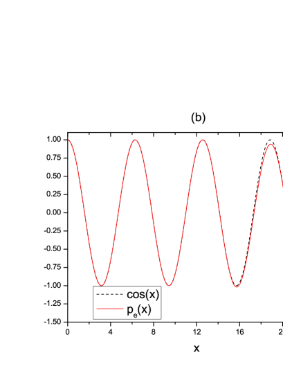
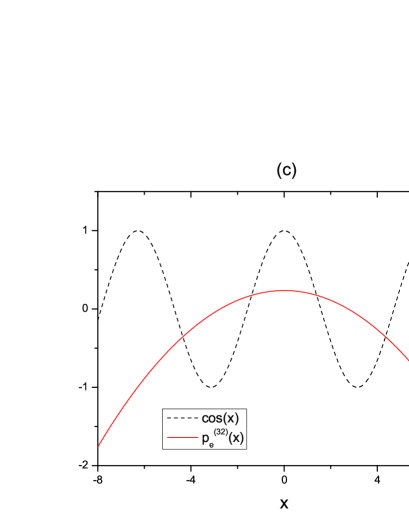
Figure 1: [color online.] (a) The time evolution of root fidelity $\sqrt{F}$ for $|\varphi_{e}(0)\rangle$ under the Hamiltonian $H_{e}$. (b) The polynomial $p_{e}(x)$ is a very good approximation of $\cos x$ for $0\leq x\lesssim 22$. (c) The curves $\cos(x)$ and $p_{e}^{(32)}(x)$ intersect at four distinct points only. (d) A plot of the R.H.S. of inequality (3b) with $p(x)=p_{e}(x)$ and $\langle|E|^{2k}\rangle=4\hbar^{2k}[1+(11/5)^{2k}]/15$ for $k=1,2,\ldots,17$.

Actually, this method can be adapted to show $p(x)\leq\cos(x-\theta)$ for all $x\geq 0$ for a variety of polynomial $p(x)$ constructed out of Hermite interpolation.

III.3 QSL and a first-order phase transition

Since $p_{e}(x)\leq\cos x$ for all $x\geq 0$, it induces the following QSL:

$$\sqrt{F} \leq 1-5.0000\times 10^{-1}\langle|E|^{2}\rangle\left(\frac{\tau}{\hbar}\right)^{2}+4.1667\times 10^{-2}\langle|E|^{4}\rangle\left(\frac{\tau}{\hbar}\right)^{4}-1.3889\times 10^{-3}\langle|E|^{6}\rangle\left(\frac{\tau}{\hbar}\right)^{6}$$

$$\quad+2.4802\times 10^{-5}\langle|E|^{8}\rangle\left(\frac{\tau}{\hbar}\right)^{8}-2.7557\times 10^{-7}\langle|E|^{10}\rangle\left(\frac{\tau}{\hbar}\right)^{10}+2.0876\times 10^{-9}\langle|E|^{12}\rangle\left(\frac{\tau}{\hbar}\right)^{12}$$

$$\quad-1.1469\times 10^{-11}\langle|E|^{14}\rangle\left(\frac{\tau}{\hbar}\right)^{14}+4.7766\times 10^{-14}\langle|E|^{16}\rangle\left(\frac{\tau}{\hbar}\right)^{16}-1.5585\times 10^{-16}\langle|E|^{18}\rangle\left(\frac{\tau}{\hbar}\right)^{18}$$

$$\quad+4.0798\times 10^{-19}\langle|E|^{20}\rangle\left(\frac{\tau}{\hbar}\right)^{20}-8.6954\times 10^{-22}\langle|E|^{22}\rangle\left(\frac{\tau}{\hbar}\right)^{22}+1.5125\times 10^{-24}\langle|E|^{24}\rangle\left(\frac{\tau}{\hbar}\right)^{24}$$

$$\quad-2.1160\times 10^{-27}\langle|E|^{26}\rangle\left(\frac{\tau}{\hbar}\right)^{26}+2.2929\times 10^{-30}\langle|E|^{28}\rangle\left(\frac{\tau}{\hbar}\right)^{28}-1.7955\times 10^{-33}\langle|E|^{30}\rangle\left(\frac{\tau}{\hbar}\right)^{30}$$

$$\quad+8.9531\times 10^{-37}\langle|E|^{32}\rangle\left(\frac{\tau}{\hbar}\right)^{32}-2.1140\times 10^{-40}\langle|E|^{34}\rangle\left(\frac{\tau}{\hbar}\right)^{34}.$$ (4)

In particular, by putting $\langle|E|^{2k}\rangle=\langle E^{2k}\rangle=4\hbar^{2k}[1+(11/5)^{2k}]/15$ for $k=1,2,\ldots,17$, this construction leads to a QSL which gives a tight lower bound for the evolution time in the cases of $\sqrt{F}=\sqrt{F_{c1}}$ and $\sqrt{F_{c2}}$. Fig. 1d depicts that for root fidelity $\sqrt{F}=\sqrt{F_{c1}}=0$, the corresponding QSL is $\tau\in[\tau_{c1},10.138]\cup[10.248,+\infty)$. Combined with the example of the evolution of $|\varphi_{e}(0)\rangle$, I conclude that whenever a quantum state with $\langle|E|^{2k}\rangle$ is equal to the value given in the previous paragraph for $k=1,2,\ldots,17$, the minimum evolution time $\tau_{\min}$ for it to evolve to another state of root fidelity $0$ is $\tau_{c1}$. By gradually increasing $\sqrt{F}$, the allowable region for $\tau$ increases and $\tau_{\min}\leq\tau_{c1}$. Most importantly, by increasing $\sqrt{F}$ to $\sqrt{F_{c2}}\approx 0.0682$, the allowable $\tau$ becomes $\{\tau_{c2}\}\cup[9.519,+\infty)$ with $\tau_{\min}=\tau_{c2}$. That is, a new permissible time interval appears and a genuine forbidden evolution interval $(\tau_{c2},9.519)$ is formed. Besides, $\tau_{\min}$ shows first-order phase transition at $\sqrt{F}=\sqrt{F_{c2}}$. This is the first QSL that captures this type of phase transition. Further significance of this result is reported in Appendix A.

III.4 The reverse problem

Note that the above method to construct a QSL with genuine forbidden speed intervals is generic. In fact, it brings us to the following reverse problem, which has never been studied before. Given an initial state, an Hamiltonian and a required fidelity $F$, is it possible to find a QSL whose minimum permissible evolution time equals the actual evolution time needed? By modifying the proof of the existence of $p(x)$, I show in Appendix B that the answer is affirmative in finite-dimensional Hilbert space.

IV Discussions and outlook

To summarize, I have reported an efficient method to construct new QSLs. An important feature of this method is that by specifying a finite number of compatible observables in the form of various moments of energy of the system, the resultant QSL is independent of the Hilbert space dimension. Thus, the two most important consequences of this construction, namely, the existence of forbidden speed intervals and certain first-order phase transition are very strong results since they cannot come from an overly restricted set of constraints on a low-dimensional quantum system that almost fixing the Hamiltonian and the initial state. More importantly, this study opens up a more general research direction on the tradeoff between the amount of partial information describing a quantum system and the constraints on its information processing capability in which a lot of works can be done.

Appendix A Further Significance Of The QSL Associated With The Degree 34 Polynomial $\boldsymbol{p_{e}(x)}$ Reported In The Main Text

Recall that for fidelity $F=0$, the QSL reported in inequality (4) in the main text leads to a minimum evolution time of $\tau_{c1}$ for $\langle|E|^{2k}\rangle=4\hbar^{2k}[1+(11/5)^{2k}]/15$ for $k=1,2,\ldots,17$. Further, this bound is tight for it can be achieved by the state $|\varphi_{e}(0)\rangle$ under the evolution of the Hamiltonian $H_{e}$. Note that the highest and lowest energy eigenvector components of $|\varphi_{e}(0)\rangle$ are $|\pm 11\hbar/5\rangle$. Hence, the phase angle difference $\chi$ rotated during the time $\tau_{c1}$ between these two components equals $22\tau_{c1}/5>2\pi$. That is, the relative phase angle between two components has to rotate more than one complete circle in order to evolve $|\varphi_{e}(0)\rangle$ to its orthogonal complement. This is a new situation for these relative phase angles rotated in all known QSLs to date Margolus and Levitin (1996, 1998); Giovannetti et al. (2003); Zieliński and Zych (2006); Chau (2010); Lee and Chau (2013) are at most $2\pi$. The implication is that for states obeying the above constraints on its various moments of energy, they cannot evolve to their orthogonal complement without some time of “time wastage” as some of the relative phase angle change must be greater than a complete circle.

I also remark that this is the first tight QSL with the property that the “magic state” saturating this QSL in the case of $F=0$ has to be at least four-dimensional. The corresponding “magic states” for all previous QSLs are at most three-dimensional Margolus and Levitin (1996, 1998); Giovannetti et al. (2003); Zieliński and Zych (2006); Chau (2010); Lee and Chau (2013). The reason why the “magic state” saturating this QSL is at least four-dimensional is as follows. From the discussion on the conditions for equality of inequality (3b) in the main text and the construction of $p_{e}$ that leads to the QSL, the magic state $|\psi(0)\rangle$, expressed in the energy eigenbasis, must be in the form $\alpha_{0}|0\rangle+\alpha_{1}|E\rangle+\alpha_{2}|-E\rangle+\alpha_{3}|11E/5\rangle+\alpha_{4}|-11E/5\rangle$ with $E>0$. Furthermore, the evolution time to an orthogonal state equals $\tau_{c1}\hbar/E$. For the given constraints in $\langle|E|^{2k}\rangle$’s, I arrive at $|\alpha_{0}|^{2}=7/15$, $|\alpha_{1}|^{2}+|\alpha_{2}|^{2}=|\alpha_{3}|^{2}+|\alpha_{4}|^{2}=4/15$. Consider the imaginary part of $\langle\psi(0)|\psi(\tau_{c1}\hbar/E)\rangle$, I have $(|\alpha_{2}|^{2}-|\alpha_{1}|^{2})\sin\tau_{c1}+(|\alpha_{4}|^{2}-|\alpha_{3}|^{2})\sin(11\tau_{c1}/5)=0$. Hence, at most one of the $\alpha_{j}$’s can be zero. Thus, the “magic state” is at least four-dimensional.

Appendix B Existence Of A QSL For The Reverse Problem For Finite-Dimensional Hilbert Space Systems

Denote the state at time $\tau$ under the evolution of the time-independent Hamiltonian $H$ in a $d$-dimensional Hilbert space by $|\varphi(\tau)\rangle$ with $|\varphi(0)\rangle=\sum_{j=1}^{d}\alpha_{j}|E_{j}\rangle$. Surely, the root fidelity at time $\tau$ is given by the continuous function

$$\sqrt{F}(\tau)=\left|\langle\varphi(0)|\varphi(\tau)\rangle\right|=\sum_{j=1}^{d}|\alpha_{j}|^{2}\cos\left[\frac{E_{j}\tau}{\hbar}-\theta(\tau)\right]$$

where $\theta(\tau)$ is the argument of the complex number $\langle\varphi(0)|\varphi(\tau)\rangle$. Although $\theta$ can only be determined modulo $2\pi$, I may uniquely fix it by the integral curve describing the time evolution of the argument of $\langle\varphi(0)|\varphi(\tau)\rangle$ with initial condition $\theta(0)=0$ provided that $\tau$ is less than or equal to the first time when $\sqrt{F}=0$. And from now on, I assume $\theta(\tau)$ to be this smooth integral curve.

I first write down several properties of the function $\sqrt{F}(\tau)$. Denote the first time when $\sqrt{F}(\tau)$ reaches a certain fixed value $\sqrt{F_{0}}\in[0,1]$ by $\tau_{\min}$. Suppose further that $\tau_{\min}$ is finite. I define $\tau_{\text{turn}}$ and $\epsilon_{0}$ as follows. Suppose $\sqrt{F}(\tau)$ is a decreasing function in $[0,\tau_{\min}]$, then I set $\tau_{\text{turn}}=0$ and $\epsilon_{0}=1$. Otherwise, since $\sqrt{F}$ is continuous and differentiable provided that $\sqrt{F}>0$, there is a turning point in $[0,\tau_{\min})$. Denote the turning point in $[0,\tau_{\min})$ closest to $\tau_{\min}$ by $\tau_{\text{turn}}$. Then, I set $\epsilon_{0}=\min_{\tau\in[0,\tau_{\text{turn}}]}\sqrt{F}(\tau)-\sqrt{F_{0}}$. It is well-defined because the minimum exists owning to the continuity of $\sqrt{F}$; and it is positive for otherwise $\tau_{\min}$ will not be the first time when the root fidelity reaches $\sqrt{F_{0}}$. Note that no matter whether there is a turning point for $\sqrt{F}$ in $[0,\tau_{\min}]$ or not, $\sqrt{F}(\tau)$ is decreasing in $[\tau_{\text{turn}},\tau_{\min}]$. More importantly, for $0\leq\tau\leq\tau_{\min}$, $\sqrt{F}(\tau)<\sqrt{F_{0}}+\epsilon_{0}$ only in $[\tau_{\text{turn}},\tau_{\min}]$. That is to say, the function $\sqrt{F}(\tau)$ is one-one in the domain $[\tau_{\text{turn}^{\prime}},\tau_{\min}]$ and range $[\sqrt{F_{0}},\sqrt{F_{0}}+\epsilon_{0}]$, where $\tau_{\text{turn}^{\prime}}$ is the closest point to $\tau_{\min}$ in $[0,\tau_{\min})$ with $\sqrt{F}(\tau_{\text{turn}^{\prime}})=\sqrt{F_{0}}+\epsilon_{0}$. Last but not least, for a sufficiently small $\delta>0$,

$$\sqrt{F}(\tau)-\sqrt{F_{0}}=\mbox{O}((\tau_{\min}-\tau)^{\beta})$$

for $\tau\in(\tau_{\min}-\delta,\tau_{\min})$ for some $\beta>0$.

Next, I consider the QSL induced by a polynomial $p(x)$. Using the idea in the main text, suppose $\cos x\geq p(x)=\sum_{k=0}^{n}c_{k}x^{k}$ for all $x\geq x_{\min}\equiv\min_{j}\min_{\tau\in[0,\tau_{\min}]}[E_{j}\tau/\hbar-\theta(\tau)]$. Then, I have a QSL in the form of an inequality

$$\sqrt{F}(\tau) \geq\sum_{j=1}^{d}|\alpha_{j}|^{2}p(\frac{E_{j}\tau}{\hbar}-\theta(\tau))$$

$$=\sum_{j=1}^{d}\sum_{k=0}^{n}c_{k}|\alpha_{j}|^{2}\left[\frac{E_{j}\tau}{\hbar}-\theta(\tau)\right]^{k}$$

$$=\sum_{k=0}^{n}\sum_{\ell=0}^{k}c_{k}\binom{k}{\ell}\langle E^{\ell}\rangle\theta(\tau)^{k-\ell}\left(\frac{\tau}{\hbar}\right)^{\ell}$$ (5)

whenever $0\leq\tau\leq\tau_{\min}$.

Now, I consider the set of polynomials ${\mathcal{S}}_{n,\gamma}$ with the properties that $p(x)\in{\mathcal{S}}_{n,\gamma}$ if and only if

• $\deg p(x)\leq n$;

• $p(x)\leq\cos x$ whenever $x\geq x_{\min}$;

• $p(x_{j})=\cos x_{j}$ for all $j$, where $x_{j}=E_{j}\tau_{\min}/\hbar-\theta(\tau_{\min})$; and

• $\cos x-p(x)=\mbox{O}((x-x_{j})^{\gamma})$ in the neighborhood of $x_{j}$ for all $j$.

Using the Hermite interpolating polynomial construction in the main text, I know that for each fixed $\gamma>1$, the set ${\mathcal{S}}_{n,\gamma}$ is non-empty provided that $n$ is sufficiently large. Clearly, ${\mathcal{S}}_{n,\gamma}$ is a convex set. In addition, it is easy to see that the functional

$$G[f_{1},f_{2}]=\max_{x\in[x_{\min},x_{\max}]}\left|f_{1}(x)-f_{2}(x)\right|$$

is convex where $x_{\max}=\max_{j}[E_{j}\tau_{\min}/\hbar-\theta(\tau_{\min})]$.

Note that for a fixed $\gamma>1$, there is a sequence of polynomials $p_{n}(x)\in{\mathcal{S}}_{n,\gamma}$ such that $\lim_{n\to+\infty}G[p_{n}(x),\cos x]=0$. In fact, each $p_{n}(x)$ can be chosen to be the optimal degree $\leq n$ polynomial in ${\mathcal{S}}_{n,\gamma}$ that minimizes the functional $G[\cos x,\cdot]$ via convex optimization Boyd and Vandenberghe (2004).

With the above background preparation, I am ready to prove the existence of a polynomial $p(x)$ that solves the reverse problem. That is, the QSL induced by $p(x)$ in inequality (5) has the property that the smallest non-negative time at which the R.H.S. of this inequality is $\sqrt{F_{0}}$ occurs when $\tau=\tau_{\min}$ provided that $\langle E^{k}\rangle$’s are set to the $k$th moment of the energy of the state $|\varphi(0)\rangle$.

I choose a sufficiently small $0<\delta<\tau_{\min}-\tau_{\text{turn}}$ such that

$$\sqrt{F}(\tau)-\sqrt{F_{0}}\geq\zeta(\tau_{\min}-\tau)^{\beta}$$

for all $\tau\in(\tau_{\min}-\delta,\tau_{\min}]$, where $\zeta>0$. For this $\delta>0$, I can find sufficiently large $\gamma$ and $n$ such that ${\mathcal{S}}_{n,\gamma}$ is non-empty and the $p(x)\in{\mathcal{S}}_{n,\gamma}$ that minimizes the functional $G[\cos x,\cdot]$ obeys $G[\cos x,p(x)]<\epsilon$ where

$$\epsilon\equiv\sqrt{F}(\tau_{\min}-\delta)-\sqrt{F_{0}}\in(0,\epsilon_{0}].$$

I claim that the QSL induced by this $p(x)$ solves the reverse problem. This is because by my construction, for $\tau=\tau_{\min}$, the R.H.S. of inequality (5) equals $\sum_{j}|\alpha_{j}|^{2}p(x_{j})=\sum_{j}|\alpha_{j}|^{2}\cos x_{j}=\sqrt{F_{0}}=\sqrt{F}(\tau_{\min})$.

I proceed to consider the case of $\tau\in[0,\tau_{\min}-\delta]$. As $\cos x-p(x)\leq G[\cos x,p(x)]<\epsilon$ for all $x>x_{\min}$, I conclude that

$$\sqrt{F}(\tau) =\sum_{j}|\alpha_{j}|^{2}\cos\left[\frac{E_{j}\tau}{\hbar}-\theta(\tau)\right]$$

$$<\epsilon+\sum_{j}|\alpha_{j}|^{2}p(\frac{E_{j}\tau}{\hbar}-\theta(\tau)).$$

Hence,

$$\sum_{j}|\alpha_{j}|^{2}p(\frac{E_{j}\tau}{\hbar}-\theta(\tau)) >\sqrt{F}(\tau)-\epsilon$$

$$\geq\sqrt{F}(\tau_{\min}-\delta)-\epsilon$$

$$=\sqrt{F_{0}}.$$

In other words, the R.H.S. of inequality (5) greater than $\sqrt{F_{0}}$ in the time interval $[0,\tau_{\min}-\delta]$.

Finally, I consider the case of $\tau\in(\tau_{\min}-\delta,\tau_{\min})$. I have

$$\sqrt{F_{0}}+\zeta(\tau_{\min}-\tau)^{\beta}$$

$$\leq \sqrt{F}(\tau)$$

$$= \sum_{j}|\alpha_{j}|^{2}p(\frac{E_{j}\tau}{\hbar}-\theta(\tau))+\mbox{O}((\Delta_{j}(\tau))^{\gamma})$$

where $\Delta_{j}(\tau)=E_{j}(\tau_{\min}-\tau)/\hbar+\theta(\tau)-\theta(\tau_{\min})$. Since $\theta(\tau)$ is smooth in this time interval, $\Delta_{j}(\tau)=\mbox{O}((\tau_{\min}-\tau)^{\gamma^{\prime}})$ for some $\gamma^{\prime}>0$. Therefore,

$$\sum_{j}|\alpha_{j}|^{2}p(\frac{E_{j}\tau}{\hbar}-\theta(\tau))$$

$$\geq \sqrt{F_{0}}+\zeta(\tau_{\min}-\tau)^{\beta}+\mbox{O}((\tau_{\min}-\tau)^{\gamma\gamma^{\prime}}).$$

Since $\zeta>0$, by picking a sufficiently small $\delta>0$ and a sufficiently large $\gamma$ so that $\gamma\gamma^{\prime}>\beta$ (and a sufficient large $n$ so that ${\mathcal{S}}_{n,\gamma}$ is non-empty), the R.H.S. of inequality (5) is greater than $\sqrt{F_{0}}$ in this time interval.

To summarize, the QSL induced by any $p(x)$ in this ${\mathcal{S}}_{n,\beta}$ is a solution of the reverse problem. This completes the proof of my claim.

Lastly, let me make the following remark. Suppose $0\leq\tau_{1}<\tau_{2}<\ldots<\tau_{\ell}$ are $\ell$ distinct numbers with $\sqrt{F}(\tau_{j})=\sqrt{F_{0}}$ for all $j$, where $\sqrt{F}(\tau)$ is the root fidelity between $|\varphi(\tau)\rangle$ and $|\varphi(0)\rangle$ under the action of a time-independent Hamiltonian $H$. Then, it is not difficult to adapt the above procedure to construct a polynomial whose induced QSL has the properties that

• the induced QSL is an equality at times $\tau_{1},\ldots,\tau_{\ell}$ provided that $\sqrt{F}=\sqrt{F_{0}}$ and $\langle E^{k}\rangle$ is the $k$th moment of the average energy of the state $|\varphi(0)\rangle$;

• the induced QSL is a strict inequality at time $\tau\in[0,\tau_{\ell}]$ provided that $\sqrt{F}(\tau)>F_{0}$.

The proof is left to the interested readers.

References

- Lloyd (2000) S. Lloyd, Nature 406, 1047 (2000).
- Margolus and Levitin (1996) N. Margolus and L. B. Levitin, in Proceedings of the 4th workshop on physics and computation (PHYSCOMP 96), edited by T. Toffoli, M. Biafore, and J. Leaõ (New England Complex Systems Institute, Cambridge, MA, 1996) p. 208.
- Margolus and Levitin (1998) N. Margolus and L. B. Levitin, Physica D 120, 188 (1998).
- Giovannetti et al. (2003) V. Giovannetti, S. Lloyd, and L. Maccone, Phys. Rev. A 67, 052109 (2003).
- Mandelstam and Tamm (1945) L. Mandelstam and I. Tamm, J. Phys. (USSR) 9, 249 (1945).
- Fleming (1973) G. N. Fleming, Nuovo Cimento A 16, 232 (1973).
- Bhattacharyya (1983) K. Bhattacharyya, J. Phys. A 16, 2993 (1983).
- Uhlmann (1992) A. Uhlmann, Phys. Lett. A 161, 329 (1992).
- Pfeifer (1993) P. Pfeifer, Phys. Rev. Lett. 70, 3365 (1993), and erratum in Phys. Rev. Lett. 70, 306 (1993).
- Zieliński and Zych (2006) B. Zieliński and M. Zych, Phys. Rev. A 74, 034301 (2006).
- Jones and Kok (2010) P. J. Jones and P. Kok, Phys. Rev. A 82, 022107 (2010).
- Chau (2010) H. F. Chau, Phys. Rev. A 81, 062133 (2010).
- Lee and Chau (2013) K. Y. Lee and H. F. Chau, J. Phys. A 46, 015305 (2013).
- Levitin and Toffoli (2009) L. B. Levitin and T. Toffoli, Phys. Rev. Lett. 103, 160502 (2009).
- Stoer and Bulirsch (2002) J. Stoer and R. Bulirsch, Introduction to numerical analysis, 3rd ed. (Springer, Berlin, 2002) §2.1.5.
- McNamee (2007) J. M. McNamee, Numerical methods for roots of polynomials. Part I (Elsevier, Amsterdam, 2007).
- Alefeld and Herzberger (1983) G. Alefeld and J. Herzberger, Introduction to interval computations, 2nd ed. (Academic Press, New York, 1983).
- Pan (1997) V. Y. Pan, SIAM Rev. 39, 187 (1997).
- Uhlmann (1995) A. Uhlmann, Rep. Math. Phys. 36, 461 (1995).
- Boyd and Vandenberghe (2004) S. Boyd and L. Vandenberghe, Convex optimization (CUP, Cambridge, U.K., 2004).