On Infectious Model for Dependent Defaults

Abstract

In this paper, we propose a two-sector Markovian infectious model, which is an extension of Greenwood’s model. The central idea of this model is that the causality of defaults of two sectors is in both direction, which enrich dependence dynamics. The Bayesian Information Criterion is adopted to compare the proposed model with the two-sector model in credit literature using the real data. We find that the newly proposed model is statistically better than the model in past literature. We also introduce two measures: CRES and CRVaR to give risk evaluation of our model.

Keywords: Contagion Model, Markov Chain, Two-sector Model, Risk Management, Causality.

1 Introduction

Modeling dependent default risk has been a key issue in credit risk modeling. There are two important approaches to model the dependent default risk. The structural firm model has its origin in Merton (1974) and Black and Scholes (1973), which models the relationship between the firm’s asset value and the defaults. The reduced-form intensity-based model by Jarrow and Turnbull (1995) use Poisson jump processes to model the default event.

Copula has been a very popular tool in modeling the dependent risk. The idea of Copula is transforming the marginal variables to uniform variables by a simple transformation. After this is done, a n-dimensional function is used to model the dependence of the uniform variables, which is so called the Copula function. The Copula helps us to deal with the multivariate distribution of the uniform variable, without consideration of the original marginal variables. There are many useful Copulas in finance. The Gaussian Copula, which is introduced by Li (2000), is widely used in risk modeling and financial assessment.

In addition, conditional independence model is also a commonly used model in credit risk modeling. Conditional on the systematical common factor, the loss random variables are independent. To specify, the Bernoulli mixture model is followed by the $CreditMetrics$ and $KMV$-model, while the Poisson mixture model is followed by the $CreditRisk^{+}$ model. In a recession, the default of one company is triggered by the underlying common risk factor and also by the related company’s defaults. The contagion model is used to describe how the credit event of one company affects the other companies. Davis and Lo (2001) introduce an infectious default model, where in a portfolio a bond may be infected by defaults of other bonds or default directly. Jarrow and Yu (2001) propose a reduced-form model to describe the defaultable bonds of different company, where the concept of counterparty risk is first introduced to the credit literature.

Ching et al. (2008) introduce an infectious default model based on the idea of Greenwood’s model considered in Daley and Gani (1999) . This model aims at modeling the impact of default of a bond on the likelihood of defaults of other bonds. The original version of Greenwood’s model is a one-sector model. It is then extended to a two-sector model in Ching et al. (2008). Besides, the joint probability distribution function for the duration of a default crisis, (ie, the default cycle), and the severity of defaults during the crisis period was also derived. Two concepts, namely, the Crisis Value-at-Risk (CRVaR) and the Crisis Expected Shortfall (CRES), are also used to assess the impact of a default crisis. The Greenwood’s model is also extended to a network of sectors in Ching et al. (2010). Gu et al. (2011) propose a Markovian infectious model to describe the dependent relationship of default processes of credit securities based on Ching et al. (2008, 2010), where the central idea is the concept of common shocks which is one of the major approaches to describe insurance risk.

In this paper, we propose a two-sector Markovian infectious model, where the future default probability switching over time depends on the current number of defaults of both sectors. Moreover, the defaults of sector A caused by th defaults of sector B, and vice versa. The causality of defaults in both direction is captured by the underlying switched default probability. We adopt the maximum likelihood method to estimate the parameters and the Bayesian Information Criterion to compare the propose model with two-sector model considered in Ching et al. (2008). The experiment result shows that the proposed model outperforms the model in credit literature. In addition, a more general model is given to provide more flexibility in describing realistic features of the dynamics of default probabilities.

This paper is structured as follows. Section 2 presents our proposed model. And we also derive a recursive formula for the joint probability distribution for the default cycle and the number of defaults during the crisis and outline the estimation procedure. Section 3 presents the ideas of the CRVaR and the CRES. In Section 4, we present the results of empirical analysis using our proposed model. Section 5 gives the general model extending the proposed model in Section 2. The final section concludes the paper.

2 The Basic Model

Let ${\cal T}$ be the time index set $\{0,1,2,\ldots,\}$ of our model. To model the uncertainty, we consider a probability space $(\Omega,{\cal F},{\cal P})$, where ${\cal P}$ is a real-world probability. Suppose that

$$X:=\{{X_{t}}\}_{t\in{\cal T}}\quad{\rm and}\quad Y:=\{{Y_{t}}\}_{t\in{\cal T}}$$

denote two stochastic processes on $(\Omega,{\cal F},{\cal P})$, where $X_{t}=({X^{1}_{t}},{X^{2}_{t}})$ and $Y_{t}=({Y^{1}_{t}},{Y^{2}_{t}})$ represent the numbers of surviving bonds and the defaulted bonds at $t\in{\cal T}$ in sector A and sector B, respectively, e.g., $X^{1}_{t}$ represents the the number of surviving bonds at time t in sector A. We assume that the initial conditions are given as follows:

$$X_{0}=(x^{1}_{0},x^{2}_{0}),\quad Y_{0}=(y^{1}_{0},y^{2}_{0})\quad{\rm and}\quad x^{1}_{0}+y^{1}_{0}=N_{1},\quad x^{2}_{0}+y^{2}_{0}=N_{2}\ .$$

Note that for each $t\in{\cal T}$, the sum of the numbers of the defaulted bonds and the surviving bonds at the time epoch $t+1$ must equal the number of surviving bonds at time $t$ in every sector, i.e.,

$$X^{1}_{t+1}+Y^{1}_{t+1}=X^{1}_{t}\quad{\rm and}\quad X^{2}_{t+1}+Y^{2}_{t+1}=X^{2}_{t}.$$ (1)

For each $t\in{\cal T}$, let ${\alpha}_{t}$ and ${\beta}_{t}$ be the probability that the default of a surviving bond is infected by the defaulted bonds at time $t$ in sector A and sector B, respectively. The joint probability distribution of $\{X_{t+1},Y_{t+1}\}$ given $\{X_{t},Y_{t}\}$ is given by the following Binomial probability:

$$\begin{array}[]{lll}p_{(x_{t},y_{t})}(x_{t+1},y_{t+1})&=&P\{(X_{t+1},Y_{t+1})=(x_{t+1},y_{t+1})\mid(X_{t},Y_{t})=(x_{t},y_{t})\}\\ &=&\left(\begin{array}[]{c}x^{1}_{t}\\ y^{1}_{t+1}\end{array}\right){(\alpha}_{t})^{y^{1}_{t+1}}(1-{\alpha}_{t})^{x^{1}_{t+1}}\times\left(\begin{array}[]{c}x^{2}_{t}\\ y^{2}_{t+1}\end{array}\right){(\beta}_{t})^{y^{2}_{t+1}}(1-{\beta}_{t})^{x^{2}_{t+1}}.\\ \end{array}$$ (8)

We consider here the situation that the joint future default probability depends on the current number of defaulted bonds of both industrial sectors. We assume that

$$\begin{array}[]{llll}{\alpha}_{t}&=&a(y_{t})\\ &=&\left\{\begin{array}[]{llll}a_{0}&{\rm if}&y^{1}_{t}=y^{2}_{t}=0\\ a_{1}&{\rm if}&y^{1}_{t}>0,y^{2}_{t}=0\\ a_{2}&{\rm if}&y^{1}_{t}=0,y^{2}_{t}>0\\ a_{3}&{\rm if}&y^{1}_{t}>0,y^{2}_{t}>0\end{array}\right.\\ &=&a_{0}h_{0}(y^{1}_{t},y^{2}_{t})+a_{1}h_{1}(y^{1}_{t},y^{2}_{t})+a_{2}h_{2}(y^{1}_{t},y^{2}_{t})+a_{3}h_{3}(y^{1}_{t},y^{2}_{t})\end{array}$$ (16)

and

$$\begin{array}[]{lll}{\beta}_{t}&=&b(y_{t})\\ &=&\left\{\begin{array}[]{llll}b_{0}&{\rm if}&y^{1}_{t}=y^{2}_{t}=0\\ b_{1}&{\rm if}&y^{1}_{t}=0,y^{2}_{t}>0\\ b_{2}&{\rm if}&y^{1}_{t}>0,y^{2}_{t}=0\\ b_{3}&{\rm if}&y^{1}_{t}>0,y^{2}_{t}>0\end{array}\right.\\ &=&b_{0}h_{0}(y^{2}_{t},y^{1}_{t})+b_{1}h_{1}(y^{2}_{t},y^{1}_{t})+b_{2}h_{2}(y^{2}_{t},y^{1}_{t})+b_{3}h_{3}(y^{2}_{t},y^{1}_{t}),\end{array}$$ (24)

where

$$h_{0}(x,y)=\left\{\begin{array}[]{ll}1&{\rm if}\ x=y=0\\ 0&{\rm otherwise}\end{array}\right.,\quad h_{1}(x,y)=\left\{\begin{array}[]{ll}1&{\rm if}\ x>0,y=0\\ 0&{\rm otherwise}\end{array}\right.$$

and

$$h_{2}(x,y)=\left\{\begin{array}[]{ll}1&{\rm if}\ x=0,y>0\\ 0&{\rm otherwise}\end{array}\right.,\quad h_{3}(x,y)=\left\{\begin{array}[]{ll}1&{\rm if}\ x>0,y>0\\ 0&{\rm otherwise}.\end{array}\right.$$

As it is shown in Equation (1)(8), one can see that $\{X_{t},t=0,1,2,\ldots\}$ is a second-order Markov chain process. We remark that this two-sector model provides a novel and flexible dependent structure for correlated defaults of two different industrial sectors. Firstly, an infectious default within one time period is modeled as a Binomial distribution, which has been widely used in modeling the spread of epidemics whose situation is quite similar to that of a financial crisis. The causality of the infection is supposed to be in both direction, i.e., a “looping default”. Secondly, the process $(X_{t},Y_{t})$ has the Markov property, where the probabistic structure of future states only depend on the current state. Thirdly, conditioning on the current state $(X_{t},Y_{t})$, the future state of two sectors $(X^{1}_{t+1},Y^{1}_{t+1})$ and $(X^{2}_{t+1},Y^{2}_{t+1})$ are stochastically independent. The step functions $h_{i}(x,y)$ are used to describe the dependence of the default probabilities on the state of previous time epoch. On one hand, this method provides a tractable and analytic solution for parameter estimation from empirical data. On the other hand, one has to admit that this simplicity may result in limitations in applications. In Section 5, we relax the assumption of the specific form for $\alpha_{t}$ and $\beta_{t}$ and a more complicated dependent structure modelling framework is presented.

2.1 Default Cycle and Severity

In this subsection, we proceed to derive the joint probability distribution function (p.d.f) for the duration of the default crisis ($T$), namely, the default cycle, and the severity of the defaults ($W_{T}$) during the crisis period. These two concepts are essential in determining the impact of a default crisis. We first give a precise definition of the default cycle:

$$T:={\rm inf}\{t\in{\cal T}\mid Y_{t}=0\}.$$ (25)

And given $T=t>0$, $W_{t}$ represents the number of defaults in the sector over the time duration $(0,t]$. To apply the concepts of default cycle and the severity of the defaults on our proposed two-sector model, we write

$$T_{1}:={\rm inf}\{t\in{\cal T}\mid Y^{1}_{t}=0\}\quad{\rm and}\quad T_{2}:={\rm inf}\{t\in{\cal T}\mid Y^{2}_{t}=0\}.$$

Provided that $T_{1}=t_{1}>0$ and $T_{2}=t_{2}>0$, $W^{1}_{t_{1}}$ and $W^{2}_{t_{2}}$ represent the number of defaults in sector A and sector B respectively in $(0,t_{1}]$ and $(0,t_{2}]$. To obtain the joint distribution of $(W^{i}_{T_{i}},T_{i})$ for $i=1,2$, we assume that $(X_{0},Y_{0})=(x_{0},y_{0})$ with $y^{1}_{0}>0,y^{2}_{0}>0$. Let

$$P_{n}(x_{1},x_{2},h)=P\{T_{1}\geq n+1,X^{1}_{n}=x_{1},X^{2}_{n}=x_{2},I_{\{Y^{2}_{n}>0\}}=h\}.$$

The following Lemma gives recursive formulas for $P_{n}(x_{1},x_{2},h)$.

Lemma 1

$$\begin{array}[]{ll}P_{n}(x_{1},x_{2},0)=&\displaystyle\sum_{s_{1}>x_{1}}{s_{1}\choose x_{1}}\left[P_{n-1}(s_{1},x_{2},0)(a_{1})^{s_{1}-x_{1}}(1-a_{1})^{x_{1}}(1-b_{2})^{x_{2}}\right.\\ &\displaystyle\left.+P_{n-1}(s_{1},x_{2},1)(a_{3})^{s_{1}-x_{1}}(1-a_{3})^{x_{1}}(1-b_{3})^{x_{2}}\right]\\ P_{n}(x_{1},x_{2},1)=&\displaystyle\sum_{s_{1}>x_{1}}\sum_{s_{1}>x_{1}}{s_{1}\choose x_{1}}{s_{2}\choose x_{2}}\left[P_{n-1}(s_{1},s_{2},0)(a_{1})^{s_{1}-x_{1}}(1-a_{1})^{x_{1}}(b_{2})^{s_{2}-x_{2}}(1-b_{2})^{x_{2}}\right.\\ &\displaystyle\left.+P_{n-1}(s_{1},s_{2},1)(a_{3})^{s_{1}-x_{1}}(1-a_{3})^{x_{1}}(b_{3})^{s_{2}-x_{2}}(1-b_{3})^{x_{2}}\right]\end{array}$$

where the initial condition is given by

$$P_{0}(x_{1},x_{2},h)=\left\{\begin{array}[]{ll}1,&(x_{1},x_{2},h)=(x^{1}_{0},x^{2}_{0},1)\\ 0,&{\rm otherwise}.\end{array}\right.$$

Proof: By the law of total probability and Markov property,

$$\begin{array}[]{lll}&P_{n}(x_{1},x_{2},0)\\ =&P\{T_{1}\geq n+1,X^{1}_{n}=x_{1},X^{2}_{n}=x_{2},I_{\{Y^{2}_{n}>0\}}=0\}\\ =&{\displaystyle\sum_{s_{1}>x_{1}}\sum_{h=0,1}}P\{T_{1}\geq n,X^{1}_{n-1}=s_{1},X^{2}_{n-1}=x_{2},I_{\{Y^{2}_{n-1}>0\}}=h\}\\ &\times P\{T_{1}\geq n+1,X^{1}_{n}=x_{1},X^{2}_{n}=x_{2},I_{\{Y^{2}_{n}>0\}}=0\mid T_{1}\geq n,X^{1}_{n-1}=s_{1},X^{2}_{n-1}=x_{2},I_{\{Y^{2}_{n-1}>0\}}=h\}\\ =&{\displaystyle\sum_{s_{1}>x_{1}}\sum_{h=0,1}}P_{n-1}(s_{1},x_{2},h)\\ &\times P\{Y^{1}_{n}>0,X^{1}_{n}=x_{1},X^{2}_{n}=x_{2},I_{\{Y^{2}_{n}>0\}}=0\mid T_{1}\geq n,X^{1}_{n-1}=s_{1},X^{2}_{n-1}=x_{2},I_{\{Y^{2}_{n-1}>0\}}=h\}\\ =&{\displaystyle\sum_{s_{1}>x_{1}}\sum_{h=0,1}}P_{n-1}(s_{1},x_{2},h)\\ &\times P\{Y^{1}_{n}>0,X^{1}_{n}=x_{1},X^{2}_{n}=x_{2},I_{\{Y^{2}_{n}>0\}}=0\mid Y^{1}_{n-1}>0,X^{1}_{n-1}=s_{1},X^{2}_{n-1}=x_{2},I_{\{Y^{2}_{n-1}>0\}}=h\}\\ =&{\displaystyle\sum_{s_{1}>x_{1}}}{s_{1}\choose x_{1}}\left[P_{n-1}(s_{1},x_{2},0)(a_{1})^{s_{1}-x_{1}}(1-a_{1})^{x_{1}}(1-b_{2})^{x_{2}}\right.\\ &\displaystyle\left.+P_{n-1}(s_{1},x_{2},1)(a_{3})^{s_{1}-x_{1}}(1-a_{3})^{x_{1}}(1-b_{3})^{x_{2}}\right]\end{array}$$

Similarly, we have

$$\begin{array}[]{lll}&P_{n}(x_{1},x_{2},1)\\ =&P\{T_{1}\geq n+1,X^{1}_{n}=x_{1},X^{2}_{n}=x_{2},I_{\{Y^{2}_{n}>0\}}=1\}\\ =&{\displaystyle\sum_{s_{1}>x_{1}}\sum_{s_{2}>x_{2}}\sum_{h=0,1}}P\{T_{1}\geq n,X^{1}_{n-1}=s_{1},X^{2}_{n-1}=s_{2},I_{\{Y^{2}_{n-1}>0\}}=h\}\\ &\times P\{T_{1}\geq n+1,X^{1}_{n}=x_{1},X^{2}_{n}=x_{2},I_{\{Y^{2}_{n}>0\}}=1\mid T_{1}\geq n,X^{1}_{n-1}=s_{1},X^{2}_{n-1}=s_{2},I_{\{Y^{2}_{n-1}>0\}}=h\}\\ =&{\displaystyle\sum_{s_{1}>x_{1}}\sum_{s_{2}>x_{2}}\sum_{h=0,1}}P_{n-1}(s_{1},s_{2},h)\\ &\times P\{Y^{1}_{n}>0,X^{1}_{n}=x_{1},X^{2}_{n}=x_{2},I_{\{Y^{2}_{n}>0\}}=1\mid T_{1}\geq n,X^{1}_{n-1}=s_{1},X^{2}_{n-1}=s_{2},I_{\{Y^{2}_{n-1}>0\}}=h\}\\ =&{\displaystyle\sum_{s_{1}>x_{1}}\sum_{s_{2}>x_{2}}\sum_{h=0,1}}P_{n-1}(s_{1},s_{2},h)\\ &\times P\{Y^{1}_{n}>0,X^{1}_{n}=x_{1},X^{2}_{n}=x_{2},I_{\{Y^{2}_{n}>0\}}=1\mid Y^{1}_{n-1}>0,X^{1}_{n-1}=s_{1},X^{2}_{n-1}=s_{2},I_{\{Y^{2}_{n-1}>0\}}=h\}\\ =&{\displaystyle\sum_{s_{1}>x_{1}}\sum_{s_{1}>x_{1}}}{s_{1}\choose x_{1}}{s_{2}\choose x_{2}}\left[P_{n-1}(s_{1},s_{2},0)(a_{1})^{s_{1}-x_{1}}(1-a_{1})^{x_{1}}(b_{2})^{s_{2}-x_{2}}(1-b_{2})^{x_{2}}\right.\\ &\displaystyle\left.+P_{n-1}(s_{1},s_{2},1)(a_{3})^{s_{1}-x_{1}}(1-a_{3})^{x_{1}}(b_{3})^{s_{2}-x_{2}}(1-b_{3})^{x_{2}}\right]\end{array}$$

Proposition 1

The joint distribution of $(T_{1},W^{1}_{T_{1}})$ is given by

$$P\{(T_{1},W^{1}_{T_{1}})=(n,x)\}=\sum_{x_{2}}P_{n-1}(x^{1}_{0}-x,x_{2},0)(1-a_{1})^{x^{1}_{0}-x}+\sum_{x_{2}}P_{n-1}(x^{1}_{0}-x,x_{2},1)(1-a_{3})^{x^{1}_{0}-x}.$$

Proof:

$$\begin{array}[]{lll}&P\{(T_{1},W^{1}_{T_{1}})=(n,x)\}\\ =&P\{T_{1}\geq n,Y^{1}_{n}=0,X^{1}_{n}=x^{1}_{0}-x\}\\ =&{\displaystyle\sum_{x_{2}}\sum_{h=0,1}}P\{T_{1}\geq n,X^{1}_{n-1}=x^{1}_{0}-x,X^{2}_{n-1}=x_{2},I_{\{Y^{2}_{n-1}>0\}}=h\}\\ &\times P\{Y^{1}_{n}=0,X^{1}_{n}=x^{1}_{0}-x\mid T_{1}\geq n,X^{1}_{n-1}=x^{1}_{0}-x,X^{2}_{n-1}=x_{2},I_{\{Y^{2}_{n-1}>0\}}=h\}\\ =&{\displaystyle\sum_{x_{2}}\sum_{h=0,1}}P_{n-1}(x^{1}_{0}-x,x_{2},h)\\ &\times P\{Y^{1}_{n}=0,X^{1}_{n}=x^{1}_{0}-x\mid Y^{1}_{n-1}>0,X^{1}_{n-1}=x^{1}_{0}-x,X^{2}_{n-1}=x_{2},I_{\{Y^{2}_{n-1}>0\}}=h\}\\ =&\sum_{x_{2}}P_{n-1}(x^{1}_{0}-x,x_{2},0)(1-a_{1})^{x^{1}_{0}-x}+\sum_{x_{2}}P_{n-1}(x^{1}_{0}-x,x_{2},1)(1-a_{3})^{x^{1}_{0}-x}\end{array}$$

We remark that due to the symmetric property of the two sectors, the joint distribution $(W^{2}_{T_{2}},T_{2})$ shares a similar form of $(W^{1}_{T_{1}},T_{1})$.

2.2 Parameter Estimation

This two-sector model has eight parameters: $a_{0}$, $a_{1}$, $a_{2}$, $a_{3}$ and $b_{0}$, $b_{1}$, $b_{2}$, $b_{3}$. We employ the maximum likelihood method to estimate the parameters. Given the total bonds $N_{1}$, $N_{2}$ and the observations of the number of defaulted bonds $y^{1}_{0},y^{1}_{1},\ldots,y^{1}_{N}$ and $y^{2}_{0},y^{2}_{1},\ldots,y^{2}_{N}$, where $N$ denotes the period of observation time, the number of surviving binds $x^{1}_{0},x^{1}_{1},\ldots,x^{1}_{N}$ and $x^{2}_{0},x^{2}_{1},\ldots,x^{2}_{N}$ are deterministic. The following proposition gives analytical expressions for the maximum likelihood estimates of the model parameters.

Proposition 2

For $i=0,1,2,3$,

$$\hat{a}_{i}=\frac{\sum\limits_{t=0}^{N-1}y^{1}_{t+1}h_{i}(y^{1}_{t},y^{2}_{t})}{\sum\limits_{t=0}^{N-1}x^{1}_{t}h_{i}(y^{1}_{t},y^{2}_{t})}\quad{\rm and}\quad\hat{b}_{i}=\frac{\sum\limits_{t=0}^{N-1}y^{2}_{t+1}h_{i}(y^{2}_{t},y^{1}_{t})}{\sum\limits_{t=0}^{N-1}x^{2}_{t}h_{i}(y^{2}_{t},y^{1}_{t})}.$$

Proof: We prove the expression for $\hat{a}_{0}$ here and the proof for the others are similar. The likelihood function $L(a,b\mid x_{0},x_{1},\ldots,x_{N},y_{0},y_{1},\dots,y_{N})$ is then the joint probability density function $f(x_{0},x_{1},\ldots,x_{N},y_{0},y_{1},\ldots,y_{N}\mid a,b)$:

$$\begin{array}[]{llllll}&&L(a,b\mid x_{0},x_{1},\ldots,x_{N},y_{0},y_{1},\ldots,y_{N})\\ &=&f(x_{0},x_{1},\ldots,x_{N},y_{0},y_{1},\ldots,y_{N}\mid a,b)\\ &=&\left(\begin{array}[]{c}x^{1}_{0}\\ x^{1}_{1}\end{array}\right)(1-a(y_{0}))^{x^{1}_{1}}{a(y_{0})}^{y^{1}_{1}}\times\left(\begin{array}[]{c}x^{2}_{0}\\ x^{2}_{1}\end{array}\right)(1-b(y_{0}))^{x^{2}_{1}}{b(y_{0})}^{y^{2}_{1}}\\ &&\times\left(\begin{array}[]{c}x^{1}_{1}\\ x^{1}_{2}\end{array}\right)(1-a(y_{1}))^{x^{1}_{2}}{a(y_{1})}^{y^{1}_{2}}\times\left(\begin{array}[]{c}x^{2}_{1}\\ x^{2}_{2}\end{array}\right)(1-b(y_{1}))^{x^{2}_{2}}{b(y_{1})}^{y^{2}_{2}}\ldots\ldots\\ &&\times\left(\begin{array}[]{c}x^{1}_{N-1}\\ x^{1}_{N}\end{array}\right)(1-a(y_{N-1}))^{x^{1}_{N}}{a(y_{N-1})}^{y^{1}_{N}}\times\left(\begin{array}[]{c}x^{2}_{N-1}\\ x^{2}_{N}\end{array}\right)(1-b(y_{N-1}))^{x^{2}_{N}}{b(y_{N-1})}^{y^{2}_{N}}.\end{array}$$

Then by solving

$$\frac{\partial\ln L(a,b\mid x_{0},x_{1},\ldots,x_{N},y_{0},y_{1},\ldots,y_{N})}{\partial a_{0}}=0\ ,$$

we have

$$-\sum\limits_{t=0}^{N-1}\frac{x^{1}_{t+1}h_{0}(y^{1}_{t},y^{2}_{t})}{1-a(y_{t})}+\sum\limits_{t=0}^{N-1}\frac{y^{1}_{t+1}h_{0}(y^{1}_{t},y^{2}_{t})}{a(y_{t})}=0.$$

Since for any $t$,

$$\frac{1}{1-a(y_{t})}=\sum\limits_{i=0}^{3}\frac{h_{i}(y^{1}_{t},y^{2}_{t})}{1-a_{i}}\quad{\rm and}\quad\frac{1}{a(y_{t})}=\sum\limits_{i=0}^{3}\frac{h_{i}(y^{1}_{t},y^{2}_{t})}{a_{i}},$$

then

$$\begin{array}[]{lll}0&=&\displaystyle-\sum\limits_{t=0}^{N-1}\sum\limits_{i=0}^{3}\frac{x^{1}_{t+1}h_{0}(y^{1}_{t},y^{2}_{t})h_{i}(y^{1}_{t},y^{2}_{t})}{1-a_{i}}+\sum\limits_{t=0}^{N-1}\sum\limits_{i=0}^{3}\frac{y^{1}_{t+1}h_{0}(y^{1}_{t},y^{2}_{t})h_{i}(y^{1}_{t},y^{2}_{t})}{a_{i}}\\ &=&\displaystyle-\sum\limits_{t=0}^{N-1}\frac{x^{1}_{t+1}h_{0}(y^{1}_{t},y^{2}_{t})}{1-a_{0}}+\sum\limits_{t=0}^{N-1}\frac{y^{1}_{t+1}h_{0}(y^{1}_{t},y^{2}_{t})}{a_{0}}.\end{array}$$

Thus,

$$\hat{a}_{0}=\frac{\sum\limits_{t=0}^{N-1}y^{1}_{t+1}h_{0}(y^{1}_{t},y^{2}_{t})}{\sum\limits_{t=0}^{N-1}x^{1}_{t}h_{0}(y^{1}_{t},y^{2}_{t})}$$

3 Crisis VaR and Crisis ES

In this section, we give a brief introduction to the concepts of the CRVaR and the CRES in Ching et al. (2010). Then we present the evaluation of the CRVaR and the CRES using the proposed models. The CRVaR and the CRES are measures for the duration and the severity of a default crisis. Let

$$L(\cdot,\cdot)(\omega):{\cal T}\times{\cal R}\times\Omega\rightarrow{\cal R}$$

be a real-valued function $L(T,W_{T})(\omega)$ of $T$ and $W_{T}$. We then suppose that for a fixed $\omega\in\Omega$,

$$T(\omega)=t,\quad W_{t}(\omega)=w,\quad{\rm and}\quad L(t,w)(\omega)=l(t,w)\in{\cal R}.$$

That is, the loss from the default crisis is $l(t,w)$ when the duration of default crisis $T=t$ and the number of defaulted bonds in the crisis $W_{t}=w$. We write ${\cal L}(T,W_{T})$ for the space of all loss functions $L(T,W_{T})(\omega)$ generated by $T$ and $W_{T}$.

The CRVaR with probability level $\beta$ under ${\cal P}$ is then defined as a functional $V_{\beta}(\cdot):{\cal L}(T,W_{T})\rightarrow{\cal R}$ such that for each $L(T,W_{T})\in{\cal L}(T,W_{T})$,

$$V_{\beta}(L(T,W_{T})):=\inf\{l\in{\cal R}|{\cal P}(L(T,W_{T})>l)\leq\beta\}\ .$$ (26)

In the language of statistics, $V_{\beta}(L(T,W_{T}))$ is the generalized $\beta$-quantile of the distribution of the loss variable $L(T,W_{T})$ under ${\cal P}$. Since the loss from the default crisis $L(T,W_{T})$ is completely determined when $T$ and $W_{T}$ are given, ${\cal P}(L(T,W_{T})>l)$ is completely determined by the joint p.d.f. of $W_{T}$ and $T$.

The CRES with probability level $\beta$ under ${\cal P}$ is also defined as a functional $E_{\beta}(\cdot):{\cal L}(T,W_{T})\rightarrow{\cal R}$ such that for each $L(T,W_{T})\in{\cal L}(T,W_{T})$,

$$E_{\beta}(L(T,W_{T})):=E_{\cal P}[L(T,W_{T})|L(T,W_{T})\geq V_{\beta}(L(T,W_{T}))].$$ (27)

In other words, $E_{\beta}(L(T,W_{T}))$ is the average of the loss from the default crisis when the loss exceeds the CRVaR of the default crisis with probability level $\beta$ under ${\cal P}$.

4 Empirical Results for Proposed Model

In this section we present the empirical results of the proposed two-sector model using real default data extracted from the figures in Giampieri et al. (2005), where we adopt the estimation methods and techniques presented in the previous section.

The default data comes from four different sectors. They include consumer/service sector, energy and natural resources sector, leisure time/media sector and transportation sector. Table 1 shows the default data taken from Giampieri et al. (2005). From the table, the proportions of defaults for Consumer, Energy, Media and Transport are $24.1\%$, $16.9\%$, $20.5\%$ and $21.0\%$, respectively. The default probabilities of all four sectors are significantly greater than zero. This means that the default risk of each of the four sectors is substantial.

Sectors	Total	Defaults
Consumer	1041	251
Energy	420	71
Media	650	133
Transport	281	59

Table 1: The default data (Taken from Giampieri et al. (2005)).

We then construct the infectious disease model using these real data. The asterisk “*” in the table indicates the pair of sectors which has the largest correlation. From Table 2, we see that all correlations are positive. This provides some preliminary evidence for supporting the use of the two-sector model from the perspective of descriptive statistical analysis. We shall provide more empirical evidence for supporting the use of the proposed infectious model by the results of Bayesian Information Criterion (BIC) later in this section. To build the infectious model, for each row (sector A), we may find a partner (sector B) by searching the one with the largest correlation in magnitude (ie, the one with the asterisk “*”). Figure 1 gives the partner relations among the sectors using correlation. Later in this section, we will give the results for BIC to support the matched pair presented in figure 1. The estimation results for proposed infectious model and two-sector model Ching et al. (2010) are presented in Table 3.

Figure 1: The partner relations among the sectors using correlation.

	Consumer	Energy	Media	Transport
Consumer	-	0.0224	0.6013∗	0.3487
Energy	0.0224	-	0.1258∗	0.1045
Media	0.6013∗	0.1258	-	0.3708
Transport	0.3487	0.1045	0.3708∗	-

Table 2: Correlations of the sectors.

Sector A	Consumer	Energy	Media	Transport
Sector B	Media	Media	Consumer	Media
Proposed Model
$a_{0}$	0.0007	0.0004	0.0005	0.0013
$a_{1}$	0.0018	0.0033	0.0005	0.0012
$a_{2}$	0.0013	0.0018	0.0017	0.0026
$a_{3}$	0.0049	0.0032	0.0042	0.0052
Two-sector Model [2]
$\alpha_{0}$	0.0013	0.0018	0.0005	0.0013
$\alpha_{1}$	0.0043	0.0023	0.0033	0.0036

Table 3: Estimation Results for Proposed Model

To compare the proposed infectious model with the two-sector model Ching et al. (2010), we consider the Bayesian information criterion (BIC).The formula for the BIC is

$${\rm BIC}=-2log(L)+klog(n),$$

where $n$ is the number of observation data, $k$ is the number of free parameters to be estimated, and $L$ is the maximized value of the likelihood function for the estimated model. Given any two estimated models, the model with the lower value of BIC is the one to be preferred. Table 4 presents the value of the BIC for the proposed model and the two-sector Ching et al. (2010). We remark that for all the four sectors, the proposed model with lower value of BIC is statistically better.

Sector A	Consumer	Energy	Media	Transport
Sector B	Media	Media	Consumer	Media
BIC(proposed model)	419.0813	215.4654	301.2534	2.1287
BIC(two-sector model Ching et al. (2010))	434.6700	231.8225	321.0501	2.1460

Table 4: The Value of BIC for Proposed Model and Two-sector Model Ching et al. (2010)

To compare the matched pairs in Figure 1 with other matched pairs for the proposed model, we also adopt the BIC. Since the models of different matched pairs have the same number of parameters and length of data set, to compare their BIC is equivalent to compare their log-likelihood ratio. Table 4 presents the log-likelihood ratios for the matched pairs in Figure 1 against other matched pairs. We remark that all the log-likelihood ratios are positive which support the matched pairs in Figure 1 for the proposed model.

Matched Pairs in Figure 1
Sector A	Consumer	Energy	Media	Transport
Sector B	Media	Media	Consumer	Media
Other Matched Pairs
Sector A	Consumer	Energy	Media	Transport
Sector B	Energy	Consumer	Energy	Consumer
log-likelihood ratio	33.1330	7.3286	18.6264	1.9942
Sector A	Consumer	Energy	Media	Transport
Sector B	Transport	Transport	Transport	Energy
log-likelihood ratio	10.7231	7.3495	14.6136	8.4934

Table 5: The Value of BIC for Matched pairs in Figure 1 and Other Matched Pairs

Our proposed model aims at modeling causality of defaults in both direction. From the pair up results, one may found that the relation is not necessarily symmetric. This relation is only found symmetric for the sectors media and consumer,  which means the causality of defaults from both direction is more reasonable for the media and consumer sector.

We provide a scatter plot to depict the correlation of defaults in the matched sectors. A simulation of defaults in matched sectors in our proposed model is also conducted. Figure 2 presents the number of surviving bonds in the matched sectors of empirical data and simulation.

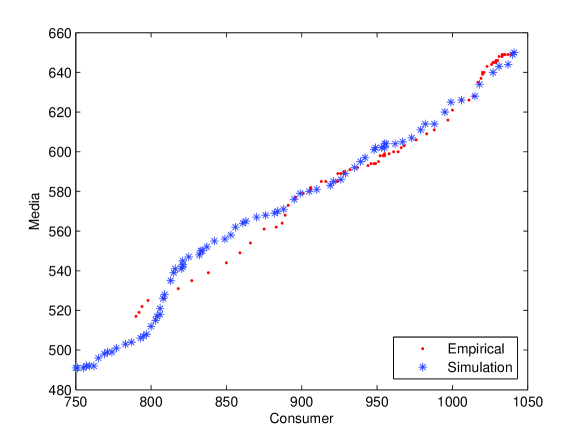
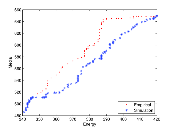
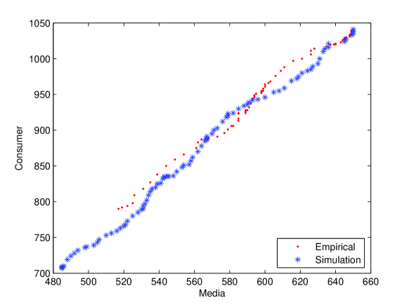
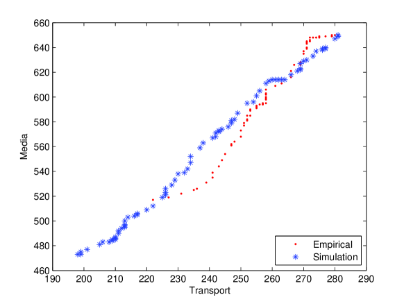
Figure 2: Number of Surviving Bonds in Matched Sectors.

To apply the two measures CRVaR and CRES in the proposed model, we consider some hypothetical values for the loss. The loss $L(W_{T},T)$, for each $T=1,2,\ldots,X_{0}$ and $W_{T}=0,1,\ldots,X_{0}$, are as in (30). Then we present the value of CRVaR and CRES for the proposed model as well as the two-sector model Ching et al. (2010) in Table 6. And the loss distribution are presented in figure 3.

$$\left\{\begin{array}[]{l}L(0,j)=j-1+0.1,\ {\rm for\ each}\ j=1,2,\ldots,X_{0};\\ L(i,j)=L(0,j)+i-1,\ {\rm for\ each}\ i=1,2,\ldots,X_{0}\ {\rm and}\ j=1,\dots,X_{0}.\\ \end{array}\right.$$ (30)

Sector A	Consumer	Energy	Media	Transport
Sector B	Media	Media	Consumer	Media
Proposed Model
CRVaR$(\beta=0.05)$	374.1	25.1	122.1	26.1
CRES$(\beta=0.05)$	424.7	33.8	150.4	33.8
CRVaR$(\beta=0.01)$	457.1	39.1	168.1	39.1
CRES$(\beta=0.01)$	495.1	47.5	192.4	46.5
Two-sector Model Ching et al. (2010)
CRVaR$(\beta=0.05)$	114.1	12.1	34.1	10.10
CRES$(\beta=0.05)$	146.1	17.1	45.7	14.1
CRVaR$(\beta=0.01)$	166.1	20.1	52.1	16.1
CRES$(\beta=0.01)$	195.6	24.5	63.3	20.2

Table 6: CRVaR and CRES

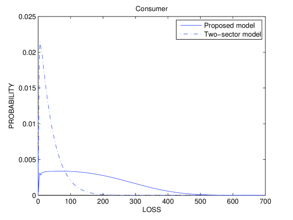
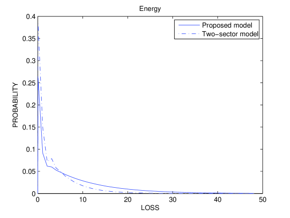
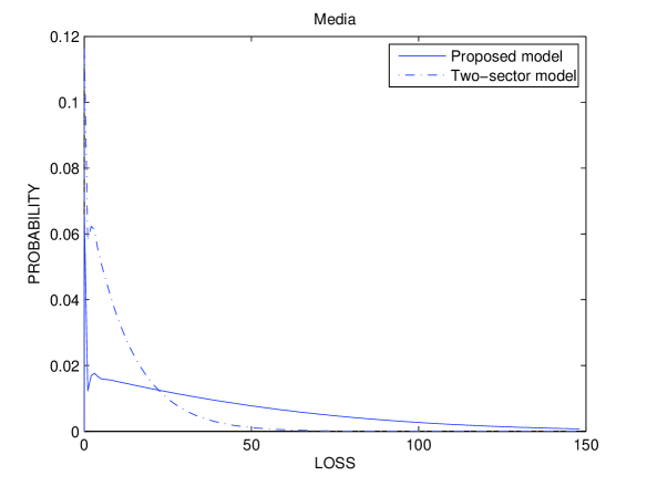
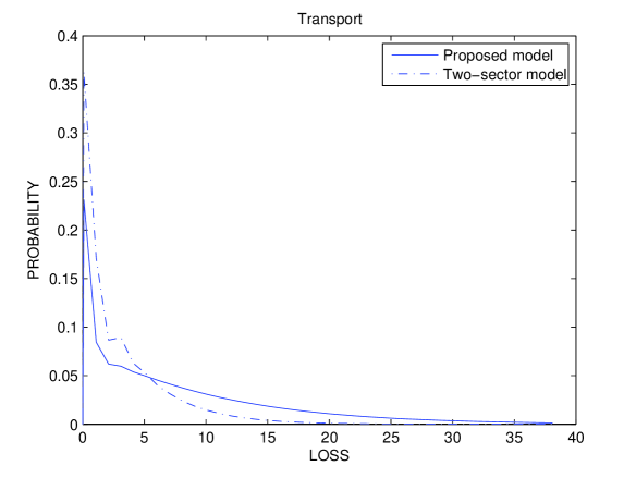
Figure 3: Loss distribution for proposed model and two-sector model Ching et al. (2010).

From Table 6, we see that for all of the four sectors, the existing two-sector model underestimates both the CRES and CRVaR. This reflects that failure to incorporate the contagion effect described in our proposed model leads to an underestimation of credit risk and has important consequences for credit risk management, such as inadequate capital charges for credit portfolios. Indeed, the loss distribution implied by the proposed model has a much fatter tail than that arising from the existing two-sector model. This explains why the proposed model provides more prudent estimates for the risk measures than the existing two sector model via incorporating contagion. We also remark that the contagion model including the causality of defaults in both direction, (i.e., looping defaults), has a significant impact on the loss distribution.

5 A Generalized Model

As in the basic model, the stochastic process $(X_{t},Y_{t})$ has the Markov property, where conditioning on $(X_{t},Y_{t})$, $(X^{1}_{t+1},Y^{1}_{t+1})$ and $(X^{2}_{t+1},Y^{2}_{t+1})$ are stochastically independent. The joint probability distribution, given the realization of $(X_{t},Y_{t}),\alpha_{t},\beta_{t}$, is given by:

$$\begin{array}[]{lll}p_{(x_{t},y_{t}),(\alpha_{t},\beta_{t})}(x_{t+1},y_{t+1})&=&P\{(X_{t+1},Y_{t+1})=(x_{t+1},y_{t+1})\mid(X_{t},Y_{t})=(x_{t},y_{t}),\alpha_{t},\beta_{t}\}\\ &=&\left(\begin{array}[]{c}x^{1}_{t}\\ y^{1}_{t+1}\end{array}\right){(\alpha}_{t})^{y^{1}_{t+1}}(1-{\alpha}_{t})^{x^{1}_{t+1}}\times\left(\begin{array}[]{c}x^{2}_{t}\\ y^{2}_{t+1}\end{array}\right){(\beta}_{t})^{y^{2}_{t+1}}(1-{\beta}_{t})^{x^{2}_{t+1}}.\\ \end{array}$$ (37)

However, instead of maintaining the specific form of a bivariate step function for $\alpha_{t},\beta_{t}$, this model assumes that $\alpha_{t}$ and $\beta_{t}$ follow certain Beta distributions depending on $(X_{t},Y_{t})$. By assuming a beta density on the unknown transition parameters, the chain becomes a Markov chain with transition matrix containing random parameters. This allow us to incorporate parameter uncertainty while, at the same time, retaining the analytical tractability of the model. For each time period, the number of defaults has the Beta-binomial distribution depending on the number of defaults in last time period. The Beta-binomial distribution is extensively used in Bayesian statistics, empirical Bayes methods and classical statistics as an overdispersed binomial distribution.

Specifically, it is assumed that the density of $\alpha_{t}$ and $\beta_{t}$ are given by $f_{\alpha}(x;(X_{t},Y_{t}))$ and $f_{\beta}(x;(X_{t},Y_{t}))$, respectively, and

$$f_{\alpha}(x;(X_{t},Y_{t}))=\sum_{i=0}^{3}\frac{h_{i}(y^{1}_{t},y^{2}_{t})}{B(A_{i1},A_{i2})}x^{A_{i1}-1}(1-x)^{A_{i2}-1}$$

and

$$f_{\beta}(x;(X_{t},Y_{t}))=\sum_{i=0}^{3}\frac{h_{i}(y^{2}_{t},y^{1}_{t})}{B(B_{i1},B_{i2})}x^{B_{i1}-1}(1-x)^{B_{i2}-1}$$

where

$$B(x,y)=\int_{0}^{1}t^{x-1}(1-t)^{y-1}dt$$

and $A_{ij},B_{ij},i=0,1,2,3,j=1,2$ are parameters of the Beta distribution. From the definition, one can have the following transition probability:

$$\begin{array}[]{ll}&P\{(X^{1}_{t+1},Y^{1}_{t+1})=(x^{1}_{t+1},y^{1}_{t+1})\mid(X_{t},Y_{t})=(x_{t},y_{t})\}\\ =&\left(\begin{array}[]{c}x^{1}_{t}\\ y^{1}_{t+1}\end{array}\right){E\left[({\alpha}_{t})^{y^{1}_{t+1}}(1-{\alpha}_{t})^{x^{1}_{t+1}}\mid(X_{t},Y_{t})=(x_{t},y_{t})\right]}\\ =&\left(\begin{array}[]{c}x^{1}_{t}\\ y^{1}_{t+1}\end{array}\right)\displaystyle\int_{0}^{1}p^{y^{1}_{t+1}}(1-p)^{x^{1}_{t+1}}f_{\alpha}(p;(x_{t},y_{t}))dp\\ =&\left(\begin{array}[]{c}x^{1}_{t}\\ y^{1}_{t+1}\end{array}\right){\displaystyle\sum_{i=0}^{3}}\displaystyle\frac{h_{i}(y^{1}_{t},y^{2}_{t})}{B(A_{i1},A_{i2})}\int_{0}^{1}p^{y^{1}_{t+1}}(1-p)^{x^{1}_{t+1}}p^{A_{i1}-1}(1-p)^{A_{i2}-1}dp\\ =&\left(\begin{array}[]{c}x^{1}_{t}\\ y^{1}_{t+1}\end{array}\right){\displaystyle\sum_{i=0}^{3}}h_{i}(y^{1}_{t},y^{2}_{t})\displaystyle\frac{B(y^{1}_{t+1}+A_{i1},x^{1}_{t+1}+A_{i2})}{B(A_{i1},A_{i2})}\end{array}$$ (38)

A similar transition probability distribution is shared with the number of defaults in Sector B.

$$\begin{array}[]{ll}&P\{(X^{2}_{t+1},Y^{2}_{t+1})=(x^{2}_{t+1},y^{2}_{t+1})\mid(X_{t},Y_{t})=(x_{t},y_{t})\}\\ =&\left(\begin{array}[]{c}x^{2}_{t}\\ y^{2}_{t+1}\end{array}\right){\displaystyle\sum_{i=0}^{3}}h_{i}(y^{2}_{t},y^{1}_{t})\displaystyle\frac{B(y^{2}_{t+1}+B_{i1},x^{2}_{t+1}+B_{i2})}{B(B_{i1},B_{i2})}\end{array}$$ (39)

From the transition probability distribution, to obtain a closed-form solution for a maximum likelihood estimate is difficult, if not impossible. However, we can compute the maximum likelihood estimates using numerical optimization.

5.1 Default Cycle and Severity

To derive the joint distribution of $(W^{i}_{T_{i}},T_{i})$ for $i=1,2$, we repeat the same steps in Section 2 to compute

$$P_{n}(x_{1},x_{2},h)=P\{T_{1}\geq n+1,X^{1}_{n}=x_{1},X^{2}_{n}=x_{2},I_{\{Y^{2}_{n}>0\}}=h\}.$$

Lemma 2

$$\begin{array}[]{ll}P_{n}(x_{1},x_{2},0)=&{\displaystyle\sum_{s_{1}>x_{1}}{s_{1}\choose x_{1}}}\left[\displaystyle P_{n-1}(s_{1},x_{2},0)\frac{B(s_{1}-x_{1}+A_{11},x_{1}+A_{12})}{B(A_{11},A_{12})}\frac{B(B_{21},x_{2}+B_{22})}{B(B_{21},B_{22})}\right.\\ &\displaystyle\left.+P_{n-1}{(s_{1},x_{2},1)}\frac{B(s_{1}-x_{1}+A_{31},x_{1}+A_{32})}{B(A_{31},A_{32})}\frac{B(B_{31},x_{2}+B_{32})}{B(B_{31},B_{32})}\right]\end{array}$$ (40)

$$\begin{array}[]{ll}P_{n}(x_{1},x_{2},1)=&{\displaystyle\sum_{s_{1}>x_{1}}\sum_{s_{1}>x_{1}}{s_{1}\choose x_{1}}{s_{2}\choose x_{2}}}\left[P_{n-1}(s_{1},s_{2},0)\frac{B(s_{1}-x_{1}+A_{11},x_{1}+A_{12})}{B(A_{11},A_{12})}\frac{B(s_{2}-x_{2}+B_{21},x_{2}+B_{22})}{B(B_{21},B_{22})}\right.\\ &\displaystyle\left.+P_{n-1}(s_{1},s_{2},1)\frac{B(s_{1}-x_{1}+A_{31},x_{1}+A_{32})}{B(A_{31},A_{32})}\frac{B(s_{2}-x_{2}+B_{31},x_{2}+B_{32})}{B(B_{31},B_{32})}\right]\end{array}$$ (41)

where the initial condition is given by

$$P_{0}(x_{1},x_{2},h)=\left\{\begin{array}[]{ll}1,&(x_{1},x_{2},h)=(x^{1}_{0},x^{2}_{0},1)\\ 0,&otherwise\end{array}\right.$$

Proof: We prove the first equality. The proof of the second one is similar. As in the proof of Lemma 1,

$$\begin{array}[]{lll}&P_{n}(x_{1},x_{2},0)\\ =&{\displaystyle\sum_{s_{1}>x_{1}}\sum_{h=0,1}}P_{n-1}(s_{1},x_{2},h)\\ &\times P\{Y^{1}_{n}>0,X^{1}_{n}=x_{1},X^{2}_{n}=x_{2},I_{\{Y^{2}_{n}>0\}}=0\mid Y^{1}_{n-1}>0,X^{1}_{n-1}=s_{1},X^{2}_{n-1}=x_{2},I_{\{Y^{2}_{n-1}>0\}}=h\}\end{array}$$

Note that by (38) and (39),

$$\begin{array}[]{ll}&P\{Y^{1}_{n}>0,X^{1}_{n}=x_{1},X^{2}_{n}=x_{2},I_{\{Y^{2}_{n}>0\}}=0\mid Y^{1}_{n-1}>0,X^{1}_{n-1}=s_{1},X^{2}_{n-1}=x_{2},I_{\{Y^{2}_{n-1}>0\}}=0\}\\ =&\displaystyle{s_{1}\choose x_{1}}\frac{B(s_{1}-x_{1}+A_{11},x_{1}+A_{12})}{B(A_{11},A_{12})}\frac{B(B_{21},x_{2}+B_{22})}{B(B_{21},B_{22})}\end{array}$$

and

$$\begin{array}[]{ll}&P\{Y^{1}_{n}>0,X^{1}_{n}=x_{1},X^{2}_{n}=x_{2},I_{\{Y^{2}_{n}>0\}}=0\mid Y^{1}_{n-1}>0,X^{1}_{n-1}=s_{1},X^{2}_{n-1}=x_{2},I_{\{Y^{2}_{n-1}>0\}}=1\}\\ =&\displaystyle{s_{1}\choose x_{1}}\frac{B(s_{1}-x_{1}+A_{31},x_{1}+A_{32})}{B(A_{31},A_{32})}\frac{B(B_{31},x_{2}+B_{32})}{B(B_{31},B_{32})}\end{array}$$

Combining these two results, (40) follows.

Hence the joint distribution of $(T_{1},W^{1}_{T_{1}})$ follows

Proposition 3

$$\begin{array}[]{ll}P\{(T_{1},W^{1}_{T_{1}})=(n,x))\}=&\displaystyle\sum_{x_{2}}P_{n-1}(x^{1}_{0}-x,x_{2},0)\frac{B(A_{11},x^{1}_{0}-x+A_{12})}{B(A_{11},A_{12})}\\ &\displaystyle+\sum_{x_{2}}P_{n-1}(x^{1}_{0}-x,x_{2},1)\frac{B(A_{31},x^{1}_{0}-x+A_{32})}{B(A_{31},A_{32})}\end{array}$$ (42)

Proof: As in the proof of Proposition 1,

$$\begin{array}[]{lll}&P\{(T_{1},W^{1}_{T_{1}})=(n,x)\}\\ =&{\displaystyle\sum_{x_{2}}\sum_{h=0,1}}P_{n-1}(x^{1}_{0}-x,x_{2},h)\\ &\times P\{Y^{1}_{n}=0,X^{1}_{n}=x^{1}_{0}-x\mid Y^{1}_{n-1}>0,X^{1}_{n-1}=x^{1}_{0}-x,X^{2}_{n-1}=x_{2},I_{\{Y^{2}_{n-1}>0\}}=h\}\end{array}$$

Note that by (38),

$$\begin{array}[]{ll}&P\{Y^{1}_{n}=0,X^{1}_{n}=x^{1}_{0}-x\mid Y^{1}_{n-1}>0,X^{1}_{n-1}=x^{1}_{0}-x,X^{2}_{n-1}=x_{2},I_{\{Y^{2}_{n-1}>0\}}=0\}\\ =&\displaystyle\frac{B(A_{11},x^{1}_{0}-x+A_{12})}{B(A_{11},A_{12})}\end{array}$$

and

$$\begin{array}[]{ll}&P\{Y^{1}_{n}=0,X^{1}_{n}=x^{1}_{0}-x\mid Y^{1}_{n-1}>0,X^{1}_{n-1}=x^{1}_{0}-x,X^{2}_{n-1}=x_{2},I_{\{Y^{2}_{n-1}>0\}}=1\}\\ =&\displaystyle\frac{B(A_{31},x^{1}_{0}-x+A_{32})}{B(A_{31},A_{32})}\end{array}$$

Combining these two, (42) follows.

6 Concluding Remarks

We propose a two-sector Markovian infectious model. The proposed model incorporated two important features of credit contagion, namely, the chain reactions of defaults and the bi-lateral causality of defaults between two industrial sectors. We capture the chain reactions of defaults by postulating that the future default probability switches over time according to the current number of defaults of two industrial sectors. The bi-lateral causality of defaults meant that defaults in one sector are caused by defaults in another sector, and vice versa. This bi-lateral causality of defaults enriches the dependent structures of credit risk model. We provide an efficient estimation method of the proposed model based on the maximum likelihood estimation. Two important risk measures, namely, the CRVaR and the CRES, were evaluated under the proposed model. To provide a more flexible and realistic modeling framework for the dynamics of default probabilities, we extend the model to a case where default probabilities are Beta random variables given the realization of the state in the previous time period.

We also conduct empirical studies on the credit risk models using real default data. We adopted the BIC to compare the proposed model with the existing two-sector model proposed in Ching et al. (2010). The numerical results reveal that the proposed two-sector model outperforms empirically the existing model. By comparing the risk measures evaluated from the proposed model and those evaluated from the existing two-sector model, we found that failure to incorporate the contagion effect described in the proposed model leads to an underestimation of risk measures. This provides some evidence to support the proposed model.

One possible topic for future research may be to incorporate the impact of the number of defaults on the likelihood of future defaults via a different parametrization of the future default probability. In current paper, we assumed that the joint future default probability switches over time depending on the region where the current number of defaults falls in. Four parameters, namely, $a_{0}$, $a_{1}$, $a_{2}$ and $a_{3}$ were involved. To provide a more parsimonious way to incorporate the current number of defaults on the joint future default probability, one may consider the following parametrization for the future default probability:

$$\alpha_{t}=a_{0}+a_{1}y^{1}_{t}+a_{2}y^{2}_{t}\ ,$$

where $y^{1}_{t}$ and $y^{2}_{t}$ are the current numbers of defaults in the two industrial sectors. Using this parametrization, we can reduce the number of parameters by one and accounts for more information of the current number of defaults when evaluating the future default probability.

Acknowledgment: The authors would like to thank the anonymous referees for their helpful comments. Research supported in part by RGC Grants 7017/07P, HKU CRCG Grants and HKU Strategic Research Theme Fund on Computational Physics and Numerical Methods.

References

- [1] Black, F. and Scholes, M. (1973). “The Pricing of Options and Corporate Liabilities,” Journal of Political Economy, 81(3), p. 637-654
- [2] Ching, W., Leung, H., Jiang, H., Sun, L. and Siu, T. (2010). “A Markovian Network Model for Default Risk Management,” International Journal of Intelligent Engineering Informatics, 1(1), p. 104-124.
- [3] Ching, W., Siu, T., Li, L., Li, T. and Li, W. (2008). “On an Infectious Model for Default Crisis,” http://www.hku.hk/math/imr/IMRPrePrintSeries/2007/IMR2007-21.pdf
- [4] Daley, D. and Gani, J. (1999). Epidemic modeling: an introduction. Cambridge University Press.
- [5] Davis, M., Lo, V. (2001). “Infectious Defaults,” Quantitative Finance, 1(4), p. 382-387.
- [6] Giampieri, G., Davis, M. and Crowder, M. (2005). “Analysis of Default Data Using Hidden Markov Models,” Quantitative Finance, 5(1), p. 27-34.
- [7] Gu, J., Ching, W. and Siu, T. (2011). “A Markovian Infectious Model for Dependent Default Risk,” International Journal of Intelligent Engineering Informatics, 1(2), p. 174-195
- [8] Jarrow, R., and Turnbull, S. (1995). “Pricing derivatives on financial securities subject to credit risk,” Journal of Finance, 50(1), p. 53-85.
- [9] Jarrow, R., Yu, F. (2001). “Counterparty risk and the pricing of defaultable securities,” Journal of Finance, 56, p.1765-1799.
- [10] Li, D. (2000). “On default correlation: a Copula function approach,” Journal of Fixed Income, 9(4), p. 43-54.
- [11] Merton, R.(1974). “On the Pricing of Corporation Debt: The Risk Structure of Interest Rates,” Journal of Finance, 29(2), p. 449-470.