Semi-implicit scheme for treating radiation under M1 closure in general relativistic conservative fluid dynamics codes

Abstract

A numerical scheme is described for including radiation in multi-dimensional general-relativistic conservative fluid dynamics codes. In this method, a covariant form of the M1 closure scheme is used to close the radiation moments, and the radiative source terms are treated semi-implicitly in order to handle both optically thin and optically thick regimes. The scheme has been implemented in a conservative general relativistic radiation hydrodynamics code KORAL. The robustness of the code is demonstrated on a number of test problems, including radiative relativistic shock tubes, static radiation pressure supported atmosphere, shadows, beams of light in curved spacetime, and radiative Bondi accretion. The advantages of M1 closure relative to other approaches such as Eddington closure and flux-limited diffusion are discussed, and its limitations are also highlighted.

1 Introduction

Accretion disks are the power source behind many astrophysical systems. They span a wide range of central object mass, size and type, e.g., young stellar objects, neutron star binaries, black hole binaries, gamma-ray bursts, active galactic nuclei, to name a few, and exhibit a variety of different regimes of physics. In many systems, radiation is so intense that it strongly couples to the accreting gas and dramatically alters the flow structure and dynamics. To correctly infer the physics of such systems, we need models that properly take into account the interaction of gas and radiation.

Proper treatment of radiation is especially important for black holes (BHs) near the Eddington luminosity limit, $L_{\rm Edd}$. Transient black hole binaries (BHBs) approach near-Eddington accretion rates near the peak of their outbursts (McClintock & Remillard, 2006; Remillard & McClintock, 2006; Done, Gierliński & Kubota, 2007), while some exceptional BHBs spend extended periods of time with $L\gtrsim L_{\rm Edd}$ (e.g., SS433, Margon et al. 1979; Margon 1984; GRS1915+105, Fender & Belloni 2004). Ultra-luminous X-ray sources have even larger luminosities and may conceivably be highly super-Eddington stellar-mass BHs (Watarai et al., 2001), or intermediate mass BHs accreting at close to Eddington (Miller & Colbert, 2004). In either case, radiation must play an important role. Finally, luminous active galactic nuclei, especially those whose supermassive BHs (SMBHs) are growing rapidly in mass, may be perfect examples of systems with closely coupled gas and radiation (Collin et al., 2002).

Since most of the radiation from an accretion disk originates in the inner regions, general relativistic (GR) effects play an important role in determining the emergent radiation spectrum. Treating the interaction of fluid dynamics and radiation quantitatively in GR numerical codes is a daunting task that has been achieved only recently and only for optically thick flows, as we discuss below. However, the emergent spectrum is established at an optical depth of order unity, $\tau\sim 1$, which requires a proper treatment of the optically-thick disk ($\tau\gg 1$), the optically-thin corona ($\tau\ll 1$) if one is present, and the optically thick-to-thin transition in between. In this paper, we present a GR numerical radiation hydrodynamics technique and a code which handles all three regimes of optical depth.

Depending on the mass accretion rate, a given accretion system can switch between different spectral states, with different radiation mechanisms dominating and with varying degrees of coupling between radiation and gas. At very low accretion rates, $L/L_{\rm Edd}\ll 10^{-2}$, e.g., Sgr A^∗ the SMBH at our Galactic Center (Narayan, Yi, & Mahadevan, 1995), the accretion flow advects most of the viscously released energy into the BH rather than radiating the energy (some energy probably also flows out in a wind). Such flows are optically thin, radiatively inefficient and geometrically thick, and are called advection-dominated accretion flows (ADAFs, see Narayan & Yi 1994, 1995; Abramowicz et al. 1995). Analytical and semi-analytical models are reasonably successful in accounting for the main features in the spectra of ADAFs (e.g., Yuan, Quataert, & Narayan 2003). However, it was realized early on that numerical simulations are necessary to understand properly the physics of ADAFs.

The low optical depth and the extreme radiative inefficiency of an ADAF are a major advantage for simulations since they allow one to solve the fluid dynamics separately from the radiation field A number of sophisticated GR magnetohydrodynamic (GRMHD) codes have been developed (e.g., De Villiers et al., 2003; Gammie et al., 2003; Anninos et al., 2005; Del Zanna et al., 2007), and ADAF-like models have been simulated using these (see Narayan et al. 2012; McKinney et al. 2012; Tchekhovskoy & McKinney 2012 for recent work). To compute observables, the output from such pure GRMHD codes are usually post-processed with stand-alone radiation transfer schemes (e.g. Schnittman et al., 2006; Shcherbakov et al., 2010). Alternatively, a simple local cooling prescription is included directly into the code (e.g., Fragile & Meier, 2009; Dibi et al., 2012); this is not difficult since the gas is optically thin, so no radiative transfer is involved.

For higher accretion rates, $10^{-2}\lesssim L/L_{\rm Edd}\lesssim 0.3$, efficient cooling sets in, and the inner accretion disk collapses into an optically thick geometrically thin accretion disk (Narayan & Yi, 1995; Esin et al., 1997, 1998; Meyer-Hofmeister & Meyer, 2003; McClintock & Remillard, 2006; Done, Gierliński & Kubota, 2007). This state of accretion is the best understood of all states, and its thermal black-body-like spectrum is well-described by the standard thin disk model with $\alpha$ viscosity (Shakura & Sunyaev, 1973; Novikov & Thorne, 1973; Frank et al., 2002). However, despite its many successes, the $\alpha$ disk model cannot describe important microphysical aspects of the flow, e.g., thermal and viscous stability, vertical structure of the disk, and the role of magnetic fields. Moreover, optically thick, geometrically thin disks are much more difficult to simulate numerically because of the strong coupling between gas and radiation.

Only a few time-dependent GRMHD numerical simulations of thin disks have been computed so far, and all are based on an ad hoc (although physically motivated) local cooling function which artificially removes excess heat to keep the disk geometrically thin (Shafee et al. 2008; Penna et al. 2010; Noble et al. 2011; see also Reynolds & Fabian 2008). Although this approach has produced valuable results on the dynamics of the gas, it misses real physics involving propagation of photons along curved geodesics, radiation pressure support, radiative winds, etc.

Using a flux-limited diffusion approximation, small patches of radiatively efficient thin accretion disks have been simulated using the local shearing box approximation (Turner et al., 2003; Krolik et al., 2007; Blaes et al., 2007, 2011; Hirose et al., 2009a, b), and even a few full disk simulations have been done with a non-relativistic code using flux-limited diffusion (Ohsuga et al., 2009; Ohsuga & Mineshige, 2011). However, to model a radiatively efficient disk self-consistently it is necessary to handle the radiation field in both the optically thick (disk interior) and optically thin (corona) limits. This is difficult with the flux-limited diffusion approximation which artificially enforces the flux to follow the local gradient of the radiative energy density. Fueled by advances in radiation algorithms, more advanced radiation moment closures are now becoming possible, which allow accurate treatment of both optically thick and thin photon fields in the “instant light” (nonrelativistic) approximation (Hayes & Norman, 2003; González et al., 2007; Jiang et al., 2012; Davis et al., 2012). However, as we discuss below, GR radiation transfer codes still continue to rely on flux-limited diffusion or the Eddington approximation.

At super-Eddington accretion rates, $L/L_{\rm Edd}\gtrsim 1$, accretion flows again become radiatively inefficient. Here, the optical depth is so large that the photon diffusion time from the disk interior to the photosphere becomes longer than the accretion time. As a result, most of the photons are advected with the gas into the BH, leading to a “slim accretion disk” (Abramowicz et al., 1988). This important but poorly understood accretion state may be responsible for much of the SMBH mass growth in the Universe; for instance, it might explain the paradox of having $10^{9}M_{\odot}$ BHs already at $z>6$, when the Universe was less than $1$ Gyr old (Barth et al., 2003; Willott et al., 2005; Fan et al., 2006; Willott et al., 2010; Mortlock et al., 2011). Super-Eddington accretion may also apply to ultra-luminous X-ray sources (e.g., Watarai et al., 2001; Kawashima et al., 2012). Clearly, to understand the accretion physics in these systems, radiation MHD models that self-consistently couple gas, radiation and magnetic fields, are crucial. Such models are also important for measuring BH spins (McClintock et al., 2011; Straub et al., 2011), calculating the radiative efficiency of super-Eddington accretion disks (e.g., Sa̧dowski, 2009), and understanding large-scale cosmological feedback by radiation-driven outflows from AGN (see Fabian 2012 for an observational review). Some efforts have already been made on attacking these important problems. In particular, using a non-relativistic code and flux-limited diffusion, super-Eddington accretion flows have been simulated and their spectra computed (Ohsuga et al., 2003; Ohsuga, 2006; Ohsuga & Mineshige, 2011; Kawashima et al., 2012).

Until a few years ago, all radiation hydrodynamic and MHD simulations of accretion disks were run with non-relativistic or special relativistic codes. However, physics around BHs must be studied in GR because of the the strong gravity involved. Recently, progress has been made in implementing radiation into GR codes. Farris et al. (2008) developed a formalism for incorporating radiation under the Eddington approximation in a conservative MHD code. This method has been implemented in other codes (Zanotti et al., 2011; Fragile et al., 2012), but all these codes have problems because of the stiffness of radiative source terms at large optical depths. These stiff terms require implicit treatment, which is prohibitively complicated in curved space-time. Roedig et al. (2012), extended the method by applying an implicit-explicit Runge-Kutta numerical scheme. However, the authors again relied on the Eddington approximation, which cannot handle optically thin flows accurately. A more advanced method has been recently described by Shibata & Sekiguchi (2012), who employ a truncated moment formalism, similar to our method, for neutrino transport in GR.

In the present paper, we describe a simple approach for including radiation transport in GR codes. The method makes use of a key simplification that is intrinsic to GR applications. Normally, in non-relativistic codes, hydrodynamic or MHD signal speeds, which determine the time step via the Courant condition, are much slower than the speed of light. Correspondingly, the time step that one uses to evolve the fluid equations is much longer than the light-crossing time across a cell. This is a problem when one wants to simulate radiation hydrodynamical systems, especially in optically thin regions, where one is faced with a large mis-match between the characteristic speeds of the fluid and the radiation. Either one must limit the time step to the light-crossing time, which prohibitively increases the computational cost (as the fluid dynamics evolve on a much slower time scale), or one must handle all the radiation terms via an implicit method. The latter inevitably couples neighboring cells and makes the code very complicated. Moreover, it does not easily generalize to curved space-time.

In contrast, a GR code is applied only in relativistic space-times near BHs and neutron stars. The time step in simulations is generally set by applying the Courant condition to the smallest grid cell, located at the innermost radius, where the flow is relativistic. Thus, the normal time step in a pure GR hydro or GRMHD code is already limited by the speed of light. Therefore, including radiation as an extra relativistic fluid is fairly easy. In particular, the advection terms in the radiation equations are no more difficult to compute than the corresponding terms in the fluid and magnetic field evolution equations. Nor does the time step need to be adjusted in any way. Because of this large simplification, the advective radiation operator can be treated via a standard explicit approach, just as one handles the corresponding hydro and MHD terms.

Of course, the interactions between radiation and gas via emission, absorption and scattering introduce their own time scales. These can sometimes be very short, requiring implicit handling. However, these interactions are local and can be handled via a local implicit scheme. This is a great simplification. It means that one can do implicit evolution independently in each grid cell, without coupling to other cells. Therefore, there are no space-time curvature effects to contend with as in other more sophisticated multi-cell implicit schemes in GR.

In the work described here, we have implemented the above approach, closing the radiation moment equations using the M1 closure scheme (Levermore, 1984; Dubroca & Feugeas, 1999; González et al., 2007). M1 closure allows a limited treatment of anisotropic radiation fields and works well in both optically thick and thin regimes. We have implemented our method in a GR radiation hydrodynamics (GRRHD) code KORAL. The structure of the paper is as follows: In Section 2 we introduce the equations, in Section 3 we describe the numerical algorithm used by KORAL, in Section 4 we present a set of test problems which validate the scheme, and in Section 5 we discuss possible applications of the code.

2 Equations

2.1 Conservation laws

A pure hydrodynamic flow is described by the following conservation laws,

$$\hskip 72.26999pt(\rho u^{\mu})_{;\mu} = 0,$$ (1)

$$\hskip 72.26999pt(T^{\mu}_{\nu})_{;\mu} = 0,$$ (2)

where $\rho$ is the gas density in the comoving fluid frame, $u^{\mu}$ is the gas four-velocity as measured in the “lab frame”, and $T^{\mu}_{\nu}$ is the hydrodynamical stress-energy tensor in this frame,

$$T^{\mu}_{\nu}=(\rho+u+p)u^{\mu}u_{\nu}+p\delta^{\mu}_{\nu},$$ (3)

with $u$ and $p$ representing the internal energy and pressure of the gas in the comoving frame.

In the case of radiation hydrodynamics, it is convenient to introduce the radiation stress-energy tensor $R^{\mu}_{\nu}$ (e.g., Mihalas & Mihalas, 1984), and to replace the second equation above with the more general conservation law,

$$(T^{\mu}_{\nu}+R^{\mu}_{\nu})_{;\mu}=0.$$ (4)

The radiation stress-energy tensor in an orthonormal frame comprises various moments of the specific intensity $I_{\nu}$, e.g., in the fluid frame it takes the following form,

$$\widehat{R}=\left[\begin{array}[]{cc}\widehat{E}&\widehat{F}^{i}\\ \widehat{F}^{j}&\widehat{P}^{ij}\end{array}\right],$$ (5)

where the fluid-frame quantities

$$\hskip 72.26999pt\widehat{E} = \int\widehat{I}_{\nu}{\,\rm d\nu\,d\Omega},$$ (6)

$$\hskip 72.26999pt\widehat{F}^{i} = \int\widehat{I}_{\nu}{\,\rm d\nu\,d\Omega\,N^{i}},$$ (7)

$$\hskip 72.26999pt\widehat{P}^{ij} = \int\widehat{I}_{\nu}{\,\rm d\nu\,d\Omega\,N^{i}\,N^{j}}$$ (8)

are the radiation energy density, the radiation flux and the radiation pressure tensor, respectively, and $N^{i}$ is a unit vector in direction $x^{i}$.

The fluid frame radiation stress tensor $\widehat{R}$ is related to the tensor $\tilde{R}$ defined in the locally flat non-rotating frame, or the zero-angular momentum frame (ZAMO) (Bardeen et al., 1972), by

$$\tilde{R}^{\mu\nu}=\Lambda^{\mu}_{\alpha}(\tilde{u})\Lambda^{\nu}_{\beta}(\tilde{u})\widehat{R}^{\alpha\beta},$$ (9)

where $\Lambda$ is the Lorentz boost,

$$\Lambda(\tilde{u})=\left[\begin{array}[]{cc}\gamma&\gamma\tilde{v}^{i}\\ \gamma\tilde{v}^{j}&\delta^{ij}+\frac{\tilde{v}^{i}\tilde{v}^{j}(\gamma-1)}{\tilde{v}^{2}}\\ \end{array}\right],$$ (10)

$\gamma=\tilde{u}^{t}$, $\tilde{v}^{i}=\tilde{u}^{i}/\tilde{u}^{t}$, and $\tilde{u}^{\mu}$ is the four-velocity of the gas as measured by the locally non-rotating observer.

Quantities in the ZAMO frame (denoted with tildes) are related to those in the lab frame by tensors created from the components of the corresponding tetrads of the ZAMO, $e^{\mu}_{\nu}$ and $\tilde{e}^{\mu}_{\nu}$, defined in Bardeen et al. (1972). The radiation tensor transforms as

$$\hskip 72.26999ptR^{\mu\nu} = e^{\mu}_{\alpha}e^{\nu}_{\beta}\tilde{R}^{\alpha\beta},$$ (11)

$$\hskip 72.26999pt\tilde{R}^{\mu\nu} = \tilde{e}^{\mu}_{\alpha}\tilde{e}^{\nu}_{\beta}R^{\alpha\beta},$$ (12)

while four-vectors transform as

$$\hskip 72.26999ptu^{\mu} = e^{\mu}_{\alpha}\tilde{u}^{\alpha},$$ (13)

$$\hskip 72.26999pt\tilde{u}^{\mu} = \tilde{e}^{\mu}_{\alpha}u^{\alpha}.$$ (14)

The conservation law (4) may be rewritten with the help of the radiation four-force density $G^{\nu}$ as

$$\hskip 72.26999pt(T^{\mu}_{\nu})_{;\mu} = G_{\nu},$$ (15)

$$\hskip 72.26999pt(R^{\mu}_{\nu})_{;\mu} = -G_{\nu},$$

where $G^{\nu}$ is given by (Mihalas & Mihalas, 1984),

$$G^{\nu}=\int(\chi_{\nu}I_{\nu}-\eta_{\nu}){\,\rm d\nu\,d\Omega\,N^{i}},$$ (16)

which takes a particularly simple form in the fluid frame,

$$\widehat{G}=\left[\begin{array}[]{c}\kappa(\widehat{E}-4\pi\widehat{B})\\ \chi\widehat{F}^{i}\end{array}\right].$$ (17)

Here, $\widehat{B}=\sigma T^{4}/\pi$ is the integrated Planck function corresponding to the gas temperature $T$, $\sigma$ is the Stefan-Boltzmann constant, $\chi_{\nu}$ and $\eta_{\nu}$ denote the frequency-dependent opacity and emissivity coefficients, respectively, while $\kappa$ and $\chi$ are the frequency integrated absorption and total opacity coefficients, respectively. In Section 4, we occasionally refer to the scattering opacity $\kappa_{\rm es}$, which is related to $\kappa$ and $\chi$ by

$$\chi\equiv\kappa+\kappa_{\rm es}.$$ (18)

The four-force $G^{\mu}$ may be transformed between frames as described above, e.g.,

$$G^{\mu}=e^{\mu}_{\alpha}\Lambda^{\alpha}_{\gamma}(\tilde{u})\widehat{G}^{\gamma}.$$ (19)

The rest mass conservation equation (1) and the energy-momentum conservation equations (15) may be written in a coordinate basis in the following conservative form (Gammie et al., 2003),

$$\hskip 21.68121pt\partial_{t}(\sqrt{-g}\rho u^{t})+\partial_{i}(\sqrt{-g}\rho u^{i}) = 0,$$ (20)

$$\hskip 21.68121pt\partial_{t}(\sqrt{-g}T^{t}_{\nu})+\partial_{i}(\sqrt{-g}T^{i}_{\nu}) = \sqrt{-g}T^{\kappa}_{\lambda}\Gamma^{\lambda}_{\nu\kappa}+\sqrt{-g}G_{\nu},$$ (21)

$$\hskip 21.68121pt\partial_{t}(\sqrt{-g}R^{t}_{\nu})+\partial_{i}(\sqrt{-g}R^{i}_{\nu}) = \sqrt{-g}R^{\kappa}_{\lambda}\Gamma^{\lambda}_{\nu\kappa}-\sqrt{-g}G_{\nu}.$$ (22)

This formulation has a drawback for numerical computations: the terms involving Christoffel symbols on the right, when calculated at cell centers, will not balance the corresponding spatial derivatives on the left (approximated under a given reconstruction scheme). This is true even for particularly simple situations such as constant gas or radiation pressure, and can lead to catastrophic secular errors. To solve this issue we can either modify the values of the Christoffel symbols suitably (Appendix A of McKinney et al. 2012) or we can reformulate the equations so as to avoid the problem. We choose the second approach and make use of the following equations,

$$\partial_{t}(\rho u^{t})+\partial_{i}(\rho u^{i})=-\frac{\rho u^{i}}{\sqrt{-g}}\partial_{i}(\sqrt{-g}),$$ (23)

$$\partial_{t}(T^{t}_{\nu})+\partial_{i}(T^{i}_{\nu})=T^{\kappa}_{\lambda}\Gamma^{\lambda}_{\nu\kappa}-\frac{T^{i}_{\nu}}{\sqrt{-g}}\partial_{i}(\sqrt{-g})+G_{\nu},$$ (24)

$$\partial_{t}(R^{t}_{\nu})+\partial_{i}(R^{i}_{\nu})=R^{\kappa}_{\lambda}\Gamma^{\lambda}_{\nu\kappa}-\frac{R^{i}_{\nu}}{\sqrt{-g}}\partial_{i}(\sqrt{-g})-G_{\nu},$$ (25)

where we assumed that the metric is static and moved its determinant out of the derivatives on the left. In this formulation, the two terms that are expected to cancel each other both appear as source terms and therefore are calculated at the same location.

2.2 Closure scheme

To close the above set of equations we need a prescription to compute the second moments of the angular radiation intensity distribution. Specifically, we need a prescription to write down the full radiation stress tensor $R^{\mu\nu}$ knowing only the radiative energy density $R^{tt}$ and the fluxes $R^{ti}$.

The simplest approach, which corresponds to assuming a nearly isotropic radiation field, is the Eddington approximation, which in the fluid frame gives

$$\widehat{P}^{ij}=\frac{1}{3}\widehat{E}\delta^{ij}.$$ (26)

However, the assumption of isotropic specific intensity is good only in optically thick media. In many astrophysical applications we are interested in radiation that escapes from the photosphere to infinity, for which we need a better closure scheme.

Following Levermore (1984), we assume that the radiation tensor is isotropic and satisfies the Eddington closure, not in the fluid frame, but in the orthonormal “rest frame” of the radiation. The latter is defined as the frame in which the radiative flux vanishes. Thus, in this frame, we assume that $\bar{R}^{tt}=\bar{E}$, $\bar{R}^{ii}=\bar{E}/3$, and all other components of $\bar{R}$ are zero. This leads to the M1 closure scheme.

In the radiation rest frame, the radiation stress tensor can be written in a compact form as

$$\bar{R}^{\mu\nu}=\frac{4}{3}\bar{E}\,\bar{u}^{\mu}_{R}\bar{u}^{\nu}_{R}+\frac{1}{3}\bar{E}\,g^{\mu\nu},$$ (27)

where $\bar{u}^{\mu}_{R}=\{1,0,0,0\}$ and $g^{\mu\nu}$ is the contravariant metric tensor, which in this frame is given by the flat space Minkowski metric. Since equation (27) is in a covariant form, it is also valid in the lab frame (as well as all other frames), with $u^{\mu}_{R}$ being the four-velocity of the radiation rest frame as measured by an observer in the lab frame. Note that, regardless of which frame one works in, the quantity $\bar{E}$ should be interpreted as the radiation energy density as measured in the radiation rest frame.

Each time step in the numerical integration in any particular cell gives an update to the “time” row of the radiation tensor, $R^{t\nu}$, for that cell in the lab frame. Thus, we obtain numerical values of these four particular components of the tensor. According to equation (27), the full tensor $R^{\mu\nu}$ is a function of 5 numbers, $\bar{E}$, $u^{\mu}_{R}$, though only four of these are independent since the norm of the four-velocity $u^{\mu}_{R}$ is equal to $-1$. Hence, we can use the four given tensor elements to solve for the four unknowns and thereby compute the full matrix. Below we give an algorithm for doing this analytically.

Consider the quantity $R^{t\mu}R^{t\nu}$ which can be expressed as (equation 27),

$$R^{t\mu}R^{t\nu}=\frac{1}{9}\bar{E}^{2}\left[16(u^{t}_{R})^{2}u^{\mu}_{R}u^{\nu}_{R}+4u^{t}_{R}u^{\mu}_{R}g^{t\nu}+4u^{t}_{R}u^{\nu}_{R}g^{t\mu}+g^{t\mu}g^{t\nu}\right].$$ (28)

If we contract this with $g_{\mu\nu}$ and use the following results,

$$\hskip 56.9055ptg_{\mu\nu}\,u^{\mu}_{R}u^{\nu}_{R} = -1,$$ (29)

$$\hskip 56.9055ptg_{\mu\nu}\,u^{\mu}_{R}g^{t\nu} = u_{\nu,R}\,g^{t\nu}=u^{t}_{R},$$ (30)

$$\hskip 56.9055ptg_{\mu\nu}\,g^{t\mu}g^{t\nu} = \delta^{t}_{\nu}\,g^{t\nu}=g^{tt},$$ (31)

we obtain

$$g_{\mu\nu}\,R^{t\mu}R^{t\nu}=-\frac{8}{9}\bar{E}^{2}(u^{t}_{R})^{2}+\frac{1}{9}\bar{E}^{2}g^{tt}.$$ (32)

The left-hand side is computable from the four given tensor elements and the right-hand side involves two of the unknowns: $\bar{E}$, $u^{t}_{R}$. We also have the following expression for $R^{tt}$,

$$R^{tt}=\frac{4}{3}\bar{E}(u^{t}_{R})^{2}+\frac{1}{3}\bar{E}g^{tt},$$ (33)

which again involves the same two unknowns. Thus, we can solve equations (32) and (33) to obtain $\bar{E}$ and $u^{t}_{R}$ (it reduces to a quadratic equation). It is then straightforward to calculate the remaining $u^{i}_{R}$ from the other time components of equation (27) and to calculate the entire radiation stress tensor.

For flat spacetime, the above formulation reduces to the standard formulae (Levermore, 1984; Dubroca & Feugeas, 1999; González et al., 2007). For instance, the radiation pressure tensor $\widehat{P}^{ij}$ in the fluid frame has the form,

$$\widehat{P}^{ij}=\left(\frac{1-\xi}{2}\delta^{ij}+\frac{3\xi-1}{2}\frac{f^{i}f^{j}}{|f|^{2}}\right)\widehat{E},$$ (34)

where $f^{i}=\widehat{F}^{i}/\widehat{E}$ is the reduced radiative flux and $\xi$ is the Eddington factor given by (Levermore, 1984),

$$\xi=\frac{3+4f^{i}f_{i}}{5+2\sqrt{4-3f^{i}f_{i}}}.$$ (35)

In the extreme “optically thick limit”, $\widehat{F}^{i}\approx 0$, and we find $f^{i}=0$, $f^{i}f_{i}=0$ and $\xi=1/3$, which corresponds to the correct answer, viz., the Eddington approximation,

$$\widehat{P}^{ij}_{\tau\gg 1}=\left[\begin{array}[]{ccc}1/3&0&0\\ 0&1/3&0\\ 0&0&1/3\\ \end{array}\right]\widehat{E}.$$ (36)

In the opposite extreme “optically thin limit”, $\widehat{F}^{1}=\widehat{E}$, i.e., a uni-directional radiation field directed along the x-axis, we have $f^{i}=\delta^{i}_{1}$, $f^{i}f_{i}=1$ and $\xi=1/3$, which gives

$$\widehat{P}^{ij}_{\tau\ll 1}=\left[\begin{array}[]{ccc}1&0&0\\ 0&0&0\\ 0&0&0\\ \end{array}\right]\widehat{E},$$ (37)

This corresponds to an intensity distribution in the form of a Dirac $\delta$-function parallel to the flux vector, which is again the correct answer. The M1 closure scheme thus handles both optical depth extremes well and it is found to be fairly good at intermediate optical depths as well.

As explained, the M1 closure scheme assumes that radiation is isotropic in the radiation “rest frame”. The stress tensor in an arbitrary frame is obtained by applying a Lorentz boost to the isotropic “rest frame” tensor. As a result, only one direction, the direction of the boost, is distinguished. In other words, the specific intensity is always symmetric with respect to the mean flux. The M1 closure scheme is thus expected to be only approximate when multiple sources of light are involved (see Section 4.5). In problems involving accretion disks, which are the primary area of interest of the present authors, highly anisotropic configurations with multiple beams are not very common, and the M1 scheme is probably adequate. In any case, M1 closure will provide a significantly superior treatment of radiation in the optically thin regions near and above the disk photosphere, compared to the Eddington approximation or flux-limited diffusion.

3 The KORAL code

The scheme described in this paper has been implemented into a GRRHD code KORAL which solves equations (23)–(25) in an arbitrary metric. The code uses a finite difference scheme with either linear slope-limited reconstruction (Kurganov & Tadmor, 2000) or fifth-order non-linear monotonizing filter reconstruction (MP5, see Suresh & Huynh, 1999; Del Zanna et al., 2007). The fluxes at the cell faces are calculated using the Lax-Friedrichs scheme. The source terms are applied at the cell centers and the time stepping is performed using the optimal Runge-Kutta method of third order (Shu & Osher, 1984). The vector of conserved quantities is (Section 3.5)

$$U=[\rho u^{t},T^{t}_{t}+\rho u^{t},T^{t}_{i},R^{t}_{t},R^{t}_{i}],$$ (38)

while the primitive quantities are,

$$P=[\rho,u,u^{i}/u^{t},\widehat{E},\widehat{F}^{i}].$$ (39)

Conversion from conserved to primitive quantities is described in Section 3.4, while the algorithm itself is described in the next one.

3.1 The algorithm

During each sub-step of the Runge-Kutta time integration, the code carries out the following steps in the given order:

1. The vector of conserved quantities in each cell is used to calculate the primitive quantities at the cell center (see Section 3.4).

2. Ghost cells at the boundaries of the computational domain are assigned primitives appropriate to the boundary conditions of the particular problem of interest.

3. For each cell, the maximal characteristic left- and right-going wave speeds are calculated, following the algorithm described in Section 3.2.

4. For each dimension, primitives are interpolated using the chosen reconstruction scheme (linear slope-limiter or non-linear monotonizing filter) to obtain their left- and right-biased values at cell faces: $P_{L}$ and $P_{R}$.

5. From $P_{L}$ and $P_{R}$, left- and right-biased fluxes ${\cal F}_{L}$ and ${\cal F}_{R}$ are calculated at cell faces.

6. The flux at a given cell face is calculated using the Lax-Friedrichs formula,

   $${\cal F}=\frac{1}{2}({\cal F}_{R}+{\cal F}_{L}-a(U_{R}-U_{L})),$$ (40)

   where $a$ is the maximal absolute value of the characteristic speeds at the centers of the two cells on either side of the face, and $U_{R}$ and $U_{L}$ are the conserved quantities calculated at the cell face based on $P_{R}$ and $P_{L}$.

7. The advective time derivative is calculated using an unsplit scheme,

   $$\frac{dU}{dt}_{\rm(adv)}=-\frac{{\cal F}^{1}_{R}-{\cal F}^{1}_{L}}{dx^{1}}-\frac{{\cal F}^{2}_{R}-{\cal F}^{2}_{L}}{dx^{2}}-\frac{{\cal F}^{3}_{R}-{\cal F}^{3}_{L}}{dx^{3}},$$ (41)

   where $dx^{i}$ denotes cell size in the direction $i$. Note that all primitives, including the radiation density $\widehat{E}$ and radiation flux $\widehat{F}^{i}$, are treated identically as far as the advective term is concerned.

8. The geometrical source terms, viz., all terms on the right hand sides of equations (23)–(25) except the radiation four-force density $\pm G_{\nu}$, are calculated at cell centers to give the corresponding time derivative ${dU}/{dt_{\rm(geo)}}$.

9. The advective and geometrical operators are used to update the conserved quantities according to

   $$\Delta U=\left(\frac{dU}{dt}_{\rm(adv)}+\frac{dU}{dt}_{\rm(geo)}\right)\Delta t.$$ (42)

   That is, all these terms are treated in an explicit fashion.

10. The updated vectors of conserved quantities are used to calculate the corresponding updated primitive quantities at cell centers.

11. Finally, the remaining terms, viz., those involving the four-force density $G^{\mu}$, are handled implicitly using the method described in Section 3.3. This results in a final update of the vector of conserved quantities at each cell center.

3.2 Characteristic wavespeeds

The Lax-Friedrichs scheme requires knowledge of the maximal characteristic wave speeds of the system ($a$ in equation 40). The hydrodynamical and the radiative components of equations (20)–(22) are coupled only through the radiative source term $\pm G_{\nu}$. Therefore, for the purpose of calculating the fluxes at cell faces and the advective time derivative, we are allowed to separate the hydrodynamical and radiative wave speeds. We can calculate each separately, and use it for evaluating its corresponding flux. Such an approach avoids excessive artificial numerical viscosity which appears when the characteristic wavespeeds are not separated. The radiative wavespeed, as described below, never drops below $c/\sqrt{3}$. If such a high value was used in equation (40) for the hydrodynamical subsystem, it would result in strong artificial diffusion of the gas.

The hydrodynamical characteristic velocity in the fluid frame is the local speed of sound,

$$c_{s}=\sqrt{\frac{\Gamma p}{\rho+u+p}}.$$ (43)

To get the left- and right-going wave speeds in the lab frame we transform this velocity in the standard way (e.g., Gammie et al. 2003).

The evolution of the radiation field is described in the fluid frame by the following set of equations,

$$\hskip 61.42993pt\partial_{t}\widehat{E}+\partial_{i}\widehat{F}^{i} = -\widehat{G}^{t},$$ (44)

$$\hskip 61.42993pt\partial_{t}\widehat{F}^{j}+\partial_{i}\widehat{P}^{ij} = -\widehat{G}^{j},$$

which is the non-relativistic limit of equations (22) in flat spacetime. Given a closure scheme, it is possible to calculate the Jacobi matrices,

$$J^{i}=\left[\begin{array}[]{cc}\partial{\widehat{F}^{i}}/\partial{\widehat{E}}&\partial{\widehat{F}^{i}}/\partial{\widehat{F}^{j}}\\ \partial{\widehat{P}^{ij}}/\partial{\widehat{E}}&\partial{\widehat{P}^{ij}}/\partial{\widehat{F}^{j}}\end{array}\right],$$ (45)

whose eigenvalues give the wave speeds of interest in a given direction $i$. The maximal left- and right- going speeds can then be transformed to the lab frame following the same method as for fluid velocities.

For the M1-closure scheme, the equation for the eigenvalues is quartic and may be solved efficiently using standard algorithms. Another approach, which will likely improve code performance, is to precalculate tables of radiative wave speeds as a function of the reduced flux vector components $\widehat{F}^{i}/\widehat{E}$ (González et al., 2007). At present, KORAL uses the analytical approach.

In the limit of large optical depths, the radiative energy density, when decoupled from gas (e.g., for $\kappa\ll 1$ but $\chi\gg 1$), has a diffusion coefficient $D$ given by (see Section 4.4)

$$D=\frac{1}{3\chi}.$$ (46)

In this limit the distribution of radiative energy density should remain stationary ($\partial/\partial t\rightarrow 0$). On the other hand, the maximal eigenvalue of the Jacobi matrices $J^{i}$ (equation 45) is $\pm 1/\sqrt{3}$ (González et al., 2007). If such large wave speeds are incorporated into a numerical scheme they will result in large, unphysical, numerical diffusion. To limit this effect, we modify the radiative wave speeds in the fluid frame according to

$$\hskip 65.04256pta^{i}_{R} \rightarrow {\rm min}\left(a^{i}_{R},\frac{4}{3\tau^{i}}\right),$$ (47)

$$\hskip 65.04256pta^{i}_{L} \rightarrow {\rm max}\left(a^{i}_{L},-\frac{4}{3\tau^{i}}\right),$$

where $a^{i}_{R}$ and $a^{i}_{L}$ are the maximal right- and left-going radiative wave speeds in the fluid frame in the direction $i$, and $\tau^{i}=\chi{\rm dx^{i}}$ is the total optical depth of a given cell in that direction.

The smaller the characteristic wave speed in equation (41), the weaker the numerical diffusion. Thus, one may be tempted to set the wave speed to zero. However, the numerical scheme will then no longer satisfy the total variation diminishing (TVD) condition and the algorithm will be unstable. Our choice of the wave speed limiter (equation 47) is motivated by the fact that, for a diffusion equation of the form $y_{,t}=Dy_{,xx}$, the maximum allowed time step for an explicit numerical solver is

$$\Delta t=\frac{(\Delta x)^{2}}{4D}.$$ (48)

This expression, combined with equation (46), gives

$$\frac{\Delta x}{\Delta t}=\frac{4}{3\chi\Delta x}=\frac{4}{3\tau},$$ (49)

which is the limiter introduced in equation (47).

3.3 Implicit treatment of radiative source terms

It is well-known that, under some circumstances, e.g. for large optical depths, the radiative source terms $\pm G_{\nu}$ in equations (21) and (22) become stiff, making explicit integration practically impossible (e.g., Zanotti et al., 2011). We then need to treat these terms via implicit time integration. In principle, we could try to solve the whole system of partial differential equations (23)–(25) implicitly, as done for instance in non-relativistic or special relativistic radiation hydrodynamics codes (e.g., Krumholz et al., 2007; Jiang et al., 2012). However, this approach is very difficult in GR, where the curvature of spacetime makes the problem highly complicated and it is non-trivial to ensure that an implicit code is conservative.

As already explained, our approach is to split the advective derivative operator from the radiative source terms operator. The former is applied explicitly in the usual way while the latter is handled implicitly. This approach is possible because the time step is already limited by the speed of light just from the fluid dynamics, so radiation advection is also guaranteed to be stable in an explicit scheme. The main advantage is that the radiation source terms $\pm G^{\nu}$ are local, so they can be treated semi-implicitly and point-wise in the fluid frame, without having to deal with curvature effects. In our experience, this approach is both simple and robust.

The radiative source term operator describes the action of the radiative four-fource $G^{\nu}$ on the energy and momentum density of the gas and the radiation. The corresponding equations are

$$\hskip 56.9055pt\partial_{t}(T^{t}_{\nu})=G_{\nu},$$ (50)

$$\hskip 56.9055pt\partial_{t}(R^{t}_{\nu})=-G_{\nu}.$$ (51)

In an explicit scheme, updates would be calculated very simply as

$$\hskip 28.45274ptT^{t}_{\nu,(n+1)}-T^{t}_{\nu,(n)}=\Delta t~{}G_{\nu,(n)},$$ (52)

$$\hskip 28.45274ptR^{t}_{\nu,(n+1)}-R^{t}_{\nu,(n)}=-\Delta t~{}G_{\nu,(n)},$$ (53)

where the subscripts $(n)$ and $(n+1)$ denote values at the beginning and end of a time step of length $\Delta t$, respectively. This approach, though simple, is numerically very unstable whenever the terms in the force vector $G_{\nu}$ are large. Our scheme avoids the instability by computing the updates implicitly via

$$\hskip 28.45274ptT^{t}_{\nu,(n+1)}-T^{t}_{\nu,(n)}=\Delta t~{}G_{\nu,(n+1)},$$ (54)

$$\hskip 28.45274ptR^{t}_{\nu,(n+1)}-R^{t}_{\nu,(n)}=-\Delta t~{}G_{\nu,(n+1)},$$ (55)

i.e., using quantities at time $(n+1)$ rather than $(n)$ to compute the force vector on the right-hand side. It is well-known that this simple change has a profound effect on stability.

KORAL solves equations (54) and (55) numerically. Because of the symmetry of the problem, specifically, the right-hand sides of eqs. (54) and (55) differing only by sign, the system of equations may be reduced to four non-linear equations, e.g., for $R^{t}_{\mu,(n+1)}$. We use the standard Newton method to solve these equations and estimate the Jacobian matrix numerically. During each iteration we use the current guess of $R^{t}_{\mu,(n+1)}$ to calculate the corresponding values of $T^{t}_{\mu,(n+1)}$,

$$T^{t}_{\mu,(n+1)}=T^{t}_{\mu,(n)}-(R^{t}_{\mu,(n+1)}-R^{t}_{\mu,(n)}).$$ (56)

We then convert the current vector of conserved quantities to primitives (see Section 3.4) and calculate the radiative four force in the fluid frame, $\widehat{G}^{\nu}_{(n+1)}$. This is then boosted to the laboratory frame to obtain $G_{\nu,(n+1)}$.

The method described above is numerical and can occasionally fail. In Appendix A we describe an alternate, fully analytical, but approximate, method for applying the radiative source operator. KORAL  uses that algorithm as a failsafe backup whenever the numerical scheme descibed in this section fails.

3.4 Conversion between conserved and primitive quantities

In conservative GR numerical codes it is necessary to convert conserved quantities to primitives at least once per sub-time step (twice in the case of our algorithm). In our problem, the hydrodynamical and radiative variables decouple, so the conversion may be done separately for each.

The conversion of hydrodynamical quantities is performed in the usual manner (e.g., Noble et al., 2006; Del Zanna et al., 2007). We take the explicit forms of the conserved quantities (equation 3), use the equation of state $p=(\Gamma-1)u$, the four-velocity normalization $u^{\mu}u_{\mu}=-1$, and combine all the terms into a non-linear equation for the internal energy density $u$. We solve this equation numerically by the Newton method using the value of $u$ from the end of the previous time step as the initial guess.

The radiative conserved variables ($R^{t}_{\mu}$) may be easily converted to the radiative primitives ($\widehat{E}$, $\widehat{F}^{i}$). First, one has to calculate all the components of the radiation stress tensor in the lab frame $R^{\mu\nu}$ following the algorithm described in Sect. 2.2. This tensor is then boosted to the fluid frame (Sect. 2.1),

$$\widehat{R}^{\mu\nu}=\Lambda^{\mu}_{\alpha}(-\tilde{u})\Lambda^{\nu}_{\beta}(-\tilde{u})\tilde{e}^{\alpha}_{\kappa}\tilde{e}^{\beta}_{\lambda}R^{\kappa\lambda}.$$ (57)

The fluid-frame radiative energy density $\widehat{E}$ and fluxes $\widehat{F}^{i}$ are then given by,

$$\hskip 72.26999pt\widehat{E} = \widehat{R}^{tt},$$ (58)

$$\hskip 72.26999pt\widehat{F}^{i} = \widehat{R}^{ti}.$$ (59)

3.5 Implementation notes

1. The mass conservation equation (23) and the gas internal energy conservation law, i.e., the $t$ component of equation (24), are aggregated to give (Gammie et al., 2003)

   $$\partial_{t}\left(T^{t}_{t}+\rho u^{t}\right)+\partial_{i}\left(T^{i}_{t}+\rho u^{i}\right)=T^{\kappa}_{\lambda}\Gamma^{\lambda}_{t\kappa}-\frac{T^{i}_{\nu}+\rho u^{i}}{\sqrt{-g}}\partial_{i}(\sqrt{-g})+G_{t},$$ (60)

   which replaces the $t$ component of equation (24). Then, $(T^{t}_{t}+\rho u^{t})$ becomes the relevant conserved quantity, which reduces in the non-relativistic limit to $T^{t}_{t}+\rho u^{t}\rightarrow-u$.

2. In cold relativistic flows, where $u\ll\rho$, the numerical accuracy is not suficient to evolve the internal energy reliably. As a result, negative internal energy densities may be occasionally found. Whenever this happens, we recalculate the gas properties by evolving the gas entropy per unit volume,

   $$S=\frac{\rho}{(\Gamma-1)}\log\left(\frac{p}{\rho^{\Gamma}}\right).$$ (61)

   That is, we compute the entropy at the end of the last successful time step and evolve it according to $(Su^{\mu})_{;\mu}=0$.

4 Test problems

4.1 Relativistic shock tube

To validate the hydrodynamics part of our code, we tested it using the relativistic shock tube problem introduced by Hawley et al. (1984). The modeled system consists of two states (left and right), separated initially by a membrane. The gas on the left is dense and hot, while that on the right is rarefied and cool (Table 1). At time $t=0$ the membrane is removed and the hot gas pushes the cool gas to the right causing a shock to travel to the right. Meanwhile, a rarefaction wave moves at the local sound speed back to the left. An analytical solution for this shock tube problem may be obtained by solving the appropriate jump conditions.

In Figure 1 we show our numerical solutions at time $t=50$, which may be compared with the exact solution (black dashed line) obtained using an exact Riemann solver (Giacomazzo & Rezzolla, 2006). The upper panel shows profiles of density obtained using three different reconstruction schemes: linear slope limiter with $\theta=1$, linear slope limiter with $\theta=2$, and fifth-order monotonizing filter, MP5. The rarefaction wave and the plateau are resolved equally well in all three schemes. However, there are differences in the post shock region. The linear $\theta=1$ scheme (red lines) is most diffusive and smooths the edges of the postshock region, while the MP5 scheme (blue) somewhat underestimates the density here. The lower panel shows the velocity. This is reproduced well in all three schemes, though the MP5 scheme produces low-level oscillations near the edge of the rarefaction wave.

Table 1: Model parameters for relativistic hydrodynamical shock tube test

		Left state:				Right state:
$\Gamma$		$\rho$	$p$	$u^{x}$		$\rho$	$p$	$u^{x}$
5/3		10.0	13.33	0.0		1.0	$10^{-8}$	0.0

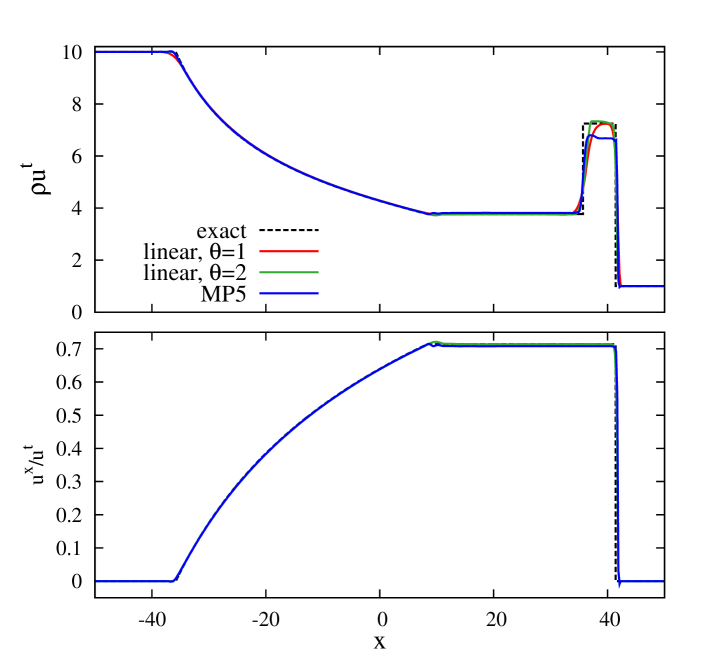
Figure 1: The relativistic shock tube test solved on 500 grid points using three reconstruction algorithms: slope-limited linear with $\theta=1$ (most diffusive, red), $\theta=2$ (green), and MP5 (blue). The black dotted line shows the exact solution for comparison.

This test shows that all the reconstruction schemes currently implemented in KORAL work reasonably well on relativistic hydrodynamic shocks. The MP5 scheme is most accurate in smooth regions, but it is also prone in some circumstances to give unphysical oscillations. The $\theta=1$ linear scheme is most diffusive, and at the same time is also the most stable. In the following tests, if not stated otherwise, we use the linear reconstruction scheme with $\theta=1.5$.

4.2 Polish doughnuts

To test the ability of the code to handle multi-dimensional hydrodynamics in curved spacetime, we set up analytical equilibrium torii (Polish doughnuts, Abramowicz et al., 1978) in the Schwarzschild metric as initial conditions and let the code evolve to a numerical equilibrium configuration. For the analytical model, we assume a constant specific angular momentum, $\ell=-u_{\phi}/u_{t}=$  constant. From the condition $u^{\mu}u_{\mu}=-1$, it follows that

$$u_{t}^{-2}=-g^{tt}+2\ell g^{t\phi}-\ell^{2}g^{\phi\phi}.$$ (62)

We choose the specific internal energy at the inner edge of the torus, $u_{t,\rm in}$, which determines the radius of the inner edge of the torus, and we then calculate the fluid enthalpy, $h=\rho+u+p$ (e.g., Hawley et al., 1984),

$$h=\frac{u_{t,\rm in}}{u_{t}}.$$ (63)

Using an equation of state $p=\kappa\rho^{\Gamma}$ (where the constant $\kappa$ determines the entropy of the torus gas), we obtain

$$\hskip 72.26999pt\rho = \left[\frac{(h-1)}{\kappa}\,\frac{(\Gamma-1)}{\Gamma}\right]^{1/(\Gamma-1)},$$ (64)

$$\hskip 72.26999ptu = \rho\,\frac{(h-1)}{\Gamma}.$$ (65)

We set the initial velocity to $v^{r}=v^{\theta}=0$, $v^{\phi}=u^{\phi}/u^{t}$, and choose $\Gamma=4/3$.

Table 2 gives parameter values corresponding to three models that we ran to test the code. Models 1 and 2 have the same value of the specific angular momentum, $\ell=4.5$. Model 1 has $u_{t,\rm in}=-1$, corresponding to a torus inner radius $r_{\rm in}=8$, while Model 2 has $u_{t,\rm in}=-0.98$, corresponding to $r_{\rm in}=10$. The specific angular momentum for the third model, $\ell=3.77$, lies in between the Keplerian values of $\ell$ at the marginally stable and marginally bound orbits ($\ell_{ms}<\ell<\ell_{mb}$). Therefore, this torus has a cusp (self-crossing equipotential surface) near the marginally bound orbit ($r_{mb}=4$). All the equipotential surfaces outside the body of the torus (defined by the critical surface producing the cusp) are open and continue into the BH. Therefore, the assumption of zero poloidal velocity cannot be applied to this region.

Table 2: Model parameters for Polish doughnuts tests

Model	$\ell$	$u_{\rm t,in}$	$\kappa$
1	4.5	-1.0	0.03
2	4.5	-0.98	0.03
3	3.77	-1.0	0.03

The above three torus models were simulated on a 50x50 grid in Boyer-Lindquist ($r$-$\theta$) coordinates, linearly spanning the range $r=3-27.8$ and $\theta=0-\pi/2$. At the spin axis and the equatorial plane, reflection boundary conditions were assumed. The analytical solution was imposed as boundary conditions in the ghost cells outside $r=27.8$. At the inner edge of the grid $r=3$, outflow boundary conditions were implemented. Linear reconstruction with $\theta=1.5$ was used.

Figure 2 compares the relaxed, stationary solutions obtained by running the code with the corresponding analytical Polish doughnut solution. Colors and orange solid lines show the numerical solution (density), while dashed green lines show the analytical model. Vectors indicate the poloidal component of velocity.

The top panel in Figure 2 corresponds to Model 1, where the analytical solution extends from $r=8$ to the outer boundary. The analytical and numerical contours agree very well. The only visible discrepancy is in the low-density region near the torus inner edge, where there is some numerical dissipation.

The middle panel in Figure 2 corresponds to Model 2, where the analytical torus is entirely confined within the grid: $r_{\rm in}=10$, $r_{\rm out}=27$. Again, the numerical solution agrees very well with the analytical solution except for the innermost region of the torus where the numerical solution is slightly stretched inward.

The bottom panel in Figure 2 shows Model 3. The analytical contours plotted correspond to open equipressure surfaces which intersect the BH horizon. Non-zero poloidal velocities are thus expected in this model and the analytical solution is not fully consistent. Nevertheless, there is a close similarity between the numerical and analytical solutions, which means that the code is able to represent even this torus quite well.

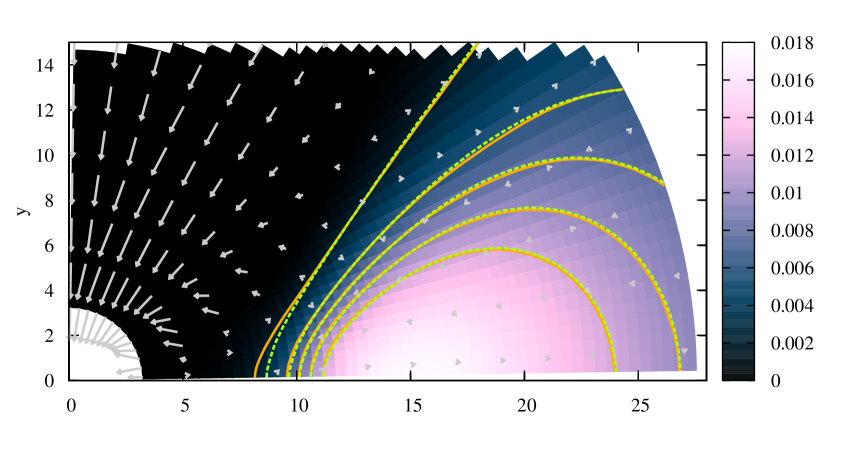
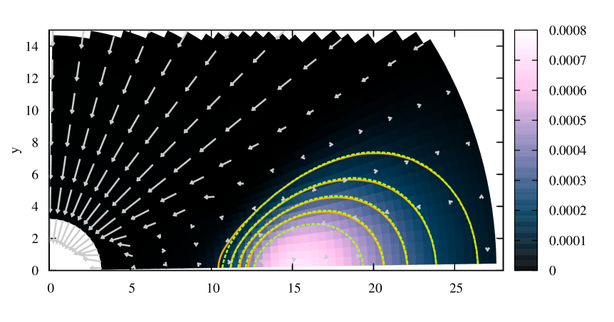
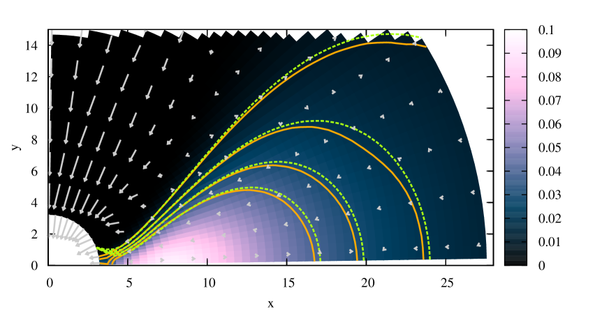
Figure 2: Equilibrium torii (Polish doughnuts) around a Schwarzschild BH after numerical evolution up to time $t=1000M$. Colors and arrows show density and poloidal velocity, respectively. The green dashed lines show iso-density contours of the analytical solutions. Contours for the numerical solutions are shown with orange solid lines. The parameters of the three model torii are given in Table 2.

4.3 Radiative shock tubes

The previous two tests did not involve radiation. For our first test with radiation, we set up a number of radiative shock tube problems as described in Farris et al. (2008) and Roedig et al. (2012). These shock tubes are similar to the pure hydrodynamic shock tube described in Section 4.1, i.e., the system begins with gas in two different states (left and right), separated by a membrane. The membrane is removed at $t=0$ and the system is allowed to evolve. The difference here is that the evolution is described by the full set of equations (23)–(25). In addition, the left- and right-states of all the tests except test No. 5 are set up in such a way that the shock asymptotically becomes stationary (see Appendix C of Farris et al., 2008).

Table 3 lists the parameters describing the initial states of seven test problems that we have simulated. The scattering opacity in all the tests is set to zero, so $\chi=\kappa$ (equation 18). The value of the radiative constant $\sigma$ in code units is given in the table. All the tests were solved on a grid of $800$ uniformly spaced points. For consistency with previous work by other authors, the Eddington approximation was used (equation 26).

Table 3: Radiative shock tubes

Test					Left state:					Right state:
No.	$\Gamma$	$\sigma$	$\kappa/\rho$		$\rho$	$p$	$u^{x}$	$\widehat{E}$		$\rho$	$p$	$u^{x}$	$\widehat{E}$
1	5/3	$3.085\cdot 10^{9}$	0.4		1.0	$3.0\times 10^{-5}$	0.015	$1.0\times 10^{-8}$		2.4	$1.61\times 10^{-4}$	$6.25\times 10^{-3}$	$2.51\times 10^{-7}$
2	5/3	$1.953\cdot 10^{4}$	0.2		1.0	$4.0\times 10^{-3}$	0.25	$2.0\times 10^{-5}$		3.11	$4.512\times 10^{-2}$	$8.04\times 10^{-2}$	$3.46\times 10^{-3}$
3a	2	$3.858\cdot 10^{-8}$	0.3		1.0	$6.0\times 10^{1}$	10.0	$2.0$		8.0	$2.34\times 10^{3}$	$1.25$	$1.14\times 10^{3}$
3b	2	$3.858\cdot 10^{-8}$	25.0		1.0	$6.0\times 10^{1}$	10.0	$2.0$		8.0	$2.34\times 10^{3}$	$1.25$	$1.14\times 10^{3}$
4a	5/3	$3.470\cdot 10^{7}$	0.08		1.0	$6.0\times 10^{-3}$	0.69	$0.18$		3.65	$3.59\times 10^{-2}$	$0.189$	$1.3$
4b	5/3	$3.470\cdot 10^{7}$	0.7		1.0	$6.0\times 10^{-3}$	0.69	$0.18$		3.65	$3.59\times 10^{-2}$	$0.189$	$1.3$
5	2	$3.858\cdot 10^{-8}$	1000.0		1.0	$6.0\times 10^{1}$	1.25	$2.0$		1.0	$6.0\times 10^{1}$	$1.10$	$2.0$

Figure 3 shows the numerical (solid) and analytical (dashed lines) solutions for radiative shock tube problem No. 1, which corresponds to a non-relativistic strong shock. The panels show (top to bottom) density, proper velocity, fluid-frame radiative energy density and fluid-frame flux, and may be directly compared (but for the flux which the other authors plot in the lab frame) to the corresponding figures and analytical solutions of (Farris et al., 2008; Zanotti et al., 2011; Fragile et al., 2012). The agreement is good.

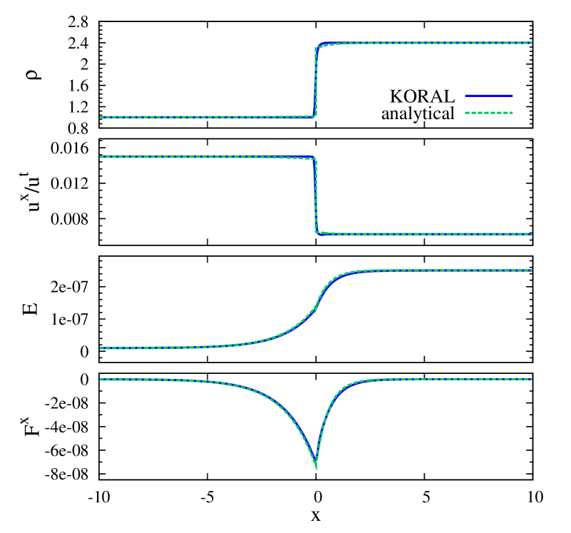
Figure 3: Results obtained for radiative shock tube test No. 1. From top to bottom, the panels show the profiles of gas density, proper velocity, fluid-frame radiative energy density and fluid-frame radiative flux. The numerical solution obtained with KORAL is indicated by solid lines and the semi-analytical solution given in Farris et al. (2008) by dotted lines.

Figure 4 shows results for radiative shock tube test No. 2, which corresponds to a mildly relativistic strong shock. Again, the agreement between the numerical and semi-analytical (Farris et al., 2008) profiles is good, except for a slight smoothing of the numerical profiles at the position of the shock (see the bottom panel).

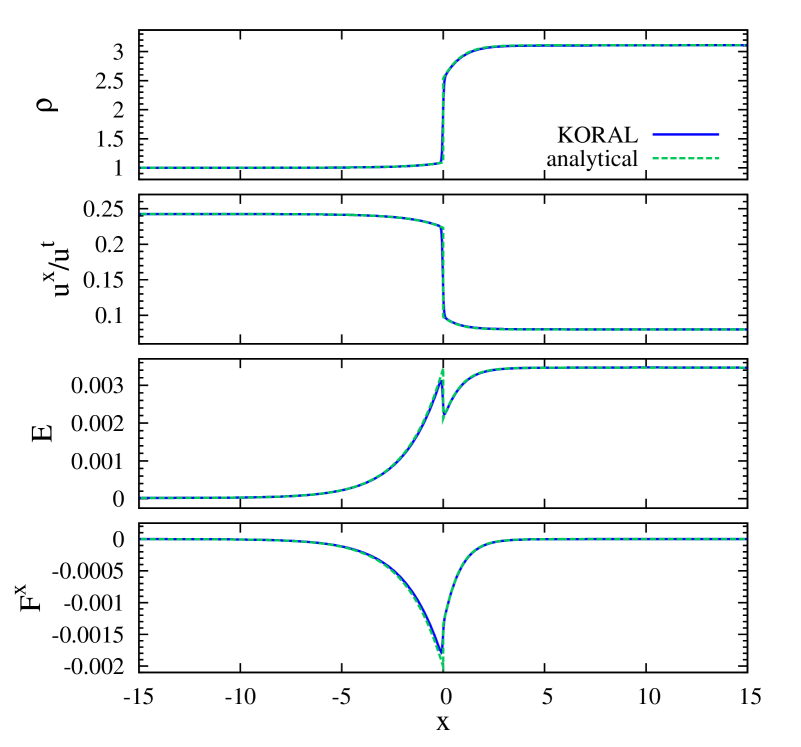
Figure 4: Same as Figure 3 but for radiative shock tube test No. 2.

Figure 5 shows results corresponding to radiative shock tube tests No. 3a and 3b. These are strongly relativistic shocks with upstream $u^{x}=10$. Test No. 3a corresponds to shock tube test 3 of Farris et al. (2008), while test 3b is the optically thick version of the same test which was proposed and solved by Roedig et al. (2012). These two tests verify that the code is able to resolve a highly relativistic wave in two very different optical depth limits. In both cases, the numerical solution reaches a steady state and closely follows the corresponding semi-analytical solution. The only noticeable difference is that in the high-opacity case the discontinuity in the numerical solution is less steep than in the exact analytical profile. This discrepancy measures the amount of numerical dissipation introduced by the algorithm.

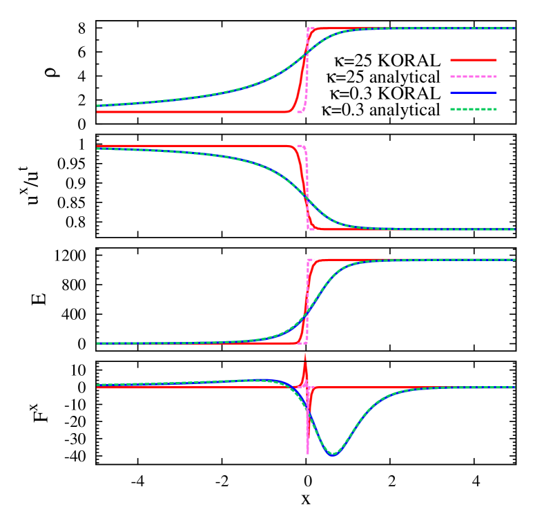
Figure 5: Similar to Figure 3 but showing results for radiative shock tube tests No. 3a (solid blue: numerical solution, dotted green: exact semi-analytical solution) and No. 3b (solid red: numerical, dotted magenta: semi-analytical).

Figure 6 shows results for radiative shock tube tests No. 4a and 4b. These tests correspond to radiation pressure dominated mildly relativistic waves. Test 4b is the optically thick version of test 4a that was proposed by Roedig et al. (2012). In both tests, the numerical solution reaches a stationary state and agrees well with the semi-analytical solution. Note that the values of the opacity coefficient $\kappa$ in tests 3b and 4b are the maximum values that the numerical scheme of Roedig et al. (2012) could handle. The algorithm implemented in KORAL has no such a limitation. We could increase $\kappa$ to much larger values and the scheme would remain stable.

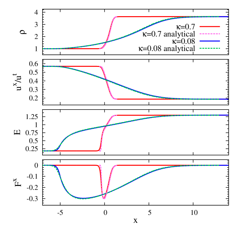
Figure 6: Similar to Figure 3 but showing results for radiative shock tube tests No. 4a (solid blue: numerical solution, dotted green: semi-analytical solution) and No. 4b (solid red: numerical, dotted magenta: semi-analytical).

Figure 7 corresponds to radiative shock tube test No. 5. This is the only test that does not asymptote to a stationary solution. This test was proposed and solved by Roedig et al. (2012) and represents an optically thick flow with mildly relativistic velocities. The left- and right-states are identical except that they have different velocities. As a result, two shock waves propagate in opposite directions. This test does not have an analytical solution. However, by comparing our numerical solution with that presented in Roedig et al. (2012), we confirm that our scheme performs satisfactorily.

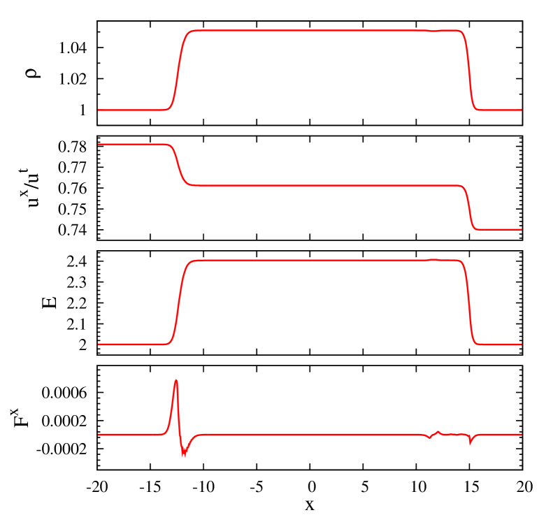
Figure 7: Same as Figure 3 but for radiative shock tube test No. 5. There is no analytical solution available for this problem.

4.4 Radiative pulse

We now test the ability of our scheme to handle the evolution of a radiation pulse in the optically thick and optically thin limits. We start with the optically thin case. We set up a Gaussian distribution of radiative energy density at the center of a 3D Cartesian coordinate system. The pulse radiative temperature is set according to,

$$T_{\rm rad}=\left(\frac{E}{4\sigma}\right)^{1/4}=T_{0}\left(1+100e^{-(x^{2}+y^{2}+z^{2})/w^{2}}\right),$$ (66)

with $T_{0}=10^{6}$, $w=5.0$ and the radiative constant $\sigma=1.56\times 10^{-64}$. We assume zero absorption opacity ($\kappa=0$) and non-zero but negligible scattering opacity ($\kappa_{\rm es}=10^{-6}$). The background fluid field has constant density $\rho=1$ and temperature $T=T_{0}$. We solve the problem in three dimensions on a coarse Cartesian grid of $51x51x51$ cells using the linear reconstruction with $\theta=2$.

The initial pulse in radiative energy density is expected to spread isotropically with the speed of light (optically thin medium) and to decrease inversely proportionally to the square of radius (energy conservation). Such behavior is visible in Fig. 8 showing the radiative energy distribution in the $z=0$ plane (top panels) and its cross-section along $y=z=0$ (bottom panels). The orange circles in the top set of panels show the expected size of the pulse. It is clear that the propagation speed of the pulse is consistent. This problem was solved on a relatively coarse Cartesian grid. This results in deviations from the perfectly spherical shape — the radiative energy density of the pulse along the axes is higher than along the diagonals. This effect is reduced by choosing larger resolution or a more suitable grid (e.g., spherical). The bottom set of panels in Fig. 8 shows the profiles of the energy density along the $x$-axis. The black dotted lines show the expected rate of energy decrease with increasing distance from the center. The numerical solution perfectly follows this trend.

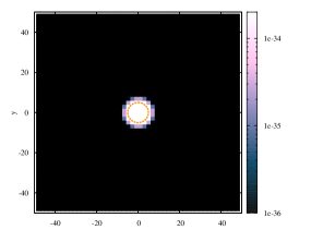
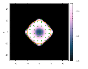
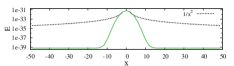
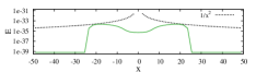
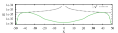
Figure 8: Profiles of the radiative energy density ($E$) for the optically thin radiative pulse test described in Section 4.4. The top panels show its distribution in the $xy$ plane at (from left to right) $t=0$, $15$ and $35$. The orange circle in the first plot denotes the initial width and expands at the speed of light to provide the expected pulse front location in the other two plots. The bottom panels show the corresponding profiles measured along $y=z=0$ line and the $1/x^{2}$ dependence

To test the optically thick limit we choose to set up a similar pulse but this time planar instead of a point-like, i.e., according to,

$$T_{\rm rad}=\left(\frac{E}{4\sigma}\right)^{1/4}=T_{0}\left(1+100e^{-x^{2}/w^{2}}\right).$$ (67)

This time we set the scattering opacity to $\kappa_{\rm es}=10^{3}$ and solve the problem as one-dimensional on $101$ grid points distributed uniformly between $x=-50$ and $x=50$ with periodic boundary conditions in $y$ and $z$. The total optical depths per cell and per pulse are therefore $\tau=10^{3}$ and $\tau=10^{4}$, respectively.

In the optically thick limit the evolution of such a system is described by a diffusion equation,

$$\partial_{t}E=\frac{1}{3\chi}\partial_{xx}E,$$ (68)

which can be derived from the non-relativistic limit of Eq. 25 assuming the time derivative of the $x$ component of the flux vanishes. An initially Gaussian pulse of radiative internal energy will therefore diffuse according to the value of the diffusion coefficient $1/3\chi$.

In Fig. 9 we plot profiles of the radiative energy at various moments (solid lines) and compare them to the exact solution of Eq. 68 (dotted lines). The numerical solution diffuses slightly faster due to the additional numerical dissipation introduced by the scheme. At later times this difference becomes insignificant.

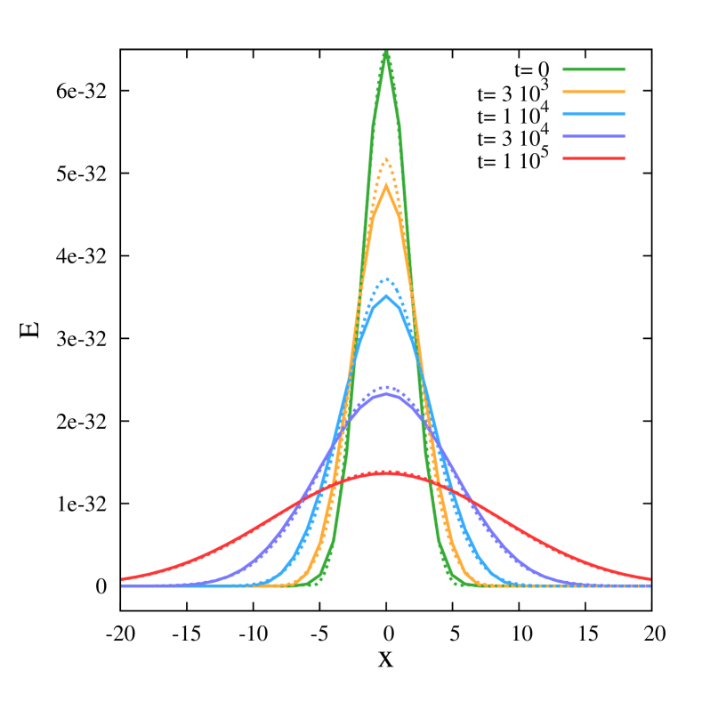
Figure 9: The radiative energy density for the optically thick pulse described in Section 4.4. The green line shows the initial profile while the other color show the time evolution. Dotted lines show the exact solution of Eq. 68.

4.5 Shadow test

Here we test the ability of the M1 closure scheme, as incorporated in KORAL, to resolve shadows. We set up a blob of dense, optically thick gas in flat spacetime, surrounded by an optically thin medium, and we illuminate this system.

We start with a single source of light imposed on the left boundary. We solve the problem in two dimensions on a 100x50 grid, with the density distribution set to be

$$\rho=\rho_{0}+(\rho_{1}-\rho_{0})\,e^{-\sqrt{x^{2}+y^{2}}/w^{2}},$$ (69)

where $\rho_{0}=10^{-4}$, $\rho_{1}=10^{3}$ and $w=0.22$. The gas temperature is adjusted so as to give constant pressure throughout the domain,

$$T=T_{0}\frac{\rho}{\rho_{0}}.$$ (70)

The initial radiative energy density is set to the local thermal equilibrium value, and the initial velocities and radiative fluxes are zero. We apply periodic boundary conditions at the top and bottom and outflow boundary conditions at the right border of the domain. At the left border we have the external source of light, which we specify with $E_{L}=4\sigma T_{L}^{4}$, $F^{x}=0.99999E_{L}$, $T_{L}=100T_{0}$. All other quantities are set to match the ambient gas. We evolve the system with both the Eddington approximation and M1 closure, assuming $\kappa=\chi=\rho$.

Figure 10 shows the results at $t=10$. By this time, the initial radiation wave has passed through the domain and the system has reached a stationary state. The upper panel shows the solution we obtain with the Eddington approximation. Because this closure treats all directions equally, radiation readily diffuses into the region behind the blob. As a result, there is no shadow behind the optically thick blob. The lower panel in Figure 10 shows results with the the M1-closure. In contrast to the case of Eddington closure, here the $x$ direction is distinguished because the incoming radiation at the left boundary moves in this direction. The M1 closure is designed to keep flux moving parallel to itself in optically thin regions for $F\approx E$. As a result, a strong shadow develops behind the optically thick blob. This test illustrates one of the key differences between the Eddington and M1 closure schemes.

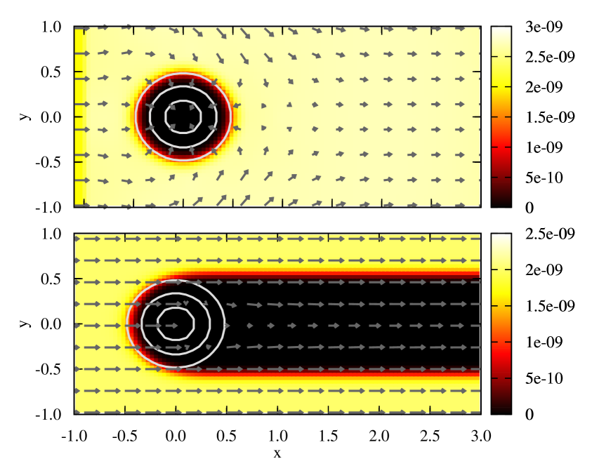
Figure 10: Results obtained with the shadow test for a single beam of light. The upper panel corresponds to the Eddington approximation and the lower panel to the M1 closure scheme. Colors denote radiative energy density, contours show density ($\rho=1$, $100$, $500$) and arrows show the direction and magnitude of the reduced radiative flux $F^{i}/E$.

It is appropriate to mention that the excellent performance of the M1 closure scheme in this shadow test problem is partly because the setup is particularly favorable. First, we have only a single source of radiation. Second, the shadow here is aligned well with the grid, which helps to minimize diffusion. For other grid orientations, the numerical results would exhibit more diffusion, e.g., see Section 4.7.

The M1 closure assumes that the specific intensity is symmetric with respect to the radiative flux, i.e., only one direction is distinguished. It means that this approach is supposed to be less efficient when multiple sources of light are involved. To test its performance for such a setup we implemented a two-beam test problem similar to the one described in Jiang et al. (2012). We set up exactly the same initial conditions for gas and radiation as in the two previous tests. This time, however, we set up a reflection symmetry at the lower boundary ($y=0$) and we impose an inclined ($F^{x}_{0}=0.93E_{0}$, $F^{y}_{0}=-0.37E_{0}$) beam on the upper boundary and on the part ($y>.3$) of the left boundary. As a result, the domain is effectivelly enlighted by two self-crossing beams of light. We plot the result of a numerical simulation in Fig. 11 where the region of negative $y$-coordinates was plotted by reflecting the $y$-positive data. In the region near the left top and bottom corners, where the beams do not overlap, the direction of the flux follows the imposed boundary condition. In the region of the overlap the radiative energy density increases twice ($E=2E_{0}$) while the flux becomes equivalent to the superposition of the beam-intrinsic fluxes, i.e., it is purely horizontal and its $x$-component equals $F^{x}=2F^{x}_{0}=1.86E_{0}=0.93E$. The clump of optically thick gas is, therefore, effectively illuminated by a purely horizontal beam. One could expect it creates a parallel shadow similar to the one obtained in the single beam problem. This is, however, not the case. There is an important difference between the beam we imposed on the left boundary in the single beam problem and the one which develops in the overlapping region. The former had $F^{x}\approx E$ what implied that the specific intensity was almost a $\delta$ function in the direction of the flux. The latter, however, has $F^{x}=0.93E$ which means that the implied distribution of the specific intensity is only an elongated ellipsoid pointing in the direction of the flux, i.e., photons moving in other directions than the direction of the flux are allowed. This has an effect on the shadow produced behind the clump. Instead of sharp parallel edges we get regions of the partial shadow (penumbra) resulting from these perpendicular photons allowed by the closure when $F^{x}<E$. The region of the total shadow (umbra) is therefore limited by the edges of the penumbra and follows the expected shape (compare Fig. 11 in Jiang et al. (2012)) to a good accuracy. A significant difference between the exact solution and our numerical one arises in the region where the penumbrae overlap. One could expect a uniform, triangular region of no shadow. The M1 closure, however, produces an extra narrow horizontal shadow along the $x$-axis.

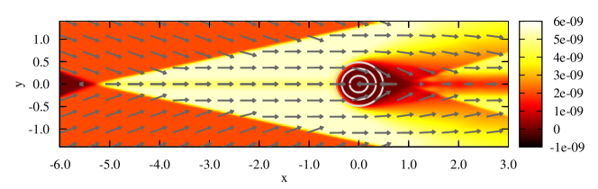
Figure 11: Similar to Fig. 10 but for two inclined beams of light.

This test shows limits of the M1 closure approach but at the same time stresses the fact that, in principle, it does not limit specific intensity to one particular direction (assuming only its symmetry with respect to the flux). It performs much better than the Eddington approximation but in the case of multiple sources of light it must be used with caution.

4.6 Static atmosphere

An important aspect of radiation in accretion disks is momentum transfer between radiation and gas. The Eddington luminosity limit, for instance, arises from this interaction. To validate the treatment of gas-radiation momentum exchange in our method, we study a static atmosphere which is in equilibrium under the combined action of gravity, gas pressure gradient and radiation force. We consider a polytropic atmosphere on a spherical object. We take the optically thin limit and assume that gas-radiation interactions occur only through a scattering coefficient, i.e., $\kappa=0$, $\chi=\kappa_{\rm es}$ (equation 18).

An analytical solution is easily derived for this model problem. Because we assume a polytropic equation of state and set $\kappa=0$, there is no energy equation, and the radial component of the momentum equation ($r$ component of equation 24) is all that matters. In the non-relativistic limit ($r\gg 2$), assuming stationarity ($\partial_{t}=0$) and zero velocity ($v^{i}=0$), this equation takes the form

$$\frac{1}{\rho}\frac{\partial p}{\partial r}=-\frac{1-f}{r^{2}},$$ (71)

where

$$f=\kappa_{\rm es}F_{\rm in}r_{\rm in}^{2}.$$ (72)

Here $F_{\rm in}$ is the radiative flux imposed as a boundary condition at the bottom of the atmosphere, $r=r_{\rm in}$, and $f$ gives the ratio of the radiative to gravitational (or geometrical) forces; $f=1$ corresponds to the Eddington limit, where the luminosity is $L_{\rm Edd}=4\pi/\kappa_{\rm es}$ and the radiative flux is $F_{\rm in}=F_{\rm Edd}=1/\kappa_{\rm es}r_{\rm in}^{2}$. Since radiative energy must be conserved, in the stationary state the flux must satisfy $F=F_{\rm in}r_{\rm in}^{2}/r^{2}$ (non-relativistic limit).

Equation (71) may be solved with the help of the polytropic equation of state $p=K\rho^{\Gamma}$ to give,

$$\rho=\left[\frac{(\Gamma-1)}{\Gamma K}\left(C+\frac{1-f}{r}\right)\right]^{\frac{1}{\Gamma-1}},$$ (73)

where

$$C=\frac{\Gamma K}{(\Gamma-1)}\rho_{\rm in}^{\Gamma-1}-\frac{1-f}{r_{\rm in}},$$ (74)

and $\rho_{\rm in}$ is the assumed density at $r=r_{\rm in}$. The entropy constant $K$ is calculated at the bottom of the atmosphere from the assumed gas temperature $T_{\rm in}$.

We set up a linear grid of $40$ points between $r=10^{6}$ and $1.4\times 10^{6}$ gravitational radii and we solved the problem using MP5 reconstruction scheme and the standard M1 closure. We scaled all quantities to physical units assuming $M=1M_{\odot}$ and $\kappa_{\rm es}=0.4\rho\,{\rm cm^{-1}}$. At the innermost radius we set $\rho_{\rm in}=10^{-15}\,{\rm g\,cm^{-3}}$ (optically thin atmosphere) and $T_{\rm in}=10^{6}\,\rm K$. All the velocities were initially zero and the radiative energy density $E=F_{\rm in}/0.99$. Initial values of the gas density and temperature in the domain and in the ghost cells were assigned based on the analytical solution. We ran four models corresponding to four luminosities: $10^{-10}$, $0.1$, $0.5$ and $1.0\,L_{\rm Edd}$. Each model was run up to a time $t=2\times 10^{9}M$, which is sufficient to reach relaxed steady state for these optically thin atmospheres.

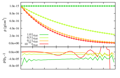
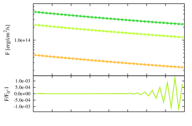
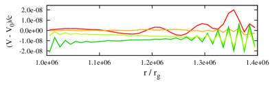
Figure 12: Results obtained with the static atmosphere test. Numerically determined profiles and residuals between the numerical and analytical solutions are plotted for the density (top panel), radial flux (middle panel) and radial velocity (bottom panel, residuals only). Colors denote the Eddington ratio of the flux boundary condition $F_{\rm in}$ at the bottom of the atmosphere: $F_{\rm in}=10^{-10}F_{\rm Edd}$ (red), $0.1F_{\rm Edd}$ (orange), $0.5F_{\rm Edd}$ (light green) and $1.0F_{\rm Edd}$ (dark green) Circles correspond to the numerical solutions and lines show the analytical profiles (equation 71).

Figure 12 shows the results. The top panel shows the density profiles corresponding to the four models. Solid lines are the analytical solutions and filled circles correspond to the numerical solutions. The agreement is very good. The higher the luminosity, the flatter is the density profile, indicating the effect of the outward force due to radiation. For the particular case of the Eddington luminosity, the density is perfectly constant, reflecting the fact that the gravitational force is exactly balanced by radiation and no pressure gradient in required. We see that the relaxed numerical solution is indistinguishable from the analytical solution, confirming that KORAL properly handles gas-radiation momentum exchange. The plot of residuals at the bottom of the panel indicates that fractional deviations in the density are below $10^{-4}$. Even this small discrepancy is at least in part because we are comparing a numerical solution from a GR code with an analytical solution derived under Newtonian physics.

The middle panel in Figure 12 shows our results for the radial radiative flux. Once again, the models behave very well and the agreement with the analytical solution is excellent. Finally, the bottom panel shows the residual radial velocities ($v_{r}/c$). These are of the order of $10^{-8}$ (they should be zero), and appear to be mostly driven by slight inconsistencies near the boundaries (possibly again because of a slight tension between GR and Newtonian physics).

4.7 Beam of light near BH

To test the performance of the code for radiation in strong gravitational field, we study propagation of a beam of light in the Schwarzschild metric. We consider three models, in each of which a beam of light is emitted in the azimuthal direction at a different radius. We decouple gas and radiation by neglecting absorptions and scatterings ($\kappa=\chi=0$). We run the models on a two-dimensional grid with 30 points distributed uniformly in $r$ between $r_{\rm in}$ and $r_{\rm out}$ (see Table 4 for values) and 60 points distributed uniformly in azimuthal angle $\phi$ between $\phi=0$ and $\pi/2$. Initially, we assign negligibly small values for all primitive quantities, including the radiation energy density and flux. We use outflow boundary conditions on all borders except the region covered by the beam at the equatorial plane (see the range of $r_{\rm beam}$ in Table 4), where we set the radiation temperature to $T_{\rm beam}=10^{10}=1000T_{0}$ and the flux to $F^{\phi}=0.99999E$. Here $T_{0}$ is the initial gas and radiation temperature of the ambient medium. We use linear reconstruction with $\theta=1$.

Table 4: Model parameters for the light beam tests

Model	$r_{\rm beam}$	$r_{\rm in}$	$r_{\rm out}$
1	$3.0\pm 0.1$	2.5	3.5
2	$6.0\pm 0.2$	5.3	7.5
3	$16.0\pm 0.5$	14.0	20.5

The panels in Figure 13 show the results for the three models and geodesics of photons at beam boundaries. Consider the right panel, which corresponds to Model 3 (Table 4) with the beam centered at $r_{\rm beam}=16$. At such a large radius we do not expect significant bending of photon geodesics and this is indeed the case — the beam is only slightly bent towards the BH. We also expect the beam to be tighly confined, i.e., it should propagate with a nearly constant width, as indicated by the two solid green lines, the true geodesics of photons at the boundaries of the beam. However, the numerical solution shows significant artificial broadening. This is caused by numerical diffusion which is significant whenever the radiative flux vector is not aligned with the grid geometry, i.e., the beam is tilted with respect to the grid axes.

The middle panel in Figure 13 shows Model 2, where the beam is centered at the marginally stable orbit: $r_{\rm beam}=6$. At this radius, photon geodesics are significantly deviated by gravity, resulting in strong curvature in the beam. The numerical beam follows the correct trajectory. Moreover, numerical diffusion is lower in this case because the curvature brings the beam into closer alignment with the grid. There is in addition some real beam divergence because the geodesics at different radii within the beam have different curvatures (see the solid green lines), but this effect is not very significant.

Finally, the left panel in Figure 13 shows Model 1, where the center of the beam is exactly at the photon orbit: $r_{\rm beam}=3$. An azimuthally oriented ray at this radius is expected to orbit around the BH at a constant $r$. This is seen clearly in the numerical solution. Moreover, since the photon geodesic follows the grid, there is practically no numerical diffusion. Indeed, there is less diffusion than there should be (compare the numerical beam with the two solid green lines). The beam should have some divergence as it propagates around the BH because photons emitted inside $r=3$ curve inward and will ultimately fall into the BH, while those emitted outside $r=3$ curve outward and will move towards infinity. The simulated beam does not reproduce this physical broadening very well.

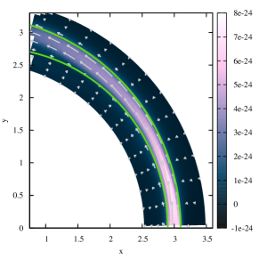
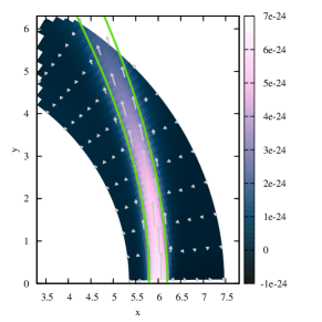
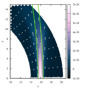
Figure 13: Results for Model 1 (left panel), Model 2 (middle), Model 3 (right), involving light beams propagating near a Schwarzschild BH (see Table 4 for model details). The BH is at $r=0$ (i.e., $x=y=0$). The beams are introduced via a boundary condition on the $x$-axis. The beams initially move vertically, i.e., in the azimuthal direction. Color indicates the radiation energy density and arrows show the radiative flux as measured by a ZAMO. The solid green lines indicate true geodescis of photons at the beam boundaries. They were calculated using the ray-tracing code GYOTO (Vincent et al., 2011).

4.8 Radiative spherical accretion

Our last test problem considers radiative spherical accretion onto a non-rotating BH. This problem has been studied in the past by Vitello (1984) and Nobili et al. (1991) and more recently by Roedig et al. (2012) and Fragile et al. (2012). We follow Fragile et al. (2012) in the setup of our simulations to facilitate comparison with their results. As in their work, we consider Thomson scattering and thermal bremsstrahlung, which give the following opacity coefficients,

$$\hskip 50.58878pt\kappa = 1.7\times 10^{-25}T^{-7/2}m_{p}^{-2}\rho\,{\rm cm^{-1}},$$ (75)

$$\hskip 50.58878pt\chi = \kappa+0.4\rho\,{\rm cm^{-1}},$$ (76)

where $\rho$ is in ${\rm g\,cm^{-3}}$ and $m_{p}$ is the mass of the proton. Our numerical grid spans from $r_{\rm in}=2.5$ to $r_{\rm out}=2\times 10^{4}$ and is resolved by 512 grid points spaced logarithmically following $x=\log\left((r-2.2)/2\right)$ where the auxiliary variable $x$ is spaced linearly between values corresponding to $r_{\rm in}$ and $r_{\rm out}$. We assume a BH mass of $3M_{\odot}$. For the initial state, we choose the mass accretion rate $\dot{M}$ (see Table 5 for values) and set the density profile accordingly,

$$\rho=-\frac{\dot{M}}{4\pi r^{2}u^{r}},$$ (77)

where the radial velocity $u^{r}$ is equal to its free fall value $u^{r}=-\sqrt{2/r}$. The gas temperature is given by

$$T=T_{\rm out}\left(\frac{\rho}{\rho_{\rm out}}\right)^{\Gamma-1},$$ (78)

where $T_{\rm out}$ is the temperature at the outer radius and $\Gamma$ is the adiabatic index. The latter is calculated from the radiation to gas pressure ratio $f_{p}=p_{\rm rad}/p_{\rm gas}$ of the initial state (Table 5),

$$\Gamma=1+\frac{1}{3}\left(\frac{2+2f_{\rm p}}{1+2f_{\rm p}}\right).$$ (79)

The radiative energy density is set to $E=3f_{\rm p}p_{\rm gas}$.

The numerical simulations are run in one (radial) dimension with the MP5 reconstruction scheme, and M1 closure for the radiation. The primitive quantities at the outer boundary are fixed at their initial values, as described above. At the inner boundary we apply outflow boundary conditions, with the radial velocity fixed at the free-fall value and rest mass density and internal energy extrapolated proportional to $r^{-3/2}$ and $r^{-3/2\Gamma}$, respectively. Table 5 lists the parameter values we used corresponding to five models. The first model, E1T6, is characterized by the lowest mass accretion rate and is designed to highlight the ability of our scheme to handle optically thin media. The other four models are identical to simulations described in Fragile et al. (2012).

Table 5: Models parameters for radiative spherical accretion tests

Model	$\dot{M}/\dot{M}_{\rm Edd}$	$T_{0}[K]$	$f_{\rm p}=\frac{p_{\rm rad}}{p_{gas}}$	$L/L_{\rm Edd}$
E1T6	1.0	$10^{6}$	$1.2\times 10^{-4}$	$8.73\times 10^{-8}$
E10T5	10.0	$10^{5}$	$1.2\times 10^{-7}$	$3.26\times 10^{-6}$
E10T6	10.0	$10^{6}$	$1.2\times 10^{-4}$	$6.51\times 10^{-6}$
E10T7	10.0	$10^{7}$	$1.2\times 10^{-1}$	$1.45\times 10^{-5}$
E100T6	100.0	$10^{6}$	$1.2\times 10^{-4}$	$2.00\times 10^{-4}$

Model names and parameters after Fragile et al. (2012).

Figure 14 shows the numerical solutions obtained with KORAL. The top-left panel presents profiles of density, which follow the initial profile (equation 77) throughout the simulation. The bottom-left panel shows the gas temperature. For all but the coldest model, E10T5, the temperature follows equation (78). In the case of model E10T5, the gas is hotter than the analytical result. This is because of gas-radiation coupling which heats up the gas as it approaches the BH (the analytical solution assumes that there is no interaction). The small kinks in the temperature profiles near the inner boundary are an artifact of the inner boundary condition. They do not influence the rest of the solution since information cannot travel upstream in the supersonic flow.

The top-right and bottom-right panels in Figure 14 show radial profiles of the radiative energy density and flux for the five models. Both quantities follow roughly an $r^{-2}$ scaling, reflecting the fact that in steady-state (barring redshift factors) the luminosity is equal to $4\pi Fr^{2}$ and should be conserved.

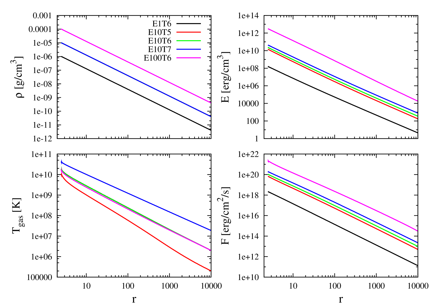
Figure 14: Numerical results obtained with KORAL for five models of spherical Bondi accretion with radiation. The panels show density (top-left), radiative energy density (top-right), gas temperature (bottom-left) and radiative radial flux (bottom-right). Parameters of the models are given in Table 5. The results show that the code handles optically-thin and optically-thick regions equally well, without producing unphysical oscillations.

Because the flux in these models is non-negligible compared to the energy density (e.g., $F\approx 0.9E$ for the E10 family of models), the Eddington closure scheme does not work very well, especially at low optical depth. For instance, Fragile et al. (2012) used Eddington closure and obtained unphysical noise or breaks in their profiles of radiative quantities (see their Figure 5) in all models with $\dot{M}<300\dot{M}_{\rm Edd}$. This just reflects the fact that their closure cannot handle optically thin media. Our algorithm uses the M1 closure scheme and has no problems with either optically thick or thin regimes. To emphasize this point, we have solved an additional model, E1T6, in which the accretion rate is an order of magnitude lower than the smallest rate considered by Fragile et al. (2012). KORAL works fine for this model, and can, in fact, handle even more extreme configurations, both at lower and higher accretion rates.

For direct comparison of our results with those reported in Fragile et al. (2012), we have calculated for all our models the luminosities,

$$L=4\pi Fr^{2},$$ (80)

emerging at radius $r=10^{3}$. Our results, shown in Figure 15, are consistent with those obtained by Fragile et al. (2012) (compare their Figure 6). Note, however, an important difference. The scheme used by Fragile et al. (2012) is explicit, therefore it cannot reliably treat optically-thin media. This causes the luminosities they quote to be sensitive to the radius at which they are measured. For instance, reading off the luminosity values in their simulations (Figure 5 of their paper) at a distance at which the flow is optically thin, e.g., $r=10^{4}$, one obtains erroneous lower values of the luminosity.

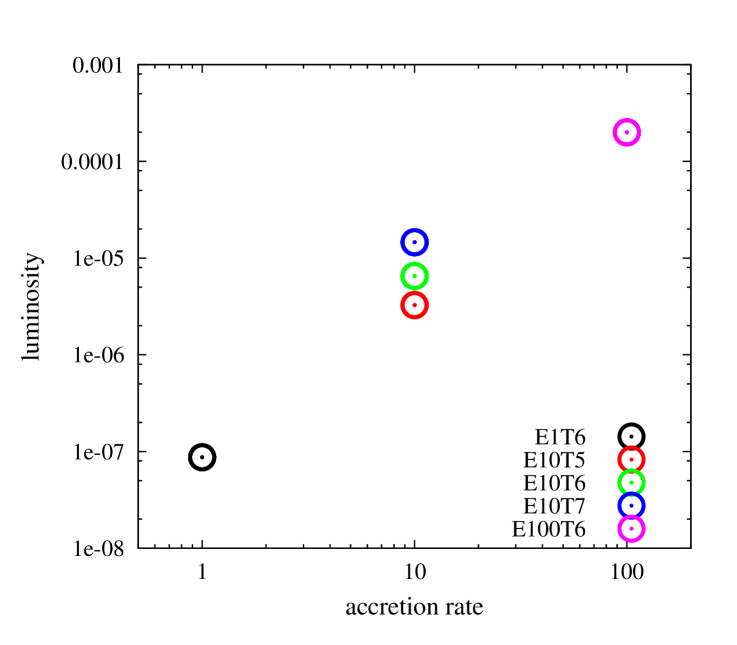
Figure 15: Luminosity (in Eddington units) emerging from a spherically symmetric radiative Bondi accretion flow onto a non-rotating BH, plotted as a function of the dimensionless (reduced) accretion rate in units of the Eddington accretion rate, $\dot{M}/\dot{M}_{\rm Edd}$. Parameters of the models are given in Table 5. Low accretion rates, where the accretion flow becomes optically thin, are usually problematic for numerical codes. KORAL has no problem handling either low or high accretion rates.

5 Summary

In this paper we have introduced a semi-implicit numerical scheme for general relativistic radiation hydrodynamics. The scheme is based on a covariant formulation of the M1 closure scheme for the radiation moments. The radiative source terms are handled semi-implicitly, and hence this approach can handle practically all optical depths. The algorithm has been implemented and tested in a new GRRHD code KORAL. It can be easily incorporated into any general relativistic hydrodynamic or magnetohydrodynamic conservative code.

Our tests indicate that KORAL works well for a variety of physical regimes and geometries: optically thick vs optically thin, gas dominated vs radiation dominated, flat space vs curved space. Also, as expected, we find that M1 closure has some advantages over the standard Eddington closure scheme in the case of optically-thin media: namely, it accurately propagates light rays and it is able to resolve shadows.

The semi-implicit radiation scheme implemented in KORAL does not overwhelmingly slow down the code. Apart from the fact that the inclusion of radiation introduces 4 new conserved quantities compared to pure hydrodynamics, the only important computational steps that affect performance are (i) calculation of the radiative characteristic wavespeeds (Section 3.2), and (ii) numerical solution of the system of four non-linear equations that arise in the implicit treatment of radiative source terms (Section 3.3). We expect each of these steps could be speeded up with more effort. However, even without further improvements, the code performance is already sufficiently good that global GRRHD or GRRMHD simulations of accretion disks with near- or super-Eddington luminosities appear feasible. Meanwhile, it would be of great interest to develop closure schemes beyond M1, e.g., by directly evolving the photon distribution function and using it to close the radiation moments, for conservative GR codes.

6 Acknowledgements

The authors thank Frederic Vincent for calculating the photon trajectories shown in Fig. 13, James M. Stone for insightful discussions, and the referee for helpful comments. RN and AS were supported in part by NASA grant NNX11AE16G. AT was supported by the Princeton Center for Theoretical Science Fellowship. We acknowledge NSF support via XSEDE resources, NICS Kraken and Nautilus under grant numbers TG-AST080026N (RN and AS) and TG-AST100040 (AT), and NASA support via High-End Computing (HEC) Program through the NASA Advanced Supercomputing (NAS) Division at Ames Research Center (AS and RN) that provided access to the Pleiades supercomputer.

Appendix A Explicit-implicit method for the radiative source operator

In Sect. 3.3 we described a semi-implicit method for applying the radiative source terms $G^{\mu}$ in the lab frame. It requires solving a four-dimensional system of non-linear equations. Because of that fact, the numerical efficiency is limited. Furthermore, the method may sometimes fail to produce a solution, e.g., when the initial guess is not close enough to the true solution or when the solution at an intermediate iteration becomes unphysical such as having $\widehat{F}>c\widehat{E}$. To handle these situations we have developed the approximate analytical method described in this Appendix, which is both robust and failsafe. We use it as a backup solver for the fiducial algorithm. Its limitations are discussed below.

Let us assume that the advective and geometric source terms have already been applied as per steps (i)–(ix) in Section 3.1. The only remaining terms are the radiative forces. For instance, equations (25) require us to time-evolve

$$\partial_{t}(R^{t}_{\nu})=-G_{\nu}.$$ (81)

Let us assume to start with that we treat this term explicitly. Then, the update of the conserved quantities is given simply by

$$\Delta R^{t}_{\nu}=-G_{\nu}\Delta t.$$ (82)

The right hand side can be rewritten as

$$-G_{\nu}\Delta t=-g_{\mu\nu}G^{\mu}\Delta t=-g_{\mu\nu}\Lambda^{\mu}_{\alpha}\widehat{G}^{\alpha}\Delta t,$$ (83)

where $\widehat{G}^{\alpha}$ is the radiative four-force in the fluid frame.

In the same explicit spirit, the fluid-frame source terms in equations (44) may be written as

$$\hskip 86.72377pt\Delta\widehat{E} = -\widehat{G}^{t}\Delta t,$$ (84)

$$\hskip 86.72377pt\Delta\widehat{F}^{j} = -\widehat{G}^{j}\Delta t.$$

These updates of $\widehat{E}$ and $\widehat{F}^{j}$ generally do not correspond to the updates of the conserved quantities we search for because the spatial and temporal derivatives are mixed when moving from one frame to another, i.e., the operator splitting is frame-dependent. However, comparing the right hand sides of equations (83) and (84), it is clear that the change in the conserved quantities is related to the updates of the primitive radiative quantities $\widehat{E}$ and $\widehat{F}^{i}$ calculated purely in the fluid frame. From equations (82) and (83) it follows that

$$\Delta R^{t}_{\nu}=g_{\mu\nu}\Lambda^{\mu}_{\alpha}\widehat{\Delta}_{P}^{\alpha},$$ (85)

where components of the four-vector of updates of primitive radiative quantities in the fluid frame, $\widehat{\Delta}_{P}$ (calculated according to equation 84), are given by the following 4-vector,

$$\widehat{\Delta}_{P}=[\Delta\widehat{E},\Delta\widehat{F}^{j}].$$ (86)

This quantity may be found using either explicit or implicit methods.

The explicit approach is the simplest and fastest in the optically thin regime, but it fails in the optically thick regime. To calculate $\widehat{\Delta}_{P}$ via the explicit approach, we simply set

$$\widehat{\Delta}_{P}=[-\widehat{G}^{t}_{(n)}\Delta t,-\widehat{G}^{j}_{(n)}\Delta t],$$ (87)

where the subscript $(n)$ indicates variables evaluated at the beginning of the current time step.

The implicit approach works well for all optical depths, and is especially important at high optical depths, but it usually involves more computations. In principle, one should solve the following set of fluid-frame equations for gas internal energy, momenta, radiative energy and fluxes,

$$\hskip 28.90755ptu_{(n+1)}-u_{(n)} = \kappa(\widehat{E}_{(n+1)}-4\sigma T^{4}_{(n+1)})\Delta t,$$ (88)

$$\hskip 28.90755ptm^{j}_{(n+1)}-m^{j}_{(n)} = \chi\widehat{F}^{j}_{(n+1)}\Delta t,$$ (89)

$$\hskip 28.90755pt\widehat{E}_{(n+1)}-\widehat{E}_{(n)} = -\kappa(\widehat{E}_{(n+1)}-4\sigma T^{4}_{(n+1)}),$$ (90)

$$\hskip 28.90755pt\widehat{F}^{j}_{(n+1)}-\widehat{F}^{j}_{(n)} = -\chi\widehat{F}^{j}_{(n+1)}\Delta t,$$ (91)

where the subscripts $(n)$ and $(n+1)$ denote values at the beginning and the end of the current time step, respectively, and $\kappa$ and $\chi$ are computed from the gas properties at time $(n+1)$. As a simplification, we assume that $\kappa$ and $\chi$ do not change significantly during a single time step, and we set

$$\hskip 86.72377pt\kappa = \kappa(\rho,T_{(n)}),$$ (92)

$$\hskip 86.72377pt\chi = \chi(\rho,T_{(n)}).$$ (93)

Now, equation (91) becomes decoupled from the others and may be solved directly for the updated fluxes,

$$\widehat{F}^{j}_{(n+1)}=\frac{\widehat{F}^{j}_{(n)}}{1+\chi\Delta t}.$$ (94)

To find the new value of the radiative energy density one has to solve equations (88) and (90) together. Taking into account the ideal gas equation of state,

$$p=(\Gamma-1)u=\frac{\cal R}{\mu}\rho T,$$ (95)

where $\mu$ is the mean molecular weight, it is straightforward to combine these two equations into one quartic equation for $\widehat{E}_{(n+1)}$. KORAL solves this equation numerically using the Newton method with $\widehat{E}_{(n)}$ as the initial guess. However, analytical solvers for quartic equations may also be implemented; in fact, a linearized version of the quartic is often quite adequate. Once $\widehat{E}$ and $\widehat{F}^{j}$ have been calculated, the four-vector of updates, $\widehat{\Delta}_{P}$, is given by,

$$\widehat{\Delta}_{P}=[\widehat{E}_{(n+1)}-\widehat{E}_{(n)},\widehat{F}^{j}_{(n+1)}-\widehat{F}^{j}_{(n)}].$$ (96)

This update is applied in step (xi) of the algorithm (see Section 3.1) in case the fiducial lab frame implicit method fails.

The updates of the conserved quantities calculated using this approach diverge from the fiducial semi-analytical results in the limit of large velocites $u^{t}\gg 1$ and large optical depths per cell $\tau\gg 1$. Therefore, in general, one should use this algorithm only as a failsafe backup method. However, if one is confident that the problem at hand does not involve such conditions, one might consider using this method as the default, thereby increasing the code efficiency.

References

- Abramowicz et al. (1995) Abramowicz, M. A., Chen, X.-M., Kato, S., Lasota, J.-P., & Regev, O. 1995, Astrophysical Journal, 438, L37
- Abramowicz et al. (1988) Abramowicz, M. A., Czerny, B., Lasota, J. P., & Szuszkiewicz, E. 1988, Astrophysical Journal, 332, 646
- Abramowicz et al. (1978) Abramowicz, M., Jaroszynski, M., & Sikora, M. 1978, Astronomy & Astrophysics, 63, 221
- Anninos et al. (2005) Anninos, P., Fragile, P. C., & Salmonson, J. D. 2005, Astrophysical Journal, 635, 723
- Bardeen et al. (1972) Bardeen, J. M., Press, W. H., & Teukolsky, S. A. 1972, ApJ, 178, 347
- Barth et al. (2003) Barth, A. J., Martini, P., Nelson, C. H., & Ho, L. C. 2003, Astrophysical Journal Letters, 594, L95
- Blaes et al. (2007) Blaes, O., Hirose, S., & Krolik, J. H. 2007, Astrophysical Journal, 664, 1057
- Blaes et al. (2011) Blaes, O., Krolik, J. H., Hirose, S., & Shabaltas, N. 2011, Astrophysical Journal, 733, 110
- Collin et al. (2002) Collin, S., Boisson, C., Mouchet, M., et al. 2002, Astronomy & Astrophysics, 388, 771
- Davis et al. (2012) Davis, S. W., Stone, J. M., & Jiang, Y.-F. 2012, Astrophysical Journal Suppl. Ser., 199, 9
- Del Zanna et al. (2007) Del Zanna, L., Zanotti, O., Bucciantini, N., & Londrillo, P. 2007, Astronomy & Astrophysics, 473, 11
- De Villiers et al. (2003) De Villiers, J.-P., Hawley, J. F., & Krolik, J. H. 2003, Astrophysical Journal, 599, 1238
- Dibi et al. (2012) Dibi, S., Drappeau, S., Fragile, P. C., Markoff, S., & Dexter, J. 2012, MNRAS, 426, 1928
- Done, Gierliński & Kubota (2007) Done, C., Gierliński, M., & Kubota, A. 2007, A&AR, 15, 1
- Dubroca & Feugeas (1999) Dubroca, B., & Feugeas, J. L. 1999, CRAS, 329, 915
- Esin et al. (1997) Esin, A. A., McClintock, J. E., & Narayan, R. 1997, Astrophysical Journal, 489, 865
- Esin et al. (1998) Esin, A. A., Narayan, R., Cui, W., Grove, J. E., & Zhang, S.-N. 1998, Astrophysical Journal, 505, 854
- Fabian (2012) Fabian, A. C. 2012, Ann. Rev. Astron. Asrophys., 50, 455
- Fan et al. (2006) Fan, X., Strauss, M. A., Richards, G. T., et al. 2006, Astronomical Journal, 131, 1203
- Farris et al. (2008) Farris, B. D., Li, T. K., Liu, Y. T., & Shapiro, S. L. 2008, Physical Review D, 78, 024023
- Fender & Belloni (2004) Fender, R., & Belloni, T. 2004, Ann. Rev. Astron. Asrophys., 42, 317
- Fragile et al. (2012) Fragile, P. C., Gillespie, A., Monahan, T., Rodriguez, M., & Anninos, P. 2012, Astrophysical Journal Suppl. Ser., 201, 9
- Fragile & Meier (2009) Fragile, P. C., & Meier, D. L. 2009, Astrophysical Journal, 693, 771
- Frank et al. (2002) Frank, J., King, A., & Raine, D. J. 2002, Accretion Power in astrophysics, Cambridge Univ. Press
- Gammie et al. (2003) Gammie, C. F., McKinney, J. C., & Tóth, G. 2003, Astrophysical Journal, 589, 444
- Giacomazzo & Rezzolla (2006) Giacomazzo, B., & Rezzolla, L. 2006, Journal of Fluid Mechanics, 562, 223
- González et al. (2007) González, M., Audit, E., & Huynh, P. 2007, Astronomy & Astrophysics, 464, 429
- Hawley et al. (1984) Hawley, J. F., Smarr, L. L., & Wilson, J. R. 1984, Astrophysical Journal, 277, 296
- Hayes & Norman (2003) Hayes, J. C., & Norman, M. L. 2003, Astrophysical Journal Suppl. Ser., 147, 197
- Jiang et al. (2012) Jiang, Y.-F., Stone, J. M., & Davis, S. W. 2012, Astrophysical Journal Suppl. Ser., 199, 14
- Hirose et al. (2009a) Hirose, S., Blaes, O., & Krolik, J. H. 2009, Astrophysical Journal, 704, 781
- Hirose et al. (2009b) Hirose, S., Krolik, J. H. & Blaes, O., Astrophysical Journal, 691, 16
- Kawashima et al. (2012) Kawashima, T., Ohsuga, K., Mineshige, S., et al. 2012, Astrophysical Journal, 752, 18
- Krolik et al. (2007) Krolik, J. H., Hirose, S., & Blaes, O. 2007, Astrophysical Journal, 664, 1045
- Krumholz et al. (2007) Krumholz, M. R., Klein, R. I., McKee, C. F., & Bolstad, J. 2007, Astrophysical Journal, 667, 626
- Kulkarni et al. (2011) Kulkarni, A. K., Penna, R. F., Shcherbakov, R. V., et al. 2011, Monthly Notices of the Royal Astronomical Society, 414, 1183
- Kurganov & Tadmor (2000) Kurganov, A., & Tadmor, E. 2000, JCP, 160, 214
- Levermore (1984) Levermore, C. D. 1984, Journal of Quantitative Spectroscopy and Radiative Transfer, 31, 149
- Margon et al. (1979) Margon, B., Ford, H. C., Katz, J. I., et al. 1979, Astrophysical Journal Letters, 230, L41
- Margon (1984) Margon, B. 1984, Ann. Rev. Astron. Asrophys., 22, 507
- McClintock et al. (2011) McClintock, J. E., Narayan, R., Davis, S. W., Gou, L., et al. 2011, Class. Quant. Gravity, 28, 114009
- McClintock & Remillard (2006) McClintock, J. E., & Remillard, R. A. 2006, in Compact Stellar X-ray Sources, eds. W. Lewin & M. van der Klis, Cambridge Univ. Press
- McKinney et al. (2012) McKinney, J. C., Tchekhovskoy, A., & Blandford, R. D. 2012, Monthly Notices of the Royal Astronomical Society, 423, 3083
- Meyer-Hofmeister & Meyer (2003) Meyer-Hofmeister, E., & Meyer, F. 2003, Astronomy & Astrophysics, 402, 1013
- Mihalas & Mihalas (1984) Mihalas, D., & Mihalas, B. W. 1984, New York, Oxford University Press, 1984, 731 p.,
- Miller & Colbert (2004) Miller, M. C., & Colbert, E. J. M. 2004, Int. J. Mod. Phys., D13, 1
- Mortlock et al. (2011) Mortlock, D. J., Warren, S. J., Venemans, B. P., et al. 2011, Nature, 474, 616
- Narayan et al. (2012) Narayan, R., Sadowski, A., Penna, R. F., & Kulkarni, A. K. 2012, MNRAS, 426, 3241
- Narayan & Yi (1994) Narayan, R., & Yi, I. 1994, Astrophysical Journal Letters, 428, L13
- Narayan & Yi (1995) Narayan, R., & Yi, I. 1995, Astrophysical Journal, 452, 710
- Narayan et al. (1995) Narayan, R., Yi, I., & Mahadevan, R. 1995, Nature, 374, 623
- Nobili et al. (1991) Nobili, L., Turolla, R., & Zampieri, L. 1991, Astrophysical Journal, 383, 250
- Noble et al. (2006) Noble, S. C., Gammie, C. F., McKinney, J. C., & Del Zanna, L. 2006, Astrophysical Journal, 641, 626
- Noble et al. (2011) Noble, S. C., Krolik, J. H., Schnittman, J. D., & Hawley, J. F. 2011, Astrophysical Journal, 743, 115
- Novikov & Thorne (1973) Novikov, I. D., & Thorne, K. S. 1973, Black Holes (Les Astres Occlus), 343
- Ohsuga (2006) Ohsuga, K. 2006, Astrophysical Journal, 640, 923
- Ohsuga & Mineshige (2011) Ohsuga, K., & Mineshige, S. 2011, Astrophysical Journal, 736, 2
- Ohsuga et al. (2009) Ohsuga, K., Mineshige, S., Mori, M., & Yoshiaki, K. 2009, Publications of the Astronomical Society of Japan, 61, L7
- Ohsuga et al. (2003) Ohsuga, K., Mineshige, S., & Watarai, K.-y. 2003, Astrophysical Journal, 596, 429
- Penna et al. (2010) Penna, R. F., McKinney, J. C., Narayan, R., et al. 2010, Monthly Notices of the Royal Astronomical Society, 408, 752
- Remillard & McClintock (2006) Remillard, R. A., & McClintock, J. E. 2006, ARAA, 44, 49
- Reynolds & Fabian (2008) Reynolds, C. S., & Fabian, A. C. 2008, Astrophysical Journal, 675, 1048
- Roedig et al. (2012) Roedig, C., Zanotti, O., & Alic, D. 2012, MNRAS, 426, 1613
- Sa̧dowski (2009) Sa̧dowski, A. 2009, Astrophysical Journal Suppl. Ser., 183, 171
- Schnittman et al. (2006) Schnittman, J. D., Krolik, J. H., & Hawley, J. F. 2006, Astrophysical Journal, 651, 1031
- Shafee et al. (2008) Shafee, R., McKinney, J. C., Narayan, R., et al. 2008, Astrophysical Journal Letters, 687, L25
- Shakura & Sunyaev (1973) Shakura, N. I., & Sunyaev, R. A. 1973, A&A, 24, 337
- Shcherbakov et al. (2010) Shcherbakov, R. V., Penna, R. F., & McKinney, J. C. 2010, ApJ, 755, 133
- Shibata & Sekiguchi (2012) Shibata, M., & Sekiguchi, Y. 2012, Progress of Theoretical Physics, 127, 535
- Shu & Osher (1984) Shu, C.-W., & Osher, S. 1988, JCP, 77, 439
- Straub et al. (2011) Straub, O., Bursa, M., Sadowski, A., Steiner, J. F., et al. 2011, å533, A67
- Suresh & Huynh (1999) Suresh, A., & Huynh, H. T. 1997, JCP, 136, 83
- Tchekhovskoy & McKinney (2012) Tchekhovskoy A., McKinney J. C., 2012, Monthly Notices of the Royal Astronomical Society, 423, L55
- Turner et al. (2003) Turner, N. J., Stone, J. M., Krolik, J. H., & Sano, T. 2003, Astrophysical Journal, 593, 992
- Yuan et al. (2003) Yuan, F., Quataert, E., & Narayan, R. 2003, Astrophysical Journal, 598, 301
- Vincent et al. (2011) Vincent, F. H., Paumard, T., Gourgoulhon, E., & Perrin, G. 2011, Classical and Quantum Gravity, 28, 225011
- Vitello (1984) Vitello, P. 1984, Astrophysical Journal, 284, 394
- Watarai et al. (2001) Watarai, K., Mizuno, T., & Mineshige, S. 2001, Astrophysical Journal, 549, L77
- Willott et al. (2005) Willott, C. J., Percival, W. J., McLure, R. J., et al. 2005, Astrophysical Journal, 626, 657
- Willott et al. (2010) Willott, C. J., Delorme, P., Reylé, C., et al. 2010, Astronomical Journal, 139, 906
- Zanotti et al. (2011) Zanotti, O., Roedig, C., Rezzolla, L., & Del Zanna, L. 2011, Monthly Notices of the Royal Astronomical Society, 417, 2899