Vacuum Stability Constraints on the Minimal Singlet TeV Seesaw Model

Abstract

We consider the minimal seesaw model in which two gauge singlet right handed neutrinos with opposite lepton numbers are added to the Standard Model. In this model, the smallness of the neutrino mass is explained by the tiny lepton number violating coupling between one of the singlets with the standard left-handed neutrinos. This allows one to have the right handed neutrino mass at the TeV scale as well as appreciable mixing between the light and heavy states. This model is fully reconstructible in terms of the neutrino oscillation parameters apart from the overall coupling strengths. We show that the overall coupling strength $y_{\nu}$ for the Dirac type coupling between the left handed neutrino and one of the singlets can be restricted by consideration of the (meta)stability bounds on the electroweak vacuum. In this scenario the lepton flavor violating decays of charged leptons can be appreciable which can put further constraint on $y_{\nu}$, for right-handed neutrinos at TeV scale. We discuss the combined constraints on $y_{\nu}$ for this scenario from the process $\mu\rightarrow e\gamma$ and from the consideration of vacuum (meta)stability constraints on the Higgs self coupling. We also briefly discuss the implications for neutrinoless double beta decay and possible signatures of the model that can be expected at colliders.

I Introduction

The ATLAS and CMS collaboration of LHC experiment has reported the observation of a new neutral boson. The mass of this particle is reported to be cms ; atlas

$$M=126.0\pm 0.4\pm 0.4~{}{\mathrm{GeV}}~{}~{}({\mathrm{ATLAS}});~{}~{}~{}~{}M=125.3\pm 0.4\pm 0.5~{}{\mathrm{GeV}}~{}~{}({\mathrm{CMS}}).$$ (1)

This is now known to be the Standard Model Higgs boson which has eluded scientists so far. Further analysis and data would confirm this and would also explore if there is any hint of new physics beyond the Standard Model.

The Higgs boson is responsible for giving mass to all the fundamental particles. However how neutrinos get their mass still remains an enigma. The existence of neutrino masses and flavor mixing are already established by the oscillation experiments. The oscillation of three known neutrinos are characterized by two mass squared differences with values $\sim 10^{-4}$ eV² and $\sim 10^{-3}$ eV². There is also a mass bound on the sum-total of the light neutrino masses from cosmology which has become more stringent after Planck results $\sum{m_{i}}<0.23$ eV Ade:2013lta . The mass squared differences inferred from oscillation data along with the cosmological mass bound indicate that the neutrino masses are much smaller than the corresponding charged fermion masses.

The most natural mechanism which can explain such small masses is the Seesaw Mechanism Minkowski:1977sc ; Yanagida:1980 ; Gell-Mann:1980vs ; Glashow:1979vf ; Mohapatra:1979ia ; Schechter:1980gr which postulates a heavy particle at some high scale determined by the mass of this particle. Usually this scale is $M\sim 10^{14}$ GeV to account for the smallness of the neutrino mass.

Since the LHC started operation, a natural question which has been explored in the literature quite extensively is the possibility of observing signature of seesaw at the LHC. This will require the mass of the heavy particles to be of the order of TeV scale. For the canonical type-I seesaw mechanism this is difficult and one has to appeal to cancellations coming from flavor symmetries Adhikari:2010yt ; Kersten:2007vk ; Pilaftsis:1991ug . Another option to relate small neutrino mass to TeV scale physics is provided by the inverse or linear seesaw models valle-mohapatra ; Gu:2010xc ; Zhang:2009ac ; Hirsch:2009mx . Such models contain additional singlet states. In these models smallness of neutrino mass can be explained by the small lepton number violation in the couplings (dimensionless and/or dimensionful) of the singlet fields and the scale of new physics can be at TeV in a natural way.

Such models can have a number of phenomenological consequences. Non-unitary mixing between light and heavy particles can be large in these models and can be probed at collidersKeung:1983uu ; Bandyopadhyay:2012px ; Dev:2012zg ; Das:2012ze . Future neutrino factories may also be sensitive to non-unitarity Antusch:2009pm ; Goswami:2008mi ; Fernandez-Martinez:2007ms . Lepton flavor violating processes can be appreciable Forero:2011pc ; Ilakovac:1994kj . The non-unitary effect can also play a non-trivial role in relating CP violation responsible for leptogenesis with low energy CP violation Antusch:2009gn ; Rodejohann:2009cq .

However, assuming the particle observed in CMS and ATLAS is the Higgs Boson and its mass to be as given in Eq.(1) opens up an avenue for constraining the Dirac Yukawa couplings in seesaw models from the consideration of stability of the electroweak vacuum vac-stabnu-ibara ; vac-stabnu-earlier . It is well known that because of quantum corrections, the Higgs self-coupling $\lambda$ diverges for higher values of Higgs mass and goes to negative for low values of Higgs mass near Planck-scale ($M_{pl}=1.2\times 10^{19}$ GeV). Assuming no new physics between SM and the Planck scale, Higgs mass was found to be in the range $126-171$ GeV for $\lambda$(at $M_{pl}$) to be in the range [$0,\pi$] shapos ; lindner ; bezrukov ; Alekhin:2012py . The upper bound called the “triviality bound” essentially embodies the perturbativity of the theory. The lower bound known as the “vacuum stability bound” is obtained from the fact that a negative $\lambda$ makes the potential unbounded from below and the vacuum would be unstable. In view of the present experimental mass range of the Higgs boson cms ; atlas , it is likely that SM vacuum is metastable Degrassi:2012ry . The metastability condition implies that the probability of quantum tunnelling is small so that the life time of the SM vacuum is greater than the age of the Universe. While this allows $\lambda$ to assume negative values, it cannot be too large Isidori:2001bm ; Espinosa:2007qp . This in turn implies the mass range of the Higgs boson as $105-126$ GeV Ellis:2009tp ; EliasMiro:2011aa ; Degrassi:2012ry .

The presence of new Yukawa couplings in seesaw models modifies the $\beta$ function of Higgs self-coupling. In the conventional type-I seesaw model, generation of small neutrino mass requires the mass scale of the singlet to be of the order of $10^{14}$ GeV for Dirac Yukawa Coupling $Y_{\nu}\sim{\cal{O}}(1)$. It was observed in vac-stabnu-ibara that the presence of this extra coupling increases the lower bound of the Higgs mass from vacuum stability constraints, gradually reaching the perturbativity bound. However as the mass scale of the heavy field is lowered, $Y_{\nu}$ has to become less in order to get $m_{\nu}\sim 0.1$ eV and below a certain value of the mass scale the additional contribution does not play any significant role. Nevertheless, from the point of view of relevance at LHC many models have been considered in the literature which can give rise to small neutrino masses with a relatively large Yukawa coupling even with the heavy field at the TeV scale. Hence in such models the effect of the Yukawa term can be significant in the running of $\lambda$. Moreover, as the neutrino Yukawa runs from TeV to Planck scale, the effect can be large Rodejohann:2012px ; Chakrabortty:2012np . Since the presence of this term drives $\lambda$ towards a more negative value, constraints were obtained on the Yukawa coupling strength from conditions of absolute stability which implies $\lambda(M_{Pl})\geq 0$ vac-stabnu-ibara ; vac-stabnu-earlier ; Rodejohann:2012px ; Chakrabortty:2012np ; Chen:2012faa .

In this work we consider the Minimal Linear Seesaw Model (MLSM) which can naturally accommodate TeV scale singlets. We show that it is possible to constrain the unknown Dirac-Yukawa coupling strength $y_{\nu}$ in this model from the considerations of vacuum (meta)stability of the scalar potential. Recently, vacuum stability bounds on the Dirac Yukawa coupling in TeV scale seesaw model have been obtained in Rodejohann:2012px ; Chakrabortty:2012np . However, metastability constraints in the context of seesaw models including the one loop effect of heavy neutrinos towards the effective potential, have not been studied in the literature so far. In canonical seesaw models one needs to make some assumptions about the structure of the Dirac type Yukawa matrix $Y_{\nu}$ and the right handed Majorana mass matrix $M_{R}$. On the other hand, for MLSM this is already completely determined in terms of oscillation parameters apart from the overall Yukawa coupling strengths gavela-h3 and hence one need not make any further assumptions on the structure of the mass matrices. This feature makes it particularly suitable for studying vacuum (meta)stability constraints. Since the heavy singlet states in this model are at TeV scale, lepton flavor violating decays of charged leptons are not suppressed and from the bound on the branching ratios of these processes it is possible to constrain $y_{\nu}/M_{R}$. We consider the bound on the process $\mu\rightarrow e\gamma$ and discuss the upper bound obtained on $y_{\nu}$ together with the constraints from vacuum (meta)stability as a function of the mass scale $M_{R}$. We also comment on the implications of this model for neutrinoless double beta decay and discuss the possible collider signatures.

The plan of the paper is as follows. In the next section we discuss the minimal singlet seesaw mass matrix. Section III describes the running of the self coupling $\lambda$ and investigates the stability and metastability of the scalar potential in the context of SM given the current bounds on the mass of Higgs, top and the strong coupling constant $\alpha_{s}$. We also obtain the constraints on the Yukawa coupling strength $y_{\nu}$ from vacuum (meta)stability in MLSM for known values of Higgs masses. In section IV we study the phenomenological implications of this model for charged Lepton Flavor Violation (LFV). In section V we consider neutrinoless double beta decay ($0\nu\beta\beta$) in this model. In the next section we comment on possible collider signatures and finally present the conclusions in section VII.

II Singlet Seesaw Models

The Yukawa part of the most general Lagrangian involving extra singlet states can be written as

$$-{\cal{L}}=\overline{N}_{R}Y_{\nu}\tilde{\phi}^{{\dagger}}l_{L}+\overline{S}Y_{S}\tilde{\phi}^{{\dagger}}l_{L}+\overline{S}M_{R}N_{R}^{c}+\frac{1}{2}\overline{S}\mu S^{c}+\frac{1}{2}\overline{N_{R}}{M_{N}}N_{R}^{c}+{\mathrm{h}.c.},$$ (2)

where $l_{L}=(\nu_{x},x)_{L}^{T}$, $x={e,\mu,\tau}$. $l_{L},N_{R}$ and $S$ have lepton number $1,1,-1$, respectively. After spontaneous symmetry breaking, the $\phi$ field acquires a vacuum expectation value ($v/\sqrt{2}$) and $Y_{\nu}v/\sqrt{2}=m_{D}$ gives rise to the Dirac mass term while the term $Y_{s}v/\sqrt{2}=m_{S}$ breaks lepton number. In the above Lagrangian lepton number violation stems from the terms with coefficients $Y_{s}$, $\mu$ and $M_{N}$ and thus the symmetry of the Lagrangian is enhanced (lepton number becomes an exact symmetry) in the absence of these terms. Therefore, these coefficients can be small in a natural way (i.e. there is no fine tuning or unnaturalness in keeping these terms to be very small) according to ’t Hooft’s naturalness criterion.

The neutrino mass matrix in the $(\nu_{L},N_{R}^{c},S^{c})$ basis can be written as

$$M_{\nu}=\begin{array}[]{ccc}\begin{pmatrix}0&m_{D}^{T}&m_{S}^{T}\\ m_{D}&M_{N}&M_{R}^{T}\\ m_{S}&M_{R}&\mu\\ \end{pmatrix}.\end{array}$$ (3)

In the literature many variants of this model have been considered.
Inverse Seesaw
The conventional inverse seesaw models assume the terms $m_{S}$ and $M_{N}$ in Eq. (3) to be zero. The model is lepton number conserving in the limit $\mu$ tending to zero. The minimal inverse seesaw model considered in the literature malinsky consists of $3\nu_{L}+2N_{R}+2S$. The model with $3\nu_{L}+1N_{R}+1S$ is a $5\times 5$ matrix with rank 3. Thus there are two zero eigenvalues of this matrix which is not consistent with low energy phenomenology. The model consisting of $3\nu_{L}+2N_{R}+1S$ is a $6\times 6$ matrix with rank 5. Thus there is one zero eigenvalue. However, this belongs to the $(N_{R},S)$ block and hence this scenario is not considered if one assumes that there are no light singlets. In principle the Majorana mass term of $N_{R}$ can be included Hu:2011ac ; Kang:2006sn , although this does not change the structure of the effective light neutrino mass matrix at the leading order Bazzocchi:2010dt ; Dev:2012sg .
Linear Seesaw
In the so called linear seesaw models Gu:2010xc ; Zhang:2009ac ; Hirsch:2009mx one retains the $\nu-S$ term in the Lagrangian through the Yukawa coupling matrix $Y_{s}$ and makes the $\mu$ and the $M_{N}$ term to be zero. In these models lepton number violation stems from the term containing $Y_{s}$. In the limit $M_{R}>>m_{D},m_{S}$ the above mass matrix can be diagonalized using the seesaw approximation and in the leading order the effective light neutrino mass matrix $m_{light}$ can be expressed as

$$m_{\mathrm{l}ight}=m_{D}^{T}{M_{R}}^{-1}m_{S}+m_{S}^{T}{M_{R}}^{-1}m_{D}.$$ (4)

Since this contains only one power of the Dirac mass term it is called linear seesaw.

One can make an order of magnitude estimate of the various terms to check the conditions required to get $m_{\nu}\sim 0.1$ eV. Assuming typical values $m_{D}\sim 100$ GeV (Yukawa coupling strength $Y_{\nu}\sim{{\cal{O}}(1)}$, $v\sim 100$ GeV) and $M_{R}=1$ TeV one needs $Y_{s}\sim 10^{-11}$. In the heavy sector we get two degenerate neutrinos of mass $\sim$ TeV. The minimal model consists of adding just two singlet states $N_{R}$ and $S$. The rank of the 3+1+1 mass matrix is 4 corresponding to one zero mass eigenvalue. The Majorana mass term $M_{N}$ can also be included which would lift the degeneracy between the heavy states, However, the contribution of this term to the light neutrino mass matrix is sub-dominant Bazzocchi:2010dt ; Dev:2012sg .
Inverse + Linear Seesaw
It is also possible to keep both the terms $m_{s}$ and $\mu$ in the Lagrangian. Then in the limit $M_{R}>>m_{D},m_{S}$ and in the leading order the effective light neutrino mass matrix $m_{light}$ can be expressed as

$$m_{\mathrm{l}ight}=-m_{D}^{T}\frac{\mu}{M_{R}^{2}}m_{D}+m_{D}^{T}\frac{1}{M_{R}}m_{S}+m_{S}^{T}\frac{1}{M_{R}}m_{D}.$$ (5)

In this case, for $M_{R}\sim~{}\text{TeV}$, one needs $\mu\sim~{}10^{-8}$ GeV and $Y_{s}\sim 10^{-11}$. This hybrid scenario allows one to reconstruct $Y_{\nu}$ and the combination $Y_{s}-\frac{\mu}{2M_{R}}Y_{\nu}$. Thus reconstruction of $Y_{S}$ requires another unknown parameter, $\mu$ gavela-h3 . In our subsequent discussion we assume $\mu$ to be zero and consider the linear seesaw option.

II.1 Minimal Linear Seesaw Model

The Minimal Linear Seesaw Model (MLSM) is defined by the mass matrix in Eq. (3) with $M_{N}\,,\mu=0$ and just 2 singlet states. Then the entries $M_{R}$ are numbers instead of matrices and the dimension of the full matrix is $5\times 5$. This can be written as,

$$M_{\nu}=\left(\begin{array}[]{cc}0&{m_{D}^{\prime}}^{T}\\ {m_{D}^{\prime}}&M\end{array}\right),$$ (6)

where $m_{D}^{\prime T}=(m_{D}^{T},m_{S}^{T})$. Now defining M as

$$M=\left(\begin{array}[]{cc}0&M_{R}\\ M_{R}&0\end{array}\right),$$ (7)

the neutrino mass matrix $M^{\nu}$ can be diagonalized by a 5 $\times$ 5 unitary matrix $U_{0}$ as

$$U_{0}^{T}M^{\nu}U_{0}=M_{\nu}^{\mathrm{d}iag},$$ (8)

where $M^{\mathrm{d}iag}=\mbox{diag}(m_{1},m_{2},m_{3},M_{1},M_{2})$ with mass eigenvalues $m_{i}$ ($i=1,2,3)$) and $M_{j}$ ($j=1,2$) for light and heavy neutrinos respectively. Following standard procedure of two-step diagonalization $U_{0}$ can be expressed as Grimus:2000vj

$$U_{0}=W\,U_{\nu}=\left(\begin{array}[]{cc}\left(1-\frac{1}{2}\epsilon\right)U&{m_{D}^{\prime\dagger}}(M^{-1})^{\ast}U_{R}\\ -M^{-1}m_{D}^{\prime}U&\left(1-\frac{1}{2}\epsilon^{\prime}\right)U_{R}\end{array}\right)=\left(\begin{array}[]{cc}U_{L}&V\\ S&U_{H}\end{array}\right),$$ (13)

where $W$ is the matrix which brings the full $5\times 5$ neutrino matrix, in the block diagonal form

$$W^{T}\begin{pmatrix}0&m_{D}^{\prime T}\\ m_{D}^{\prime}&M\end{pmatrix}W=\begin{pmatrix}m_{\text{light}}&0\\ 0&m_{\text{heavy}}\end{pmatrix}.$$ (14)

$U_{\nu}=diag(U,U_{R})$ diagonalizes the mass matrices in the light and heavy sector appearing in the upper and lower block of the block diagonal matrix respectively. $U_{L}$ in Eq.(13) corresponds to $U_{PMNS}$ which acquires a non-unitary correction $(1-\epsilon/2)$. The eigenvalues $(M_{1},M_{2})$ are obtained as $(-M_{R},M_{R})$ corresponding to degenerate neutrinos with opposite CP parities. The negative sign in the mass eigenvalues can be absorbed in the phases of the diagonalizing matrix $U_{R}$ giving,

$$U_{R}=\frac{1}{\sqrt{2}}\begin{pmatrix}i&1\\ -i&1\end{pmatrix}.$$ (15)

$\epsilon$ and $\epsilon^{\prime}$, which characterize the non-unitarity, are given by

$$\epsilon=m_{D}^{\prime\dagger}\left(M^{-1}\right)^{\ast}M^{-1}m_{D}^{\prime},$$

$$\epsilon^{\prime}=M^{-1}m_{D}^{\prime}m_{D}^{\prime\dagger}\left(M^{-1}\right)^{\ast}.$$ (16)

Since Eq.(6) is in the standard seesaw form it is straightforward to obtain the light neutrino mass matrix

$$m_{\mathrm{l}ight}=m_{D}^{\prime T}M^{-1}m_{D}^{\prime},$$ (17)

in the limit $M_{R}>>m_{D},m_{S}$. Now inserting the expression for $m_{D}^{\prime}$, the light neutrino mass matrix is the same as that in Eq. (4). Note that the complete mass matrix for the minimal model has 7 phases out of which 5 can be rotated away by redefinition of the fields. Thus there are 2 independent phases in this matrix. We choose the basis in which $M_{R}$ is real and attach the phases to the elements of $Y_{\nu}$ and $Y_{s}$. Since $M_{\nu}$ for this case is of rank 4, there is one zero eigenvalue. Thus one of the light neutrino states is massless and the two remaining masses are completely determined in terms of the two mass squared differences measured in oscillation experiments.

It is very interesting to note that $m_{light}$ for this case is determined in terms of two independent vectors

$$Y_{\nu}\equiv y_{\nu}{\hat{\bf{a}}};~{}~{}Y_{S}\equiv y_{s}{\hat{\bf{b}}}$$ (18)

where ${\hat{\bf{a}}}$ and ${\hat{\bf{b}}}$ are complex vectors with unit norm. $y_{\nu}$ and $y_{s}$ are the norms of the Yukawa matrices $Y_{\nu}$ and $Y_{S}$, respectively. This feature allows one to completely reconstruct the Yukawa matrices $Y_{\nu}$ and $Y_{S}$ in terms of the oscillation parameters as gavela-h3 ,

• Normal Hierarchy (NH):     $(m_{1}<m_{2}<m_{3})$

  $$Y_{\nu} = \frac{y_{\nu}}{\sqrt{2}}\left(\sqrt{1+\rho}~{}U_{3}^{{\dagger}}+e^{i\frac{\pi}{2}}\sqrt{1-\rho}~{}U_{2}^{{\dagger}}\right)$$

  $$Y_{S} = \frac{y_{s}}{\sqrt{2}}\left(\sqrt{1+\rho}~{}U_{3}^{{\dagger}}-e^{i\frac{\pi}{2}}\sqrt{1-\rho}~{}U_{2}^{{\dagger}}\right)$$ (19)

  with

  $$\rho = \frac{\sqrt{1+r}-\sqrt{r}}{\sqrt{1+r}+\sqrt{r}}.$$ (20)

  $U_{i}$’s are the columns of the unitary matrix $U$ that diagonalizes the light neutrino mass matrix ($m_{light}$) above and $r$ is the ratio of the solar and atmospheric mass squared differences

  $$r=\frac{\Delta m_{\odot}^{2}}{\Delta m^{2}_{atm}}.$$ (21)

• Inverted Hierarchy (IH):    $(m_{3}<<m_{2}\approx m_{1})$

  $$Y_{\nu} = \frac{y_{\nu}}{\sqrt{2}}\left(\sqrt{1+\rho}~{}U_{2}^{{\dagger}}+e^{i\frac{\pi}{2}}\sqrt{1-\rho}~{}U_{1}^{{\dagger}}\right)$$

  $$Y_{S} = \frac{y_{s}}{\sqrt{2}}\left(\sqrt{1+\rho}~{}U_{2}^{{\dagger}}-e^{i\frac{\pi}{2}}\sqrt{1-\rho}~{}U_{1}^{{\dagger}}\right)$$ (22)

  with

  $$\rho=\frac{\sqrt{1+r}-1}{\sqrt{1+r}+1}.$$ (23)

We use the following form for $U$

$$U=\left(\begin{array}[]{ccc}c_{12}\,c_{13}&s_{12}\,c_{13}&s_{13}\,e^{-i\delta}\\ -c_{23}\,s_{12}-s_{23}\,s_{13}\,c_{12}\,e^{i\delta}&c_{23}\,c_{12}-s_{23}\,s_{13}\,s_{12}\,e^{i\delta}&s_{23}\,c_{13}\\ s_{23}\,s_{12}-\,c_{23}\,s_{13}\,c_{12}\,e^{i\delta}&-s_{23}\,c_{12}-c_{23}\,s_{13}\,s_{12}\,e^{i\delta}&c_{23}\,c_{13}\end{array}\right)P\,,$$ (24)

where $c_{ij}=\cos\theta_{ij}$, $s_{ij}=\sin\theta_{ij}$, $\delta$ is the Dirac CP phase. For the Majorana phase matrix $P$, we use $P={\rm diag}(e^{-i\alpha},e^{i\alpha},1)$. Note that in this case since one of the mass eigenvalues is zero there is only one Majorana phase. The 3$\sigma$ ranges of the oscillation parameters are tabulated in Table 1 valleosc .

Table 1: Present $3\sigma$ range of neutrino oscillation parameters. The upper (lower) row corresponds to normal (inverted) hierarchy. Values of $\Delta m^{2}_{21}$ and $\sin^{2}\theta_{12}$ are hierarchy independent valleosc .

Parameters	3$\sigma$ range
$\Delta m^{2}_{\odot}$ [$10^{-5}$ ${\rm eV}^{2}$]	7.12 – 8.20
$\Delta m^{2}_{atm}$ [$10^{-3}$ ${\rm eV}^{2}$]	2.31 – 2.74
	2.21 – 2.64
$\sin^{2}{\theta_{12}}$	0.27 – 0.37
$\sin^{2}{\theta_{23}}$	0.36 – 0.68
	0.37 – 0.67
$\sin^{2}{\theta_{13}}$	0.017 – 0.033
$\delta$	0 – 2$\pi$

From the above forms of the Yukawa matrices it is evident that these are completely determined in terms of the masses and mixing angles, two unknown phases and the norms of the Yukawa couplings $y_{\nu}$ and $y_{s}$.

The minimal Type-I seesaw model also consists of three left-handed and two gauge singlet right-handed neutrinos King:1998jw ; Raidal:2002xf ; Barbieri:2003qd ; Ibarra:2003up . However both the right-handed neutrinos are assumed to have the same lepton number. Thus both have lepton number conserving Dirac type coupling with the light state. In order to have the right-handed neutrinos of this model at TeV scale one needs to have small values of the Dirac coupling $Y_{\nu}\sim 10^{-6}$ unless one allows for fine tuning leading to $m_{D}M_{R}^{-1}m_{D}^{T}=0$ Adhikari:2010yt ; Kersten:2007vk ; Pilaftsis:1991ug . Since this coupling is not lepton number violating, its smallness cannot be explained naturally. Also for such small values of the coupling, collider signals would be suppressed even though the mass of the right-handed neutrino is at TeV scale.

III Vacuum stability and Metastability of the Higgs potential

III.1 Higgs mass and Vacuum stability and Metastability in SM

The tree-level potential of the Higgs field in the Standard Model(SM) is given as

$$V(\phi)={\lambda}\left({\phi^{\dagger}\phi}\right)^{2}-m^{2}{\phi^{\dagger}\phi}.$$ (25)

This receives quantum corrections from higher order loop diagrams. The physical Higgs mass is defined as $m_{h}^{2}=2\lambda v^{2}$. Since the Higgs quartic coupling, $\lambda$, receives quantum corrections from higher order loop diagrams, it runs with the renormalization scale. The Renormalization Group (RG) equation for the Higgs quartic coupling $\lambda$ can be expressed in general as

$$\mu\frac{d\lambda}{d\mu}=\sum_{i}\frac{{\beta_{\lambda}}^{(i)}}{(16\pi^{2})^{i}},$$ (26)

where $i$ denotes the $i^{th}$ loop. Assuming SM to be valid up to Planck scale the $\beta$ function calculated up to $1$ loop is given as,

$$\beta_{\lambda}^{(1)}=24\lambda^{2}-(\frac{9}{5}g_{1}^{2}+9g_{2}^{2})\lambda+\frac{27}{200}g_{1}^{4}+\frac{9}{20}g_{1}^{2}g_{2}^{2}+\frac{9}{8}g_{2}^{2}+4T\lambda-2Y,$$ (27)

where,

$$T = {\mathrm{Tr}}\left[3{Y_{u}}^{\dagger}Y_{u}+3{Y_{d}}^{\dagger}Y_{d}+{Y_{l}}^{\dagger}Y_{l}\right],$$ (28)

$$Y = {\mathrm{Tr}}\left[3({Y_{u}}^{\dagger}Y_{u})^{2}+3({Y_{d}}^{\dagger}Y_{d})^{2}+({Y_{l}}^{\dagger}Y_{l})^{2}\right].$$ (29)

In the above equations, $g_{i}$ denote the gauge coupling constants with $i=1,2,3$ corresponding to $U(1)$, $SU(2)$ and $SU(3)$ groups respectively. The above equations include the Grand Unified Theory (GUT) modified coupling for the $U(1)$ gauge group. $Y_{f}$ with $f=u,d,l$ represent the Yukawa coupling matrices for the up type, down type quarks and the charged leptons. The running behavior is controlled mainly by the top quark mass $m_{t}$ which drives $\lambda$ towards more negative values in the low Higgs mass region. The running of the top Yukawa is governed by the following equations

$$\beta_{Y_{u}}^{(1)}=Y_{u}\left[\frac{3}{2}{Y_{u}}^{\dagger}Y_{u}+\frac{3}{2}{Y_{d}}^{\dagger}Y_{d}+T-\left(\frac{17}{20}g_{1}^{2}+\frac{9}{4}g_{2}^{2}+{8}g_{3}^{2}\right)\right].$$ (30)

In the numerical work we have used three loop Renormalization Group Equations (RGE) for $\lambda$, the top Yukawa and the gauge couplings2-loop-rg ; Luo:2002ey ; Machacek:1983tz ; Machacek:1983fi ; Machacek:1984zw ; Mihaila:2012fm ; Chetyrkin:2012rz . Considering the two loop effective potential for the Higgs field, the stability of the electroweak vacuum at $M_{Pl}$ demands $\tilde{\lambda}=0$ at $M_{pl}$, where $\tilde{\lambda}$ is the two loop corrected self coupling defined as casas_ho ; Casas:1996aq

$$\tilde{\lambda} = \lambda-\frac{1}{32\pi^{2}}\left[\frac{3}{8}\left(g_{1}^{2}+g_{2}^{2}\right)^{2}\left(\frac{1}{3}-{\mathrm{log}}\frac{\left(g_{1}^{2}+g_{2}^{2}\right)}{4}\right)+6y_{t}^{4}\left({\mathrm{log}}\frac{y_{t}^{2}}{2}-1\right)+\frac{3}{4}g_{2}^{4}\left(\frac{1}{3}-{\mathrm{log}}\frac{g_{2}^{2}}{4}\right)\right]$$ (31)

$$+\,\frac{Y_{t}^{4}}{\left(16\pi^{2}\right)^{2}}\left[g_{3}^{2}\left\{24\left(\rm{ln}\,\frac{Y_{t}^{2}}{2}\right)^{2}-64\,\rm{ln}\,\frac{Y_{t}^{2}}{2}+72\right\}-\frac{3}{2}\,Y_{t}^{2}\left\{3\left(\rm{ln}\,\frac{Y_{t}^{2}}{2}\right)^{2}-16\,\rm{ln}\,\frac{Y_{t}^{2}}{2}+23+\frac{\pi^{2}}{3}\right\}\right].$$

As discussed earlier the constraints from vacuum stability and perturbativity limits Higgs mass in the range 126-171 GeV. Therefore if the scalar particle observed by the CMS cms and ATLAS atlas collaboration is assumed to be the Higgs Boson then the reported mass is near the lower bound (upper bound) obtained from vacuum stability (metastability) condition.

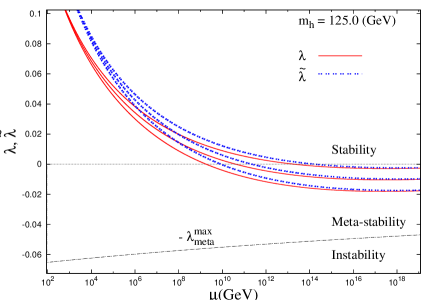
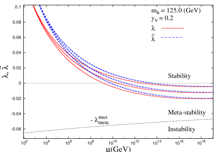
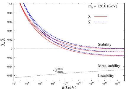
Figure 1: The left panels show the variation of $\lambda$ and $\tilde{\lambda}$ with the renormalization scale for fixed values of the parameters ($m_{h}\,,m_{t}\,,\alpha_{s}$). The upper, middle and lower curves are drawn with the set of parameters ($m_{t},\alpha_{s}$)=$\{(172.3\,\rm{GeV}\,,0.1191)$, $(173.2\,\rm{GeV}\,,0.1184)$, $(174.1\,\rm{GeV}\,,0.1177)\}$ respectively. The right panels show the changes after including the Dirac Yukawa coupling parameter $y_{\nu}$.

In the left panels of Fig. 1, we plot the running of $\tilde{\lambda}$ as a function of the renormalization scale for illustrative values of Higgs mass ($m_{h}$), top mass ($m_{t}$) and strong coupling constant ($\alpha_{s}=g_{3}^{2}/4\pi$). The running of $\lambda$ is also given in the same figure for comparison. The allowed range of values of $m_{t}$ ($173.2\pm 0.9$ GeV) is taken from topmass and that of $\alpha_{s}$ ($0.1184\pm 0.0007$) is taken from alphas . The Higgs mass has been varied between $125-126$ GeV higgsmass .

We have included the corrections to incorporate the mismatch between the top pole mass and $\overline{MS}$ renormalized coupling. This is given as lindner ,

$$y_{t}(m_{t})=\frac{\sqrt{2}m_{t}}{v}(1+\delta_{t}(m_{t}))$$ (32)

$\delta_{t}(m_{t})$ denotes the matching correction at top pole mass. We include the QCD corrections up to three loops qcd while electroweak corrections are taken up to $1$ loop matching ; Schrempp:1996fb . We have also included $\mathcal{O}(\alpha\alpha_{s})$ correction to the matching of top Yukawa and top pole mass Jegerlehner:2003py ; bezrukov . This correction is comparable to QCD correction.

Suitable matching corrections for $\overline{MS}$ renormalized $\lambda$ and the Higgs mass at $\mu=m_{t}$ has been taken up to two loops Sirlin:1985ux ; Degrassi:2012ry . The threshold effect due to the top mass is included. The plots corroborate the fact that for lower values of Higgs mass in the range reported by ATLAS and CMS, the stability of the vacuum till the Planck scale is highly restrictive Degrassi:2012ry . However as demonstrated in the plots, $\tilde{\lambda}\left(M_{pl}\right)$ is not too negative. In this region the potential develops a new minimum from which the transition probability through quantum tunneling is not large enough and consequently the life time of the vacuum remains higher than the age of the universe. This implies that the vacuum is metastable. The tunneling probability (at zero temperature) is given by Isidori:2001bm ; Espinosa:2007qp

$$p=\underset{\mu<\Lambda}{\text{max}}~{}V_{U}\mu^{4}\,\text{exp}\left(-\frac{8\pi^{2}}{3|\lambda(\mu)|}\right),$$ (33)

$\Lambda$ is the cutoff scale. $V_{U}$ is volume of the past light-cone which is taken as $\tau^{4}$ where $\tau$ is the age of the universe. $\tau=4.35\times 10^{17}$ sec Ade:2013ktc . The metastability condition implies $p<1$ which can be translated to a lower bound on $\lambda$ as follows

$$\left|\lambda\right|<\lambda_{\text{meta}}^{\text{max}}=\frac{8\pi^{2}}{3}\frac{1}{4\,\text{ln}\left(\tau\mu\right)}.$$ (34)

This is shown in Fig. 1 as a slanting line dividing the metastability and the instability region.

III.2 Vacuum Stability and Metastability in the Minimal Linear Seesaw Model

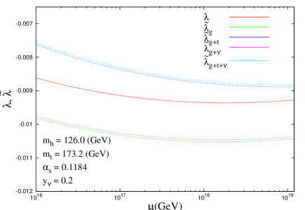
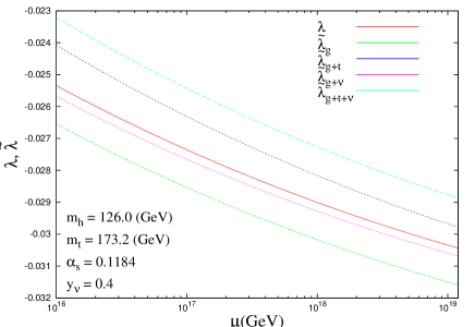
Figure 2: Effect of the contribution from the gauge part, top and neutrinos to the effective coupling $\tilde{\lambda}$

In presence of extra singlets the one loop effective potential of the Higgs field gets an extra contribution from the neutrinos Casas:1999cd . Generalizing the expression in Casas:1999cd for multi-generation case the additional part of the effective potential $V_{\nu}$ can be expressed as,

$${V_{\nu}}\left(\phi_{cl}\right) = -\,\frac{\left(\frac{1}{2}\,\phi_{cl}^{2}\,\left(Y^{{\dagger}}Y\right)_{ii}\right)^{2}}{32\,\pi^{2}}\left[{\rm log}\left(\frac{\frac{1}{2}\,\phi_{cl}^{2}\,\left(Y^{{\dagger}}Y\right)_{ii}}{\mu^{2}}\right)-\frac{3}{2}\right]$$ (35)

$$-\,\frac{\left(\frac{1}{2}\,\phi_{cl}^{2}\,\left(Y\,Y^{{\dagger}}\right)_{jj}\right)^{2}}{32\,\pi^{2}}\left[{\rm log}\left(\frac{\frac{1}{2}\,\phi_{cl}^{2}\,\left(YY^{{\dagger}}\right)_{jj}}{\mu^{2}}\right)-\frac{3}{2}\right]$$

where $\phi_{cl}$ denotes the classical value of the Higgs field. This is obtained in the limit $\phi_{cl}>>$ the mass of the singlet field. $Y$ denotes the $n\times 3$ Yukawa coupling matrix. Note that the above equation is in the diagonal basis for $Y^{\dagger}Y$ and $YY^{\dagger}$. The first contribution in the above expression comes from the light neutrinos ($i=1,2,3$) while the second one comes from the heavy neutrinos ($j=1,...,n$) for $n$ heavy neutrinos. This gives rise to an additional contribution (at 1-loop) towards the effective self coupling $\tilde{\lambda}$

$$\tilde{\lambda}_{\nu} = -\,\frac{1}{32\,\pi^{2}}\left[\left(\left(Y^{{\dagger}}Y\right)_{jj}\right)^{2}\left({\rm ln}\,\frac{\left(Y^{{\dagger}}Y\right)_{jj}}{2}-1\right)+\left(\left(Y\,Y^{{\dagger}}\right)_{jj}\right)^{2}\left({\rm ln}\,\frac{\left(Y\,Y^{{\dagger}}\right)_{jj}}{2}-1\right)\right]$$ (36)

This is to be added to the right hand side of Eq. 31. In our case, $Y=Y_{\nu}^{\prime}=\sqrt{2}m_{D}^{\prime}/v$, $n=2$, $(Y^{{\dagger}}Y)^{dia}\approx Dia(0,0,y_{\nu}^{2})$ and $(YY^{{\dagger}})^{dia}\approx Dia(0,y_{\nu}^{2})$ in the limit of $y_{s}<<y_{\nu}$.

The presence of the singlet fields also modify the SM Renormalization Group Equations (RGEs) for the Yukawa couplings and the Higgs self coupling, for energies higher than the mass of the singlets. Including the corrections due to the neutrino Yukawa couplings up to one loop, the modified $\beta$ function governing the running of $\lambda$ is given as,

$${\beta^{\prime}}_{\lambda}^{(1)} = \beta_{\lambda}^{(1)}+4{\mathrm{Tr}({Y_{\nu}}^{\prime\dagger}Y_{\nu}^{\prime}})\lambda-2{\mathrm{Tr}}[({Y_{\nu}}^{\prime\dagger}Y_{\nu}^{\prime})^{2}],$$ (37)

where $Y_{\nu}^{\prime T}=\left(Y_{\nu}^{T},~{}Y_{S}^{T}\right)$. The one loop $\beta$ functions corresponding to the Yukawa couplings $Y_{u}$, $Y_{d}$ and $Y_{l}$ also acquire additional factors containing ${Y_{\nu}}^{\prime\dagger}Y_{\nu}^{\prime}$ 1-loop-rg . Finally, one needs to include the RG running of the coupling $Y_{\nu}^{\prime}$ which is governed by the following equation:

$$16\pi^{2}\mu\frac{dY_{\nu}^{\prime}}{d\mu}={Y_{\nu}^{\prime}}\left[\frac{3}{2}{Y_{\nu}}^{\prime\dagger}Y_{\nu}^{\prime}-\frac{3}{2}{Y_{l}}^{\dagger}Y_{l}+T-\frac{9}{20}g_{1}^{2}-\frac{9}{4}g_{2}^{2}\right].$$ (38)

In this case the quantity $T$ is defined as,

$$T = {\mathrm{Tr}}\left[3{Y_{u}}^{\dagger}Y_{u}+3{Y_{d}}^{\dagger}Y_{d}+{Y_{l}}^{\dagger}Y_{l}+{Y_{\nu}}^{\prime\dagger}Y_{\nu}^{\prime}\right].$$ (39)

RG equation for neutrino Yukawa coupling is taken up to one loop 1-loop-rg .

The $Y_{\nu}^{\prime}$ dependence of the beta function of $\lambda$ is in terms of Tr$\left[{Y_{\nu}}^{\prime\dagger}Y_{\nu}^{\prime}\right]$ and Tr$\left[({Y_{\nu}}^{\prime\dagger}Y_{\nu}^{\prime})^{2}\right]$ only. From the parameterization of $Y_{\nu}$ and $Y_{S}$, we find

$$\text{Tr}\left[{Y_{\nu}}^{\prime\dagger}Y_{\nu}^{\prime}\right] = y_{\nu}^{2}+y_{s}^{2}\simeq y_{\nu}^{2},$$

$$\text{Tr}\left[{Y_{\nu}}^{\prime\dagger}Y_{\nu}^{\prime}{Y_{\nu}}^{\prime\dagger}Y_{\nu}^{\prime}\right] = y_{\nu}^{4}+2y_{\nu}^{2}y_{s}^{2}\rho^{2}+y_{s}^{4}\simeq y_{\nu}^{4},$$ (40)

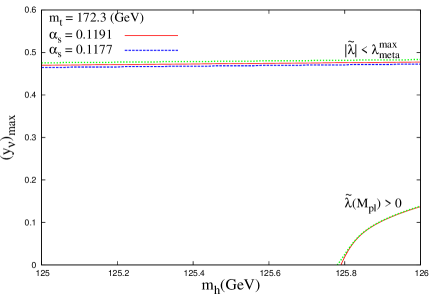
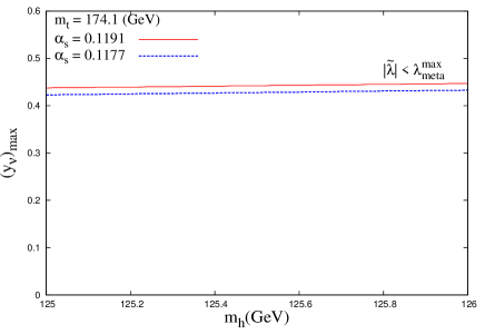
Figure 3: The allowed region of $y_{\nu}$ with varying Higgs mass from the consideration of meta stability $\left(\left|\tilde{\lambda}\right|<\lambda_{\text{meta}}^{\text{max}}\right)$ and absolute stability $\left(\tilde{\lambda}(M_{pl})\geq 0\right)$. The region below the curves is allowed.

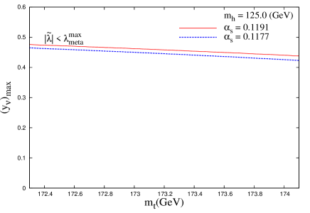
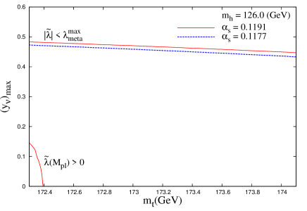
Figure 4: Same as in Fig. 3 with varying top mass.

since $y_{s}<<y_{\nu}$. The exact equalities in the above expressions are also valid even without the parameterization of Eq. (19,22). However $\rho$ remains undetermined. Also, in this case the smallness of $y_{s}$ makes the trace terms to be dependent only on $y_{\nu}$ and hence $\beta_{\lambda}$ depends on only one unknown parameter (i.e.$\,y_{\nu}$). Also we can see from Eq. (40) that the trace terms do not depend on the neutrino oscillation parameters. In addition, under the approximation of $y_{s}<<y_{\nu}$, there is no dependence on mass hierarchy as well (only $\rho$ depends on hierarchy).

In Fig. 1 we show the effect of inclusion of this term on the running of ${\lambda}$. As expected, $\tilde{\lambda}$ becomes more negative near Planck scale in presence of the seesaw term. The figures are obtained including the heavy neutrino contribution to the effective potential.

In Fig. 2 we explicitly display the effect of inclusion of the neutrino contribution in the effective potential. The left panel is for $y_{\nu}=0.2$ and the right panel is for $y_{\nu}=0.4$. The solid-red curve shows the self-coupling $\lambda$. Comparing the two plots for this in the two panels we see that the higher value of $y_{\nu}$ makes $\lambda$ more negative in the right panel. The dashed-green curve shows the evolution of the effective self-coupling due to the contribution of the gauge fields while the small-dashed-blue curve shows the effect of inclusion of the contribution from the top quarks. We see that since in the expression of effective coupling the gauge contribution and top contribution come with opposite signs, these terms drive $\tilde{\lambda}$ in opposite directions. While the gauge-contribution makes the effective $\lambda$ more negative, the top contribution makes it more positive. The dot-dashed-cyan lines show the contributions from the neutrino. This effect goes in the same direction as the top contribution. The effect is found to be very small for $y_{\nu}=0.2$. However for larger values of $y_{\nu}$ the effect can be non-negligible as can be seen from the right panel for $y_{\nu}=0.4$.

In Fig. 3 we give the plot of the allowed region of $y_{\nu}$ as a function of the Higgs mass for fixed values of top mass and the strong coupling constant. The slanting lines are obtained by imposing the condition given in Eq. (34). $y_{\nu}=0$ corresponds to the SM. The first panel is for $m_{t}=172.3$ GeV. For this value of top mass and $\alpha_{s}=0.1191$, only a tiny parameter space is allowed through the stability condition (i.e. $\tilde{\lambda}(M_{pl})\geq 0$). Inclusion of the neutrino contribution to the effective potential, shown by the dashed-green lines, does not have any discernible effect on the stability bound of $\tilde{\lambda}$ for the values of $y_{\nu}$ concerned. However metastability bound changes by $\sim\,1\%$ as is visible from the figure. The solid-red line is the metastability bound with $\lambda$. The dashed-green line is with $\tilde{\lambda}$ including the neutrino effect. All other metastability bounds including the dashed-blue one in this figure are plotted for $\tilde{\lambda}$ including the neutrino effect. Inclusion of heavy neutrino contribution in $\tilde{\lambda}$ changes the bound on $y_{\nu}\leq 0.483$ as opposed to $y_{\nu}\leq 0.477$ obtained without including the neutrino Yukawa term. The $2^{\text{nd}}$ panel corresponds to a higher value of $m_{t}=174.1$ GeV. In this case we obtain the upper bound $y_{\nu}\mathrel{\hbox to0.0pt{\raise 2.20013pt\hbox{$<$}\hss}{\lower 2.20013pt\hbox{$\sim$}}}0.45$ depending on the value of $\alpha_{s}$. This bound is obtained for a Higgs mass of 126 GeV. For lower values of Higgs mass, the allowed $y_{\nu}$ values are correspondingly lower.

Fig. 4 shows the variation of $y_{\nu}$ with $m_{t}$ for fixed values of Higgs mass. Fig. 5 show the variation of $y_{\nu}$ with $\alpha_{s}$. In general, slightly larger allowed regions are obtained for higher values of Higgs mass, lower values of top mass and higher values of $\alpha_{s}$. From the above figures we can have an overall upper bound on the value of $y_{\nu}$ as

$$y_{\nu}\mathrel{\hbox to0.0pt{\raise 2.20013pt\hbox{$<$}\hss}{\lower 2.20013pt\hbox{$\sim$}}}0.48.$$ (41)

The metastability condition is imposed on the value of $\tilde{\lambda}$ by replacing $\lambda$ with $\tilde{\lambda}$ in Eq. (34).

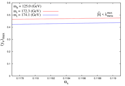
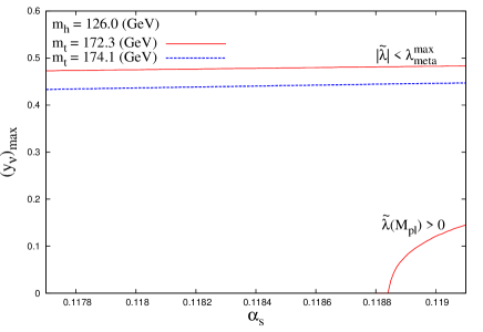
Figure 5: Same as in Fig. 3 with varying strong coupling constant.

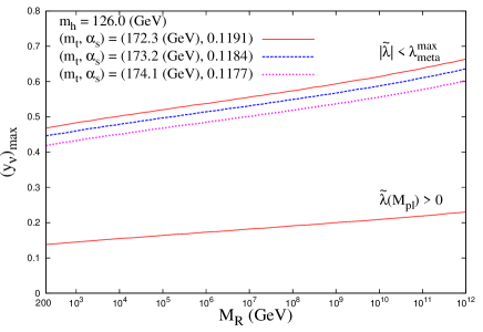
Figure 6: The left-panel shows the upper bound on $y_{\nu}$ as a function of the right-handed neutrino mass from the consideration of metastability $\left(\left|\tilde{\lambda}\right|<\lambda_{\text{meta}}^{\text{max}}\right)$ and absolute stability $\left(\tilde{\lambda}(M_{pl})\geq 0\right)$. For absolute stability there is only one line corresponding to $(m_{t},\alpha_{s})=(172.3\,\text{GeV},0.1191)$ as for other set of parameters no allowed region is available.

The above plots are obtained by keeping $M_{R}$ fixed at 1 TeV. In Fig. 6 we show how the upper bound on $y_{\nu}$ depends on the scale of $M_{R}$.

We see that variation of $M_{R}$ within a few TeV (which is our range of current interest) would not change the bound on $y_{\nu}$ drastically. In fact this trend continues even if $M_{R}$ is increased to higher values. At $M_{R}=10^{12}$ GeV, the upper bound on $y_{\nu}$ obtained is, $y_{\nu}\mathrel{\hbox to0.0pt{\raise 2.20013pt\hbox{$<$}\hss}{\lower 2.20013pt\hbox{$\sim$}}}0.67$. Note that the limits on neutrino mass squared differences from oscillation experiments constraint the product of $y_{\nu}$ and $y_{s}$ as $y_{\nu}y_{s}\approx M_{R}\sqrt{\Delta m^{2}_{atm}}/v^{2}$ for both hierarchies in the limit ${\Delta m_{\odot}^{2}}/{\Delta m^{2}_{atm}}<<1$. Thus, for higher values of $M_{R}$, $y_{s}$ needs to be increased to keep the neutrino mass in the desired range. Beyond $10^{12}$ GeV the contribution from the $y_{s}$ term starts getting significant and hence this needs to be included in the RG evolution.

IV Non-unitarity of Neutrino Mixing Matrix and Lepton Flavor Violation

The mechanism of neutrino oscillation has already indicated that there is flavor violation in the lepton sector. The question arises if there can be flavor violating decays in the charged lepton sector. In typical Seesaw models this rate is very small because of the smallness of the light-heavy mixing. However in TeV scale seesaw models, since lepton number violation (LNV) is separated from the scale of lepton flavor violation (LFV), this may not be the case tevlfv . It is well known that LNV is due to the dimension 5 operator whereas the LFV can be related to the dimension 6 operator. In general, the flavor structure of the coupling strengths of these operators are not correlated. However, in MLSM such a relation can be established from the hypothesis of minimal flavor violation MFV . In this model, the mass and gauge eigenstates are related as,

$$\begin{pmatrix}\nu_{L}&\nu^{c}\end{pmatrix}=U\begin{pmatrix}{\nu_{L}}^{\prime}&{\nu^{c}}^{\prime}\end{pmatrix}$$ (42)

where,

$$\nu^{c}=\begin{pmatrix}N_{R}^{c}&S^{c}\end{pmatrix}.$$ (43)

The leptonic part of the charged current interaction in the gauge basis is given as ,

$$\mathcal{L}_{\rm CC} = \frac{g}{\sqrt{2}}\,\sum_{\alpha=e,\mu,\tau}\overline{\ell}_{\alpha\,L}\,\gamma_{\mu}{\nu}_{\alpha\,L}\,W^{\mu}+\text{h.c.}$$ (44)

This can be expressed in the mass basis as,

$$\mathcal{L}_{\rm CC} = \frac{g}{\sqrt{2}}\,\sum_{\alpha=e,\mu,\tau}\,\sum_{i=1}^{3}\sum_{j=1}^{2}\left[\overline{\ell^{\prime}}_{\alpha\,L}\,\gamma_{\mu}\,U_{l}^{\dagger}\{(U_{L})_{\alpha i}\nu_{Li}^{\prime}+(V)_{\alpha j}N_{Rj}^{c}\}W^{\mu}\right]+\text{h.c.}$$ (45)

The PMNS matrix is defined as

$$U_{\text{PMNS}}=U_{l}^{{\dagger}}\left(1-\frac{1}{2}\epsilon\right)U$$ (46)

where $U_{l}$ is the unitary matrix which takes the left-handed charged lepton fields to their mass basis and other quantities are defined earlier. As we are working in a basis, where charged lepton mass matrix is diagonal, $U_{l}$ is being taken as unity. We note that $U_{PMNS}$ is non-unitary and the correction to unitarity is proportional to $\epsilon/2$.

Table 2: Various experimental constraints from charged lepton flavor violating decays pdg-lfv .

Branching Ratios	Experimental constraints
Br($\mu\rightarrow e\gamma$)	$<5.7\times 10^{-13}$
Br($\tau\rightarrow e\gamma$)	$<3.3\times 10^{-8}$
Br($\tau\rightarrow\mu\gamma$)	$<4.4\times 10^{-8}$
Br($\mu\rightarrow 3e$)	$<1.0\times 10^{-12}$
Br($\tau\rightarrow 3e$)	$<2.7\times 10^{-8}$
Br($\tau\rightarrow 3\mu$)	$<2.1\times 10^{-8}$
Br($\tau\rightarrow e\mu\mu$)	$<1.7\times 10^{-8}$
Br($\tau\rightarrow ee\mu$)	$<1.5\times 10^{-8}$

In this section we consider the branching ratios of LFV decays in MLSM. In view of the recent measurement of $\theta_{13}$ the branching ratios now can be studied in terms of the CP phases. In addition, from the experimental upper limits on LFV processes one can obtain constraints on the parameter $y_{\nu}/M_{R}$ as a function of the CP phases. When combined with the upper bound on $y_{\nu}$ from vacuum (meta)stability as a function of $M_{R}$, the parameter space can be further constrained. Table 2 lists the experimental constraints coming from the charged lepton flavor violating decays pdg-lfv .

Nevertheless, in this section we will concentrate only on the constraints coming from Br($\mu\rightarrow e\gamma$) since this is the most constraining as can be seen from Table 2.

Branching ratio for the process, $\mu\rightarrow e\gamma$ is given by lfv

$$\text{Br}\left(\mu\rightarrow e\gamma\right)=\frac{3\alpha}{8\pi}\left|V_{ei}V_{i\mu}^{{\dagger}}f(x)\right|^{2},$$ (47)

where, $x=\left(\frac{M_{i}^{2}}{m_{W}^{2}}\right)$ and

$$f(x)=\frac{x\left(1-6x+3x^{2}+2x^{3}-6x^{2}\text{ln}x\right)}{2(1-x)^{4}}.$$ (48)

$f(x)$ is a slowly varying function of $x$ ranging from $0$ to $1$ for $x$ between $0$ to infinity. The light-heavy mixing matrix $V$ is defined in Eq. (13). The current experimental constraint on this is mu2egamma   (see, table 2)

$$\text{Br}\left(\mu\rightarrow e\gamma\right)<5.7\times 10^{-13}.$$ (49)

Using the parameterization of $Y_{\nu}$ and $Y_{S}$ in Eq.(19) and (22), we obtain, for normal hierarchy

$$\text{Br}\left(\mu\rightarrow e\gamma\right) = \frac{3\alpha}{8\pi}\frac{y_{\nu}^{4}v^{4}}{4M_{R}^{4}}f^{2}(x)\left(\sqrt{r}\,s_{12}^{2}+2\,r^{(1/4)}\,s_{13}\,s_{12}\,s_{(\alpha+\delta)}+r^{(3/4)}\,c_{23}\,s_{12}\,s2_{12}\,s_{\alpha}/s_{23}\right)s_{23}^{2}$$ (50)

$$+ \mathcal{O}\left(y_{s},(\sqrt{r},s_{13})^{2}\right).$$

In the above expressions and in subsequent part, we have used the following notations

$$s_{ij}=\text{sin}\theta_{ij},\quad c_{ij}=\text{cos}\theta_{ij},\quad s_{\alpha+\delta}=\text{sin}(\alpha+\delta),\quad s_{\delta}=\text{sin}\,\delta,\quad s_{\delta}=\text{sin}\,\delta$$

$$\quad s2_{ij}=\text{sin}2\theta_{ij},\quad c2_{ij}=\text{cos}2\theta_{ij},\quad c_{2\alpha}=\text{cos}2\alpha,\quad s_{2\alpha}=\text{sin}2\alpha\quad\text{etc}.$$ (51)

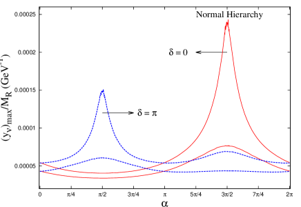
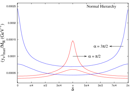
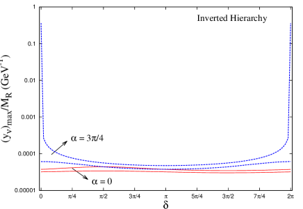
Figure 7: The upper panels show the allowed regions of $y_{\nu}/M_{R}$ vs the CP phases $\alpha$ and $\delta$ for NH while the lower panels are for IH. The area below each curve is consistent with the experimental upper bound on the rate of $\mu\rightarrow e\gamma$. The two lines of the same type (color) correspond to the maximum and minimum value of the upper bound obtained by varying the oscillation parameters over their $3\sigma$ range.

The above equation in conjunction to the upper bound on the $Br(\mu\rightarrow e\gamma)$ can be used to put an upper bound on $y_{\nu}/M_{R}$ as,

$$y_{\nu}/M_{R}<\left[\frac{5.7\times 10^{-11}}{3\alpha v^{4}f^{2}(x)G^{NH}(r,\theta_{ij},\alpha,\delta)}\right]^{1/4}.$$ (52)

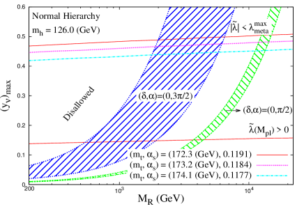
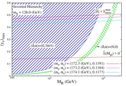
Figure 8: The allowed regions of $y_{\nu}^{max}$ as a function of $M_{R}$ from the combined constraints of $Br(\mu\rightarrow e\gamma)$ and vacuum (meta)stability. The area to the right of the curved lines are allowed from experimental bound on $Br(\mu\rightarrow e\gamma)$ while the area below the slanting lines are allowed from the constraint on vacuum (meta)stability.

Here, the factor $G^{NH}(r,\theta_{ij},\alpha,\delta)$ contains the oscillation parameters. The upper bound on $y_{\nu}/M_{R}$ varies in a range depending on the values of the CP phases. The minimum value of the upper bound occurs at $\alpha+\delta=\frac{\pi}{2}$ while the maximum occurs at $\alpha+\delta=\frac{3\,\pi}{2}$. This is reflected in the top panels in Fig. 7 where we display the allowed values of $y_{\nu}/M_{R}$ as a function of the CP phases. The left most panel displays the variation of the upper bound in $y_{\nu}/M_{R}$ as a function of the Majorana phase $\alpha$. The solid(red) line corresponds to the Dirac phase $\delta=0$ while the dashed (blue) line is for $\delta=\pi$. The other oscillation parameters are marginalized over the 3$\sigma$ range in Table 1 to give the maximum and minimum value of the upper bound on $y_{\nu}/M_{R}$. From the figure it can be inferred that the maximum value of the upper bound on $y_{\nu}/M_{R}$ is

$$y_{\nu}/M_{R}\mathrel{\hbox to0.0pt{\raise 2.20013pt\hbox{$<$}\hss}{\lower 2.20013pt\hbox{$\sim$}}}0.00024(\mathrm{GeV^{-1}}),$$ (53)

which occurs for $\delta=0$ and $\alpha=\frac{3\,\pi}{2}$ for NH.

For IH, the branching ratio can be expressed as,

$$\text{Br}\left(\mu\rightarrow e\gamma\right) = \frac{3\alpha}{8\pi}\frac{y_{\nu}^{4}v^{4}}{4M_{R}^{4}}f^{2}\left(\frac{M_{R}^{2}}{m_{W}^{2}}\right)\frac{1}{4}c_{23}\left(1-s_{2\alpha}s2_{12}\right)\left[c_{23}\left(1+s_{2\alpha}s2_{12}\right)\left(1-s_{13}\right)+2\left(s_{2\alpha}c_{\delta}c2_{12}-c_{2\alpha}s_{\delta}\right)s_{13}s_{23}\right]$$ (54)

$$+\mathcal{O}\left(y_{s},(\sqrt{r},s_{13})^{2}\right).$$

From this one can again get an upper bound on $y_{\nu}/M_{R}$. This is displayed in the lower panels in Fig. 7. As in the case of NH, the value of the upper bound depends on the CP phases. The maximum allowed value in this case is

$$y_{\nu}/M_{R}\mathrel{\hbox to0.0pt{\raise 2.20013pt\hbox{$<$}\hss}{\lower 2.20013pt\hbox{$\sim$}}}0.36(\mathrm{GeV^{-1}}),$$ (55)

which occurs for $\delta=0,\alpha=\frac{3\,\pi}{4}$ as can be seen from the figure. The lines of same line type (color) corresponds to the upper bounds including the uncertainties in the masses and mixing parameters.

The maximum value of $y_{\nu}/M_{R}$ as obtained above can be used to retrieve the maximum value of $y_{\nu}$ for each $M_{R}$. This is shown in Fig. 8. Note that while extracting the bound on $y_{\nu}$ for a particular $M_{R}$ from the figure one has to be careful to ensure that the perturbativity bound on $y_{\nu}$ ($\mathrel{\hbox to0.0pt{\raise 2.20013pt\hbox{$<$}\hss}{\lower 2.20013pt\hbox{$\sim$}}}1$) is not violated. We also superimpose the bounds obtained from consideration of vacuum (meta)stability in this figure. The area to the left of the shaded bands is disallowed from the constraint on the branching ratio $\mu\rightarrow e\gamma$. These bands are obtained for fixed values of the CP phases $(\delta,\alpha)$. The band for each combination of CP phase is obtained by varying the oscillation parameters in their current 3$\sigma$ range. The area below the slanting lines are allowed from the constraint on vacuum (meta)stability. The figure shows that the constraints from Br($\mu\rightarrow e\gamma$) can sometimes further constrain the value of $y_{\nu}$ as obtained from vacuum metastability. For instance, for $M_{R}=200$ GeV and NH, the constraint from Br($\mu\rightarrow e\gamma$) restricts $y_{\nu}$ to be $\leq 0.07$ for values of CP phases $(\delta,\alpha)=\left(0,\frac{3\,\pi}{2}\right)$. For $(\delta,\alpha)=(0,\frac{\pi}{2})$ the maximum allowed value of $y_{\nu}$ is lower. For other combinations of CP phases the bands lie anywhere inside or between the two shaded regions. Thus if we consider all possible values of CP phases then only the region marked disallowed is not compatible with the constraints from Br($\mu\rightarrow e\gamma$) for NH though it was consistent with vacuum metastability constraints. The vacuum stability constraints, on the other hand, are stronger than those obtained from Br($\mu\rightarrow e\gamma$).

For IH and $(\delta,\alpha)=\left(0,\frac{3\,\pi}{4}\right)$, the hatched region extends all the way up to $M_{R}=200$ GeV and there is no significant constraint from $\mu\rightarrow e\gamma$ given the present uncertainty on the neutrino oscillation parameters. Nevertheless for the green hatched region corresponding to $(\delta,\alpha)=(0,0)$, the region to its left is disfavored and $y_{\nu}^{max}$ is constrained to lower values as compared to the bound from vacuum (meta)stability up to a certain value of $M_{R}$. However, if we consider all possible values of CP phases then we can conclude that, given the present uncertainty of oscillation parameters and the CP phases, the vacuum (meta) stability bound on $(y_{\nu})_{max}$ is stronger that that obtained from Br($\mu\rightarrow e\gamma$) for IH.

We note in passing that in this type of models the Higgs boson can decay to two neutrinos of which one is heavy and the other one is a light neutrino, as long as the heavy neutrino is lighter than the Higgs boson. This has been studied in the context of inverse seesaw models and put constraints on the Yukawa coupling $y_{\nu}$ to be $y_{\nu}\mathrel{\hbox to0.0pt{\raise 2.20013pt\hbox{$<$}\hss}{\lower 2.20013pt\hbox{$\sim$}}}$ 0.02 for $M_{R}\mathrel{\hbox to0.0pt{\raise 2.20013pt\hbox{$<$}\hss}{\lower 2.20013pt\hbox{$\sim$}}}$ 120 GeV from the experimental data on the channel $h\rightarrow WW^{*}\rightarrow\ell\ell\nu\nu$ Dev:2012zg ; DeRomeri:2012qd . For larger masses of the heavy neutrino current Higgs searches do not provide any constraint on the parameter space.

On the other hand, the search for heavy singlet neutrinos at LEP by the L3 collaboration in the decay channel $N\rightarrow eW$ showed no evidence of such a singlet neutrino in the mass range between 80 GeV ($\left|V_{\alpha i}\right|^{2}\mathrel{\hbox to0.0pt{\raise 2.20013pt\hbox{$<$}\hss}{\lower 2.20013pt\hbox{$\sim$}}}2\times 10^{-3}$) and 205 GeV ($\left|V_{\alpha i}\right|^{2}\mathrel{\hbox to0.0pt{\raise 2.20013pt\hbox{$<$}\hss}{\lower 2.20013pt\hbox{$\sim$}}}1$) Achard:2001qv . $V_{\alpha i}$ is the mixing parameter between the heavy and light neutrino. Heavy singlet neutrinos in the mass range from 3 GeV up to the Z-boson mass ($m_{Z}$) has also been excluded by LEP experiments from Z-boson decay up to $\left|V_{\alpha i}\right|^{2}\sim 10^{-5}$ Akrawy:1990zq ; Adriani:1992pq ; Abreu:1996pa . In the light of these experimental observations we have chosen the parameter $M_{R}$ to be greater than or equal to 200 GeV in this study.

V 0$\nu\beta\beta$ decay

The half life for neutrino-less double beta decay in presence of heavy singlets is given by 0nunubb ; Chakrabortty:2012mh ,

$$T_{(1/2)}^{-1}={G}\frac{|\mathcal{M}_{\nu}|^{2}}{m_{e}^{2}}\left|U^{2}_{L_{e\,i}}\,m_{i}+<p^{2}>\frac{V^{2}_{e\,i}}{M_{i}}\right|^{2},$$ (56)

where $<p^{2}>$ is given by Tello:2010am

$$<p^{2}>=-m_{e}m_{p}\frac{\mathcal{M}_{N}}{\mathcal{M}_{\nu}}.$$ (57)

$\mathcal{M}_{\nu}$ and $\mathcal{M}_{N}$ denote the nuclear matrix elements corresponding to light and heavy neutrino exchange respectively. The values of the parameters are taken as 0nunubb $G=7.93\times 10^{-15}$ yr^-1, $<p^{2}>=-(182\text{ MeV})^{2}$.

The first term in Eq. (56) is the usual contribution from the left-handed neutrinos. The second term denotes the contribution of the singlet neutrinos. The matrix V is defined in Eq. (13). Taking the most general form of the matrix $m_{D}^{\prime}$ as

$$m_{D}^{\prime}=\begin{pmatrix}m_{d1}&m_{d2}&m_{d3}\\ m_{s1}&m_{s2}&m_{s3}\end{pmatrix},$$ (58)

and $U_{R}$ and $M$ as defined in Eq. (15) and (7) respectively, we obtain,

$$V_{e1}=\frac{i}{\sqrt{2}~{}M_{R}}(m_{s1}^{\ast}-m_{d1}^{\ast}),V_{e2}=\frac{1}{\sqrt{2}~{}M_{R}}(m_{s1}^{\ast}+m_{d1}^{\ast}).$$ (59)

Then the contribution from the heavy part is $2<p^{2}>m_{s1}^{\ast}m_{d1}^{\ast}/M_{R}^{3}\sim 10^{-8}m_{i}$. Thus this contribution is negligible as compared to the contribution from the light sector which is $\sim m_{i}$.

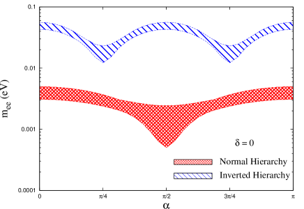
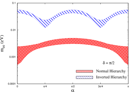
Figure 9: The effective mass governing $0\nu\beta\beta$ as a function of the Majorana phase $\alpha$ for NH (dark (red) shaded curve) and IH (light (blue) shaded curve). The left panel is for $\delta=0$ while the right panel is for $\delta=\pi/2$.

Therefore, $0\nu\beta\beta$ is due to the light neutrinos only and the effective mass is defined as

$$m_{ee}=\left|U^{2}_{L_{e\,i}}\,m_{i}\right|.$$ (60)

Since in this case the lightest mass is zero one can plot the conventional plots of effective mass as a function of the unknown CP phases for both hierarchies.

For NH the effective mass $m_{ee}$ in the limit of the smallest mass $m_{1}\rightarrow 0$ is given as,

$$|m_{ee}|_{NH}=\sqrt{\Delta m^{2}_{atm}}~{}\left|\sqrt{r}s_{12}^{2}c_{13}^{2}e^{2i\alpha}+s_{13}^{2}e^{-2i\delta}\right|.$$ (61)

The maximum is obtained for $(\alpha,\delta)=(0,0)$ or $(\pi/2,\pi/2)$ while the minimum occurs for $(\alpha,\delta)=(0,\pi/2)$ or $(\pi/2,0)$. This is reflected in Fig. 9 by the dark (red) shaded curve which represents the effective mass governing $0\nu\beta\beta$ as a function of the Majorana phase $\alpha$. The shaded portion is due to the 3$\sigma$ uncertainty in the oscillation parameters that appear in the expression of effective mass. The left panel is for $\delta=0$ and the right panel is for $\delta=\pi/2$. The cancellation condition is

$$\sqrt{r}~{}sin^{2}\theta_{12}=\tan^{2}\theta_{13},$$ (62)

which is not satisfied for the current 3$\sigma$ ranges of parameters and therefore the effective mass does not vanish, which is also seen from the figure. For IH the smallest mass is $m_{3}$ which is zero in this model and the effective mass is

$$\left|m_{ee}\right|_{IH}=\sqrt{\Delta m^{2}_{atm}}(c_{12}^{2}c_{13}^{2}e^{-2i\alpha}+s_{12}^{2}c_{13}^{2}e^{2i\alpha}).$$ (63)

For IH the effective mass is independent of the Dirac phase $\delta$. The maximum of $\left|m_{ee}\right|$ occurs for $\alpha=0,\pi/2,\pi$ and the corresponding expression is,

$$\left|m_{ee}\right|_{max}=c_{13}^{2}\sqrt{\Delta m^{2}_{atm}}.$$ (64)

The minimum value is obtained for $\mathrm{\alpha=\pi/4,3\pi/4}$ as,

$$\left|m_{ee}\right|_{min}=c_{13}^{2}cos\,2\theta_{12}\sqrt{\Delta m^{2}_{atm}}.$$ (65)

This is seen from Fig. 9 by the light (blue) shaded curve. $m_{ee}$ for IH is in the range accessible to future neutrinoless double beta decay experiments.

VI Collider Signatures

As mentioned earlier, if the heavy singlet neutrinos have mass less than the Higgs boson mass, then the Higgs boson can have new decay modes Dev:2012zg . For example, the Higgs boson can decay into $h\rightarrow{\bar{\nu}}N$. Now, the singlet neutrinos can decay into $lW$ and $\nu Z$ through the mixing between the heavy neutrinos and the light active neutrinos. At the LHC this will lead to final states such as $pp\rightarrow h\rightarrow\ell^{+}\ell^{-}+E_{T}/\;\>$, where $\ell=e,\mu$. Note that these final states will depend on the Yukawa couplings and one can put bounds on these Yukawa couplings from the existing LHC data on these types of final states Dev:2012zg .

We have considered the singlet neutrino to be heavier than the Higgs boson. In this case one has to look at the 3-body decay modes of the Higgs boson through the virtual heavy neutrino to have similar final states. Obviously, in this case the constraints on the Yukawa couplings will be much less restrictive. In our model we have obtained upper bound on the Yukawa couplings $y_{\nu}$ from the vacuum stability condition and this can be used to test our model at the LHC by looking at the dilepton plus missing $E_{T}$ final states.

One can also have trilepton plus missing $E_{T}$ final states at the LHC from the production of these heavy neutrinos Das:2012ze . For example, at the LHC the heavy neutrinos can be produced through the s-channel $W^{\pm}$ exchange: $u{\bar{d}}\rightarrow\ell^{+}N$ or $u{\bar{d}}\rightarrow\ell^{+}S$. $N$ or $S$ can again decay into $lW$ and $\nu Z$ through $\nu-N$ or $\nu-S$ mixing. This will lead to trilepton plus missing $E_{T}$ final states at the LHC. Now, the trilepton plus $E_{T}/\;\>$ signal is a very clean signal for looking at physics beyond the standard model. In our model, the trilepton final states depend once again on the Yukawa couplings of our model. Using the upper bound on $y_{\nu}$ obtained from vacuum (meta)stability condition, it would be possible to study the present model at the LHC through the trilepton channel. Note that in this model the lepton number violating like-sign di-lepton signal will be suppressed at the colliders because of smallness of $y_{s}$.

VII Conclusion

In this paper we consider the phenomenology of the minimal linear seesaw model consisting of three left-handed neutrinos and two singlet fields. The two singlet fields have opposite lepton numbers. Smallness of neutrino mass is ensured in this model by the tiny lepton number violating coupling ($y_{s}$) of one of the singlets with the left-handed neutrinos. Thus, the masses ($M_{R}$) of the heavy singlet neutrinos can be at the TeV scale even with the Dirac type coupling ($y_{\nu}$) between the other singlet and the heavy state of ${\cal{O}}(1)$. This permits appreciable light-heavy mixing in the model which can have interesting phenomenological consequences. The model predicts one massless neutrino and hence there is only one Majorana phase. The great advantage of this model is that the Yukawa matrices can be fully reconstructed in terms of the oscillation parameters apart from the overall coupling strengths $y_{\nu}$ and $y_{s}$.

The presence of the coupling $y_{\nu}$ in seesaw models tends to destabilize the vacuum further as compared to the SM. This allows one to constrain the coupling strength $y_{\nu}$ from consideration of vacuum (meta)stability. Since the absolute stability of the electroweak vacuum is already severely restricted by the present value of the Higgs mass, this puts a very stringent constraint: $y_{\nu}\mathrel{\hbox to0.0pt{\raise 2.20013pt\hbox{$<$}\hss}{\lower 2.20013pt\hbox{$\sim$}}}0.07$ in a limited region of the parameter space. On the other hand, we show that consideration of the metastability allows one to constrain the coupling strength $y_{\nu}$ as $y_{\nu}\mathrel{\hbox to0.0pt{\raise 2.20013pt\hbox{$<$}\hss}{\lower 2.20013pt\hbox{$\sim$}}}$ 0.48 for $200~{}{\rm GeV}~{}\mathrel{\hbox to0.0pt{\raise 2.20013pt\hbox{$<$}\hss}{\lower 2.20013pt\hbox{$\sim$}}}~{}M_{R}\mathrel{\hbox to0.0pt{\raise 2.20013pt\hbox{$<$}\hss}{\lower 2.20013pt\hbox{$\sim$}}}1~{}{\rm TeV}$. Both these bounds depend on the value of the strong coupling constant ($\alpha_{s}$), the top quark mass ($m_{t}$) and the Higgs boson mass ($m_{h}$). Our analysis includes the effect of neutrino correction to the effective potential at the one loop level.

Bounds on $y_{\nu}/M_{R}$ can be obtained as a function of the CP phases $\alpha$ and $\delta$ from experimental constraints on lepton flavor violating processes. Combined constraints from vacuum (meta)stability and the lepton flavor violating process $\mu\rightarrow e\gamma$ rule out a significant portion of the parameter space in the ($y_{\nu}$–$M_{R}$) plane for NH for masses of $M_{R}\mathrel{\hbox to0.0pt{\raise 2.20013pt\hbox{$<$}\hss}{\lower 2.20013pt\hbox{$\sim$}}}(200-2000)$ GeV depending on the values of the other parameters. On the other hand, contribution of the singlet neutrinos to the neutrinoless double beta decay process is insignificant. The model predicts interesting signatures at the LHC and can be tested using the present and future data. However, a complete collider study merits a separate analysis.

VIII Acknowledgments

The authors wish to thank the sponsors and organizers of the Workshop on High Energy Physics Phenomenology (WHEPP-XI), where the work on this problem started. We want to thank J. Chakrabortty, D. Ghosh, A. Ibarra A. Joshipura, N. Mahajan, S. Mohanty, I. Saha for helpful discussions. S.K. wishes to acknowledge discussions with S. Acharyya, D. Angom, V. Kishore, S. Raut regarding computational analysis. S.K. and S.G wishes to acknowledge the hospitality at the Department of Theoretical Physics, Indian Association for the Cultivation of Science during the course of this work.

References

- (1) S. Chatrchyan et al. [CMS Collaboration], Phys. Lett. B 716, 30 (2012) [arXiv:1207.7235 [hep-ex]].
- (2) G. Aad et al. [ATLAS Collaboration], Phys. Lett. B 716, 1 (2012) [arXiv:1207.7214 [hep-ex]].
- (3) P. A. R. Ade et al. [ Planck Collaboration], arXiv:1303.5076 [astro-ph.CO].
- (4) P. Minkowski, Phys. Lett. B 67, 421 (1977).
- (5) T. Yanagida, in Proceedings of the Workshop on the Unified Theory and the Baryon Number in the Universe (O. Sawada and A. Sugamoto, eds.), KEK, Tsukuba, Japan, 1979, p. 95.
- (6) M. Gell-Mann, P. Ramond, and R. Slansky, Complex spinors and unified theories, in Supergravity (P. van Nieuwenhuizen and D. Z. Freedman, eds.), North Holland, Amsterdam, 1979, p. 315.
- (7) S. L. Glashow, The future of elementary particle physics, in Proceedings of the 1979 Cargèse Summer Institute on Quarks and Leptons (M. Lévy, J.-L. Basdevant, D. Speiser, J. Weyers, R. Gastmans, and M. Jacob, eds.), Plenum Press, New York, 1980, pp. 687–713.
- (8) R. N. Mohapatra and G. Senjanovic, Phys. Rev. Lett. 44 (1980) 912.
- (9) J. Schechter and J. W. F. Valle, Phys. Rev. D 22, 2227 (1980).
- (10) R. Adhikari and A. Raychaudhuri, Phys. Rev. D 84, 033002 (2011) [arXiv:1004.5111 [hep-ph]].
- (11) J. Kersten and A. Y. Smirnov, Phys. Rev. D 76, 073005 (2007) [arXiv:0705.3221 [hep-ph]].
- (12) A. Pilaftsis, Z. Phys. C 55, 275 (1992) [hep-ph/9901206].
- (13) R. N. Mohapatra and J. W. F. Valle, Phys. Rev. D 34, 1642 (1986).
- (14) P. -H. Gu and U. Sarkar, Phys. Lett. B 694, 226 (2010) [arXiv:1007.2323 [hep-ph]].
- (15) H. Zhang and S. Zhou, Phys. Lett. B 685 (2010) 297 [arXiv:0912.2661 [hep-ph]].
- (16) M. Hirsch, S. Morisi and J. W. F. Valle, Phys. Lett. B 679, 454 (2009) [arXiv:0905.3056 [hep-ph]].
- (17) W. -Y. Keung and G. Senjanovic, Phys. Rev. Lett. 50 (1983) 1427.
- (18) P. Bandyopadhyay, E. J. Chun, H. Okada and J. -C. Park, arXiv:1209.4803 [hep-ph].
- (19) P. S. B. Dev, R. Franceschini and R. N. Mohapatra, arXiv:1207.2756 [hep-ph].
- (20) A. Das and N. Okada, arXiv:1207.3734 [hep-ph].
- (21) S. Antusch, M. Blennow, E. Fernandez-Martinez and J. Lopez-Pavon, Phys. Rev. D 80, 033002 (2009) [arXiv:0903.3986 [hep-ph]].
- (22) S. Goswami and T. Ota, Phys. Rev. D 78, 033012 (2008) [arXiv:0802.1434 [hep-ph]].
- (23) E. Fernandez-Martinez, M. B. Gavela, J. Lopez-Pavon and O. Yasuda, arXiv:hep-ph/0703098.
- (24) D. V. Forero, S. Morisi, M. Tortola and J. W. F. Valle, JHEP 1109 (2011) 142 [arXiv:1107.6009 [hep-ph]];
- (25) A. Ilakovac and A. Pilaftsis, Nucl. Phys. B 437, 491 (1995) [hep-ph/9403398].
- (26) S. Antusch, S. Blanchet, M. Blennow and E. Fernandez-Martinez, JHEP 1001, 017 (2010) [arXiv:0910.5957 [hep-ph]].
- (27) W. Rodejohann, Europhys. Lett. 88, 51001 (2009) [arXiv:0903.4590 [hep-ph]].
- (28) J. A. Casas, V. Di Clemente, A. Ibarra and M. Quiros, Phys. Rev. D 62 (2000) 053005 [hep-ph/9904295].
- (29) I. Gogoladze, N. Okada and Q. Shafi, Phys. Lett. B 668 (2008) 121 [arXiv:0805.2129 [hep-ph]].
- (30) F. Bezrukov, M. Y. .Kalmykov, B. A. Kniehl and M. Shaposhnikov, JHEP 1210, 140 (2012) [arXiv:1205.2893 [hep-ph]].
- (31) S. Alekhin, A. Djouadi and S. Moch, Phys. Lett. B 716, 214 (2012) [arXiv:1207.0980 [hep-ph]].
- (32) M. Shaposhnikov and C. Wetterich, Phys. Lett. B 683, 196 (2010) [arXiv:0912.0208 [hep-th]];
- (33) M. Holthausen, K. S. Lim and M. Lindner, JHEP 1202, 037 (2012) [arXiv:1112.2415 [hep-ph]].
- (34) G. Degrassi, S. Di Vita, J. Elias-Miro, J. R. Espinosa, G. F. Giudice, G. Isidori and A. Strumia, JHEP 1208, 098 (2012) [arXiv:1205.6497 [hep-ph]].
- (35) G. Isidori, G. Ridolfi and A. Strumia, Nucl. Phys. B 609, 387 (2001) [hep-ph/0104016].
- (36) J. R. Espinosa, G. F. Giudice and A. Riotto, JCAP 0805, 002 (2008) [arXiv:0710.2484 [hep-ph]].
- (37) J. Ellis, J. R. Espinosa, G. F. Giudice, A. Hoecker and A. Riotto, Phys. Lett. B 679, 369 (2009) [arXiv:0906.0954 [hep-ph]].
- (38) J. Elias-Miro, J. R. Espinosa, G. F. Giudice, G. Isidori, A. Riotto and A. Strumia, Phys. Lett. B 709, 222 (2012) [arXiv:1112.3022 [hep-ph]].
- (39) W. Rodejohann and H. Zhang, JHEP 1206, 022 (2012) [arXiv:1203.3825 [hep-ph]].
- (40) J. Chakrabortty, M. Das and S. Mohanty, arXiv:1207.2027 [hep-ph].
- (41) C. -S. Chen and Y. Tang, JHEP 1204, 019 (2012) [arXiv:1202.5717 [hep-ph]].
- (42) M. B. Gavela, T. Hambye, D. Hernandez and P. Hernandez, JHEP 0909, 038 (2009) [arXiv:0906.1461 [hep-ph]].
- (43) M. Malinsky, T. Ohlsson, Z. z. Xing and H. Zhang, Phys. Lett. B 679, 242 (2009) [arXiv:0905.2889 [hep-ph]].
- (44) L. -J. Hu, S. Dulat and A. Ablat, Eur. Phys. J. C 71, 1772 (2011).
- (45) S. K. Kang and C. S. Kim, Phys. Lett. B 646, 248 (2007). [hep-ph/0607072].
- (46) F. Bazzocchi, Phys. Rev. D 83, 093009 (2011) [arXiv:1011.6299 [hep-ph]].
- (47) P. S. B. Dev and A. Pilaftsis, arXiv:1209.4051 [hep-ph].
- (48) W. Grimus and L. Lavoura, JHEP 0011, 042 (2000) [arXiv:hep-ph/0008179].
- (49) D. V. Forero, M. Tortola and J. W. F. Valle, Phys. Rev. D 86, 073012 (2012) [arXiv:1205.4018 [hep-ph]].
- (50) S. F. King, Phys. Lett. B 439, 350 (1998) [arXiv:hep-ph/9806440].
-
(51)
M. Raidal and A. Strumia,
Predictions of the most minimal seesaw model,
Phys. Lett. B 553, 72 (2003) [hep-ph/0210021]. - (52) R. Barbieri, T. Hambye and A. Romanino, JHEP 0303, 017 (2003) [arXiv:hep-ph/0302118].
- (53) A. Ibarra and G. G. Ross, Phys. Lett. B 591, 285 (2004) [arXiv:hep-ph/0312138].
- (54) M. B. Einhorn and D. R. T. Jones, Phys. Rev. D 46, 5206 (1992).
- (55) M. -x. Luo and Y. Xiao, Phys. Rev. Lett. 90, 011601 (2003) [hep-ph/0207271].
- (56) M. E. Machacek and M. T. Vaughn, Nucl. Phys. B 222, 83 (1983).
- (57) M. E. Machacek and M. T. Vaughn, Nucl. Phys. B 236, 221 (1984).
- (58) M. E. Machacek and M. T. Vaughn, Nucl. Phys. B 249, 70 (1985).
- (59) K. G. Chetyrkin and M. F. Zoller, JHEP 1206 (2012) 033 [arXiv:1205.2892 [hep-ph]].
- (60) L. N. Mihaila, J. Salomon and M. Steinhauser, Phys. Rev. Lett. 108 (2012) 151602 [arXiv:1201.5868 [hep-ph]].
- (61) J. A. Casas, J. R. Espinosa and M. Quiros, Phys. Lett. B 342, 171 (1995) [hep-ph/9409458].
- (62) J. A. Casas, J. R. Espinosa and M. Quiros, Phys. Lett. B 382, 374 (1996) [hep-ph/9603227].
- (63) [Tevatron Electroweak Working Group and CDF and D0 Collaborations], arXiv:1107.5255 [hep-ex].
- (64) S. Bethke, Eur. Phys. J. C 64, 689 (2009) [arXiv:0908.1135 [hep-ph]].
- (65) F. Cerutti, EPS HEP Stockholm, (2013) Slides
- (66) K. Melnikov and T. v. Ritbergen, Phys. Lett. B 482 (2000) 99 [hep-ph/9912391].
- (67) R. Hempfling and B. A. Kniehl, Phys. Rev. D 51 (1995) 1386 [hep-ph/9408313].
- (68) B. Schrempp and M. Wimmer, Prog. Part. Nucl. Phys. 37 (1996) 1 [hep-ph/9606386].
- (69) F. Jegerlehner and M. Y. Kalmykov, Nucl. Phys. B 676, 365 (2004) [hep-ph/0308216].
- (70) A. Sirlin and R. Zucchini, Nucl. Phys. B 266 (1986) 389.
- (71) P. A. R. Ade et al. [Planck Collaboration], arXiv:1303.5062 [astro-ph.CO].
- (72) J. A. Casas, V. Di Clemente, A. Ibarra and M. Quiros, Phys. Rev. D 62, 053005 (2000) [hep-ph/9904295].
- (73) S. Antusch, J. Kersten, M. Lindner and M. Ratz, Phys. Lett. B 538, 87 (2002) [hep-ph/0203233].
- (74) D. N. Dinh, A. Ibarra, E. Molinaro and S. T. Petcov, JHEP 1208 (2012) 125 [arXiv:1205.4671 [hep-ph]]; A. Ibarra, E. Molinaro and S. T. Petcov, Phys. Rev. D 84 (2011) 013005 [arXiv:1103.6217 [hep-ph]].
- (75) V. Cirigliano, B. Grinstein, G. Isidori and M. B. Wise, Nucl. Phys. B 728, 121 (2005) [hep-ph/0507001].
- (76) J. Beringer et al. (Particle Data Group), Phys. Rev. D86, 010001 (2012).
- (77) D. Tommasini, G. Barenboim, J. Bernabeu and C. Jarlskog, Nucl. Phys. B 444, 451 (1995) [hep - ph/9503228].
- (78) J. Adam et al. [MEG Collaboration], Phys. Rev. Lett. 110, 201801 (2013) [arXiv:1303.0754 [hep-ex]].
- (79) V. De Romeri and M. Hirsch, arXiv:1209.3891 [hep-ph].
- (80) P. Achard et al. [L3 Collaboration], Phys. Lett. B 517, 67 (2001) [hep-ex/0107014].
- (81) M. Z. Akrawy et al. [OPAL Collaboration], Phys. Lett. B 247, 448 (1990).
- (82) O. Adriani et al. [L3 Collaboration], Phys. Lett. B 295, 371 (1992).
- (83) P. Abreu et al. [DELPHI Collaboration], Z. Phys. C 74, 57 (1997) [Erratum-ibid. C 75, 580 (1997)].
- (84) M. Mitra, G. Senjanovic and F. Vissani, Nucl. Phys. B 856, 26 (2012) [arXiv:1108.0004 [hep-ph]].
- (85) J. Chakrabortty, H. Z. Devi, S. Goswami and S. Patra, JHEP 1208, 008 (2012) [arXiv:1204.2527 [hep-ph]].
- (86) V. Tello, M. Nemevsek, F. Nesti, G. Senjanovic and F. Vissani, Phys. Rev. Lett. 106 (2011) 151801 [arXiv:1011.3522 [hep-ph]].