Local contractivity of the $\Phi_{0}^{4}$ mapping

Abstract

Previous results about the non trivial solution of the $\Phi^{4}$-equations of motion for the Green’s functions in the Euclidean  space (of $0\leq r\leq 4$ dimensions) in the Wightman Quantum Field theory framework, are reviewed in the $0$ - dimensional case from the following three aspects:

• The structure of the subset $\Phi\subset{\cal B}$ characterized by the signs and “splitting” (factorization properties) is reffined and more explictly described by a subset $\Phi_{0}\subset\Phi$

• The local contractivity of the corresponding $\Phi^{4}_{0}$ mappping is established in a neighborhood of a precise nontrivial sequence $H_{0}\in\Phi_{0}$ using a new norm in the Banach space ${\cal B}$.

• A new $\Phi^{4}_{0}$ iteration is defined in the neighborhood of this sequence $H_{0}\in\Phi_{0}$ and our numerical study displays clearly the stability of $\Phi_{0}$ (the splitting, the bounds and sign properties are perfectly illustrated), and a rapid convergence to the unique fixed point $H^{*}\in\Phi_{0}$(cf. [14]).

1 Introduction

1 A new non perturbative method

Several years ago we started a program for the construction of a non trivial $\Phi^{4}_{4}$ model consistent with the general principles of a Wightman Quantum Field Theory ($Q.F.T.$) [1]. In references [2], [3] we have introduced a non perturbative method for the construction of a non trivial solution of the system of the $\Phi^{4}$ equations of motion for the Green’s functions, in the Euclidean space of zero, one, two and four dimensions.

This method is different in approach from the work done in the Constructive $Q.F.T.$ framework of Glimm-Jaffe and others [4], and the methods of Symanzik who created the basis for a pure Euclidean approach to $Q.F.T.$ [5].

In the $Q.F.T.$ language the interaction of four scalar fields $\Phi(x)$ is described mathematically in the four-dimensional Minkowski space with coordinates:

$$\ x=\{\ \ \vec{x}\in{R}^{3},x_{0}\in{R};||x||=\sqrt{[x_{0}^{2}-\vec{x}^{2}]}\}$$ (1.1)

by the following two-fold set of dynamical equations:

• a nonlinear differential equation (the equation of motion) resulting from the corresponding Lagrangian by application of the variational principle :

  $$-(\vbox{\hrule\hbox{\vrule height=1.0pt,depth=1.0pt\hbox{\kern 1.0pt{${\ }$}\kern 1.0pt}\vrule}\hrule}+m^{2})\Phi(x)=\frac{\Lambda}{\rho+\gamma}[\,:\Phi^{3}(x):-\alpha\Phi(x)\,]$$ (1.2)

• the “conditions of quantization” of the field $\Phi(x)$ expressed by the commutation relations:

  $$[\Phi(x),\Phi(y)]=[\dot{\Phi}(x),\dot{\Phi}(y)]=0$$ (1.3)

  $$[\Phi(x),\dot{\Phi}(y)]=i{\gamma\over\rho+\gamma}\delta^{3}(\vec{x}-\vec{y}),\,x_{0}=y_{0}$$ (1.4)

Here $m>0$ and $\Lambda>0$ are the physical mass and coupling constant of the interaction model, and $\alpha$, $\beta$, $\gamma$, are physically well defined quantities associated to this model, the so called renormalization constants. For the precise definition of the latter and of the normal product $:\Phi^{3}(x):$ we refer the reader to the references [8], [9].

From these equations one can formally derive an equivalent infinite system of non linear integral equations of motion for the Green’s functions (the “vacuum expectation values”) of the theory (analogous, but not identical, to the Dyson -Schwinger equations [10][11]). This dynamical system has been established in $4$ dimensions by using the Renormalized Normal Product of [9].

The method is based on the proof of the existence and uniqueness of the solution of the corresponding infinite system of dynamical equations of motion satisfied by the sequence of the Schwinger functions, i.e. the connected, completely amputated with respect to the free propagator Green’s functions: $H=\{H^{n+1}\}_{n=2k+1,k\in{N}}$, in the Euclidean $r$-dimensional momentum space, ${\cal E}^{rn}_{(q)}$ (where $0\leq r\leq 4$).

Notice that in the previous notations and in what follows ${N}$ means the set of non negative integers and $n$ will always be an odd positive integer.

1.1 The equations of motion for the Schwinger functions and the $\Phi$-Iteration

The infinite system of equations for the Schwinger functions derived by the system 1.1, 1.2, 1.3, 1.4 has precisely the following form in 4 dimensions:

$$H^{2}(q,\Lambda)=-{\Lambda\over{\gamma+\rho}}\{[N^{(3)}_{3}H^{4}]-\Lambda\alpha H^{2}(q,\Lambda)\Delta_{F}(q)\}+{(q^{2}+m^{2})\gamma\over{\gamma+\rho}}$$ (1.5)

and

$$\forall\,n\geq 3,\,(q,\Lambda)\in{\cal E}^{4n}_{(q)}\times{R}$$

$$H^{n+1}(q,\Lambda)={1\over{\gamma+\rho}}\{\,[A^{n+1}+B^{n+1}+C^{n+1}](q,\Lambda)+\Lambda\alpha H^{n+1}(q,\Lambda)\Delta_{F}(q)\}$$ (1.6)

with:

$$A^{n+1}(q,\Lambda)=-\Lambda[N^{(n+2)}_{3}H^{n+3}](q,\Lambda);$$ (1.7)

$$B^{n+1}(q,\Lambda)=-3\Lambda\sum_{\varpi_{n}(J)}[N^{(j_{2})}_{2}H^{j_{2}+2}][N^{(j_{1})}_{1}H^{j_{1}+1}](q,\Lambda);$$ (1.8)

$$C^{n+1}(q,\Lambda)=-6\Lambda\sum_{\varpi_{n}(I)}\prod_{l=1,2,3}[N^{(i_{l})}_{1}H^{i_{l}+1}](q_{i_{l}},\Lambda);$$ (1.9)

Here the notations:

$[N^{(n+2)}_{3}H^{n+3}]$ , $[N^{(j_{2})}_{2}H^{j_{2}+2}][N^{(j_{1})}_{1}H^{j_{1}+1}]$ and $\displaystyle\prod_{l=1,2,3}[N^{(i_{l})}_{1}H^{i_{l}+1}]$, represent the $\Phi^{4}_{4}$ operations which have been introduced in the Renormalized   G-Convolution  Product $(R.G.C.P)$ context of the references [12] [13]. Briefly, the two loop $\Phi^{4}_{4}$ - operation is defined by:

$$[N^{(n+2)}_{3}H^{n+3}]=\int R^{(3)}_{G}[\ H^{n+3}\prod_{i=1,2,3}\Delta_{F}(l_{i})\ ]d^{4}k_{1}d^{4}k_{2}$$ (1.10)

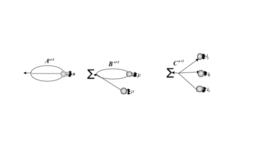
Figure 1: Graphical representation of the global terms of the $\Phi^{4}$ equations of motion

with $R^{(3)}_{G}$ the corresponding renormalization operator for the two loop graph.

The analogous expression for the one loop $\Phi^{4}_{4}$ - operation is the following:

$$[N^{(j_{2})}_{2}H^{j_{2}+2}][N^{(j_{1})}_{1}H^{j_{1}+1}]=H^{j_{1}+1}(q_{j_{1}})\Delta_{F}(q_{j_{1}})\,\int R^{(2)}_{G}[H^{j_{2}+2}\prod_{i=1,2}\Delta_{F}(l_{i})]d^{4}k$$ (1.11)

with $R^{(2)}_{G}$, the corresponding renormalization operator for the two loop graph.

The notation $\Delta_{F}$ indicates the free propagator and the $\Phi^{4}_{4}$ operation $N^{(j_{1})}_{1}$ is exactly the multiplication (“trivial convolution”) by the corresponding free propagator $\displaystyle\Delta_{F}={1\over(\|q\|^{2}+m^{2})}$. Here $\|q\|^{2}$ means the Euclidean norm of the vector $q\in{\cal E}^{4n}_{(q)}$.

The information concerning the special features of the dynamics of four interacting fields, has been obtained through an iteration of these integral equations of motion in the two dimensional case, at fixed coupling constant and at zero external momenta, with the free solution as starting point. This is what was called the “$\Phi$-Iteration” in [2]. The exploration of the detailed structure of the “$\Phi$-Iteration”, has brought forth the particular properties of the different global terms of the equations at every order $\nu$, constructed in terms of the $H^{n+1}_{\nu}$ functions. These properties essentially were:

• (a) alternating signs and splitting (or factorization) properties at zero external momenta:

  $$H^{n+1}(q=0,\Lambda)=-n(n-1)\delta_{n}(\Lambda)H^{n-1}(q=0,\Lambda)[H^{2}(q=0,\Lambda)]^{2}$$ (1.12)

  with $\{\delta_{n}\}$ a bounded increasing sequence of continuous functions of $\Lambda$ and uniformly convergent to some finite positive, $\delta_{\infty}$.

• (b) bounds at zero external momenta and zero momentum dominance bounds, which in turn yield global bounds of the general form:

  $$H^{n+1}(q,\Lambda)\leq n\ !\ \ K^{n}$$ (1.13)

  where $K$ is a finite positive constant independent of $n$.

  These features formed a self-consistent system of conditions conserved by the “$\Phi$-Iteration”. In particular they implied precise “norms” of the sequences of the Green’s functions $H^{n+1}$:

  $$\|H\|=\sup_{q,n,\Lambda}\{M_{n}^{-1}(q,\Lambda)\ \ |H^{n+1}(q,\Lambda)|\}$$ (1.14)

  with the corresponding norm   functions given as follows:

  $\forall\quad(q,\Lambda)\in{\cal E}^{4n}_{(q)}\times{R}^{+*}$

  $$M_{n}(q,\Lambda)=n!\ \ (\ 1/8\ )^{n-5\over 2}(\delta_{\infty})^{n-1\over 2}\ \ \prod_{i=1}^{n}\ \ M_{1}(q_{i},\Lambda),$$ (1.15)

  with:

  $$M_{1}(\ q_{i},\Lambda)=[\|q_{i}\|^{2}+m^{2}]^{1+{1\over 8}}+10\Lambda^{2}$$ (1.16)

  and $\delta_{\infty}$ a universal constant which characterizes the splitting properties presented previously

These norms in turn are conserved and automatically ensure the convergence of the “$\Phi$-Iteration” to the solution. So, the answer to the problem of how to construct the fixed-point method became clear: it would be sufficient first to define a Banach space $\cal B$ using the norms provided by the “$\Phi$-Iteration”. One then should seek a fixed point of the equations of motion inside a characteristic subset $\Phi\subset\cal B$ which exactly imitates the fine structure of the $\Phi$-Iteration.

This is exactly what we tried to realize for $0\leq r\leq 4$ dimensions in the references [2] and [3]. We notice that, even the zero-dimensional corresponding system includes already the supplementary or “renormalization” conditions imposed on the Schwinger functions in order to avoid the infinities appearing in the convolutions of the larger dimensions.

These renormalization constraints constitute the crucial two-fold advantageous aspect of our method. On one hand they provide us with a non trivial solution of the equations of motion even in four dimensions, a basic difference between our approach and the “Constructive  Field   Theory” methods [6][7], which use the generating functional formalism, in order to construct the $Q.F.T.$ Green’s functions-moments of this functional.

On the other hand, this is the essential point that makes our system of equations in zero dimensions equivalent to that obtained directly by derivation of the generating functional (application of the variational principle).

This last point is precisely the argument that we used in reference [13] for the verification of the positivity condition of the zero-dimensional solution.

1.2 The “new mapping”

Using the “$\Phi$-Iteration” which had the free solution as starting point we discovered (in two dimensions, at zero external momenta) at every order $\nu$, the crucial properties presented in the previous section, of the global terms $A^{n+1}$, $B^{n+1}$, $C^{n+1}$, (constructed in terms of the $H^{n+1}_{(\nu)}$ functions), namely: “alternating signs”, “splitting” (or factorization) properties, “bounds at zero external momenta” and “zero momentum dominance bounds”, which in turn yield global bounds and conserved norms.

As we pointed out in the previous section these “conserved norms”(1.1.8) lead to the convergence of the “$\Phi$-Iteration”. So, by introducing an appropriate Banach space ${\cal B}$ defined by these norms and a characteristic subset $\Phi\subset{\cal B}$, which exactly imitates the fine structure of the “$\Phi$-Iteration”, one expects to establish by a fixed point theorem the existence of a non trivial solution inside this subset.

Unfortunately this is not the case. The global terms $A^{n+1}$, $B^{n+1}$, and $C^{n+1}$, (tree terms) (with alternating signs) have the same asymptotic behaviour with respect to $n$. More precisely, at every fixed value of the external momenta,we obtain:

$$A^{n+1}\mathrel{\mathop{\kern 0.0pt\sim}\limits_{n\rightarrow\infty}}(-\ \delta_{\infty})^{n-1\over 2}n!\ n^{2}$$ (1.17)

$$B^{n+1}\mathrel{\mathop{\kern 0.0pt\sim}\limits_{n\rightarrow\infty}}-(-\ \delta_{\infty})^{n-1\over 2}n!\ n^{2}$$ (1.18)

$$C^{n+1}\mathrel{\mathop{\kern 0.0pt\sim}\limits_{n\rightarrow\infty}}(-\ \delta_{\infty})^{n-1\over 2}n!\,n^{2}$$ (1.19)

As far as the behaviour with respect to the external four momenta is concerned they follow the behaviour of the norm functions 1.15, 1.16 (i.e. the corresponding structure of the Banach space).

So despite the convergence of “$\Phi$-Iteration”, (due to the alternating signs of the global terms) the mapping:

$${\cal M}:\,\ {\cal B}\stackrel{{\scriptstyle\cal M}}{{\longrightarrow}}{\cal B}$$ (1.20)

defined by the above equations 1.5, 1.6 is not contractive. As a matter of fact the $n^{2}$ dependence prevents the norms from being conserved.

This is the reason that motivated us to the definition of a new mapping ${\cal M}^{*}$ (given by the following equations which is contractive:

$$H^{n+1^{\prime}}(q,\Lambda)={\delta_{n}^{{}^{\prime}}(q,\Lambda)C^{n+1^{\prime}}(q,\Lambda)\over 3\Lambda n(n-1)};$$ (1.21)

with:

$$\delta_{n}^{{}^{\prime}}(q,\Lambda)=\frac{3\Lambda n(n-1)}{(\gamma+\rho)+D_{n}(H)-\Lambda\alpha\Delta_{F}}$$ (1.22)

and

$$D_{n}(H)={|B^{n+1}|-|A^{n+1}|\over|H^{n+1}|}$$ (1.23)

One can intuitevely understand the contractivity of the new mapping ${\cal M}^{*}$ by looking at the behaviour with respect to $n$ of the function $D_{n}$ (at fixed external momenta). Precisely,

$$D_{n}(H)\mathrel{\mathop{\kern 0.0pt\sim}\limits_{n\rightarrow\infty}}{n^{2}n\ !(\delta_{\infty})^{n-3\over 2}\over n\ !(\delta_{\infty})^{n-1\over 2}}\mathrel{\mathop{\kern 0.0pt\sim}\limits_{n\rightarrow\infty}}{n^{2}\over\delta_{\infty}}.$$ (1.24)

Consequently one has:

$$\delta_{n}^{{}^{\prime}}(q,\Lambda)\mathrel{\mathop{\kern 0.0pt\sim}\limits_{n\rightarrow\infty}}{\delta_{\infty}n(n-1)\over n^{2}}\mathrel{\mathop{\kern 0.0pt\sim}\limits_{n\rightarrow\infty}}\delta_{\infty}$$ (1.25)

By this last argument one can show not only the conservation of the norms (in every dimension $r=0,1,2,3,4$) but also the contractivity of the “new mapping” ${\cal M}^{*}$ to a fixed point inside a characteristic subset $\Phi\subset{\cal B}$, under the following sufficient condition imposed on the renormalized coupling constant:

$$0\leq\Lambda\leq 0.01$$ (1.26)

In an equivalent way, this result means the existence and uniqueness of a non trivial solution (even in four dimensions), of the system. Under the condition 1.26 this solution lies in a neighbourhood of a precise point-sequence of the appropriate subset $\Phi\subset{\cal B}$, the so called fundamental sequence$\{H_{0}\}$.

Consequently, the construction of this non perturbative solution can be realized by iteration of the mapping ${\cal M}^{*}$ inside $\Phi\subset{\cal B}$ starting from the corresponding to every dimension fundamental sequence $\{H_{0}\}$. So, this solution verifies automatically, the“alternating signs” and “splitting” properties, at every value of the external momenta, together with the physical conditions imposed on $H^{2}$ and $H^{4}$-Green’s functions for the definition of the renormalization parameters.

We note that the most important improvement of the method in $4$-dimensions as far as the corresponding properties of the solution are concerned [15] has been precisely the proof of the “alternating signs” and “splitting” properties, at every value of the external momenta, and not only at zero external momenta as we had originally established by the “$\Phi$-Iteration” and the solution of the zero dimensional problem.

The reasons that motivated us for a study in smaller dimensions and not directly in four, were the absence of the difficulties due to the renormalization in two dimensions and the pure combinatorial character of the problem in zero dimensions.

Another useful aspect of the zero dimensional case is the fact that it provides a direct way to test numerically the validity of the method.

1.3 The last “news”:

What are the new developments at zero dimension:

1. The structure of the subset $\Phi\subset{\cal B}$ characterized by the signs, “splitting” (factorization properties) and bounds of the Green’s functions $\left\{H^{n+1}\right\}$ sequences in $\Phi$, is reffined and more explictly described by a new subset $\Phi_{0}\subset\Phi$ in terms of the ”splitting” sequences upper $\left\{\delta_{n_{max}}(\Lambda)\right\}$ and lower $\left\{\delta_{n_{min}}(\Lambda)\right\}$ envelops.

2. The non triviality of the subset $\Phi$ is established in terms of a new basic sequence $\left\{H_{0}\right\}$ that we also use to prove the local contractivity. The stability of $\Phi$ is proved as a consequence of the stability of the subset $\Phi_{0}$ which is directly obtained recurrently thanks to the explicit definitions of the ”splitting” sequences $\left\{\delta_{n_{max}}(\Lambda)\right\}$ and $\left\{\delta_{n_{min}}(\Lambda)\right\}$.

3. The proof of contractivity is simpler in comparison with our previous proofs also due to the fact that we introduce a new norm on the Banach space $\mathcal{B}$.

4. Starting from the fundamental sequence $\left\{H_{0}\right\}$ we define a new $\Phi^{4}_{0}$ iteration and explore numerically in Ref. [14] the behavior of the Green’s functions (essentially the $\delta$ functions), at sufficiently large $n$ and reasonable order of this new iteration.

   The convergence is rapidly established for different values of $\Lambda$ and the sign and splitting properties give consistent results with our theoretical conclusions

2 The existence and uniqueness of the $\Phi^{4}_{0}$ solution

1 The vector space ${\cal B}$ and the $\Phi^{4}_{0}$  equations of motion

Definition 2.1

The space ${\cal B}$.

We introduce the vector space ${\cal B}$ of the sequences $H=\{H^{n+1}\}_{n=2k+1;k\in{N}}$ by the following:

The functions $H^{n+1}(\Lambda)$ belong to the space $C^{\infty}({R}^{+})$ of continuously differentiable numerical functions of the variable $\Lambda\in{R}^{+}$ (which physically represents the coupling constant).

Moreover, there exists a universal (independent of n and of $\Lambda$) positive constant $K_{0}$, such that the following uniform bounds are verified:

$$\forall\ n=2k+1,k\in{N}$$

$$|H^{n+1}(\Lambda)|\leq n\ !(K_{0})^{n}\qquad\forall\,\Lambda\in{R}^{+}$$ (2.27)

Let us now present the zero dimensional analog of the system of equations of motion $(1.2.10...14)$ introduced in the previous chapter.

We suppose that the system of equations under consideration, concerns always the sequences of Euclidean connected and amputated with respect to the free propagators Green’s functions (the Schwinger functions). and that these sequences denoted by $H=\{H^{n+1}\}_{n=2k+1\;,k\in{N}}$ belong to the above space ${\cal B}$.

Taking into account the facts that in the present zero-dimensional case all the external four-momenta are set equal to zero, that the physical mass can be taken equal to $1$ and that the renormalization parameters must be set equal to their trivial values namely:

$$\alpha=0=\rho;\,\,\gamma=1,$$ (2.28)

one directly obtains the corresponding infinite system of equations of motion for the sequence of the Schwinger functions in the following form:

$\forall\ \Lambda\,\in{R}^{+}$

$$H^{2}(\Lambda)=-\Lambda H^{4}(\Lambda)\ \ +1$$ (2.29)

and for all $n\geq 3$,

$$H^{n+1}(\Lambda)=\ \ A^{n+1}(\Lambda)+B^{n+1}(\Lambda)+C^{n+1}(\Lambda)$$ (2.30)

with:

$$A^{n+1}(\Lambda)=\,-\Lambda H^{n+3}(\Lambda);$$ (2.31)

$$B^{n+1}(\Lambda)=\,-3\Lambda\sum_{\varpi_{n}(J)}{n\ !\over j_{1}!j_{2}!}H^{j_{2}+2}(\Lambda)H^{j_{1}+1}(\Lambda);$$ (2.32)

$$C^{n+1}(\Lambda)=\,-6\Lambda\sum_{\varpi_{n}(I)}{n\ !\over i_{1}!i_{2}!i_{3}!\ \sigma_{sym}(I)}\prod_{l=1,2,3}H^{i_{l}+1}(\Lambda)$$ (2.33)

Here the notation $\varpi_{n}(J)$, means the set of different partitions $(j_{1};j_{2})$ of $n$ such that $j_{1}$ is an odd integer and $j_{1}+j_{2}=n$. Respectively $\varpi_{n}(I)$ is the set of triplets of odd numbers-different ordered partitions $(i_{1};i_{2};i_{3})$ of $n$ with $i_{1}\geq i_{2}\geq i_{3}$.

The symmetry-integer $\sigma_{sym}(I)$ is defined by:

$$\sigma_{sym}(I)=\left\{\begin{matrix}\hfill 3!&if&i_{1}=i_{2}=i_{3}\cr\hfill 1&if&i_{1}\neq i_{2}\neq i_{3}\neq i_{1}\cr\hfill&2&otherwise\end{matrix}\right\}$$ (2.34)

2 The subset $\Phi\subset{\cal B}$

2.1 The splitting sequences

Definition 2.2

We first introduce the class ${\cal D}$ of sequences

$$\delta=\{\delta_{n}(\Lambda)\}_{n=2k+1;k\in{N}}\in{\cal B},$$

such that they verify the bounds $(2.1.1)$ in the following simpler form:

$$|\delta_{n}(\Lambda)|\leq\,K_{0},$$ (2.35)

$$\forall\,n=2k+1;\ k\in{N}$$

Definition 2.3

splitting and signs in $\Phi$

A sequence $H\in{\cal B}$ belongs to the subset $\Phi\subset{\cal B}$ if there exists an increasing associated sequence of positive and bounded functions on ${R}^{+}$,

$$\delta=\{\delta_{n}(\Lambda)\}_{n=2k+1;k\in{N}}\in{\cal D},$$

such that the following “splitting” (or factorization) and sign properties are verified:

$$\forall\Lambda\in{R}^{+}$$

$\Phi.1$

$$H^{2}(\Lambda)=1+\Lambda\delta_{1}(\Lambda)\,\hbox{ with:}\,\,\mathrel{\mathop{\kern 0.0pt\lim}\limits_{\Lambda\rightarrow 0}}\delta_{1}(\Lambda)=0$$ (2.36)

$\Phi.2$

$$H^{4}(\Lambda)=-\delta_{3}(\Lambda)[H^{2}(\Lambda)]^{3},\,\hbox{ with:}\,\,\delta_{3}(\Lambda)\leq 6\Lambda,\ \mathrel{\mathop{\kern 0.0pt\lim}\limits_{\Lambda\rightarrow 0}}{\delta_{3}(\Lambda)\over\Lambda}=6$$ (2.37)

$\Phi.3$

$$\forall n\geq 5\qquad H^{n+1}(\Lambda)={\displaystyle\delta_{n}(\Lambda)C^{n+1}\over\displaystyle 3\Lambda n(n-1)},\ \hbox{ with :}\,\ \mathrel{\mathop{\kern 0.0pt\lim}\limits_{\Lambda\rightarrow 0}}{\displaystyle\delta_{n}(\Lambda)\over\displaystyle\Lambda}=3n(n-1)$$ (2.38)

$\Phi.4$

$\forall\,\,n=2k+1$  with  $k\in{N},\,\exists$ positive, (increasing with respect to $n$), continuous functions of $\Lambda$,

$$\delta_{n,max}(\Lambda),\ \delta_{n,min}(\Lambda),$$

uniform limit and bound at infinity independent on $\Lambda$: $\hat{\delta}_{\infty}$, such that:

$$\delta_{n,min}(\Lambda)<\ \delta_{n,max}(\Lambda)$$ (2.39)

$$\delta_{n,min}(\Lambda)\leq\delta_{n}(\Lambda)\leq\delta_{n,max}(\Lambda)$$ (2.40)

$$\mathrel{\mathop{\kern 0.0pt\lim}\limits_{n\rightarrow\infty}}\delta_{n,max}\leq\hat{\delta}_{\infty}$$ (2.41)

Remark 2.1

a.

We first remark that the above “splitting” or factorization properties $\Phi.1,2,3$ are general formulae which simply define the function $\delta_{n}(\Lambda)$ in terms of the Green’s function $H^{n+1}$ and the “tree” function $C^{n+1}$. In other words, for every sequence $H\subset{\cal B}$ the corresponding splitting formulae can be formally written. The particular character of the subset $\Phi$ comes from the fact that the sequence of positive continuous functions $\delta=\{\delta_{n}(\Lambda)\}_{n=2k+1;k\in{N}}\in{\cal B}$ belongs to the class ${\cal D}$ of uniformly bounded functions in ${\cal B}$ and verifies the limit and asymptotic properties $(\Phi.1,2,3,4)$

b.

The sequences $\{\delta_{n,max}(\Lambda)\}_{n=2k+1;k\in{N}}$ and $\{\delta_{n,min}(\Lambda)\}_{n=2k+1;k\in{N}}$ are not uniquely defined. One can choose many such sequences, and of course all of them yield an analogous structure of the subset $\Phi$. Nevertheless, we specify below such a couple of sequences (cf. definition 2.8) for the following reasons:

• a) We shall use these specific splitting sequences: $\{\delta_{n,max}(\Lambda)\}_{n}$ and $\{\delta_{n,min}(\Lambda)\}_{n}$ in order to construct the sequences:

  $$\{H^{n+1}_{max}\}_{n=2k+1;k\in{N}}\in\ {\cal B}\ \ \,\hbox{and}\,\ \{H^{n+1}_{min}\}_{n=2k+1;k\in{N}}\,\in{\cal B}$$

  and the “fundamental sequence” $\{H_{0}\}\in{\cal B}$ (cf. definitions 2.5 and 2.6 below). These sequences define an appropriate neighborhood, the subset $\Phi_{0}\subset\Phi$.

• b) We then show the stability of this subset under the mapping ${\cal M}^{*}$ and the local contractivity of ${\cal M}^{*}$ inside a ball centered at $\{H_{0}\}$.

• c) A new $\Phi^{4}_{0}$ iteration is defined, with starting point the sequence $\{H_{0}\}$ and in the reference [14], we “constructed numerically” the solution of the dynamical system of equs. of the $\Phi^{4}_{0}$ model.

2.2 The “neighborhood” $\Phi_{0}\subset\Phi$

Definition 2.4

$$\delta_{3,max}(\Lambda)=6\Lambda;\qquad\delta_{3,min}(\Lambda)={6\Lambda\over 1+9\Lambda}$$ (2.42)

and  $\forall\,\,n\geq 5$

$$\delta_{n,max}(\Lambda)\,={3\Lambda\ n(n-1)\over 1+3\Lambda\ n(n-1)d_{0}}$$ (2.43)

where $d_{0}=0.01$

$$\delta_{n,min}(\Lambda)\,={3\Lambda\ n(n-1)\over 1+3\Lambda\ n\ (n-1)}$$ (2.44)

Definition 2.5

We first define:

$$H^{2}_{max}(\Lambda)=(1+6\Lambda^{2})^{2};\ \qquad H^{2}_{min}=1$$ (2.45)

$$H^{4}_{max}(\Lambda)=-6\Lambda[1+6\Lambda^{2}]^{6};\ \ H^{4}_{min}(\Lambda)=-{6\Lambda\over 1+9\Lambda}$$ (2.46)

Then, we define recurrently the following sequences, for every $n=2k+1$ with $k\in{N},\ k\geq 2$, by using $\{\delta_{n,max}\}$  and  $\{\delta_{n,min}\}$ introduced above:

(i.)

$$H^{n+1}_{max}={\delta_{n,max}(\Lambda)C^{n+1}_{max}\over 3\Lambda\ n(n-1)}$$ (2.47)

$$H^{n+1}_{min}(\Lambda)={\delta_{n,min}(\Lambda)C^{n+1}_{min}\over 3\Lambda\ n(n-1)}$$ (2.48)

Here $C^{n+1}_{max},C^{n+1}_{min}$, the so called “tree terms”, are defined by analogy to the definition 2.33 of the introduction, precisely:

$$C^{n+1}_{max}=\,-6\Lambda\sum_{\varpi_{n}(I)}{n\ !\over i_{1}!i_{2}!i_{3}!\ \sigma_{sym}(I)}\prod_{l=1,2,3}H^{i_{l}+1}_{max}$$ (2.49)

$$C^{n+1}_{min}=\,-6\Lambda\sum_{\varpi_{n}(I)}{n\ !\over i_{1}!i_{2}!i_{3}!\ \sigma_{sym}(I)}\prod_{l=1,2,3}H^{i_{l}+1}_{min}$$ (2.50)

(ii.) In an analogous way we define:

$$A^{n+1}_{max}=\,-\Lambda H^{n+3}_{max};\qquad A^{n+1}_{min}=\,-\Lambda H^{n+3}_{min}.$$ (2.51)

(iii.)

$$B^{n+1}_{max}(\Lambda)=\,-3\Lambda\sum_{\varpi_{n}(J)}{n\ !\over j_{1}!j_{2}!}H^{j_{2}+2}_{max}H^{j_{1}+1}_{max};$$ (2.52)

$$B^{n+1}_{min}(\Lambda)=\,-3\Lambda\sum_{\varpi_{n}(J)}{n\ !\over j_{1}!j_{2}!}H^{j_{2}+2}_{min}H^{j_{1}+1}_{min}.$$ (2.53)

Now, we introduce the “fundamental sequence”.

Definition 2.6

$$H^{2}_{0}(\Lambda)=1-\Lambda H^{4}_{min}\ \ \$$ (2.54)

$$H^{4}_{0}(\Lambda)=-\delta_{3,0}(\Lambda)[H^{2}_{0}]^{3}\quad\hbox{with}\quad\delta_{3,0}(\Lambda)=\displaystyle{\frac{6\Lambda}{1+9\Lambda H^{2}_{min}-\displaystyle{\frac{\Lambda|H^{6}_{min}|}{|H^{4}_{max}|}}}}$$ (2.55)

and for every $n\geq 5$

$$H^{n+1}_{0}(\Lambda)={\delta_{n,0}(\Lambda)C^{n+1}_{0}(\Lambda)\over 3\Lambda n(n-1)};$$ (2.56)

with:

$$C^{n+1}_{0}(\Lambda)=-6\Lambda\sum_{\varpi_{n}(I)}{n\ !\over i_{1}!i_{2}!i_{3}!\ \sigma_{sym}(I)}\prod_{l=1,2,3}H^{i_{l}+1}_{0}(\Lambda);$$ (2.57)

$$\delta_{n,0}(\Lambda)=\frac{3\Lambda n(n-1)}{1+D_{(n,min)}(H)}$$ (2.58)

and

$$D_{(n,min)}(H)=\displaystyle{\frac{|B^{n+1}_{min}|}{|H^{n+1}_{min}|}-\frac{|A^{n+1}_{max}|}{|H^{n+1}_{max}|}}$$ (2.59)

Here the terms $B^{n+1}_{min}$ and $A^{n+1}_{max}$ are defined by the definitions 2.53 and 2.51 respectively.

Definition 2.7

The subset $\Phi_{0}$

Taking into account the sequences of definitions 2.8 and 2.5 we introduce the following subset $\Phi_{0}\subset\Phi$:

$$\Phi_{0}=\left\{H\in\Phi:|H^{n+1}_{min}|\ \leq|H^{n+1}|\leq|H^{n+1}_{max}|,\quad\forall n=2k+1,\ k\in\ {N}\right\}$$ (2.60)

Proposition 2.1

(the non triviality of $\Phi_{0}$ and $\Phi$)

The set of sequences $\Phi_{0}$ given by the definition 2.7 is a nontrivial subset of the space ${\cal B}$.

Proof of Proposition 2.1

From the previous definitions of the sequences $\{\delta_{n,max}\}\,\ \ \{\delta_{n,min}\}$ (cf. definition  2.8) and of the sequences $\{H^{n+1}_{max}\},\,\ \{H^{n+1}_{min}\}$, $\{H_{0}\}$ (cf. definitions 2.5 and 2.6), and the obvious strict inequality

$$\delta_{n,max}(\Lambda)>\ \delta_{n,min}(\Lambda)\ \ \forall\ n=2k+1;k\in{N}^{*}$$

one directly ensures that:

• a) The previously defined fundamental sequence $H_{0}$ satisfies the properties $(\Phi.1,2,3,4)$ of definition 2.3 and definition 2.7 for every $\Lambda$ in the interval $]0;0.05]$

• b) The set $\Phi_{0}$ is a non trivial subset of the set $\Phi$, which in turn is a non trivial subset of ${\cal B}$.  $\blacksquare$

Let us now present some definitions and auxiliary results, that one could easily obtain from the previous definitions.

Proposition 2.2

$\forall n\geq 5$ the tree terms $C^{n+1}_{min}$ and $C^{n+1}_{max}$ verify:

$$\begin{array}[]{l}|C^{n+1}_{min}|\geq\ |\bar{C}^{n+1}_{min}|\\ \\ |C^{n+1}_{max}|\leq\ |\bar{C}^{n+1}_{max}|\end{array}$$

where:

$$\begin{array}[]{l}|\bar{C}^{n+1}_{min}|=\mathcal{T}_{n}|C^{n+1}_{(n/3,n/3,n/3)(min)}|\\ \\ |\bar{C}^{n+1}_{max}|=\mathcal{T}_{n}|C^{n+1}_{(n-2,1,1)(max)}|\end{array}$$ (2.61)

Where we have to take into account the result of ref. [2, c] about the number $\mathcal{T}_{n}$ of different partitions of the set $\varpi_{n}(I)$ in the sum $\sum\limits_{\varpi_{n}(I)}$ precisely:
for every $n\geq 9$ :

$$\mathcal{T}_{n}=\frac{(n-3)^{2}}{48}+\frac{(n-3)}{3}+1$$ (2.62)

2.3 The “sweeping factors”

Definition 2.8

For every $H\in\Phi_{0}$, we introduce the sequence of functions,

$$\{Y_{n}(H)\}_{n=2k+1;k\in{N}^{*}}\in{\cal D}\subset{\cal B}$$

called the “sweeping factors” and defined as follows:

$$Y_{3}=\frac{1}{6};\quad Y_{5}=\frac{1}{20}$$ (2.63)

and for every $n\geq 7$

$$Y_{n}(H)=\frac{-C^{n+1}}{3\Lambda n^{2}(n-1)^{2}H^{n-1}[H^{2}]^{2}}$$ (2.64)

The limits at $\Lambda\rightarrow\ 0$ and positivity of the coupling constant and that of the splitting sequences implies directly (in view of the previous definitions) the limits, the “good sign” properties $(-1)^{\frac{(n-1)}{2}}$ of the Schwinger functions, the complete “splitting” (or factorization) properties, together with the combinatorial asymptotic behaviour of the $H^{n+1}$ functions. We present these results without proof by the following statement.

2.4 “Alternating signs” and “complete ‘splitting‘”

Proposition 2.3

Let $H\in\,\Phi_{0}$, then for every $\Lambda\in]0;0.035]$

• $$\lim_{\Lambda\rightarrow 0}H^{2}(\Lambda)=1,\qquad\lim_{\Lambda\rightarrow 0}\frac{H^{4}(\Lambda)}{\Lambda}=-6$$ (2.65)

  and

  $$\forall\,n\geq 5,\quad\lim_{\Lambda\rightarrow 0}\frac{H^{n+1}(\Lambda)}{(-\Lambda)^{(n-1)/2}}=n!c_{n}$$ (2.66)

  where the positive constants $c_{n}$ are recurrently defined by:

  $$c_{n}=6\sum_{\varpi_{n}(I)}\frac{\prod_{j=1,2,3}c_{i_{j}}}{\sigma_{sym}(I)}\qquad\hbox{with}\quad c_{3}=1=c_{1}.$$ (2.67)

• for every $n\geq 3$ we have:

  a)

  $$H^{n+1}(\Lambda)=-n(n-1)\delta_{n}(\Lambda)\,Y_{n}(H)H^{n-1}[H^{2}]^{2}$$ (2.68)

  b)

  $$H^{n+1}(\Lambda)=n!(-1)^{\frac{(n-1)}{2}}\,\displaystyle{[H^{2}]^{n}}\prod_{m=3}^{n}Y_{m}(H)\delta_{m}(\Lambda)$$ (2.69)

3 The new mapping ${\cal M^{*}}$ and the stability of $\Phi_{0}$

We now define the new mapping ${\cal M^{*}}$ and then prove the stability of the subset $\Phi_{0}$ (and consequently of $\Phi$) under the action of this mapping.

Definition 3.1

The new mapping ${\cal M^{*}}$ .

Let $H\in\ \Phi_{0}$ We define the following application ${\cal M^{*}}:\,\Phi_{0}\stackrel{{\scriptstyle\cal M^{*}}}{{\longrightarrow}}{\cal B}$ by:

$$H^{2^{\prime}}(\Lambda)=1-\Lambda H^{4}(\Lambda)$$ (3.70)

$$H^{4^{\prime}}(\Lambda)=-\delta_{3}^{\prime}(\Lambda)[H^{2^{\prime}}]^{3}\quad\hbox{with}\quad\delta_{3}^{{}^{\prime}}(\Lambda)=\frac{6\Lambda}{1+\ D_{3}}$$ (3.71)

$$\mbox{and}\quad D_{3}=6\Lambda H^{2}\left(3/2-\frac{|H^{6}|}{6|H^{4}||H^{2}|}\right).$$ (3.72)

Moreover:

$$\forall\ n\geq 5\qquad H^{n+1^{\prime}}(\Lambda)=\displaystyle{\delta_{n}^{{}^{\prime}}(\Lambda)C^{n+1^{\prime}}\over\displaystyle 3\Lambda n(n-1)}$$ (3.73)

Here:

$$\delta_{n}^{{}^{\prime}}(\Lambda)=\frac{3\Lambda n(n-1)}{1+D_{n}(H)}$$ (3.74)

with:

$$D_{n}(H)={|B^{n+1}|-|A^{n+1}|\over|H^{n+1}|}$$ (3.75)

Remark 3.1

Notice that in the above definition the functional $D_{n}(H)$ is obtained in terms of the absolute values of the Green’s functions, thanks to the hypothesis $H\in\Phi_{0}\subset\ \Phi$ which implies the good sign properties of the Green’s functions.

Taking into account the infinite system of equations of motion of the Green’s functions (cf. 2.1.3…7), the structure of the subset $\Phi$ (cf.def.2.3) and the above definition 3.1, one easily verifies the equivalence of the mappings ${\cal M}$ and ${\cal M^{*}}$.

Theorem 3.1

The stability of the subset $\Phi_{0}\subset{\Phi}$

Let $H\in\Phi_{0}$ then:

$${\cal M^{*}}(H)\subset\Phi_{0}$$

under the condition:

$$0<\Lambda\leq 0.05$$

The proof of the stability of $\Phi_{0}$ under the mapping ${\cal M^{*}}$ is given in Appendix I of section 5 by using the following four auxiliary propositions also established in this Appendix.

Proposition 3.1

Signs and bounds for $n=1,\ 3,\ 5$

Let ${H\in\Phi_{0}}$ then   $\forall\Lambda\leq 0.05$:

• $$H^{2^{\prime}}>0;\ \quad H^{4^{\prime}}<0,\quad H^{6^{\prime}}>0.$$ (3.76)

• $$\begin{array}[]{l}H^{2}_{min}<H^{2^{\prime}}<H^{2}_{max}\\ \\ |H^{4}_{min}|<\ |H^{4^{\prime}}|<|H^{4}_{max}|\\ \\ H^{6}_{min}<H^{6^{\prime}}<H^{6}_{max}\end{array}$$ (3.77)

Proposition 3.2

Let ${H\in\Phi_{0}}$ then   $\forall\Lambda\leq 0.05$:

The functional $A^{n+1}(H)$ given by definition 2.1 verifies the following properties:

• the “good sign” property:

  $$\forall\ n=2k+1\ (k\geq 1)\ \ A^{n+1}=(-1)^{\frac{n-1}{2}}|A^{n+1}|$$

• $\forall\ n=2k+1\ (k\geq 3)$, the sequence:

  $${\frac{|A^{n+1}_{max}|}{n(n-1|H^{n+1}_{max}|}}$$

  decreases with increasing $n$.

Proposition 3.3

Let ${H\in\Phi_{0}}$ then   $\forall\Lambda\leq 0.05$:

The functional $B^{n+1}(H)$ given by definition 2.1 verifies the following properties:

• the “opposite sign” property:

  $$\forall\ n=2k+1,\ (k\geq 1)\ \ B^{n+1}=(-1)^{\frac{n-3}{2}}|B^{n+1}|$$

• $\forall\ n=2k+1\ (k\geq 3)$, the sequence:

  $${\frac{|B^{n+1}_{min}|}{n(n-1)|H^{n+1}_{min}|}}$$

  increases with increasing $n$.

Proposition 3.4

Let ${H\in\Phi_{0}}$ then   :

$\forall n\geq 7$

i)

$${\lim_{\Lambda\rightarrow 0}D_{n}(\Lambda)}=0$$

ii) $\forall\Lambda\leq 0.05$ the sequence:

$${\frac{D_{(n,min)}(H)}{3\Lambda n(n-1)}}$$

increases with increasing $n$.

iii) There exists a finite positive real number $1>d_{n}>\ d_{0}$  such that:

$${\frac{1}{2}\geq\frac{D_{n}(H)}{3\Lambda n(n-1)}}\geq d_{n}\quad\mbox{and}\ \ \displaystyle{\lim_{n\to\infty}d_{n}=d_{0}=\frac{1}{\delta_{\infty}}}$$

Reminder:

$$D_{n}(H)={|B^{n+1}|-|A^{n+1}|\over|H^{n+1}|}$$ (3.78)

4 Construction of the $\Phi^{4}_{0}$  unique and non trivial solution

1 The Banach space

In this third part of the study of the $\Phi^{4}_{0}$ problem we present the construction of the unique non trivial solution inside the subset $\Phi$, by the following three steps:

i.

We introduce a precise norm ${\cal N}$ inside ${\cal B}$ and show the closedeness and completeness of $\Phi_{0}$ in the induced norm.

ii.

We prove the contractivity of ${\cal M}^{*}$ inside a neighborhood $\Phi_{0}$ and consequently the existence and uniqueness of a fixed point of the initial mapping ${\cal M}$ inside this particular subset of ${\cal B}$.

iii.

For the construction of the solution we realized (cf.[14]) an iteration of the mapping ${\cal M}^{*}$, starting from the particular sequences $\{\delta_{n(max)}\}$ and $\{\delta_{n(min)}\}$, which define the neighborhood of the “fundamental sequence” $H_{0}$ introduced in the previous section.

Definition 4.1

We introduce the following mapping ${\cal N}$ from ${\cal B}$ to ${R}^{+}$:

$$\begin{array}[]{l}{\cal N}:\ {\cal B}\rightarrow{R}^{+}\\ \ \ \ \ H\mapsto\|H\|\ \ \hbox{with:}\ \ \|H\|=\displaystyle{\sup_{\Lambda;n}}\displaystyle{\frac{|H^{n+1}|}{M_{n}}}\end{array}$$ (4.79)

Here $\forall\ \ \Lambda\in{R}^{+}$:

$$M_{1}(\Lambda)=H^{2}_{max}=(1+6\Lambda^{2})^{2};\quad M_{3}(\Lambda)=\,\delta_{3,max}(M_{1})^{3};\ \$$ (4.80)

and for every $n\geq 5$

$$\begin{array}[]{l}M_{n}(\Lambda)=\ n(n-1)\delta_{n,max}M_{n-2}(M_{1})^{2}\\ \\ \end{array}$$ (4.81)

Remark 4.1

1. We note that the above function ${\cal N}$ defines a finite norm inside a non empty subspace ${\cal B}_{c}$ of ${\cal B}$. This subspace ${\cal B}_{c}$ evidently contains $\Phi$ (and $\Phi_{0}$) and it is a Banach space with respect to the ${\cal N}$- topology.

2. Using the above definition 4.81 of the norm in ${\cal B}$, we introduce a ball-neighborhood $S_{\rho}(H_{0})\subset\Phi_{0}$ of the fundamental sequence and show by theorem 4.1 which follows, the local contractivity of ${\cal M}^{*}$ inside it.

2 The local contractivity

Definition 4.2

$$\begin{array}[]{l}S_{\rho}=\{H\in\Phi_{0}:\|H-H_{0}\|\leq\rho\}\\ \\ \mbox{with}\ \ \rho=\displaystyle{\sup_{n}\frac{\{\ \delta_{n,max}-\delta_{n,min}\}}{\delta_{n,max}}}\end{array}$$ (4.82)

In view of the definition 2.8 of the sequences $\{\ \delta_{n,max}\}\ \ \mbox{and}\ \ \ \{\delta_{n,min}\}$, we directly verify the following:

Proposition 4.1

$$\rho=\displaystyle{\lim_{n\to\infty}\frac{\{\ \delta_{n,max}-\delta_{n,min}\}}{\delta_{n,max}}}=1-d_{0}$$ (4.83)

In Appendix II we give in detail the proof of the following:

Theorem 4.1

The local contractivity of the mapping ${\cal M}^{*}$  in $S_{\rho}(H_{0})\ \subset\Phi_{0}$

i.

The subset (ball) $S_{\rho}(H_{0})\ \subset\Phi_{0}$ is a complete metric subspace of ${\cal B}_{c}$ in the induced topology.

ii.

There exists a finite positive constant $\Lambda^{*}(\approx 0.45)$ such that the mapping ${\cal M}^{*}$ is locally contractive inside $S_{\rho}(H_{0})\ \subset\Phi_{0}$.

iii.

When $\Lambda\in]0,\Lambda^{*}]$ the unique non trivial solution of the $\Phi_{0}^{4}$ equations of motion lies in the neihbourhood $S_{\rho}(H_{0})\ \subset\Phi_{0}$ of the fundamental sequence $H_{0}$.

Acknowledgments

The author is grateful to J.Bros for his constant encouragement during the various phases of this work and for a critical reading of the manuscript.

5 APPENDIX I

1 Proof of propositions 3.1, 3.2, 3.3, 3.4

1. Proof of proposition 3.1

   • n=1

     $$\begin{array}[]{l}\mbox{From \ref{def.2.5}, \ref{def.3.1} and the hypothesis we have}:\\ H^{2^{\prime}}=1-\Lambda H^{4},\ H^{4}=(-1)|H^{4}|\ \ \mbox{and}\ \ |H^{4}|\leq|H^{4}_{max}|\\ \\ \Rightarrow\ \ H^{2^{\prime}}>0\ \ \mbox{and}\ \ \ |H^{2^{\prime}}|\leq 1+6\Lambda^{2}(1+6\Lambda^{2})^{6}).\\ \mbox{Then we verify that for every}\Lambda\leq 0.05\\ 1+6\Lambda^{2}(1+6\Lambda^{2})^{6}\leq(1+6\Lambda^{2})^{2}\\ \Leftrightarrow\ \ |H^{2^{\prime}}|\leq|H^{2}_{max}|\ \ \qquad\blacksquare\\ \mbox{Respectively, from definition \ref{def.2.5}}:\ \ \ H^{4}_{min}(\Lambda)=-\displaystyle{{6\Lambda\over 1+9\Lambda}}\\ \ \ \Rightarrow|H^{2^{\prime}}|\geq 1+\displaystyle{{6\Lambda^{2}\over 1+9\Lambda(1+6\Lambda^{2})}}>1=H^{2}_{min}\ \ \blacksquare\\ \end{array}$$ (5.84)

   • n=3  In an analogous way:

     $$\begin{array}[]{l}\mbox{from definitions \ref{def.2.5}, \ref{def.3.1} and the hypothesis we have:}\\ H^{4^{\prime}}(\Lambda)=-\delta_{3}^{\prime}(\Lambda)[H^{2^{\prime}}]^{3}\\ \hbox{with}\quad\delta_{3}^{{}^{\prime}}(\Lambda)=\displaystyle{\frac{6\Lambda}{1+\ D_{3}}}\quad\mbox{and}\quad D_{3}=6\Lambda H^{2}(3/2-\displaystyle{\frac{|H^{6}|}{6|H^{4}||H^{2}|}}.\\ \mbox{But,}\\ \mbox{by the hypothesis}\quad\displaystyle{\frac{|H^{6}|}{|H^{4}||H^{2}|}}\leq\displaystyle{\frac{\delta_{5max}|H^{4}||H^{2}|}{|H^{4}|}}\leq\displaystyle{\frac{60\Lambda|H^{2}_{max}|}{1+60\Lambda d_{0}}}\\ \ \mbox{with}\ \ d_{0}=0.01\\ \mbox{For the bounds and positivity of\ $\delta_{3}^{{}^{\prime}}$ it is sufficient to ensure that}\ \ D_{3}>0\\ \mbox{or the stronger condition:}\\ 3-0,6\Lambda-20\Lambda(1+6\Lambda^{2})^{2}>0\\ \mbox{The latter is verified for}\ \ \Lambda\leq 0.05\\ \mbox{Moreover trivially:}\quad 1+9\Lambda>D_{3}\\ \\ \ \Rightarrow\ \quad\delta_{3min}<\delta_{3}^{{}^{\prime}}<\ 6\Lambda=\delta_{3,max}.\\ \mbox{And, by the previous results for the two-point function}\ \ (n=1)\\ \mbox{we finally obtain that:}\ \ H^{4^{\prime}}<0,\ \quad\ |H^{4}_{min}|<\ |H^{4^{\prime}}|<|H^{4}_{max}|\qquad\qquad\blacksquare\end{array}$$ (5.85)

   • n=5

     In an analogous way:

     $$\begin{array}[]{l}\mbox{from definitions \ref{def.2.5}, \ref{def.3.1} and the hypothesis we have:}\\ H^{6^{\prime}}(\Lambda)==\displaystyle{\delta_{5}^{{}^{\prime}}(\Lambda)C^{6^{\prime}}\over\displaystyle 60\Lambda}\\ \hbox{with}\quad\delta_{5}^{{}^{\prime}}(\Lambda)=\displaystyle{\frac{60\Lambda}{1+\ D_{5}}}\quad\mbox{and}\quad D_{5}=\displaystyle{\frac{|B^{6}|}{|H^{6}|}-\frac{|A^{6}|}{|H^{6}|}}\end{array}$$ (5.86)

     We then show that:

     $$\begin{array}[]{l}\mbox{for fixed $d_{0}=0.01$ and}\ \ \ \forall\ \Lambda\leq 0.05\\ \exists\ \ \mbox{a finite positive constant}\ d_{5}>d_{0}\\ \mbox{such that}\ D_{5}>60\Lambda d_{5}.\end{array}$$ (5.87)

     In order that the previous condition 5.87 be satisfied, and in view of the hypothesis $H\in\Phi_{0}$ (application of bounds and signs in the expression of $D_{5}$) it is sufficient to verify the following stronger condition:

     $$\begin{array}[]{l}(6+45\Lambda+60\Lambda d_{0})(1+3\Lambda 42d_{0})\\ -2\Lambda 42H^{2}_{(max)}(1+9\Lambda)-20d_{5}(1+9\Lambda)(1+3\Lambda 42d_{0})>0\end{array}$$ (5.88)

     For fixed $d_{0}=0.01$ and $\Lambda\sim 0.05$ the latter allows us to require the following stronger condition:

     $$2.4>20d_{5}\times 2.0197\ \ \ \mbox{which yields:}\ \ \ d_{5}\sim 0,059>d_{0}\ \ \blacksquare$$ (5.89)

     Taking into account the latter together with the earlier results for $n=1$, and $n=3$ we finally obtain:

     $$H^{6^{\prime}}>0,\ \quad\ |H^{6}_{min}|<\ |H^{6^{\prime}}|<|H^{6}_{max}|\ \ \ \ \blacksquare$$

2. Proof of proposition 3.2

   • The sign property is directly obtained by the hypothesis $H\in\ \Phi_{0}$

     $$\begin{array}[]{l}A^{n+1}=-\Lambda H^{n+3}=-\Lambda(-1)^{\frac{n+1}{2}}|H^{n+3}|=\\ =\Lambda(-1)^{2}(-1)^{\frac{n-1}{2}}|H^{n+3}|=(-1)^{\frac{n-1}{2}}|A^{n+1}|\ \ \blacksquare\end{array}$$ (5.90)

   • In order to ensure the decrease property we show that:

     $${\frac{|A^{n+1}_{max}|}{n(n-1)|H^{n+1}_{max}|}}<\ \displaystyle{\frac{|A^{n-1}_{max}|}{(n-2)(n-3)|H^{n-1}_{max}|}}$$ (5.91)

     or in an equivalent way, by taking into account the definitions of the splitting sequences and Green’s functions in $\Phi_{0}$ 2.8, 2.5, as well as proposition 2.2 (upper bounds of tree terms $C^{n+1}$ we require:

     $${\frac{\delta_{n+2,max}{\cal T}_{n+2}}{n(n-1)}}<\ \displaystyle{\frac{\delta_{n,max}{\cal T}_{n}}{(n-2)(n-3)}}$$ (5.92)

     or equivalently, by inserting the corresponding expression of the number ${\cal T}_{n}$ of different partitions in $C^{n+1}$ (cf.2.62):

     $$\begin{array}[]{l}\displaystyle{\frac{(n+1)(n+2)}{1+3\Lambda(n+1)(n+2)d_{0}}(1+\frac{15}{n}+\frac{48}{n(n-1)})}<\\ \displaystyle{\frac{n(n-1)}{1+3\Lambda n(n-1)d_{0}}(1+\frac{15}{(n-2)}+\frac{48}{(n-2)(n-3)})}\end{array}$$ (5.93)

     

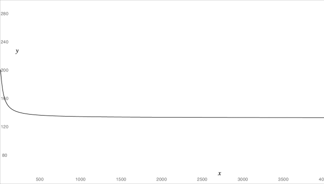
     Figure 2: For the values of $n$ ($=x$ continuous) in the interval $]7,4001]$ the function $f_{L}(x)$ decreases continuously up to the limit value of $(0,0075)^{-1}\sim 133.33\dots$

     When we fixe $d_{0}=\Lambda=0,05$ we verify (after some elementary but long manipulations) that the dominant contribution (i.e. $\sim n^{2}$) of the function :

     $$\begin{array}[]{l}f(n)=f_{L}(n)-f_{R}(n)\\ \mbox{where:}\\ f_{L}(n)=\displaystyle{\frac{(n+1)(n+2)}{1+3\Lambda(n+1)(n+2)d_{0}}(1+\frac{15}{n}+\frac{48}{n(n-1)})}\ \ \ \mbox{and}\\ f_{R}(n)=\displaystyle{\frac{n(n-1)}{1+3\Lambda n(n-1)d_{0}}(1+\frac{15}{(n-2)}+\frac{48}{(n-2)(n-3)})}\\ \mbox{is strictly negative}\\ \end{array}$$ (5.94)

     More precisely we find:

     $$\begin{array}[]{l}f(n)=2(2n+1)+\displaystyle{\frac{30n[1-2/n-2/n^{2}]}{n-2}-\frac{192n[2-2/n-3/n^{2}]]}{(n-1)(n-2)(n-3)}}-\\ -0.0075\displaystyle{\frac{30n^{2}(n+1)(n+2)}{(n-2)(n-3)}}[1+72/30n-198/30n^{2}]\end{array}$$ (5.95)

     Of course, an analogous result is also obtained if we consider that $n=x$ (as a continuous variable). The derivative of the left hand side of the inequality 5.93 is negative when we fixe $d_{0}\sim\Lambda\leq 0.05$ and for $x>7$.

     In figure 2 we graphically illustrate the behaviour of the function:

     $$f_{L}(n)=\displaystyle{\frac{(n+1)(n+2)}{1+3\Lambda(n+1)(n+2)d_{0}}(1+\frac{15}{n}+\frac{48}{n(n-1)})}$$

     We notice that when $n=x$ varies continuously from $x=7$ up to $x=4001$, $f_{L}(n)$ decreases continuously up to the limit value of $(0.15\times 0.05=0,0075)^{-1}\sim 133.33\dots$. This ends the proof of proposition 3.2.    $\blacksquare$

3. Proof of proposition 3.3

   • As previously, the sign property is directly obtained by the hypothesis $H\in\ \Phi_{0}$:

     $$\begin{array}[]{l}B^{n+1}(\Lambda)=\,-3\Lambda\displaystyle{\sum_{\varpi_{n}(J)}{n\ !\over j_{1}!j_{2}!}H^{j_{2}+2}(\Lambda)H^{j_{1}+1}(\Lambda)}=\\ =-3\Lambda\displaystyle{\sum_{\varpi_{n}(J)}{n\ !\over j_{1}!j_{2}!}(-1)^{\frac{j_{2}}{2}}|H^{j_{2}+2}|(-1)^{\frac{j_{1}-1}{2}}|H^{j_{1}+1}|}\\ =(-1)^{\frac{n-3}{2}}|B^{n+1}|\ \ \blacksquare\end{array}$$ (5.96)

   • In order to ensure the increase property we show that:

     $${\frac{|B^{n+1}_{min}|}{n(n-1)|H^{n+1}_{min}|}}>\ \displaystyle{\frac{|B^{n-1}_{min}|}{(n-2)(n-3)|H^{n-1}_{min}|}}$$ (5.97)

     The left hand side of 5.97 can be expressed in terms of the smaller contribution $B^{n+1}_{(j_{1},j_{2}),min}$ (with $j_{1}=\frac{n-1}{2},\ j_{2}=\frac{n+1}{2}$) times the number of different partitions $\varpi_{n}(J)$ in the sum of $B^{n+1}_{min}$ $\it{i.e.}\frac{n-1}{2}$; in other words:

     $$\frac{n-1}{2}B^{n+1}_{(j_{1}=\frac{n-1}{2},j_{2}=\frac{n+1}{2})}$$

     Reminder:

     $$B^{n+1}_{(j_{1}=\frac{n-1}{2},j_{2}=\frac{n+1}{2})}=\displaystyle{{n!H^{(j_{1}+1)}H^{(j_{2}+2)}\over((n-1)/2)!((n+1)/2)!}}$$

     In a similar way the r.h.side $B^{n-1}_{min}$ can be substituted by

     $$\frac{n-3}{2}B^{n-1}_{(j_{1}=\frac{n-1}{2},j_{2}=\frac{n-3}{2})}$$

     So, by taking into account the definitions of the splitting sequences and Green’s functions in $\Phi_{0}$ 2.8, 2.5, as well as proposition 2.2 (upper bounds of tree terms $C^{n+1}$ we require in a equivalent way (after some elementary simplifications) the sufficient condition:

     $$\begin{array}[]{l}\displaystyle{\frac{4\delta_{\frac{n+5}{2},min}{\mathcal{T}}_{\frac{n+5}{2}}(n-2)}{\delta_{n,min}{\mathcal{T}}_{n}^{\prime}(n+1)}}>\ 1\\ \\ \mbox{or using the definitions of $\delta^{\prime}s$ and ${\mathcal{T}}_{n}^{\prime}s$ we require the following stronger condition:}\\ \\ f_{B}=\frac{(n-2)(n+5)(n+3)[1+3\Lambda n(n-1)][(n-1)^{2}+64(n-1)+192]}{(n+1)[4+3\Lambda(n+5)(n+3)]n(n-1)[(n-3)^{2}+16(n-3)+48]}>\ 1\end{array}$$ (5.98)

     The difference between the numerator and the denominator of $f_{B}$, let us say $Num_{fB}-Den_{fB}$, is a polynomial with positive coefficients of the dominant contributions:

     $$Num_{fB}-Den_{fB}\ \sim({\cal O}(n^{7})+{\cal O}(n^{6})+{\cal O}(n^{5}))>0$$

     Another way to be convinced that the condition 5.98 is verified is to put $n=x$ (continuous) and represent graphically the function $f_{B}(x)$ at fixed $\Lambda=0.05$. The figure 3 shows precisely that $f_{B}$ decreases continuously always from larger values than $1$ up to the limit value of $1$. This ends the proof of proposition 3.3   $\blacksquare$

   

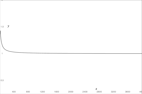
   Figure 3: For the values of $n$ ($=x$ continuous) in the interval $]7,4001]$ $f_{B}$ decreases continuously always from bigger values than $1$ up to the limit value of $1$

4. Proof of proposition 3.4

   i) Using the hypothesis $H\in\Phi$ we obtain the limit:

   $${\lim_{\Lambda\rightarrow 0}D_{n}(\Lambda)}=0\quad\forall n\geq 7$$

   ii)The increasing property is a direct consequence of the previous propositions 3.2, 3.3.

   iii) The lower and upper bounds together with the limit at infinity are also consequences of the same propositions.

2 Proof of theorem 3.1

i. 2.36 For $n=1,3,5$: the limit properties (with respect to $\Lambda$) of the $H^{2},H^{4},H^{6}$ functions are ensured in view of the hypothesis $H\in\Phi$. The signs and bounds are established in proposition 3.1

ii. For $n\geq 7$ propositions 3.2, 3.3 and 3.4 yield the simple and uniform convergence at infinity together with the uniform bounds and limit properties (with respect to $\Lambda$).

In particular the lower uniform bound $d_{0}$ of $D_{n}^{\prime}s$ ensures the positivity of $\delta^{\prime}s$ and the the upper bound at infinity $\delta_{\infty}$ of $\delta_{n,max}$. Automatically the good signs and bounds are satisfied.

$$\mbox{Moreover:}\qquad\lim_{\Lambda\rightarrow 0}\,\frac{\delta_{n}^{{}^{\prime}}(\Lambda)}{\Lambda}=\lim_{\Lambda\rightarrow 0}\,\frac{3n(n-1)}{1+D_{n}(H)}$$

In view of the hypothesis $H\in\Phi$ we apply the property $\displaystyle{\lim_{\Lambda\rightarrow 0}D_{n}(\Lambda)}=0$ of proposition 3.4 and the limit at $\Lambda=0$ is obtained.

6 Appendix II

Proof of theorem 4.1

1 The completeness of $\Phi_{0}$

i.

The ball $S_{\rho}(H_{0})\subset\Phi_{0}$ is by definition a closed subspace of ${\cal B}_{c}$ which is a complete metric space with respect to the topology defined in terms of the norm ${\cal N}$ (cf. 4.81). Consequently $S_{\rho}(H_{0})$ is also complete with respect to the induced topology.   $\blacksquare$.

In the numerical study of [14] we have precisely realized this last result:

The solution is obtained iteratively in the neighborhood of this particular sequence $H_{0}$ by using two starting points: the sequences $\{\delta_{n,max}\}$ and $\{\delta_{n,min}\}$.

Let us now present the proof of the analogous result “theoretically”.

2 The local contractivity

In this part of the paper we have to show that for every $H$ in $S_{\rho}(H_{0})$ and when $\Lambda\in]0,0.45]$ there exist two real positive constants (continuous functions of $\Lambda$), $k^{(0)}<1$ and $k<1$ with

$$k^{(0)}(\Lambda)<(1-k(\Lambda))$$

such that:

$$\begin{array}[]{l}\|\mathcal{M}^{*}(H)-H_{(0)}\|\ \leq\ k(\Lambda)\ \rho\\ \mbox{and}\\ \|\mathcal{M}^{*}(H_{0})-H_{(0)}\|\ \leq\ k^{(0)}(\Lambda)\ \rho\end{array}$$ (6.99)

By the definition 4.81  of the norm $\mathcal{N}$ the above inequalities are equivalent to the following:

$$\begin{array}[]{l}\forall\ \ \ \Lambda\in]0,0.45]\\ \qquad\qquad\displaystyle{\sup_{(n,\Lambda)}}\displaystyle{\frac{|H^{n+1^{\prime}}-H_{(0)}^{n+1}|}{M_{n}}}\leq\ k(\Lambda)\ \rho\\ \mbox{and}\\ \qquad\qquad\displaystyle{\sup_{(n,\Lambda)}}\displaystyle{\frac{|H_{(0)}^{n+1^{\prime}}-H_{(0)}^{n+1}|}{M_{n}}}\leq\ k^{(0)}(\Lambda)\ \rho\end{array}$$ (6.100)

By using definitions 2.6 (of the sequence $\{H_{0}\}$), 4.81  (of the norm $\mathcal{N}$) and for $H\in S_{\rho}$, we obtain successively:

1. for $n=1$

   $$|H^{2^{\prime}}(\Lambda)-H_{(0)}^{2}(\Lambda)|\leq\Lambda|H^{4}-H_{(min)}^{4}|\leq\Lambda[|H^{4}-H_{(0)}^{4}|+|H_{(0)}^{4}-H_{(min)}^{4}|]$$

   $$\leq 12\Lambda^{2}M_{1}^{3}\rho$$ (6.101)

   and, we write :

   $$\frac{|H^{2^{\prime}}(\Lambda)-H_{(0)}^{2}(\Lambda)|}{M_{1}(\Lambda)}\leq k_{1}(\Lambda)\rho$$ (6.102)

   where we define :

   $$k_{1}(\Lambda)=12\Lambda^{2}M_{1}^{2}$$ (6.103)

   Moreover:

   $$|H_{(0)}^{2^{\prime}}(\Lambda)-H_{(0)}^{2}(\Lambda)|\leq\Lambda|H_{(0)}^{4}-H_{(min)}^{4}|\leq 6\Lambda^{2}M_{1}^{3}\rho$$ (6.104)

   and, we write :

   $$\frac{|H(0)^{2^{\prime}}(\Lambda)-H_{(0)}^{2}(\Lambda)|}{M_{1}(\Lambda)}\leq k_{1}^{(0)}(\Lambda)\rho$$ (6.105)

   where we define :

   $$k_{1}^{(0)}(\Lambda)=6\Lambda^{2}M_{1}^{2}$$ (6.106)

   We verify that

   $$k_{1}^{(0)}(\Lambda)+k_{1}(\Lambda)<1\ \ \ \forall\ \Lambda\leq 0.1$$ (6.107)

2. For $n=3$ (in view of the definition 3.1 of ${\cal M}^{*}$) we have :

   $$|H^{4{}^{\prime}}(\Lambda)-H_{(0)}^{4{}}(\Lambda)|\leq|\delta_{3}^{\prime}-\delta_{3(0)}|(H^{2{}^{\prime}})^{3}+\delta_{3(0)}|(H^{2{}^{\prime}})^{3}-(H_{(0)}^{2})^{3}|$$ (6.108)

   and,

   $$|\delta_{3}^{\prime}-\delta_{3(0)}|\leq\frac{6\Lambda|D_{3}-D_{3(min)}|}{(1+D_{3})(1+D_{3(min)})}$$ (6.109)

   Here, from definition 2.6:

   $$D_{3(min)}=9\Lambda H^{2}_{min}-\displaystyle{\frac{\Lambda|H^{6}_{min}|}{|H^{4}_{max}|}.}$$

   So,

   $$|\delta_{3}^{\prime}-\delta_{3(0)}|\leq\frac{54\Lambda^{2}\{|H^{2}-H^{2}_{min}|-\Lambda(\frac{|H^{6}|}{|H^{4}|}-\ \frac{|H^{6}_{min}|}{|H^{4}_{max}|})\}}{(1+D_{3})(1+D_{3(min)})}$$ (6.110)

   Now in view of the bounds and sign properties of the Green’s functions inside $\Phi_{0}$, the second term on the numerator is positive and can be eliminated, precisely:

   $$(\frac{|H^{6}|}{|H^{4}|}-\ \frac{|H^{6}_{min}|}{|H^{4}_{max}|})=\displaystyle{|\frac{|H^{6}|}{|H^{4}|}-\ \frac{|H^{6}_{min}|}{|H^{4}_{max}|}|}$$ (6.111)

   Moreover:

   $$\frac{6\Lambda}{1+D_{3}}\leq\delta_{3,max}\quad\mbox{and}\quad\frac{6\Lambda}{1+D_{3(min)}}\leq\delta_{3,max}.$$

   Finally the first term on the right hand sight (r. h.s.) of 6.108 yields:

   $$|\delta_{3}^{\prime}-\delta_{3(0)}|(H^{2{}^{\prime}})^{3}\leq 3M_{1}^{4}(\delta_{3,max})^{2}\rho$$ (6.112)

   Taking into account the previous results 6.105, 6.106 for $n=1$, the second term on the r.h.s. of 6.113 yields:

   $$\delta_{3(0)}|(H^{2{}^{\prime}})^{3}-(H_{(0)}^{2})^{3}|\leq 3k_{1}(\Lambda^{2})M_{1}^{3}\delta_{3(max)}$$ (6.113)

   From the above results and the norm definition we have:

   $${\frac{|H^{4{}^{\prime}}(\Lambda)-H_{(0)}^{4{}}|}{M_{3}}}\leq k_{3}(\Lambda)\rho$$ (6.114)

   with:

   $$k_{3}(\Lambda)=9\Lambda M_{1}(1+4\Lambda)$$ (6.115)

   In an analogous way we obtain:

   $${\frac{|H_{(0)}^{4{}^{\prime}}-H_{(0)}^{4{}}|}{M_{3}}}\leq k_{3}^{(0)}(\Lambda)\rho$$ (6.116)

   with:

   $$k_{3}^{(0)}(\Lambda)=9\Lambda\displaystyle{\frac{(H_{(0)}^{2})^{2}(1+2\Lambda)}{M_{1}^{2}}}$$ (6.117)

   We finally verify that:

   $$\forall\ \ 0<\Lambda\leq 0.045\qquad k_{3}(\Lambda)+k_{3}^{(0)}(\Lambda)<1$$ (6.118)

3. For $n=5$ using the definition 3.1 of the mapping we have:

   $$|H^{6{}^{\prime}}(\Lambda)-H_{(0)}^{6{}}(\Lambda)|\leq\displaystyle{\frac{|\delta_{5}^{\prime}-\delta_{5(0)}||C^{6\prime}|}{60\Lambda}}+\displaystyle{\frac{\delta_{5(0)}|C^{6\prime}-C_{(0)}^{6}|}{60\Lambda}.}$$ (6.119)

   In view of the stability of $\Phi_{0}$, definitions 2.6 and 4.81 (of the norm), the first term of the r.h.s. of the latter yields:

   $$\begin{array}[]{c}\displaystyle{\frac{|\delta_{5}^{\prime}-\delta_{5(0)}||C^{6\prime}|}{60\Lambda}}\leq|\delta_{5(max)}-\delta_{5(min)}||H_{(max)}^{4{}}|(H_{(max)}^{2{}})^{2}\\ \leq\delta_{5(max)}M_{3}M_{1}^{2}\rho\end{array}$$ (6.120)

   By the earlier results for $n=1\ \mbox{and}\ \ n=3$, the second term of the r.h.s. of 6.119 reads:

   $${\frac{\delta_{5(0)}|C^{6\prime}-C_{(0)}^{6{}}|}{60\Lambda}}\leq\delta_{5(max)}M_{3}M_{1}^{2}\rho[k_{3}(\Lambda)+2k_{1}(\Lambda^{2})]$$ (6.121)

   Then, from 6.120, 6.121 and the norm definition 4.81 ($M_{5}=20M_{3}M_{1}^{2}\delta_{5(max)}$), we have:

   $$\begin{array}[]{l}|H^{6{}^{\prime}}(\Lambda)-H_{(0)}^{6{}}(\Lambda)|\leq\rho\ k_{5}(\Lambda)\\ \mbox{ where:}\quad k_{5}(\Lambda)=\displaystyle{\frac{1}{20}(1+k_{3}(\Lambda)+2k_{1}(\Lambda^{2}))}\end{array}$$ (6.122)

   In an analogous way we find:

   $$\begin{array}[]{l}|H^{6{(0)}^{\prime}}(\Lambda)-H_{(0)}^{6{}}(\Lambda)|\leq\rho\ k_{5}^{(0)}(\Lambda)\\ \mbox{ where:}\quad k_{5}^{0)}(\Lambda)=\displaystyle{\frac{1}{20}(1+k_{3}^{(0)}(\Lambda)+2k_{1}^{(0)}(\Lambda^{2}))}\end{array}$$ (6.123)

   and, verify that under the same condition on the coupling constant as that imposed previously in the case $n=3$ we obtain:

   $$\forall\ \ 0<\Lambda\leq 0.045\qquad k_{5}(\Lambda)+k_{5}^{(0)}(\Lambda)=0,25<1$$ (6.124)

   consequently for $n=5$ we require a weaker condition on $\Lambda.\ \ \qquad\ \qquad\blacksquare$.

4. For $n\geq 7$, we proceed by recursion :

   h.c.r: We suppose that for every $m\leq n-2$ there exist two finite positive constants (continuous functions of $\Lambda$) $k_{m}(\Lambda)$ and $k_{m}^{(0)}(\Lambda)$ precisely given by:

   $$\begin{array}[]{l}k_{m}(\Lambda)=a_{1}\displaystyle{\sum_{j=0}^{\frac{m-5}{2}}(\frac{1}{12})^{j}+(\frac{1}{(12)})^{\frac{m-5}{2}}}k_{5};\\ k_{m}^{(0)}(\Lambda)=a_{0}\displaystyle{\sum_{j=0}^{\frac{m-5}{2}}(\frac{1}{12})^{j}+(\frac{1}{12})^{\frac{m-5}{2}}k_{5}^{(0)}}\\ \mbox{with:}\quad a_{0}=\displaystyle{\frac{1}{12}+\frac{k_{1}^{(0)}(\Lambda^{2})}{6}}\ \quad\mbox{and}\quad a_{1}=\displaystyle{\frac{1}{12}+\frac{k_{1}(\Lambda^{2})}{6}}\end{array}$$ (6.125)

   such that:

   $$\begin{array}[]{l}\qquad\qquad\forall\ \Lambda\in]0,0.45]\\ \\ \qquad\qquad\displaystyle{\frac{|H^{m+1^{\prime}}-H_{(0)}^{m+1}|}{M_{n}}}\leq\ k_{m}(\Lambda)\ \rho\\ \mbox{and},\\ \qquad\qquad\displaystyle{\frac{|H_{(0)}^{m+1^{\prime}}-H_{(0)}^{m+1}|}{M_{n}}}\leq\ k_{m}^{(0)}(\Lambda)\ \rho\\ \mbox{ with:}\\ \qquad\qquad k_{m}(\Lambda)+k_{m}^{(0)}(\Lambda)\ <\ 1\end{array}$$ (6.126)

   We establish the statement  h.c.r for $m=n$ by using arguments analogous to that for $m=5$:

   By the definition 3.1 of the mapping we have:

   $$|H^{n+1{}^{\prime}}-H_{(0)}^{n+1{}}(\Lambda)|\leq\displaystyle{\frac{|\delta_{n}^{\prime}-\delta_{n(0)}||C^{n+1\prime}|}{3\Lambda n(n-1)}}+\displaystyle{\frac{\delta_{n(0)}|C^{n+1\prime}-C_{(0)}^{n+1}|}{3\Lambda n(n-1)}.}$$ (6.127)

   In view of the stability of $\Phi_{0}$, definitions 2.6 and 4.81 (of the norm), the first term of the r.h.s. of the latter yields:

   $$\begin{array}[]{c}\displaystyle{\frac{|\delta_{n}^{\prime}-\delta_{n(0)}||C^{n+1\prime}|}{3\Lambda n(n-1)}}\leq|\delta_{n(max)}-\delta_{n(min)}|\ \mathcal{T}_{n}\ |H_{(max)}^{n-1{}}|(H_{(max)}^{2{}})^{2}\\ \leq\delta_{n(max)}\ {\mathcal{T}_{n}}\ M_{n-2}M_{1}^{2}\rho\end{array}$$ (6.128)

   Here we have taken into account the bound of the tree term $C^{n+1\prime}$ given by Proposition 2.2 in terms of the dominant contribution $|H_{(max)}^{n-1{}}|(H_{(max)}^{2{}})^{2}$.

   $\mathcal{T}_{n}$ means the number of different partitions in the sum $\sum\limits_{\varpi_{n}(I)}$ of the tree term (cf. App. A of reference [2, c]) which verifies :
   

   $$\forall\ \ \ n>9,\qquad\mathcal{T}_{n}=\frac{(n-3)^{2}}{48}+\frac{(n-3)}{3}+1,$$ (6.129)

   Remark 6.1

   We remind that $\mathcal{T}_{7}=2$ and $\mathcal{T}_{9}=3$ because only the two last terms in the expression 6.129 yield a nontrivial contribution.

   By the recurrence hypothesis for $n-2\ \mbox{and the earlier result for }\ \ n=1$, the second term of the r.h.s. of 6.127 (tree term) yields:

   $${\frac{\delta_{n(0)}|C^{n+1\prime}-C_{(0)}^{n+1}|}{3\Lambda n(n-1)}}\leq\delta_{n(max)}\mathcal{T}_{n}\ M_{n-2}M_{1}^{2}\rho[k_{n-2}(\Lambda)+2k_{1}(\Lambda^{2})]$$ (6.130)

   Then, from 6.128, 6.129, 6.130 the norm definition 4.81:

   $$M_{n}=n(n-1)M_{n-2}M_{1}^{2}\delta_{n(max)},$$

   and the bound:

   $${\frac{1}{48n(n-1)}[(n-3)^{2}]+16(n-3)+48]<\ \frac{4}{48}=\frac{1}{12}}\ \qquad\forall n\geq 7)$$

   we obtain:

   $$\begin{array}[]{l}|H^{n+1{}^{\prime}}(\Lambda)-H_{(0)}^{n+1{}}(\Lambda)|\leq\rho\ k_{n}(\Lambda)\\ \mbox{ where:}\quad k_{n}(\Lambda)=\displaystyle{\frac{1}{12}+\frac{k_{n-2}}{12}+\frac{k_{1}(\Lambda^{2})}{6}}\end{array}$$ (6.131)

   In an analogous way we find:

   $$\begin{array}[]{l}|H_{(0)}^{n+1{}^{\prime}}(\Lambda)-H_{(0)}^{n+1{}}(\Lambda)|\leq\rho\ k_{n}^{(0)}(\Lambda)\\ \mbox{ where:}\quad k_{n}^{(0)}(\Lambda)=\displaystyle{\frac{1}{12}+\frac{k_{n-2}^{(0)}}{12}+\frac{k_{1}{(0)}(\Lambda^{2})}{6}}\end{array}$$ (6.132)

   Now, by the expression of he recursion statement h.c.r 6.125 for $k_{n-2}$ and respectively for $k_{n-2}^{(0)}$ we obtain:

   $$\begin{array}[]{l}k_{n}(\Lambda)=\displaystyle{\frac{1}{12}+\frac{1}{12}a_{1}\displaystyle{\sum_{j=0}^{\frac{n-7}{2}}(\frac{1}{12})^{j}+(\frac{1}{12})^{\frac{n-7}{2}}k_{5}}+\frac{k_{1}(\Lambda^{2})}{6}}=\\ =a_{1}\displaystyle{\sum_{j=0}^{\frac{n-5}{2}}(\frac{1}{12})^{j}+(\frac{1}{12})^{\frac{n-5}{2}}k_{5}}\\ \mbox{and respectively,}\\ k_{n}^{(0)}(\Lambda)=a_{0}\displaystyle{\sum_{j=0}^{\frac{n-5}{2}}(\frac{1}{12})^{j}+(\frac{1}{12})^{\frac{n-5}{2}}k_{5}^{(0)}}\end{array}$$ (6.133)

   We directly verify that:

   $$\forall\ \ \ \Lambda\in]0,0.45]\quad k_{n}(\Lambda)+k_{n}^{(0)}(\Lambda)\ <1$$ (6.134)

   This result ends the proof of the recursive formula    $\qquad\qquad\blacksquare$

   Finally, taking into account the limit of the convergent geometric series in the final results 6.133 we also verify that:

   $$\begin{array}[]{l}\displaystyle{\sup_{n}\ k_{n}(\Lambda)=\ \lim_{n\to\infty}\{\ a_{1}\sum_{j=0}^{\frac{n-5}{2}}(\frac{1}{12})^{j}+(\frac{1}{12})^{\frac{n-5}{2}}k_{5}}\}=\\ =\frac{1}{11}+\frac{k_{1}(\Lambda^{2})}{6}\end{array}$$ (6.135)

   and by analogy:

   $$\begin{array}[]{l}\displaystyle{\sup_{n}\ k_{n}^{(0)}(\Lambda)=\ \lim_{n\to\infty}\{\ a_{1}\sum_{j=0}^{\frac{n-5}{2}}(\frac{1}{12})^{j}+(\frac{1}{12})^{\frac{n-5}{2}}k_{5}}\}=\\ =\frac{1}{11}+\frac{k_{1}^{(0)}(\Lambda^{2})}{6}\end{array}$$ (6.136)

   Then we introduce:

   $$\begin{array}[]{l}k=\displaystyle{\sup_{(n;\Lambda\in]0,0.045])}(k_{n}(\Lambda)}\\ \mbox{and in a similar way}\\ k^{(0)}=\displaystyle{\sup_{(n;\Lambda)}k_{n}^{(0)}(\Lambda)}\end{array}$$ (6.137)

   By the definitions 6.103, 6.106 of $k_{1}(\Lambda^{2})$ and $k_{1}^{(0)}(\Lambda^{2})$ we find:

   $$k=\frac{1}{11}+0.005=0.096;\ \ \ \mbox{and}\ \ k^{(0)}=0.094$$ (6.138)

   Conclusion:

   $$\begin{array}[]{l}\forall\ \ \ \Lambda\in]0,0.45]\\ \qquad\qquad\displaystyle{\sup_{(n,\Lambda)}}\displaystyle{\frac{|H^{n+1^{\prime}}-H_{(0)}^{n+1}|}{M_{n}}}\leq\ k\ \rho\\ \mbox{and}\\ \qquad\qquad\displaystyle{\sup_{(n,\Lambda)}}\displaystyle{\frac{|H_{(0)}^{n+1^{\prime}}-H_{(0)}^{n+1}|}{M_{n}}}\leq\ k^{(0)}\ \rho\\ \mbox{with:}k+k^{(0)}<1\qquad\qquad\ \ \blacksquare\end{array}$$ (6.139)