Equation of state for magnetized Coulomb plasmas

We have developed an analytical equation of state (EOS) for magnetized fully-ionized plasmas that cover a wide range of temperatures and densities, from low-density classical plasmas to relativistic, quantum plasma conditions. This EOS directly applies to calculations of structure and evolution of strongly magnetized white dwarfs and neutron stars. We review available analytical and numerical results for thermodynamic functions of the nonmagnetized and magnetized Coulomb gases, liquids, and solids. We propose a new analytical expression for the free energy of solid Coulomb mixtures. Based on recent numerical results, we have constructed analytical approximations for the thermodynamic functions of harmonic Coulomb crystals in quantizing magnetic fields. The analytical description ensures a consistent evaluation of all astrophysically important thermodynamic functions based on the first, second, and mixed derivatives of the free energy. Our numerical code for calculation of thermodynamic functions based on these approximations has been made publicly available. Using this code, we calculate and discuss the effects of electron screening and magnetic quantization on the position of the melting point in a range of densities and magnetic fields relevant to white dwarfs and outer envelopes of neutron stars. We consider also the thermal and mechanical structure of a magnetar envelope and argue that it can have a frozen surface which covers the liquid ocean above the solid crust.

1 Introduction

Coulomb plasmas, i.e., the fully-ionized plasmas whose thermodynamics is strongly affected by electrostatic interactions, are encountered in many physical and astrophysical situations (e.g., Fortov 2009). Full ionization is reached either at high temperatures $T$ and low densities $\rho$ (thermal ionization) or at high densities $\rho$ (pressure ionization). The latter case is typical of the interior conditions of low-mass stars, brown dwarfs, or giant planets (Chabrier & Baraffe 2000) as well as the interior and envelope conditions of white dwarfs and neutron stars. Coulomb interactions are crucial for the equation of state (EOS) under such conditions. In the interior or the envelope of compact objects such as white dwarfs and neutron stars, the electrons can be weakly or strongly degenerate, the plasma can be in the liquid or solid state, the electrons can have various degrees of degeneracy and relativism, and the quantum effects on ion motion can be substantial. Therefore, a wide-range EOS is needed for calculations of the structure and evolution of such stars.

In a previous work (Potekhin & Chabrier 2000, 2010, hereafter Paper I and Paper II, respectively) we proposed a set of analytical expressions for the calculations of the EOSs of the Coulomb plasmas without magnetic fields and presented a code for thermodynamic functions based on the first, second, and mixed derivatives of the analytical Helmholtz free energy $F$ with respect to density $\rho$ and temperature $T$. This code has been employed in astrophysical modeling and adapted for the use in the Modules for Experiments in Stellar Astrophysics (MESA) (Paxton et al. 2011).

The Bohr – van Leeuwen theorem states that an EOS of charged pointlike classical particles is not affected by a magnetic field (van Leeuwen 1921). However, a magnetic field can affect thermodynamic functions through intrinsic magnetic moments of particles and by the quantization of the motion of charged particles in Landau orbitals (Landau 1930; Landau & Lifshitz 1977). These effects can be important, for example, in magnetic white dwarfs whose magnetic fields $B$ can reach $10^{7}-10^{9}$ G (e.g., Wickramasinghe & Ferrario 2000, and references therein) and neutron stars with typical $B\sim 10^{8}-10^{14}$ G (e.g., Haensel et al. 2007, and references therein).

In this paper, we systematically consider analytical expressions for thermodynamic functions of magnetized Coulomb plasmas, discuss their validity range, and introduce some practical modifications. We take account of analytical and numerical results, currently available for various contributions to the Helmholtz free energy in quantizing magnetic fields. Taking advantage of recently published numerical results (Baiko 2009), we construct an analytical description of the thermodynamic functions of harmonic Coulomb crystals in quantizing magnetic fields.

In Sect. 2 we give definitions and simple estimates for the plasma parameters that determine different thermodynamic regimes. In Sect. 3 we outline the EOS of a nonmagnetized Coulomb plasma as the reference case. In Sect. 4 we consider the Boltzmann and Fermi gases in quantizing magnetic fields, present a general analytical description of their EOS, and simplify them for several limiting cases. In Sect. 5 we review nonideal contributions to the EOS of a Coulomb liquid in a strong magnetic field. In Sect. 6 we derive an analytical approximation for the EOS of a strongly magnetized Coulomb crystal. In Sect. 7 we present and discuss examples of thermodynamic functions for conditions typical of white dwarfs and neutron-star envelopes. The summary is given in Sect. 8. In the Appendices we give the explicit expressions for the thermodynamic functions used in Sect. 3.

2 Basic definitions

2.1 General parameters

Let $n_{\mathrm{e}}$ and $n_{\mathrm{i}}$ be the electron and ion number densities, $A$ and $Z$ the ion mass and charge numbers, respectively. In this paper we consider the neutral plasmas (therefore $n_{\mathrm{e}}=Zn_{\mathrm{i}}$) that contain a single type of ion and include neither positrons (they can be described using the same analytical functions as for the electrons; see, e.g., Blinnikov et al. 1996; Timmes & Arnett 1999), nor free neutrons (see Haensel et al. 2007 for a review).

The state of a free-electron gas is determined by the electron number density $n_{\mathrm{e}}$ and temperature $T$. Instead of $n_{\mathrm{e}}$ it is convenient to introduce the dimensionless density parameter $r_{\mathrm{s}}=a_{\mathrm{e}}/a_{0}$, where $a_{0}$ is the Bohr radius and $a_{\mathrm{e}}=(\frac{4}{3}\pi n_{\mathrm{e}})^{-1/3}$. The parameter $r_{\mathrm{s}}$ can be quickly evaluated from the relations $r_{\mathrm{s}}=1.1723\,n_{24}^{-1/3}=(\rho_{0}/\rho)^{1/3},$ where $n_{24}\equiv n_{\mathrm{e}}/10^{24}{\rm\leavevmode\nobreak\ cm}^{-3}$ and $\rho_{0}=2.6752\,(A/Z)$ g cm^-3. The analogous density parameter for the ions is $R_{\mathrm{S}}=a_{\mathrm{i}}m_{\mathrm{i}}(Ze)^{2}/\hbar^{2}=1822.89AZ^{7/3}\,r_{\mathrm{s}}$, where $m_{\mathrm{i}}$ is the ion mass and $a_{\mathrm{i}}\equiv(\frac{4}{3}\pi n_{\mathrm{i}})^{-1/3}$ is the ion sphere radius.

At stellar densities it is convenient to use, instead of $r_{\mathrm{s}}$, the nonmagnetic relativity parameter

$$x_{\mathrm{r}}=p_{\mathrm{F}}/m_{\mathrm{e}}c=1.00884\,\left(\rho_{6}Z/A\right)^{1/3}\!\!=0.014005\,r_{\mathrm{s}}^{-1},$$ (1)

where $p_{\mathrm{F}}=\hbar\,(3\pi^{2}n_{\mathrm{e}})^{1/3}$ is the electron Fermi momentum in the absence of a magnetic field, and $\rho_{6}\equiv\rho/10^{6}$ g cm^-3. The Fermi energy (without the rest energy) for the electron gas is $\epsilon_{\mathrm{F}}=c\,\sqrt{(m_{\mathrm{e}}c)^{2}+(p_{\mathrm{F}})^{2}}-m_{\mathrm{e}}c^{2},$ and the Fermi temperature $T_{\mathrm{F}}\equiv\epsilon_{\mathrm{F}}/k_{\mathrm{B}}=T_{\mathrm{r}}\,(\gamma_{\mathrm{r}}-1),$ where $T_{\mathrm{r}}\equiv{m_{\mathrm{e}}c^{2}/k_{\mathrm{B}}}=5.93\times 10^{9}\leavevmode\nobreak\ \mathrm{K}$, $\gamma_{\mathrm{r}}\equiv\sqrt{1+x_{\mathrm{r}}^{2}}$, and $k_{\mathrm{B}}$ is the Boltzmann constant. A useful measure of electron degeneracy is $\theta=T/T_{\mathrm{F}}$. In the nonrelativistic limit ($x_{\mathrm{r}}\ll 1$), $T_{\mathrm{F}}\approx 1.163\times 10^{6}\,r_{\mathrm{s}}^{-2}$ K, and

$$\theta=0.543\,r_{\mathrm{s}}/\Gamma_{\mathrm{e}},$$ (2)

where

$$\Gamma_{\mathrm{e}}\equiv\frac{e^{2}}{a_{\mathrm{e}}k_{\mathrm{B}}T}\approx\frac{22.747}{T_{6}}\left(\rho_{6}\frac{Z}{A}\right)^{1/3}.$$ (3)

In the opposite ultrarelativistic limit ($x_{\mathrm{r}}\gg 1$), $\theta\approx(263\,\Gamma_{\mathrm{e}})^{-1}$. The strength of the Coulomb interaction of nonrelativistic ions is characterized by the Coulomb coupling parameter

$$\Gamma=\frac{(Ze)^{2}}{a_{\mathrm{i}}k_{\mathrm{B}}T}=\Gamma_{\mathrm{e}}Z^{5/3},$$ (4)

where $T_{6}\equiv T/10^{6}$ K.

Thermal de Broglie wavelengths of free ions and electrons are usually defined as

$$\lambda_{\mathrm{i}}=\left(\frac{2\pi\hbar^{2}}{m_{\mathrm{i}}k_{\mathrm{B}}T}\right)^{1/2},\quad\lambda_{\mathrm{e}}=\left(\frac{2\pi\hbar^{2}}{m_{\mathrm{e}}k_{\mathrm{B}}T}\right)^{1/2}\,,$$ (5)

although in some publications these definitions differ by a numerical factor. The quantum effects on ion motion are important either at $\lambda_{\mathrm{i}}\gtrsim a_{\mathrm{i}}$ or at $T\ll T_{\mathrm{p}}$, where $T_{\mathrm{p}}\equiv\hbar\omega_{\mathrm{p}}/k_{\mathrm{B}}$ is the ion plasma temperature and $\omega_{\mathrm{p}}=\left({4\pi e^{2}\,n_{\mathrm{i}}}Z^{2}/m_{\mathrm{i}}\right)^{1/2}$ is the ion plasma frequency. Since $\lambda_{\mathrm{i}}/a_{\mathrm{i}}=(T_{\mathrm{p}}/T)\sqrt{2\pi/3\Gamma}$, the importance of the quantum effects in strongly coupled plasmas (i.e., at $\Gamma\gg 1$) is determined by parameter

$$\eta\equiv T_{\mathrm{p}}/T=\Gamma\sqrt{3/R_{\mathrm{S}}}\approx 7.832\,(Z/A)\sqrt{\rho_{6}}/T_{6}.$$ (6)

2.2 Magnetic-field parameters

In the nonrelativistic theory (Landau & Lifshitz 1977), the energy of an electron in magnetic field $\bm{B}$ equals $n\hbar\omega_{\mathrm{c}}+m_{\mathrm{e}}p_{z}^{2}/2$, where $p_{z}$ is the momentum component along $\bm{B}$, $\omega_{\mathrm{c}}=eB/m_{\mathrm{e}}c$ is the electron cyclotron frequency, $n=n_{\mathrm{L}}+\frac{1}{2}-\frac{1}{2}\sigma$ characterizes a Landau level, $\sigma=\pm 1$ determines the spin projection on the field, and $n_{\mathrm{L}}$ is the non-negative integer Landau number related to the quantization of the kinetic motion transverse to the field. In the relativistic theory (Johnson & Lippmann 1949; Berestetskiĭ et al. 1982), the kinetic energy $\epsilon$ of an electron at the Landau level $n$ and its longitudinal momentum $p_{z}$ are inter-related as

$$\epsilon=\epsilon_{n}(p_{z})=c\,\left(m_{\mathrm{e}}^{2}c^{2}+2\hbar\omega_{\mathrm{c}}m_{\mathrm{e}}n+p_{z}^{2}\right)^{1/2}-m_{\mathrm{e}}c^{2},$$ (7)

$$|p_{z}|=p_{n}(\epsilon)=\left[(m_{\mathrm{e}}c+\epsilon/c)^{2}-(m_{\mathrm{e}}c)^{2}-2m_{\mathrm{e}}\hbar\omega_{\mathrm{c}}n\right]^{1/2}.$$ (8)

The levels $n\geqslant 1$ are double-degenerate with respect to $\sigma$. Their splitting due to the anomalous magnetic moment of the electron is $\approx(m_{\mathrm{e}}c^{2}\alpha_{\mathrm{f}}/2\pi)\,b$ at $b\ll 1$ and $\sim(m_{\mathrm{e}}c^{2}\alpha_{\mathrm{f}}/2\pi)\,[\ln b-1.584]^{2}$ at $b\gg 1$ (see Schwinger 1988; Suh & Mathews 2001), which is always much smaller than $\hbar\omega_{\mathrm{c}}$ and is negligible in the compact stars.

Convenient dimensionless parameters that characterize the magnetic field in a plasma are the ratios of the electron cyclotron energy $\hbar\omega_{\mathrm{c}}$ to the Hartree unit of energy, to the electron rest energy, and to $k_{\mathrm{B}}T$:

$$\gamma_{\mathrm{m}}=\hbar^{3}B/m_{\mathrm{e}}^{2}ce^{3}=B/B_{0},\quad$$ (9)

where $B_{0}=2.3505\times 10^{9}\mbox{\leavevmode\nobreak\ G}$,

$$b=\frac{\hbar\omega_{\mathrm{c}}}{m_{\mathrm{e}}c^{2}}=\alpha_{\mathrm{f}}^{2}\,\gamma_{\mathrm{m}}=\frac{B}{4.414\times 10^{13}\mbox{\leavevmode\nobreak\ G}}\,,$$ (10)

where $\alpha_{\mathrm{f}}=e^{2}/\hbar c$ is the fine-structure constant, and

$$\zeta=\hbar\omega_{\mathrm{c}}/k_{\mathrm{B}}T\approx 134.34B_{12}/T_{6},$$ (11)

where $B_{12}\equiv B/10^{12}$ G. The magnetic length $a_{\mathrm{m}}=(\hbar c/eB)^{1/2}=a_{0}/\sqrt{\gamma_{\mathrm{m}}}$ gives a characteristic transverse scale of the electron wave function.

For the ions, the cyclotron energy is $\hbar\omega_{\mathrm{ci}}=Z\,(m_{\mathrm{e}}/m_{\mathrm{i}})\,\hbar\omega_{\mathrm{c}}$, and the parameter analogous to $\zeta$ is

$$\zeta_{\mathrm{i}}=\hbar\omega_{\mathrm{ci}}/k_{\mathrm{B}}T\approx 0.0737\,(Z/A)B_{12}/T_{6}.$$ (12)

Another important parameter is the ratio of the ion cyclotron frequency to the plasma frequency,

$$\beta=\omega_{\mathrm{ci}}/\omega_{\mathrm{p}}=\zeta_{\mathrm{i}}/\eta\approx 0.0094\,B_{12}/\sqrt{\rho_{6}}.$$ (13)

2.3 Free energy and thermodynamic functions

The Helmholtz free energy $F$ of a plasma can be conveniently written as

$$F=F_{\mathrm{id}}^{\mathrm{(i)}}+F_{\mathrm{id}}^{\mathrm{(e)}}+F_{\mathrm{ee}}+F_{\mathrm{ii}}+F_{\mathrm{ie}},$$ (14)

where $F_{\mathrm{id}}^{\mathrm{(i)}}$ and $F_{\mathrm{id}}^{\mathrm{(e)}}$ denote the ideal free energy of the ions and the electrons, and the last three terms represent an excess free energy arising from the electron-electron, ion-ion, and ion-electron interactions, respectively. In the nonideal plasmas, correlations between any plasma particles depend on all interactions, therefore the separation in Eq. 14 is just a question of convenience.

An important reference case is the model of one-component plasma (OCP). In this model, the electrons are replaced by a rigid (nonpolarizable) background of the uniform charge distribution. It is convenient to define $F_{\mathrm{ii}}$ as the difference between $F$ and $F_{\mathrm{id}}^{\mathrm{(i)}}$ in the OCP model. Still stronger simplification is the ion-sphere model, in which the interaction energy in the OCP is evaluated as the electrostatic energy of a positive ion in the negatively charged sphere of radius $a_{\mathrm{i}}$ (Salpeter 1961). The electron exchange-correlation term is defined as $F_{\mathrm{ee}}=F-F_{\mathrm{id}}^{\mathrm{(e)}}$ in the model of an electron gas without consideration of the ions, which are replaced by an uniform positive background to ensure the global charge neutrality. The ion-electron (electron polarization) contribution $F_{\mathrm{ie}}$, then, is the difference between $F$ and the other terms, when interactions between all types of particles are taken into account.

The pressure $P$, the internal energy $U$, and the entropy $S$ of an ensemble of particles in volume $V$ can be found from the thermodynamic relations $P=-(\partial F/\partial V)_{T},\quad S=-(\partial F/\partial T)_{V},$ and $U=F+TS$. The second-order thermodynamic functions are derived by differentiating these first-order functions. The decomposition (Eq. 14) induces analogous decompositions of $P$, $U$, $S$, the heat capacity $C_{V}=(\partial S/\partial\ln T)_{V},$ and the logarithmic derivatives $\chi_{T}=(\partial\ln P/\partial\ln T)_{V}$ and $\chi_{\rho}=-(\partial\ln P/\partial\ln V)_{T}.$ Other second-order functions can be expressed through these functions by Maxwell relations (e.g., Landau & Lifshitz 1980).

3 EOS of nonmagnetized Coulomb plasmas

3.1 Ideal part of the free energy

The free energy of a gas of $N_{\mathrm{i}}=n_{\mathrm{i}}V$ nonrelativistic classical ions is

$$F_{\mathrm{id}}^{\mathrm{(i)}}=N_{\mathrm{i}}k_{\mathrm{B}}T\left[\ln(n_{\mathrm{i}}\lambda_{\mathrm{i}}^{3}/M_{\mathrm{spin}})-1\right],$$ (15)

where $M_{\mathrm{spin}}$ is the spin multiplicity. Accordingly, $U_{\mathrm{id}}^{\mathrm{(i)}}=\frac{3}{2}\,N_{\mathrm{i}}k_{\mathrm{B}}T$, $P_{\mathrm{id}}^{\mathrm{(i)}}=n_{\mathrm{i}}k_{\mathrm{B}}T$, $C_{V,\mathrm{id}}^{\mathrm{(i)}}=\frac{3}{2}\,N_{\mathrm{i}}k_{\mathrm{B}}$, and $\chi_{T,\mathrm{id}}^{\mathrm{(i)}}=\chi_{\rho,\mathrm{id}}^{\mathrm{(i)}}=1$. In the OCP, Eq. 15 can be written in terms of the dimensionless plasma parameters (Sect. 2) as

$$\frac{F_{\mathrm{id}}^{\mathrm{(i)}}}{N_{\mathrm{i}}k_{\mathrm{B}}T}=3\ln\eta-\frac{3}{2}\ln\Gamma-\frac{1}{2}\ln\frac{6}{\pi}-\ln M_{\mathrm{spin}}-1.$$ (16)

The free energy of the electron gas is given by

$$F_{\mathrm{id}}^{\mathrm{(e)}}=\mu_{\mathrm{e}}N_{\mathrm{e}}-P_{\mathrm{id}}^{\mathrm{(e)}}\,V,$$ (17)

where $N_{\mathrm{e}}=n_{\mathrm{e}}V$ is the number of electrons and $\mu_{\mathrm{e}}$ is the electron chemical potential without the rest energy $m_{\mathrm{e}}c^{2}$. The pressure and the number density are functions of $\mu_{\mathrm{e}}$ and $T$:

$$P_{\mathrm{id}}^{\mathrm{(e)}} = \frac{8}{3\sqrt{\pi}}\,\frac{k_{\mathrm{B}}T}{\lambda_{\mathrm{e}}^{3}}\left[I_{3/2}(\chi_{\mathrm{e}},\tau)+\frac{\tau}{2}I_{5/2}(\chi_{\mathrm{e}},\tau)\right],$$ (18)

$$n_{\mathrm{e}} = \frac{4}{\sqrt{\pi}\,\lambda_{\mathrm{e}}^{3}}\left[I_{1/2}(\chi_{\mathrm{e}},\tau)+\tau I_{3/2}(\chi_{\mathrm{e}},\tau)\right],$$ (19)

where $\chi_{\mathrm{e}}\equiv\mu_{\mathrm{e}}/k_{\mathrm{B}}T$, $\tau\equiv T/T_{\mathrm{r}}$, and

$$I_{\nu}(\chi_{\mathrm{e}},\tau)\equiv\int_{0}^{\infty}\frac{x^{\nu}\,(1+\tau x/2)^{1/2}}{\exp(x-\chi_{\mathrm{e}})+1}\,{\mathrm{d}}x$$ (20)

is the Fermi-Dirac integral. The internal energy is

$$U_{\mathrm{id}}^{\mathrm{(e)}}=\frac{4}{\sqrt{\pi}}\,\frac{k_{\mathrm{B}}TV}{\lambda_{\mathrm{e}}^{3}}\left[I_{3/2}(\chi_{\mathrm{e}},\tau)+\tau\,I_{5/2}(\chi_{\mathrm{e}},\tau)\right].$$ (21)

Since we use $V$ and $T$ as independent variables, we need to find $\mu_{\mathrm{e}}(V,T)$. This can be done either by inverting Eq. 19 numerically, or from the analytical approximation given in Chabrier & Potekhin (1998). Then the second-order thermodynamic functions are obtained using relations of the type

$$\left(\frac{\partial f(\chi_{\mathrm{e}},T)}{\partial T}\right)_{V}=\left(\frac{\partial f}{\partial T}\right)_{\!\chi_{\mathrm{e}}}\!\!-\left(\frac{\partial f}{\partial\chi_{\mathrm{e}}}\right)_{T}\,\frac{(\partial n_{\mathrm{e}}/\partial T)_{\chi_{\mathrm{e}}}}{(\partial n_{\mathrm{e}}/\partial\chi_{\mathrm{e}})_{T}},\hskip 15.00002pt$$ (22)

$$\left(\frac{\partial f(\chi_{\mathrm{e}},T)}{\partial V}\right)_{T}\!\!=-\frac{n_{\mathrm{e}}}{V}\left(\frac{\partial f}{\partial n_{\mathrm{e}}}\right)_{T}\!\!=-\frac{n_{\mathrm{e}}}{V}\,\frac{(\partial f/\partial\chi_{\mathrm{e}})_{T}}{(\partial n_{\mathrm{e}}/\partial\chi_{\mathrm{e}})_{T}}.\hskip 15.00002pt$$ (23)

We use analytical approximations for $I_{\nu}(\chi_{\mathrm{e}},\tau)$ based on the fits of Blinnikov et al. (1996) and accurate typically to a few parts in $10^{4}$, with maximum error $<0.2$% at $\tau\leq 100$ (Chabrier & Potekhin 1998). These approximations are given by different expressions in three ranges of $\chi_{\mathrm{e}}$: below, within, and above the interval $0.6\leq\chi_{\mathrm{e}}<14$. In particular, at large $\chi_{\mathrm{e}}$ the Sommerfeld expansion (e.g., Chandrasekhar 1957; Girifalco 1973) yields

$$I_{\nu}(\chi_{\mathrm{e}},\tau)=\frac{1}{\sqrt{2}\,\tau^{\nu+1}}\left(\mathcal{I}_{\nu}^{(0)}(\tilde{\mu})+\frac{\pi^{2}}{6}\,\tau^{2}\mathcal{I}_{\nu}^{(2)}(\tilde{\mu})+\ldots\right),$$ (24)

where $\tilde{\mu}\equiv\chi_{\mathrm{e}}\tau=\mu_{\mathrm{e}}/m_{\mathrm{e}}c^{2}$ is the electron chemical potential (without the rest energy) in the relativistic units,

$$\mathcal{I}_{1/2}^{(0)}(\tilde{\mu})=[\tilde{x}\tilde{\gamma}-\ln(\tilde{x}+\tilde{\gamma})]/2,$$ (25)

$$\mathcal{I}_{3/2}^{(0)}(\tilde{\mu})=\tilde{x}^{3}/3-\mathcal{I}_{1/2}^{(0)}(\tilde{\mu}),$$ (26)

$$\mathcal{I}_{5/2}^{(0)}(\tilde{\mu})=\tilde{x}^{3}\tilde{\gamma}/4-2\tilde{x}^{3}/3+1.25\,\mathcal{I}_{1/2}^{(0)}(\tilde{\mu}),$$ (27)

$$\mathcal{I}_{\nu}^{(n+1)}(\tilde{\mu})={\mathrm{d}\mathcal{I}_{\nu}^{(n)}}/{\mathrm{d}\tilde{\mu}}.$$ (28)

Here, we have introduced notations $\tilde{x}\equiv\sqrt{\tilde{\mu}(2+\tilde{\mu})}$ and $\tilde{\gamma}\equiv\sqrt{1+\tilde{x}^{2}}=1+\tilde{\mu}$. At strong degeneracy, $\tilde{\mu}\approx\epsilon_{\mathrm{F}}/m_{\mathrm{e}}c^{2}-1$, $\tilde{x}\approx x_{\mathrm{r}}$, and $\tilde{\gamma}\approx\gamma_{\mathrm{r}}$. In Paper II we also described an alternative expansion in powers of $\tau$, which allows one to avoid numerical cancellations of close terms at small $\tilde{\mu}$ (we switch to this alternative expansion at $\tilde{\mu}<0.1$).

The discontinuities of the Blinnikov et al. (1996) approximations for $I_{\nu}(\chi_{\mathrm{e}},\tau)$ at $\chi_{\mathrm{e}}=0.6$ and $\chi_{\mathrm{e}}=14$ are typically a few parts in $10^{4}$ at $\tau\lesssim 10^{2}$, but they may reach $\approx 1$% for the second derivatives. This accuracy is sufficient for many applications. Nevertheless, the jumps may produce problems, e.g., when higher derivatives are evaluated numerically in a stellar evolution code. In our calculations of white-dwarf evolution (to be published elsewhere), we smoothly interpolate between the two analytical approximations for the adjacent intervals near the boundary at the cost of a slight violation of the thermodynamic consistency in the interpolation regions (this version of the EOS code is now also available at our web site).

If a higher accuracy is needed, one can numerically calculate tables of $I_{\nu}(\chi_{\mathrm{e}},\tau)$ (e.g., Timmes & Arnett 1999) and interpolate in them with an algorithm that preserves thermodynamic consistency (Timmes & Swesty 2000) and is available at MESA (Paxton et al. 2011).

3.2 Nonideal contributions

3.2.1 Electron and ion liquids

The contribution to the free energy due to the electron-electron interactions has been studied by many authors. For the reasons explained in Paper II, we adopt the fit to $F_{\mathrm{ee}}$ derived by Ichimaru et al. (1987) (see Appendix A).

The ion-ion interactions are described using the OCP model. In the liquid regime, the numerical results obtained for the OCP of nonrelativistic pointlike charged particles in different intervals of the Coulomb coupling parameter from $\Gamma=0$ to $\Gamma\sim 200$ by different numerical and analytical methods are reproduced by a simple expression given in Appendix B.1. The accurate fit for classical OCP is supplemented by the Wigner-Kirkwood correction, which extends the applicability range of our approximations to lower temperatures $T\sim T_{\mathrm{p}}$. In spite of the significant progress in numerical ab initio modeling of quantum ion liquids, available results do not currently allow us to establish an analytical extension to still lower temperatures $T\ll T_{\mathrm{p}}$ (see Chabrier et al. 2002, for references and discussion).

3.2.2 Coulomb crystal

At $T<T_{\mathrm{m}}$, where $T_{\mathrm{m}}$ is the melting temperature, the ions in thermodynamic equilibrium are arranged in the body-centered cubic (bcc) Coulomb lattice. In the harmonic approximation (e.g., Kittel 1963), the free energy of the lattice is

$$F_{\mathrm{lat}}=U_{0}+U_{\mathrm{q}}+F_{\mathrm{th}},$$ (29)

where $U_{0}=N_{\mathrm{i}}C_{0}(Ze)^{2}/a_{\mathrm{i}}$ is the classical static-lattice energy, $C_{0}\approx-0.9$ is the Madelung constant,

$$U_{\mathrm{q}}=\frac{3}{2}N_{\mathrm{i}}\hbar\omega_{\mathrm{p}}u_{1}$$ (30)

accounts for zero-point quantum vibrations, $u_{1}=\langle\omega_{\bm{k}\alpha}\rangle_{\mathrm{ph}}/\omega_{\mathrm{p}}\approx 0.5$ is the reduced first moment of phonon frequencies,

$$F_{\mathrm{th}}=3N_{\mathrm{i}}k_{\mathrm{B}}T\left\langle\ln[1-\exp(-\hbar\omega_{\bm{k}\alpha}/k_{\mathrm{B}}T)]\right\rangle_{\mathrm{ph}}$$ (31)

is the thermal contribution, $\omega_{\bm{k}\alpha}$ are phonon frequencies, and $\langle\ldots\rangle_{\mathrm{ph}}$ denotes the averaging over phonon polarizations $\alpha$ and wave vectors $\bm{k}$ in the first Brillouin zone. Here we do not separate the classical-gas free energy, therefore $F_{\mathrm{lat}}$ replaces $F_{\mathrm{id}}^{\mathrm{(i)}}+F_{\mathrm{ii}}^{\phantom{}}$ in Eq. 14.

Beyond the harmonic-lattice approximation, the total reduced free energy $f_{\mathrm{lat}}\equiv F_{\mathrm{lat}}/N_{\mathrm{i}}k_{B}T$ can be written as

$$f_{\mathrm{lat}}=C_{0}\Gamma+1.5u_{1}\eta+f_{\mathrm{th}}+f_{\mathrm{ah}}.$$ (32)

Here, the first three terms correspond to the three terms in Eq. 29, and $f_{\mathrm{ah}}$ is the anharmonic correction. The most accurate values of the constants $C_{0}$ and $u_{1}$ were calculated by Baiko (2000) (see Appendix B.2). For $f_{\mathrm{th}}=F_{\mathrm{th}}/N_{\mathrm{i}}k_{\mathrm{B}}T$, we use the highly precise fit of Baiko et al. (2001) (Appendix B.2). In the classical limit $\eta\ll 1$, it reduces to $f_{\mathrm{th}}\simeq 3\ln\eta-2.49389-1.5u_{1}\eta+\eta^{2}/24,$ where the term with $u_{1}$ cancels that in Eq. 32 and the last term represents the Wigner-Kirkwood quantum correction $f_{\mathrm{ii}}^{(2)}$ [Eq. 90], which is the same in the liquid and solid phases (Pollock & Hansen 1973). In the opposite limit $T\ll T_{\mathrm{p}}$, we have $f_{\mathrm{th}}\simeq-209.3323\,\eta^{-3}$ (here the constant is given for the bcc crystal; for other lattice types, see Baiko et al. 2001).

Anharmonic corrections for Coulomb lattices were studied by many authors in the limits $\eta\to 0$ and $\eta\to\infty$, but only a few numerical results of low precision are available at finite $\eta$ values (see Paper II for references and discussion). In Paper II we constructed an analytical interpolation between these limits, which is applicable at arbitrary $\eta$ and is consistent with the available numerical results within accuracy of the latter ones (Appendix B.2). It should be replaced by a more accurate function in the future when accurate finite-temperature anharmonic quantum corrections become available.

3.2.3 Electron polarization

Electron polarization in Coulomb liquids was studied by perturbation (Galam & Hansen 1976; Yakovlev & Shalybkov 1989) and hypernetted-chain (HNC) techniques (Chabrier & Ashcroft 1990; Chabrier & Potekhin 1998; Paper I). The results have been reproduced by an analytical expression (Appendix C.1), which exactly recovers the Debye-Hückel limit for the weakly coupled ($\Gamma\ll 1$) electron-ion plasmas and the Thomas-Fermi limit for the strongly coupled ($\Gamma\gg 1$) Coulomb liquids at $Z\gg 1$.

For classical ions, the simplest screening model consists in replacing the Coulomb potential by the Yukawa potential. Molecular-dynamics and path-integral Monte Carlo simulations of classical liquid and solid Yukawa systems were performed in several works (e.g., Hamaguchi et al. 1997; Militzer & Graham 2006). However, the Yukawa interaction reflects only the small-wavenumber asymptote of the electron dielectric function (Jancovici 1962; Galam & Hansen 1976). The first-order perturbation approximation for the dynamical matrix of a classical Coulomb solid with the polarization corrections was developed by Pollock & Hansen (1973). The phonon spectrum in such a quantum crystal has been calculated only in the harmonic approximation (Baiko 2002), which has a restricted applicability to this problem (for example, it is obviously incapable of reproducing the polarization contribution to the heat capacity in the classical limit $\eta\to 0$, where it gives $C_{V}=3N_{\mathrm{i}}k_{\mathrm{B}}$ independent of the polarization).

In Paper I we calculated $F_{\mathrm{ie}}$ using the semiclassical perturbation theory of Galam & Hansen (1976) with a model structure factor, and fit the results by an analytical function of $x_{\mathrm{r}}$ and $\eta$. In Paper II we improved the $\eta$-dependence of this function to completely eliminate the screening contribution in the strong quantum limit $\eta\ll 1$, because the employed model of the structure factor failed at $\eta\lesssim 1$. The latter approximation is reproduced in Appendix C.2. It can be improved in the future, when the polarization corrections for the quantum Coulomb crystal at $\eta\lesssim 1$ have been accurately evaluated.

3.2.4 Ion mixtures

In Sects. 3.2.1 – 3.2.3 we have considered plasmas containing identical ions. In the case where several ion types are present in a strongly coupled Coulomb plasma, a common approximation is the linear mixing rule (LMR),

$$f_{\mathrm{ex}}^{\mathrm{LM}}\approx\sum_{j}x_{j}f_{\mathrm{ex}}(\Gamma_{j},x_{j}=1)\,,$$ (33)

where $x_{j}$ are the number fractions of ions with charge numbers $Z_{j}$ and $\Gamma_{j}=\Gamma_{\mathrm{e}}\,Z_{j}^{5/3}$. In Eq. 33, $f_{\mathrm{ex}}\equiv F_{\mathrm{ex}}/N_{\mathrm{i}}k_{\mathrm{B}}T$ is the reduced nonideal part of the free energy, $F_{\mathrm{ex}}$ is the excess free energy, which is equal to $F_{\mathrm{ii}}$ in the case of the rigid charge-neutralizing electron background and to $F_{\mathrm{ii}}+F_{\mathrm{ie}}+F_{\mathrm{ee}}$ in the case of the polarizable background. The high accuracy of Eq. 33 for binary ionic mixtures in the rigid background was first demonstrated by calculations in the HNC approximation (Hansen et al. 1977; Brami et al. 1979) and confirmed later by Monte Carlo simulations (DeWitt et al. 1996; Rosenfeld 1996; DeWitt & Slattery 2003). The validity of the LMR in the case of an ionic mixture immersed in a polarizable finite-temperature electron background has been examined by Hansen et al. (1977) in the first-order thermodynamic perturbation approximation and by Chabrier & Ashcroft (1990) by solving the HNC equations with effective screened potentials. These authors found that the LMR remains accurate when the electron response is taken into account in the inter-ionic potential, as long as the Coulomb coupling is strong ($\Gamma_{j}>1$, $\forall j$).

However, the LMR is not exact, and Eq. 33 should be replaced by the Debye – Hückel formula in the limit of weak coupling ($\Gamma_{j}\ll 1$, $\forall j$). Even in the strong-coupling regime, the small deviations from the LMR are important for establishing phase equilibria (see Medin & Cumming 2010). The deviations from the LMR were studied by Brami et al. (1979); Chabrier & Ashcroft (1990); DeWitt et al. (1996); DeWitt & Slattery (2003); Potekhin et al. (2009a, b) for strongly coupled Coulomb liquids and by Ogata et al. (1993) and DeWitt & Slattery (2003) for Coulomb solids.

The analytical expression that describes deviations from the LMR, $\Delta f\equiv f-f_{\mathrm{LM}}$, in Coulomb liquids for arbitrary coupling parameters $\Gamma_{j}$ reads (Potekhin et al. 2009b)

$$\Delta f_{\mathrm{liq}}=\frac{\Gamma_{\mathrm{e}}^{3/2}\langle Z^{5/2}\rangle}{\sqrt{3}}\,\frac{\delta}{(1+a\,\langle\Gamma\rangle^{\alpha})\,(1+b\,\langle\Gamma\rangle^{\alpha})^{\beta}},$$ (34)

where $\langle Z^{k}\rangle\equiv\sum_{j}x_{j}Z_{j}^{k}$, $\langle\Gamma\rangle=\Gamma_{\mathrm{e}}\langle Z^{5/3}\rangle$, $\delta$ is defined either as

$$\delta=1-\frac{\langle Z^{2}\rangle^{3/2}}{\langle Z\rangle^{1/2}\,\langle Z^{5/2}\rangle}$$ (35)

for rigid electron background model, or as

$$\delta=\frac{\langle Z\,(Z+1)^{3/2}\rangle}{\langle Z^{5/2}\rangle}-\frac{(\langle Z^{2}\rangle+\langle Z\rangle)^{3/2}}{\langle Z\rangle^{1/2}\,\langle Z^{5/2}\rangle}$$ (36)

for polarizable background, and parameters $a$, $b$, $\alpha$, and $\beta$ depend on the plasma composition as follows:

$$a=\frac{2.6\,\delta+14\,\delta^{3}}{1-\alpha},\quad\alpha=\frac{\langle Z\rangle^{2/5}}{\langle Z^{2}\rangle^{1/5}},$$ (37)

$$b=0.0117\,\left(\frac{\langle Z^{2}\rangle}{\langle Z\rangle^{2}}\right)^{\!\!2}a\,,\quad\beta=\frac{3}{2\alpha}-1.$$ (38)

For Coulomb solids, one should distinguish regular crystals containing different ion types and disordered solid mixtures, where different ions are randomly distributed in regular lattice sites (Ogata et al. 1993). Each regular lattice type corresponds to a fixed composition, whereas random lattices allow variable fractions of different ion types. The free energy correction $\Delta f$ mainly arises from the difference in the Madelung energies. It is generally larger for regular crystals than for “random” crystals with the same composition. Ogata et al. (1993) performed Monte Carlo simulations of solid ionic mixtures and fitted the calculated deviation, $\Delta f_{\mathrm{sol}}$, from linear-mixing prediction for the reduced free energy in a random binary ion crystal. Medin & Cumming (2010) and Hughto et al. (2012) used this fit to study the phase separation and solidification of ion mixtures in the interiors of white dwarfs. We note, however, that the fit of Ogata et al. (1993) exhibits nonphysical features: for example, it is nonmonotonic as a function of $R_{Z}=Z_{2}/Z_{1}$ at a fixed number fraction $x_{2}=1-x_{1}$ for a binary ion mixture with $Z_{2}/Z_{1}>2$ and $x_{2}<0.5$. A much simpler fit, which does not exhibit unphysical behavior, was suggested by DeWitt & Slattery (2003). It can be written as $\Delta f_{\mathrm{sol}}=0.00326\,x_{1}x_{2}R_{Z}^{3/2}\langle\Gamma\rangle.$ However, the latter fit is valid only for relatively small charge ratios $R_{Z}\lesssim 3/2$. We replace it by the expression

$$\Delta f_{\mathrm{sol}}=x_{1}x_{2}\,\Gamma_{1}\,\Delta g(x_{2},R_{Z}),$$ (39)

where

$$\Delta g(x_{2},R_{Z})=0.012\,\frac{x\,(1-x)}{x_{2}(1-x_{2})}\,(1-R_{Z}^{-2})\,(1-x_{2}+x_{2}R_{Z}^{5/3})$$ (40)

and $x=x_{2}/R_{Z}+(1-R_{Z}^{-1})\,x_{2}^{R_{Z}}.$ The approximation in Eq. 40 reproduces reasonably well the results of both Ogata et al. (1993) and DeWitt & Slattery (2003) for random two-component ionic bcc lattices. For a multicomponent ion crystal, Medin & Cumming (2010) proposed the extrapolation from the two-component plasma case

$$\Delta f_{\mathrm{sol}}=\sum_{i}\sum_{j\,>\,i}x_{i}x_{j}\,\Gamma_{i}\,\Delta g\left(\frac{x_{j}}{x_{i}+x_{j}},\frac{Z_{j}}{Z_{i}}\right),$$ (41)

where the indices are arranged so that $Z_{j}<Z_{j+1}$.

4 EOS of a fully ionized magnetized gas

4.1 Ions

We consider only nondegenerate and nonrelativistic ions (for a discussion of the EOS of degenerate nuclear matter in strong magnetic fields see, e.g., Broderick et al. 2000; Suh & Mathews 2001). In this case (cf. Potekhin et al. 1999)

$$\frac{F_{\mathrm{id}}^{\mathrm{(i)}}}{N_{\mathrm{i}}k_{\mathrm{B}}T}=\ln\left(2\pi\frac{n_{\mathrm{i}}\lambda_{\mathrm{i}}a_{\mathrm{m}}^{2}}{Z}\right)+\ln\left(1-\mathrm{e}^{-\zeta_{\mathrm{i}}}\right)-1+\frac{\zeta_{\mathrm{i}}}{2}+\frac{F_{\mathrm{spin}}}{N_{\mathrm{i}}k_{\mathrm{B}}T}.$$ (42)

The last term arises from the energy of the magnetic moments of the ions in the magnetic field,

$$F_{\mathrm{spin}}=-N_{\mathrm{i}}k_{\mathrm{B}}T\ln\Bigg{[}\frac{\sinh(g_{\mathrm{i}}\,\zeta_{\mathrm{i}}M_{\mathrm{spin}}/4)}{\sinh(g_{\mathrm{i}}\,\zeta_{\mathrm{i}}/4)}\Bigg{]},$$ (43)

where $M_{\mathrm{spin}}$ is the ion spin multiplicity, and $g_{\mathrm{i}}$ is the $g$-factor ($g_{\mathrm{i}}=5.5857$ for protons). For ions with spin one-half ($M_{\mathrm{spin}}=2$), the expression in the square brackets in Eq. 43 simplifies to $[2\cosh(g_{\mathrm{i}}\,\zeta_{\mathrm{i}}/4)]$. For zero-spin ions, such as ⁴He, ⁵⁶Fe, and other even-even nuclei in the ground state, $F_{\mathrm{spin}}=0$.

The ion pressure obeys the nonmagnetic ideal-gas relation $P_{\mathrm{id}}^{\mathrm{(i)}}=n_{\mathrm{i}}k_{\mathrm{B}}T$, but expressions for the internal energy and heat capacity are different:

$$\frac{U_{\mathrm{id}}^{\mathrm{(i)}}}{N_{\mathrm{i}}k_{\mathrm{B}}T} = \frac{1}{2}+\frac{\zeta_{\mathrm{i}}}{e^{\zeta_{\mathrm{i}}}-1}+\frac{\zeta_{\mathrm{i}}}{2}+u_{\mathrm{spin}},$$ (44)

$$\frac{C_{V,\mathrm{id}}^{\mathrm{(i)}}}{N_{\mathrm{i}}k_{\mathrm{B}}} = \frac{1}{2}+\left(\frac{\zeta_{\mathrm{i}}}{e^{\zeta_{\mathrm{i}}}-1}\right)^{\!2}+c_{\mathrm{spin}}.$$ (45)

Here, the terms $u_{\mathrm{spin}}$ and $c_{\mathrm{spin}}$ arise from $F_{\mathrm{spin}}$,

$$u_{\mathrm{spin}} = \frac{g_{\mathrm{i}}\,\zeta_{\mathrm{i}}/4}{\tanh(g_{\mathrm{i}}\,\zeta_{\mathrm{i}}/4)}-\frac{g_{\mathrm{i}}\,\zeta_{\mathrm{i}}M_{\mathrm{spin}}/4}{\tanh(g_{\mathrm{i}}\,\zeta_{\mathrm{i}}M_{\mathrm{spin}}/4)},$$ (46)

$$c_{\mathrm{spin}} = \left(\frac{g_{\mathrm{i}}\,\zeta_{\mathrm{i}}/4}{\sinh(g_{\mathrm{i}}\,\zeta_{\mathrm{i}}/4)}\right)^{\!2}-\left(\frac{g_{\mathrm{i}}\,\zeta_{\mathrm{i}}M_{\mathrm{spin}}/4}{\sinh(g_{\mathrm{i}}\,\zeta_{\mathrm{i}}M_{\mathrm{spin}}/4)}\right)^{\!2}.$$ (47)

They simplify at $M_{\mathrm{spin}}=2$:

$$u_{\mathrm{spin}}=-\frac{g_{\mathrm{i}}\,\zeta_{\mathrm{i}}}{4}\tanh\Bigg{(}\frac{g_{\mathrm{i}}\,\zeta_{\mathrm{i}}}{4}\Bigg{)},\quad c_{\mathrm{spin}}=\left(\frac{g_{\mathrm{i}}\,\zeta_{\mathrm{i}}/4}{\cosh(g_{\mathrm{i}}\,\zeta_{\mathrm{i}}/4)}\right)^{\!2}.$$ (48)

4.2 Electrons

4.2.1 General case

Thermodynamic functions of the electron gas in a magnetic field are easily derived from first principles (Landau & Lifshitz 1980). The number of quantum states per longitudinal momentum interval $\Delta p_{z}$ for an electron with given $\bm{B}$-projections of the spin and the orbital moment and with a fixed Landau number $n$ in a volume $V$ equals $V\Delta p_{z}/(4\pi^{2}a_{\mathrm{m}}^{2}\hbar)$ (Landau & Lifshitz 1977). Thus one can express the electron number density $n_{\mathrm{e}}$ and the grand thermodynamic potential $\Omega_{\mathrm{id}}^{(\mathrm{e})}=-P_{\mathrm{id}}^{(\mathrm{e})}V$ as

$$n_{\mathrm{e}} = \frac{1}{4\pi^{2}a_{\mathrm{m}}^{2}\hbar}\sum_{n=0}^{\infty}\sum_{\sigma}\int_{-\infty}^{\infty}\frac{\mathrm{d}p_{z}}{\exp[(\epsilon_{n}(p_{z})-\mu_{\mathrm{e}})/k_{\mathrm{B}}T)]+1},$$ (49)

$$\Omega_{\mathrm{id}}^{(\mathrm{e})} = -\frac{Vk_{\mathrm{B}}T}{2\pi^{2}a_{\mathrm{m}}^{2}\hbar}\sum_{n=0}^{\infty}\sum_{\sigma}\int_{0}^{\infty}\!\!\!\ln\left(1+\exp\left[\frac{\mu_{\mathrm{e}}-\epsilon_{n}(p_{z})}{k_{\mathrm{B}}T}\right]\right)\mathrm{d}p_{z},$$ (50)

where $\epsilon_{n}(p_{z})$ is given by Eq. 7 and $\sum_{\sigma}$ denotes the sum over spin projections, which amounts to the factor 2 for $n\geq 1$ since we neglect the anomalous magnetic moment of electrons. This derivation equally holds in the relativistic and nonrelativistic theories. Equations 49 and 50 can be rewritten, using integration by parts, as

$$n_{\mathrm{e}}=\frac{1}{\pi^{3/2}a_{\mathrm{m}}^{2}\lambda_{\mathrm{e}}}\sum_{n=0}^{\infty}\sum_{\sigma}(1+2bn)^{1/4}\,\frac{\partial I_{1/2}(\chi_{n},\tau_{n})}{\partial\chi_{n}},\hskip 10.00002pt$$ (51)

$$P_{\mathrm{id}}^{\mathrm{(e)}}=\frac{k_{\mathrm{B}}T}{\pi^{3/2}a_{\mathrm{m}}^{2}\lambda_{\mathrm{e}}}\sum_{n=0}^{\infty}\sum_{\sigma}(1+2bn)^{1/4}\,I_{1/2}(\chi_{n},\tau_{n}),\hskip 10.00002pt$$ (52)

where $\tau_{n}=\tau/\sqrt{1+2bn}$ and $\chi_{n}=\chi_{\mathrm{e}}+\tau^{-1}-\tau_{n}^{-1}.$ The free energy $F_{\mathrm{id}}^{\mathrm{(e)}}$ is given by Eqs. 17, 51, and 52.

The calculation of $n_{\mathrm{e}}$, $P_{\mathrm{id}}^{\mathrm{(e)}}$, and their derivatives at given $\chi_{\mathrm{e}}$ and $\tau$ can be performed using Eqs. 51, 52 and the same analytical approximations to the Fermi-Dirac integrals as for the nonmagnetized electron gas. The reduced electron chemical potential $\chi_{\mathrm{e}}$ at constant $n_{\mathrm{e}}$ and $T$ is found by numerical inversion of Eq. 51. Then the derivatives over $T$ at constant $V$ and over $V$ at constant $T$ are given by Eqs. 22 and 23. We use this approach in the current research, but we should note that for quantizing magnetic fields it is less precise than at $B=0$. As mentioned in Sect. 3.1, the inaccuracy of the employed approximations for $I_{\nu}(\chi_{\mathrm{e}},\tau)$ is within a fraction of percent, but it grows for the derivatives. Since the first derivatives are already employed in Eq. 51, evaluation of the second-order thermodynamic functions such as $\chi_{T}$ or $C_{V}$ involves third derivatives. Therefore, the error in the evaluation of these functions may rise to several percent. This level of accuracy may be sufficient for astrophysical applications, but otherwise one should resort to a thermodynamically consistent interpolation in numerical tables of the Fermi-Dirac integrals (Timmes & Arnett 1999; Timmes & Swesty 2000). Equations 51 and 52 can be simplified in several limiting cases considered below.

4.2.2 Strongly quantizing and nonquantizing magnetic fields

The field is called strongly quantizing if most of the electrons reside on the ground Landau level. The electron Fermi momentum, then, equals

$$p_{\mathrm{F}}=2\pi^{2}a_{\mathrm{m}}^{2}\hbar n_{\mathrm{e}}=(3\pi^{2}/2)^{1/3}\,(a_{\mathrm{m}}/a_{\mathrm{e}})^{2}\,p_{\mathrm{F}}^{(0)},$$ (53)

where $p_{\mathrm{F}}^{(0)}$ is the zero-field Fermi momentum at the given density. Equation 53 can be written as $p_{\mathrm{F}}=m_{\mathrm{e}}cx_{B}$, where

$$x_{B}=\frac{2x_{\mathrm{r}}^{3}}{3b}\approx 30.2\,\frac{{Z}}{A}\,\frac{\rho_{6}}{B_{12}}$$ (54)

is the relativity parameter modified by the field and $x_{\mathrm{r}}=p_{\mathrm{F}}^{(0)}/m_{\mathrm{e}}c$ (Sect. 2.1). With increasing $n_{\mathrm{e}}$ at constant $B$ and zero temperature, the electrons start to populate the first excited Landau level when $n_{\mathrm{e}}$ reaches $n_{B}=(\pi^{2}\sqrt{2}\,a_{\mathrm{m}}^{3})^{-1}$. Therefore, the field is strongly quantizing at $T\ll T_{\mathrm{cycl}}$ and $\rho<\rho_{B}$, where $T_{\mathrm{cycl}}=\hbar\omega_{\mathrm{c}}/k_{\mathrm{B}}\approx 1.3434\times 10^{8}B_{12}$ K and

$$\rho_{B}=m_{\mathrm{i}}n_{B}/Z\approx 7045\,(A/Z)\,B_{12}^{3/2}\mbox{ \mbox{g\leavevmode\nobreak\ cm${}^{-3}$}}.$$ (55)

The condition $n_{\mathrm{e}}<n_{B}$ can be written as $a_{\mathrm{m}}/a_{\mathrm{e}}<\sqrt{2}\,(3\pi)^{-1/3}$. Then Eq. 53 shows that in a strongly quantizing field $p_{\mathrm{F}}<p_{\mathrm{F}}^{(0)}$, except for densities $n_{\mathrm{e}}$ close to the threshold $n_{B}$. Thus $T_{\mathrm{F}}$ is reduced, compared to its nonmagnetic value $T_{\mathrm{F}}^{(0)}$, by factor $T_{\mathrm{F}}/T_{\mathrm{F}}^{(0)}=[(1+x_{B}^{2})^{1/2}-1]/(\gamma_{\mathrm{r}}-1)$. In the nonrelativistic limit, $T_{\mathrm{F}}/T_{\mathrm{F}}^{(0)}=(p_{\mathrm{F}}/p_{\mathrm{F}}^{(0)})^{2}$, and the parameter $\theta=T/T_{\mathrm{F}}$ becomes

$$\theta_{B}=8\gamma_{\mathrm{m}}^{2}r_{\mathrm{s}}^{5}/(9\pi^{2}\Gamma_{\mathrm{e}})\approx 0.166\,\theta_{0}\,\gamma_{\mathrm{m}}^{2}r_{\mathrm{s}}^{4},$$ (56)

where $\theta_{0}$ is the nonmagnetic value given by Eq. 2.

The opposite case of a nonquantizing magnetic field occurs at $T\gg T_{B}$, where $T_{B}$ is the temperature at which the thermal kinetic energy of the electrons becomes sufficient to smear their distribution over many Landau levels. It can be estimated as $T_{B}=T_{\mathrm{cycl}}$, if $\rho\leq\rho_{B}$ and $T_{B}=T_{\mathrm{cycl}}/\gamma_{\mathrm{r}}$, if $\rho>\rho_{B}$ (a more sophisticated but qualitatively similar definition of $T_{B}$ was introduced by Lai 2001). Then we can approximately replace the sum over Landau level numbers $n$ by the integral over a continuous variable $n$. Integrating over $n$ by parts, we can reduce Eq. 52 to Eq. 18 and Eq. 51 to Eq. 19, i.e., to recover the zero-field thermodynamics. At $\rho\gg\rho_{B}$, the electrons also fill many Landau levels and the magnetic field can be approximately treated as nonquantizing.

In the intermediate region, where the magnetic field is neither strongly quantizing nor nonquantizing, the summation over $n$ manifests itself in quantum oscillations of the thermodynamic functions with changing $B$ and/or $\rho$, similar to the de Haas – van Alphen oscillations of magnetic susceptibility (e.g., Landau & Lifshitz 1980). The oscillations are smoothed by the thermal broadening of the Fermi distribution function and by the quantum broadening of the Landau levels (particularly, owing to electron collisions; see Yakovlev & Kaminker 1994, for references). Some examples of such oscillations will be given in Sect. 7.

Figure 1 presents the $\rho$ – $T$ diagram of outer neutron-star envelopes at two magnetic field strengths, $B=10^{12}$ G and $10^{15}$ G, assuming fully-ionized iron (this assumption may be crude in the lower left part of the diagram). In the strongly-quantizing magnetic-field domain, bounded by $\rho_{B}$ and $T_{\mathrm{cycl}}$, the dependence $T_{\mathrm{F}}(\rho)$ is steeper than at $B=0$, in agreement with Eq. 56. The line $T_{\mathrm{m}}(\rho)$ separates Coulomb liquid from Coulomb crystal. Near the lower right corner of the figure, where $T\ll T_{\mathrm{p}}$, the quantum effects on the ions become important (i.e., the ions cannot be treated as classical pointlike particles). In the lower left corner, at $\rho<\rho_{\mathrm{s}}$, the plasma is unstable to the phase separation into the gaseous and condensed phases (this phase transition will be discussed in Sect. 7.3).

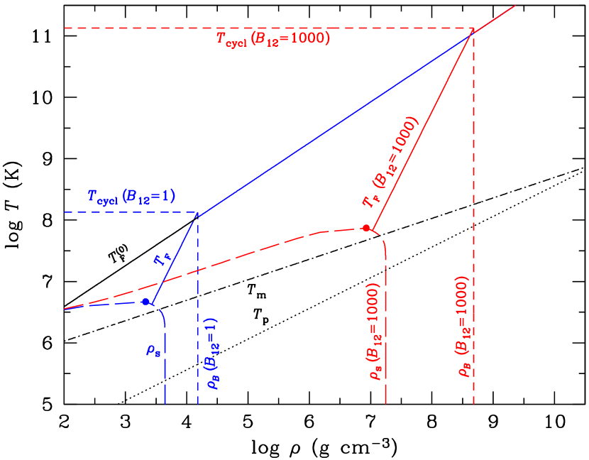
Figure 1: Characteristic density-temperature domains at $B=10^{12}$ G (blue online) and $10^{15}$ G (red online) for fully-ionized iron. Solid lines indicate the Fermi temperature as function of density, the dotted line shows the plasma temperature, the dot-dashed line shows the melting temperature as function of density, short and long dashes delimit the domains of strongly quantizing magnetic field and of magnetic condensation, respectively, and the heavy dots mark the critical point for the condensation (Sect. 7.3).

4.2.3 Strongly degenerate electrons

If the electrons are strongly degenerate, then one can apply the Sommerfeld expansion (Sect. 3.1) and obtain $F_{\mathrm{id}}^{\mathrm{(e)}}\approx F_{0}^{\mathrm{(e)}}+\Delta F$, where $F_{0}^{\mathrm{(e)}}=\epsilon_{\mathrm{F}}N_{\mathrm{e}}-P_{0}^{\mathrm{(e)}}V$ is the zero-temperature value and $\Delta F$ is a thermal correction. According to Eqs. 24 and 52, the zero-temperature pressure $P_{0}$ is

$$P_{0}^{\mathrm{(e)}}=\frac{P_{\mathrm{r}}\,b}{2\pi^{2}}\sum_{n=0}^{n_{\mathrm{max}}}\sum_{\sigma}(1+2bn)\,\mathcal{I}_{1/2}^{(0)}(\tilde{\epsilon}_{n}),$$ (57)

where $P_{\mathrm{r}}\equiv m_{\mathrm{e}}^{4}c^{5}/\hbar^{3}=1.4218\times 10^{25}\mathrm{\leavevmode\nobreak\ dyn\leavevmode\nobreak\ cm}^{-2}$ is the relativistic unit of pressure, $n_{\mathrm{max}}$ is the maximum integer $n$ for which $p_{n}^{2}(\epsilon)>0$, and $\tilde{\epsilon}_{n}\equiv\epsilon_{\mathrm{F}}/m_{\mathrm{e}}c^{2}+1-\sqrt{1+2bn}$. According to Eqs. 24 and 51, the Fermi energy $\epsilon_{\mathrm{F}}$ is determined by the condition

$$n_{\mathrm{e}}=\left(\frac{m_{\mathrm{e}}c}{\hbar}\right)^{3}\frac{b}{2\pi^{2}}\sum_{n=0}^{n_{\mathrm{max}}}\sum_{\sigma}\,(1+2bn)^{1/2}\mathcal{I}_{1/2}^{(1)}(\tilde{\epsilon}_{n}).$$ (58)

In order to obtain the chemical potential $\mu_{\mathrm{e}}=\epsilon_{\mathrm{F}}+\Delta\epsilon$ with fractional accuracy $\sim\chi_{\mathrm{e}}^{-2}$, we retain two terms in Eq. 24, insert it into Eq. 51, approximate $\mathcal{I}_{\nu}^{(n)}(\tilde{\mu}_{n})$ in the vicinity of $\tilde{\mu}_{n}=\epsilon_{n}$ by

$$\mathcal{I}_{\nu}^{(n)}(\tilde{\mu}_{n})\approx\mathcal{I}_{\nu}^{(n)}(\tilde{\epsilon}_{n})+\mathcal{I}_{\nu}^{(n+1)}(\tilde{\epsilon}_{n})\,\Delta\tilde{\epsilon},$$ (59)

where $\tilde{\mu}_{n}\equiv\chi_{n}\tau$ and $\Delta\tilde{\epsilon}\equiv\Delta\epsilon/m_{\mathrm{e}}c^{2}$, and drop the higher-order terms containing $(\tau^{2}\Delta\tilde{\epsilon})$. Then

$$\Delta\tilde{\epsilon}\approx-\frac{\pi^{2}\tau^{2}}{6}\frac{\sum_{n=0}^{n_{\mathrm{max}}}\sum_{\sigma}(1+2bn)^{-1/2}\mathcal{I}_{1/2}^{(3)}(\tilde{\epsilon}_{n})}{\sum_{n=0}^{n_{\mathrm{max}}}\sum_{\sigma}(1+2bn)^{1/2}\mathcal{I}_{1/2}^{(2)}(\tilde{\epsilon}_{n})}\,.$$ (60)

The thermal correction to the pressure equals

$$\Delta P=P_{\mathrm{r}}\,b\sum_{n=0}^{n_{\mathrm{max}}}\sum_{\sigma}(1+2bn)\left(\frac{\tau^{2}}{12}\,\mathcal{I}_{1/2}^{(2)}(\tilde{\epsilon}_{n})+\frac{\Delta\tilde{\epsilon}}{2\pi^{2}}\,\mathcal{I}_{1/2}^{(1)}(\tilde{\epsilon}_{n})\right)\,,$$ (61)

and the thermal correction to the free energy and internal energy

$$\Delta F=-\Delta U=N_{\mathrm{e}}\,\Delta\epsilon-V\Delta P.$$ (62)

The leading contribution to the heat capacity is $C_{V}^{\mathrm{(e)}}=2\Delta U/T$. As in the nonmagnetic case, $C_{V}^{\mathrm{(e)}}$ is proportional to $T$ at $T\to 0$, but with a different proportionality coefficient.

4.2.4 Strongly degenerate electrons in a strongly quantizing magnetic field

If the magnetic field is strongly quantizing and the electrons are strongly degenerate (which corresponds to the triangular domains in Fig. 1 defined by conditions $\rho<\rho_{B}$ and $T<T_{\mathrm{F}}$), then

$$F_{0}^{\mathrm{(e)}} = \left[(1+x_{B}^{2})^{1/2}-1\right]N_{\mathrm{e}}m_{\mathrm{e}}c^{2}-P_{0}^{\mathrm{(e)}}V,$$ (63)

$$P_{0}^{\mathrm{(e)}} = \frac{P_{\mathrm{r}}\,b}{(2\pi)^{2}}\,\left[x_{B}\,(1+x_{B}^{2})^{1/2}-\ln\left(x_{B}+(1+x_{B}^{2})^{1/2}\right)\right].$$ (64)

In the nonrelativistic ($x_{B}\ll 1$) and ultrarelativistic ($x_{B}\gg 1$) limits, we have $P_{0}^{\mathrm{(e)}}\simeq P_{\mathrm{r}}\,b\,x_{B}^{3}/6\pi^{2}\propto n_{\mathrm{e}}^{3}$ and $P_{0}^{\mathrm{(e)}}\simeq P_{\mathrm{r}}\,b\,x_{B}^{2}/4\pi^{2}\propto n_{\mathrm{e}}^{2}$, respectively. Compared with the nonmagnetic case (Papers I and II), the dependence $P_{0}^{\mathrm{(e)}}(n_{\mathrm{e}})$ is steeper, but $P$ is lower everywhere except for $n_{\mathrm{e}}\approx n_{B}$. Thus, a strongly quantizing magnetic field softens the EOS of degenerate electrons.

The thermal corrections (Eqs. 60 – 62) simplify to

$$\Delta\tilde{\epsilon}\approx-\frac{\pi^{2}\tau^{2}}{6(1+x_{B}^{2})^{1/2}x_{B}^{2}},$$ (65)

$$\Delta P=P_{\mathrm{r}}\,\frac{b\tau^{2}}{12}\,\frac{2+x_{B}^{2}}{(1+x_{B}^{2})^{1/2}\,x_{B}^{\phantom{2}}},$$ (66)

$$\frac{\Delta U}{V}=-\frac{\Delta F}{V}=P_{\mathrm{r}}\,\frac{b\tau^{2}}{12}\,\frac{(1+x_{B}^{2})^{1/2}}{x_{B}},$$ (67)

$$\frac{C_{V}^{\mathrm{(e)}}}{N_{\mathrm{e}}k_{\mathrm{B}}}=\frac{\pi^{2}\tau}{3}\,\frac{(1+x_{B}^{2})^{1/2}}{x_{B}^{2}}\,.$$ (68)

The last equation differs from the nonmagnetic case (Paper II) in that $x_{B}$ replaces $x_{\mathrm{r}}$ and $\pi^{2}/3$ replaces $\pi^{2}$.

4.2.5 Nonrelativistic limit

In the nonrelativistic limit ($p_{\mathrm{F}}\ll m_{\mathrm{e}}c$ and $T\ll T_{\mathrm{r}}$), Eqs. 51 and 52 simplify to

$$n_{\mathrm{e}}=\frac{1}{2\pi^{3/2}a_{\mathrm{m}}^{2}\lambda_{\mathrm{e}}}\sum_{n,\sigma}I_{-1/2}(\chi_{n}),\leavevmode\nobreak\ \leavevmode\nobreak\ P_{\mathrm{e}}=\frac{k_{\mathrm{B}}T}{\pi^{3/2}a_{\mathrm{m}}^{2}\lambda_{\mathrm{e}}}\sum_{n,\sigma}I_{1/2}(\chi_{n}).$$ (69)

In the nondegenerate regime ($T\gg T_{\mathrm{F}}$), one has $I_{\nu}(\chi)\approx\mathrm{e}^{\chi}\,\Gamma(\nu+1)$, where $\Gamma(\nu+1)$ is the gamma-function. Then Eq. 69 yields $P_{\mathrm{id}}^{\mathrm{e}}=n_{\mathrm{e}}k_{\mathrm{B}}T$ and

$$\chi_{\mathrm{e}}=\ln(n_{\mathrm{e}}\lambda_{\mathrm{e}}^{3}/2)-\ln(\zeta/4)+\ln[\tanh(\zeta/4)]$$ (70)

which provides the free energy $F_{\mathrm{id}}^{(e)}=(\chi_{\mathrm{e}}-1)\,N_{\mathrm{e}}k_{\mathrm{B}}T$.

As follows from Eq. 70, the reduced internal energy $U_{\mathrm{id}}^{\mathrm{e}}/N_{\mathrm{i}}k_{\mathrm{B}}T$ and heat capacity $C_{V,\mathrm{id}}^{\mathrm{e}}/N_{\mathrm{i}}k_{\mathrm{B}}$ of the Boltzmann gas decrease with increasing $\zeta$. In a strongly quantizing magnetic field ($\zeta\gg 1$), they tend to $1/2$ instead of $3/2$ because the gas becomes effectively one-dimensional. The only kinetic degree is along the magnetic field.

In the nonquantizing field ($\zeta\ll 1$), the two last terms in Eq. 70 cancel out, so that the standard expression $F_{\mathrm{id}}^{(e)}=N_{\mathrm{e}}k_{\mathrm{B}}T\,[\ln(n_{\mathrm{e}}\lambda_{\mathrm{e}}^{3}/2)-1]$ is recovered. In the strongly quantizing, nondegenerate regime ($\rho<\rho_{B}$ and $T_{\mathrm{F}}\ll T\ll T_{\mathrm{cycl}}$), the last term of Eq. 70 vanishes, which yields

$$F_{\mathrm{id}}^{(e)}=N_{\mathrm{e}}k_{\mathrm{B}}T\left[\ln(2\pi a_{\mathrm{m}}^{2}\lambda_{\mathrm{e}}n_{\mathrm{e}})-1\right].$$ (71)

4.3 Thermodynamic and kinetic pressures

The above expressions for pressure of a magnetized gas of charged particles are based on the principles of thermodynamics (Landau & Lifshitz 1980), according to which $P=-(\partial F/\partial V)_{T,B}$. Alternatively, the pressure can be calculated from the microscopic dynamics as the sum of the changes of kinetic momenta of all particles reflected off a unit surface per unit time. The result of the latter calculation, the kinetic pressure $P^{\mathrm{kin}}$, depends on the orientation of the surface relative to $\bm{B}$ (Canuto & Chiu 1968). If the surface is perpendicular to $\bm{B}$, then one gets the kinetic pressure $P_{\|}^{\mathrm{kin}}=P$, which acts along the field lines, the longitudinal pressure. If the surface is parallel to the field, one gets a different (transverse) kinetic pressure, which can be expressed (Blandford & Hernquist 1982) as

$$P_{\perp}^{\mathrm{kin}}=-\Omega/V+B\,(\partial\Omega/\partial B)_{V,T}=P-MB,$$ (72)

where $M=-\partial\Omega/\partial B$ is the magnetization.

In order to resolve the apparent paradox, one should take the magnetization current density $\bm{j}_{\mathrm{m}}=c\,\nabla\times{\bm{M}}$ into account; when boundaries are present, this volume current should be supplemented by the surface current $c\bm{M}\times\bm{B}/B$ (see, e.g., Griffith 1999). As argued by Blandford & Hernquist (1982), if we compress the electron gas perpendicular to $\bm{B}$ then we must do work against the Lorentz force density $\bm{j}_{\mathrm{m}}\times\bm{B}/c$, which gives an additional contribution to the total transverse pressure and makes it equal to $P$. Because this point still causes confusion in some publications, let us illustrate it with a simple example.

If the pressure were anisotropic, then one might expect an anisotropic density gradient in a strongly magnetized star. Let us consider a small volume element in the star, assuming that we can treat $\bm{B}$, $T$, and gravitational acceleration $\bm{g}$ as constants within this volume, and $z$ axis is directed along $\bm{g}$. Hydrostatic equilibrium implies that the density of gravitational force, $\rho\bm{g}$, is balanced by the density of forces created by plasma particles. The crucial point is that the magnetization contributes to this balance.

Let us compare the cases where $\bm{B}$ is parallel and perpendicular to $\bm{g}$. In the first case, the $z$-component of the Lorentz force is absent, and we get the standard equation of hydrostatic equilibrium: $\rho g=\mathrm{d}P_{\|}^{\mathrm{kin}}/\mathrm{d}z=\mathrm{d}P/\mathrm{d}z$. In the second case, the gradients of the kinetic pressure $\mathrm{d}P_{\perp}^{\mathrm{kin}}/\mathrm{d}z$ and of the Lorentz force density $B\,\mathrm{d}M/\mathrm{d}z$ act in parallel. In the constant and uniform magnetic field, $\mathrm{d}M/\mathrm{d}z$ is not zero, but is related to the density gradient:

$$\frac{\mathrm{d}M}{\mathrm{d}z}=\frac{\partial M(\rho,T,B)}{\partial\rho}\,\frac{\mathrm{d}\rho}{\mathrm{d}z}=-\frac{\partial^{2}\Omega(\rho,T,B)}{V\partial\rho\,\partial B}\,\frac{\mathrm{d}\rho}{\mathrm{d}z}.$$ (73)

Then the equilibrium condition takes the form $\rho g={\mathrm{d}P_{\perp}^{\mathrm{kin}}}/{\mathrm{d}z}+B\,{\mathrm{d}M}/{\mathrm{d}z}={\mathrm{d}P}/{\mathrm{d}z},$ which is the same as in the first case. Furthermore, one can express $P$ through $\rho$ using some EOS. In the considered example, $\mathrm{d}P/\mathrm{d}z=[\partial P(\rho,T,B)/\partial\rho]\,\mathrm{d}\rho/\mathrm{d}z$, so that $\mathrm{d}\rho/\mathrm{d}z$ is also the same in both cases. Thus, the stellar hydrostatic profile is determined by the isotropic thermodynamic pressure $P$, which automatically includes magnetization.

5 Magnetic effects on the EOS of a Coulomb liquid

5.1 Electron exchange and correlation

The effects of a magnetic field on the contribution to the free energy due to electron exchange and correlation were studied either in the regime of strong degeneracy and strongly quantizing magnetic fields (Danz & Glasser 1971; Banerjee et al. 1974; Fushiki et al. 1989; see also Morbec & Capelle 2008 for an instructive discussion of the previous results and the inclusion of the second Landau level contribution), or at low densities (Alastuey & Jancovici 1980; Cornu 1998; Steinberg et al. 1998, 2000). In a previous work (Potekhin et al. 1999) we suggested a modification of the field-free expression for $F_{\mathrm{ee}}$, which matches available exact limiting expressions, including the cases of nonquantizing, strongly quantizing degenerate, and strongly quantizing nondegenerate plasmas. The modification consists in replacing $F_{\mathrm{ee}}(\theta,\Gamma_{\mathrm{e}})$ by $F_{\mathrm{ee}}(\theta^{\ast},\Gamma_{\mathrm{e}})$, where

$$\theta^{\ast}=\frac{\theta_{0}+\theta_{B}}{\displaystyle 1+\frac{\theta_{B}}{\theta_{0}}\,\exp(-\theta_{B}^{-1})\,\frac{\cosh(\zeta/2)}{[\cosh(\zeta/4)]^{2}}\,\frac{\tanh(\zeta/4)}{\zeta/4}\,\frac{\mathrm{arctanh}\,\xi}{\xi}}\,,$$ (74)

$\xi=[1-(4/\zeta)\tanh(\zeta/4)]^{1/2}$, and $\theta_{0}$ and $\theta_{B}$ are given by Eqs. 2 and 56, respectively, at fixed $n_{\mathrm{e}}$ and $T$.

5.2 Wigner-Kirkwood term

For the same reason as in Sect. 3.2.1, the treatment of the quantum effects in the ion liquid is restricted by the Wigner-Kirkwood term. Its expression in an arbitrary magnetic field was obtained by Alastuey & Jancovici (1980):

$$f_{\mathrm{ii}}^{(2)}=\frac{\eta^{2}}{24}\,\left[\frac{4}{\zeta_{\mathrm{i}}\,\tanh(\zeta_{\mathrm{i}}/2)}-\frac{8}{\zeta_{\mathrm{i}}^{2}}+\frac{1}{3}\right].$$ (75)

The function in the square brackets monotonously varies from 1 at $\zeta_{\mathrm{i}}\to 0$ to $1/3$ at $\zeta_{\mathrm{i}}\to\infty$, reflecting the effective reduction of the degrees of freedom of the classical ion motion from $d=3$ at $B=0$ to $d=1$ for a strongly quantizing field. At small $\zeta_{\mathrm{i}}$, $f_{\mathrm{ii}}^{(2)}\approx(\eta^{2}/24)\,(1-\zeta_{\mathrm{i}}^{2}/90)$.

5.3 Electron-ion correlations

Using the linear response theory in the Thomas-Fermi limit, Fushiki et al. (1989) evaluated the electron polarization energy for a dense plasma in a strongly quantizing magnetic field at zero temperature, assuming that the ions remain classical (unaffected by the field). A comparison with the analogous zero-field result shows that the strongly quantizing magnetic field ($\gamma_{\mathrm{m}}r_{\mathrm{s}}^{2}>2.23$) increases the polarization energy at high densities ($r_{\mathrm{s}}\ll 1$) by a factor of $0.8846\,\gamma_{\mathrm{m}}^{2}r_{\mathrm{s}}^{4}$ (Potekhin et al. 1999).

Recently, Sharma & Reddy (2011) calculated the screening of the ion-ion potential due to electrons in a large magnetic field $B$ at $T=0$, using the one-loop representation of the polarization function. Their results for the strongly quantizing magnetic field show that the screening is anisotropic, and the screened ion potential exhibits Friedel oscillations with period $\pi\hbar/p_{\mathrm{F}}$ in a cylinder of a radius $\sim\pi\hbar/p_{\mathrm{F}}$ along the magnetic field line that passes through the Coulomb center. Sharma & Reddy suggest that this long-range oscillatory behavior can affect the ion lattice structure. However, finite temperature should damp these oscillations, so that they are pronounced only at $T\ll T_{\mathrm{F}}$, i.e., deep within the triangular domains formed by the lines $T_{\mathrm{F}}$ and $\rho_{B}$ in Fig. 1. At the typical pulsar magnetic fields $B\sim 10^{12}$ G, this requires an unusually low temperature of the neutron-star crust. On the other hand, the conditions $T\ll T_{\mathrm{F}}$ and $\rho<\rho_{B}$ can be easily fulfilled in the outer crust of magnetars at $B\sim 10^{15}$ G (cf. Fig. 1 and the top panel of Fig. 8), but in this case the Friedel oscillations are strongly suppressed because the electrons are ultrarelativistic.

To the best of our knowledge, the magnetic effects on the electron polarization energy have not been calculated at finite temperatures or in the case where the field is not strongly quantizing. In view of the limited scope and limited applicability of the available results on the magnetic effects, we use the nonmagnetic expression for $F_{\mathrm{ie}}$ in our code (Appendix C).

6 Harmonic Coulomb crystals in the magnetic field

The magnetic effects on Coulomb crystals have been studied only in the harmonic approximation. Nagai & Fukuyama (1982, 1983) calculated phonon spectra of body-centered cubic (bcc), face-centered cubic (fcc), and hexagonal closely-packed (hcp) OCP lattices. They compared the energies of zero-point vibrations at different values of parameters $\beta$ and $R_{\mathrm{S}}$ and found conditions of stability of every lattice type. However, Baiko (2000, 2009) noticed that their choice of the magnetic-field direction did not provide the minimum of the total energy.

Usov et al. (1980) obtained the equations for oscillation modes of a harmonic OCP crystal and studied its phonon spectrum in a quantizing magnetic field in several limiting cases. These authors discovered a “soft” phonon mode with dispersion relation $\omega_{\bm{k}\alpha}\propto k^{2}$ near the center of the Brillouin zone, which leads to the unusual dependence of the heat capacity of the lattice $C_{V,\mathrm{lat}}\propto T^{3/2}$ at $T\to 0$ instead of the Debye law $C_{V,\mathrm{lat}}\propto T^{3}$. Usov et al. (1980) argued that a strong magnetic field should increase stability of the crystal.

Baiko (2000, 2009) studied the magnetic effects on the phonon spectrum of the harmonic Coulomb crystals and calculated its energy, entropy, and heat capacity. We have found that his results can be approximately reproduced by the analytical expressions presented below.

6.1 Thermal phonon contributions

Figure 2: Thermal phonon contribution to the reduced internal energy $u_{\mathrm{th}}=U_{\mathrm{th}}/N_{\mathrm{i}}k_{\mathrm{B}}T$ as a function of $\log(T/T_{\mathrm{p}})=-\log\eta$ at $\beta=\hbar\omega_{\mathrm{ci}}/k_{\mathrm{B}}T_{\mathrm{p}}=0$, 1, 10, 100, and $10^{3}$ (numbers near the lines). The analytical approximation in Eq. 76 (dotted lines) and in Eq. 78 (short-dashed lines) are compared with the numerical results of Baiko (2009) (solid lines for $\beta=1$, 10, and 100).

Without a magnetic field, the thermal phonon contribution $f_{\mathrm{th}}$ to the reduced free energy of a Coulomb crystal $F/N_{\mathrm{i}}k_{\mathrm{B}}T$ is a function of a single argument $\eta$, described by a simple analytical expression (Baiko et al. 2001). The magnetic field introduces the second independent dimensionless argument $\beta$. The functional dependence of thermodynamic functions on $\eta$ and $\beta$ is not simple. Baiko (2009) identified five characteristic sectors of the $\eta$ – $\beta$ plane:
   1.  $\eta<1$ and $\beta<\eta^{-1}$ – weakly magnetized classical crystal,
   2.  $\eta>1$ and $\beta<\eta^{-1}$ – weakly magnetized quantum crystal,
   3.  $\eta<1$ and $\beta>\eta^{-1}$ – strongly magnetized classical crystal,
   4.  $\eta>\beta>\eta^{-1}$ – strongly magnetized quantum crystal,
   5.  $\beta>\eta>1$ – very strongly magnetized quantum crystal.
Note that the condition $\beta>\eta^{-1}$ is equivalent to $\zeta_{\mathrm{i}}>1$. Thus, the magnetic field strongly affects the thermodynamic functions of a Coulomb crystal when $\hbar\omega_{\mathrm{ci}}>k_{\mathrm{B}}T$, that is the same condition as for the gas and liquid phases.

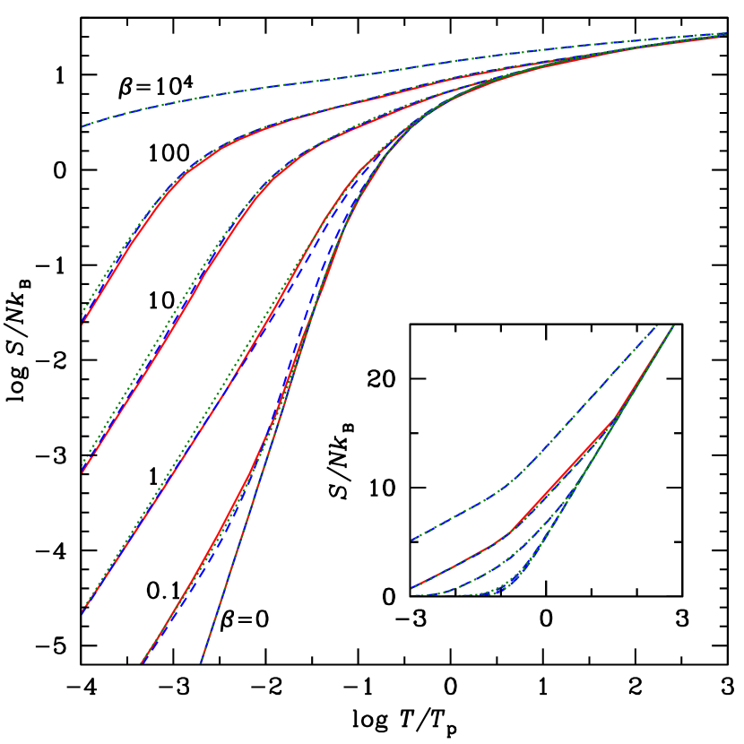
Figure 3: Thermal phonon contribution to the reduced entropy $s_{\mathrm{th}}=S_{\mathrm{th}}/N_{\mathrm{i}}k_{\mathrm{B}}T$ as a function of $\log(T/T_{\mathrm{p}})$ at $\beta=\hbar\omega_{\mathrm{ci}}/k_{\mathrm{B}}T_{\mathrm{p}}=0$, 0.1, 1, 10, 100, and $10^{4}$ (numbers near the lines). The analytical approximations in Eq. 77 (dotted lines) and in Eq. 79 (dashed lines) are compared with the numerical results of Baiko (2009) (solid lines for $\beta\leqslant 100$). The inset shows the same approximations in the linear scale for $s_{\mathrm{th}}$; here, the solid line corresponds to the numerical data at $\beta=100$.

For astrophysical applications, we have constructed an analytical representation of the EOS of the magnetized Coulomb crystal, which is asymptotically exact in each of the five sectors far from their boundaries, exactly recovers the nonmagnetic fit of Baiko et al. (2001) in the limit $\beta\to 0$, and reaches a reasonable compromise between simplicity and accuracy.

The term $f_{\mathrm{th}}$ in Eq. 32 can be rewritten as $f_{\mathrm{th}}=u_{\mathrm{th}}-s_{\mathrm{th}},$ where $u_{\mathrm{th}}=U_{\mathrm{th}}/N_{\mathrm{i}}k_{\mathrm{B}}T$ and $s_{\mathrm{th}}=S_{\mathrm{th}}/N_{\mathrm{i}}k_{\mathrm{B}}$ are the thermal contributions to the reduced internal energy and entropy. We approximately represent $u_{\mathrm{th}}$ by the function

$$\tilde{u}=\frac{u_{\mathrm{th}}^{(0)}}{1+0.5\left[1+(3/\zeta_{\mathrm{i}})^{5/2}\right]^{-2/5}}+\frac{\psi\,/\sqrt{1+24/\eta^{2}}}{1+15\,\beta/\eta+\psi},$$ (76)

where $\psi=12.5\,(\beta/\eta)^{3/2}+119\,(\beta/\eta)^{2}$ and $\zeta_{\mathrm{i}}=\beta\eta$, and we represent $s_{\mathrm{th}}$ by the function

$$\tilde{s}=s_{\mathrm{th}}^{(0)}+\ln\left(1+\frac{20.8\,(\beta/\eta)^{3/2}+122.5\,(\beta/\eta)^{2}}{(1+7.9\,\beta/\eta)\,(1+42/\eta^{2})\,(1+\zeta_{\mathrm{i}}^{-1})^{4}}\right).$$ (77)

In these equations, $u_{\mathrm{th}}^{(0)}$ and $s_{\mathrm{th}}^{(0)}$ are the values of $u_{\mathrm{th}}$ and $s_{\mathrm{th}}$ at $\beta=0$. Equations (76) and (77) exactly reproduce the known asymptotic limits: $u_{\mathrm{th}}=3$ in the classical nonmagnetic limit ($\eta\ll\beta\ll 1$), $u_{\mathrm{th}}=2$ in the classical magnetic limit ($\eta\ll\beta^{-1}\ll 1$), $u_{\mathrm{th}}=1$ in the case where $\beta\gg\eta\gg 1$, and $u_{\mathrm{th}}=0.6s_{\mathrm{th}}\propto\eta^{-3/2}$, if $\eta\to\infty$ at $\beta={}$constant.

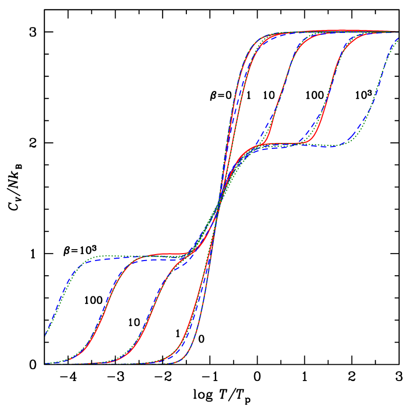
Figure 4: Thermal phonon contribution to the reduced heat capacity $C_{V,\mathrm{lat}}/N_{\mathrm{i}}k_{\mathrm{B}}T$ as a function of $\log(T/T_{\mathrm{p}})$ at $\beta=\hbar\omega_{\mathrm{ci}}/k_{\mathrm{B}}T_{\mathrm{p}}=0$, 1, 10, 100, and $10^{3}$ (numbers near the lines). The analytical approximation in Eq. 80) (short-dashed lines) is compared with the numerical results of Baiko (2009) (solid lines for $\beta=0$, 1, 10, and 100). The dotted lines correspond to the first term on the r.h.s. of Eq. 80.

The functions $\tilde{u}(\eta,\beta)$ and $\tilde{s}(\eta,\beta)$ are displayed in Figs. 2 and 3. Their accuracy is seen from a comparison with the numerical results (Baiko 2009), also shown in the figures. However, if the complete consistency of different thermodynamic functions is required, Eqs. (76) and (77) should not be used directly, but should be first combined into $f_{\mathrm{th}}=\tilde{u}-\tilde{s}.$ Then one can calculate thermodynamic functions by differentiating the function $f_{\mathrm{th}}(\eta,\beta)$. In this way we obtain, for example,

$$u_{\mathrm{th}}=\frac{U_{\mathrm{th}}}{N_{\mathrm{i}}k_{\mathrm{B}}T}=\tilde{u}+\Delta u,$$ (78)

$$s_{\mathrm{th}}={S_{\mathrm{th}}}/{N_{\mathrm{i}}k_{\mathrm{B}}}=\tilde{s}+\Delta u,$$ (79)

$$\frac{C_{V,\mathrm{th}}}{N_{\mathrm{i}}k_{\mathrm{B}}}=-\left(\frac{\partial\tilde{s}}{\partial\ln\eta}\right)_{\beta}-\left(\frac{\partial\Delta u}{\partial\ln\eta}\right)_{\beta},$$ (80)

$$\mbox{where\leavevmode\nobreak\ \leavevmode\nobreak\ }\Delta u=\left(\frac{\partial\tilde{s}}{\partial\ln\eta}\right)_{\beta}-\left(\frac{\partial\tilde{u}}{\partial\ln\eta}\right)_{\beta}-\tilde{u}.$$ (81)

Note that the relation between the phonon contributions to pressure and internal energy, $2P_{\mathrm{th}}V=U_{\mathrm{th}}$, which is standard for a nonmagnetized harmonic crystal, is invalid in the strongly magnetized crystal because both dimensionless arguments $\eta$ and $\beta$ depend on density.

Approximations in Eqs. 78) – 80 are shown in Figs. 2 – 4. Their reasonable behavior beyond the range of available numerical data is demonstrated by plotting them also at larger $\beta=10^{3}$ and $10^{4}$.

6.2 Zero-point vibrations

Because motions of the ions are confined by the magnetic field in the transverse direction, they exhibit quantum oscillations in the ground state (Landau 1930; Landau & Lifshitz 1977). The energy of these oscillations is $\hbar\omega_{\mathrm{ci}}/2$ for every ion, which gives the term $\zeta_{\mathrm{i}}/2$ in Eq. 42. In a Coulomb crystal, the motion of an ion is confined in an effective potential well, centered at its equilibrium lattice site. The total energy of the zero-point quantum lattice oscillations $U_{\mathrm{q}}$ is given by Eq. 30.

In the case where the crystal is placed in a magnetic field, $U_{\mathrm{q}}$ includes contributions due to both magnetic and lattice confinements of the ion motion. However, since the magnetic contribution $N_{\mathrm{i}}\hbar\omega_{\mathrm{ci}}/2$ is common in all phase states, we take it as the zero energy point in our code and separate it from the lattice contribution that is specific to the solid phase. Then Eq. 30 becomes

$$U_{\mathrm{q}}=\frac{3}{2}N_{\mathrm{i}}\hbar\omega_{\mathrm{p}}u^{\prime}_{1}+\frac{1}{2}N_{\mathrm{i}}\hbar\omega_{\mathrm{ci}},$$ (82)

and in Eq. 32 we have $1.5u_{1}\eta=1.5u^{\prime}_{1}\eta+\zeta_{\mathrm{i}}/2$, where we have defined

$$u^{\prime}_{1}=u_{1}-\beta/3.$$ (83)

The reduced frequency moment $u^{\prime}_{1}$ still depends on $\beta$, because the character of ion vibrations is affected by the magnetic field (they become essentially one-dimensional if $B$ is extremely large), but the latter dependence is relatively weak. Having extracted $u^{\prime}_{1}$ from the available numerical results for $u_{1}$ (Baiko 2009; Baiko & Yakovlev 2012), we can represent it by the simple interpolation

$$u^{\prime}_{1}(\beta)=\frac{u_{1}^{0}+1.27\beta^{9/8}u_{1}^{\infty}}{1+1.27\beta^{9/8}},$$ (84)

where $u_{1}^{0}$ is the zero-field value and $u_{1}^{\infty}$ is the limit of $u^{\prime}_{1}(\beta)$ at $\beta\to\infty$. Only one of the three phonon branches contributes to $u^{\prime}_{1}$ in the latter limit, therefore $u_{1}^{\infty}\sim u_{1}^{0}/3$. For the bcc crystal, $u_{1}^{0}=0.5113875$, whereas $u_{1}^{\infty}$ varies between 0.18 and 0.19 depending on the orientation of the lattice in the magnetic field. In Fig. 5 we show $u^{\prime}_{1}$ and the logarithm (base 10) of $u_{1}$ versus $\beta$.

Figure 5: Reduced first moment of phonon frequencies $u^{\prime}_{1}$ (solid line) and $\log u_{1}$ (dashed line) as functions of $\beta=\hbar\omega_{\mathrm{ci}}/T_{\mathrm{p}}$. The dotted line shows the asymptote $\log(\beta/3)$.

Usov et al. (1980) noticed that the energy of a crystal depends on its orientation in a strong magnetic field. However, numerical calculations (Baiko 2000, 2009) show that this dependence is very weak. For example, the difference $\Delta u_{1}$ between the values of $u_{1}$ for two orientations, where the field lines connect an ion with its nearest neighbor in the first case and with a next-order nearest neighbor in the second case, is approximately

$$\Delta u_{1}=\frac{\,\beta^{15/4}}{(1+\beta^{3/2})^{5/2}}\,(\Delta u_{1})_{\mathrm{max}}$$ (85)

with saturation level $(\Delta u_{1})_{\mathrm{max}}=0.0064$ for the bcc lattice.

6.3 Comparison with the Baiko-Yakovlev fit

After the present work was completed, we became aware of an independent study by Baiko & Yakovlev (2012), who developed another set of approximations for the free energy of the harmonic Coulomb crystal in a magnetic field. They presented the free energy as a sum of three terms corresponding to the contributions from each of the three phonon modes in the bcc crystal. Thus each of these terms has a clear physics meaning, while our fitting expressions give only the total contribution, which cannot be easily decomposed to three parts corresponding to the separate phonon modes.

Unlike our fit, the fit of Baiko & Yakovlev (2012) does not exactly reproduce the very accurate results of Baiko et al. (2001) in the limit $\beta\to 0$. At finite $\beta$, both sets of fitting expressions accurately reproduce the asymptotes at $T\ll T_{\mathrm{p}}$ and $T\gg T_{\mathrm{p}}$ and have similar accuracies within several percent points in the intermediate range $0.1T_{\mathrm{p}}/\beta\lesssim T\lesssim 10T_{\mathrm{p}}$. Meanwhile, our approximation is simpler: the Baiko-Yakovlev approximation contains 27 independent numerical fitting parameters, whereas our fits 76 and 77 contain together only 9 such parameters.

7 Examples and discussion

7.1 Thermodynamic functions

Characteristic features of the EOS can be seen in Fig. 6. Here, we have chosen the plasma parameters that are typical for outer envelopes of isolated neutron stars: we consider fully-ionized iron ($Z=26$, $A=56$) at $T=10^{7}$ K and $B=10^{12}$ G (for illustration, the density range is extended to $\rho\lesssim 10^{5}$ neglecting the bound states that can be important in this $\rho$ – $T$ domain). We plot the normalized pressure $p=P/n_{\mathrm{i}}k_{\mathrm{B}}T$, entropy $S/N_{\mathrm{i}}k_{\mathrm{B}}$, heat capacity $c_{V}=C_{V}/N_{\mathrm{i}}k_{\mathrm{B}}$, and logarithmic derivatives of pressure $\chi_{\rho}$ and $\chi_{T}$ as functions of density. Dashed lines show these functions in the absence of quantizing magnetic field. The vertical dotted lines marked by numbers separate different characteristic domains, consecutively entered with increasing density: onset of electron degeneracy at $B=0$ ($T_{\mathrm{F}}^{\mathrm{(0)}}=T$) and at $B=10^{12}$ G ($T_{\mathrm{F}}=T$), population of excited Landau levels ($\rho=\rho_{B}$), melting point with formation of a classical Coulomb crystal ($T_{\mathrm{m}}=T$), and quantum effects in the crystal ($T_{\mathrm{p}}=T$).

At low densities, the ideal-gas values are approached: $p=1+Z$, $\chi_{\rho}=\chi_{T}=1$, $c_{V}=(3+3Z)/2$ at $B=0$, and $c_{V}=(3+Z)/2$ at $B=10^{12}$ G. The latter difference is because at $\rho<\rho_{B}$ the electron gas is effectively one-dimensional due to the strong magnetic quantization.

With increasing density, the reduced pressure $p$ first decreases below its ideal-gas value due to the Coulomb nonideality and then increases due to the electron degeneracy. The increase occurs earlier at zero field than in the strong magnetic field, because of the delayed onset of the degeneracy (Sec. 4). When $\rho>\rho_{B}\approx 1.5\times 10^{4}$ g cm^-3, the thermodynamic functions approach their zero-field values. The gradually decreasing oscillations correspond to consecutive filling of the electron Landau levels. The magnetic field $B=10^{12}$ G does not affect the ion contributions in Fig. 6, because it is nonquantizing for the iron nuclei at $T=10^{7}$ K ($\zeta_{\mathrm{i}}=0.00342$).

The liquid-solid phase transition occurs in Fig. 6 at $\rho\approx 8.25\times 10^{4}$ g cm^-3, where we adopt the classical OCP melting condition $\Gamma=175.2$ (Paper I). With further increase in density ($\rho\gtrsim 10^{6}$) the degeneracy becomes so strong that the energy and pressure are nearly independent of $T$ and $\chi_{T}$ strongly decreases. The normalized heat capacity gradually tends to its value $c_{V}=3$ characteristic of the classical simple crystal. At still higher density the ion motions become quantized ($T_{\mathrm{p}}\gg T$) which leads to the further decrease in the heat capacity and the entropy.

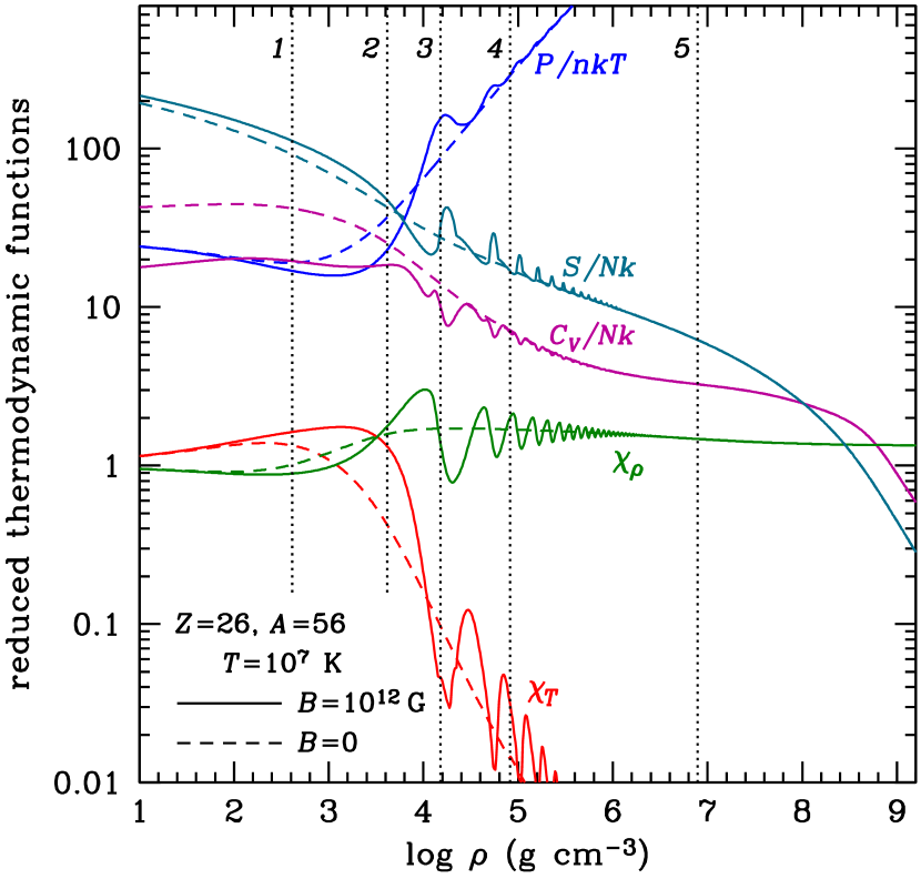
Figure 6: Reduced thermodynamic functions $P/n_{\mathrm{i}}k_{\mathrm{B}}T$, $S/N_{\mathrm{i}}k_{\mathrm{B}}$, $C_{V}/N_{\mathrm{i}}k_{\mathrm{B}}$, $\chi_{\rho}$, and $\chi_{T}$ for a fully-ionized nonmagnetic (dashed lines) and magnetized ($B=10^{12}$ G, solid lines) iron plasma at $T=10^{7}$ K. The vertical dotted lines mark the densities at which (1) $T_{\mathrm{F}}^{(0)}=T$, (2) $T_{\mathrm{F}}=T$, (3) $\rho=\rho_{B}$, (4) $\Gamma=\Gamma_{\mathrm{m}}$, and (5) $T_{\mathrm{p}}=T$.

Figure 7: Characteristics of the melting transition of nonideal carbon and iron plasmas at different field strengths $B$ (marked near the curves). Lower panel: the value $\Gamma_{\mathrm{m}}$ of the Coulomb coupling parameter $\Gamma$ at the melting point as function of mass density $\rho$. Upper panel: normalized latent heat per ion at the melting transition. The dot-dashed and dashed segments of the curves correspond to the domains of nonperturbative quantum effects ($T<0.5\,T_{\mathrm{p}}$) and electron response ($Z^{2}\,\textrm{Ry}>0.1\,\epsilon_{\mathrm{F}}$), respectively. The dotted horizontal lines mark the OCP values. The filled and open circles mark the positions of the real and virtual condensed surfaces (see text in Sect. 7.3).

7.2 Melting

The electron polarization, ion quantum effects, and quantizing magnetic field can shift the melting temperature. The lower panel of Fig. 7 shows the Coulomb coupling parameter $\Gamma$ at the melting (that is, the value $\Gamma_{\mathrm{m}}$ at which the free energies of the two phases are equal to each other); the upper panel displays the difference between the internal energies in the liquid and solid phases at the melting point (the latent heat $Q_{\mathrm{m}}=U_{\mathrm{liq}}-U_{\mathrm{sol}}$), divided by $N_{\mathrm{i}}k_{\mathrm{B}}T$. We plot the data for fully ionized ¹²C and ⁵⁶Fe at $B=0$ and $10^{13}$ G for carbon, $B=0$, $10^{14}$ G, and $10^{15}$ G for iron. The density range shown in the figure is typical for the outer envelopes of a neutron star and is also relevant for white dwarfs.

The position of the melting point is very sensitive to the accuracy of the free energies of the Coulomb liquid and crystal (see, e.g., Paper I). The polarization and quantum corrections to the classical OCP free energy are not known sufficiently well for finding the position of the melting point in the whole interval of densities shown in Fig. 7. The dot-dashed curves in this figure correspond to the domain where $T<0.5\,T_{\mathrm{p}}$. Here, the perturbation theory for the quantum effects in the liquid phase becomes progressively inaccurate. The dashed curves correspond to the domain where the binding energy of the hydrogen-like ion exceeds 10% of the Fermi energy, $Z^{2}\,\textrm{Ry}>0.1\,\epsilon_{\mathrm{F}}$, which corresponds to $a_{\mathrm{e}}\gtrsim 0.6a_{0}/Z$. Here, the perturbation treatment of the electron polarization in the crystal starts to be inaccurate. In addition, the position of the melting point cannot be traced to $\Gamma\lesssim 100$ – 120, because the available results for the anharmonic corrections to the free energy of a Coulomb crystal (Appendix B.2) are accurate only at larger $\Gamma$. Nevertheless, we can evaluate $\Gamma_{\mathrm{m}}$ in a certain interval of densities for each type of ions (the solid segments of the curves in the figure).

The values of $Q_{\mathrm{m}}$ in Fig. 7 roughly (within a factor of two) agree with the OCP value $Q_{\mathrm{m}}^{\mathrm{OCP}}=0.746N_{\mathrm{i}}k_{\mathrm{B}}T$ at $\Gamma_{\mathrm{m}}=175.2$ and with the values used in theoretical models of white dwarf cooling (e.g., Hansen 2004 and references therein). Most of the neutron star cooling models currently ignore the release of the latent heat at the crystallization of the neutron star envelopes (e.g., Yakovlev & Pethick 2004, and references therein).

Figure 7 shows that the strong magnetic fields tend to decrease $\Gamma_{\mathrm{m}}$ and thus stabilize the Coulomb crystal, in qualitative agreement with previous conjectures (Ruderman 1971; Kaplan & Glasser 1972; Usov et al. 1980; Lai 2001). At densities $\rho\sim 10^{7}$ – $10^{8}$ g cm^-3 corresponding to the “sensitivity strip” in the neutron-star cooling theory (Yakovlev & Pethick 2004), the stabilization proves to be significant at the magnetar field strengths $B=10^{14}$ – $10^{15}$ G. The results for ⁵⁶Fe in this $B$ interval, shown in the lower panel of Fig. 7, can be roughly (within 10%) described by the formula $\Gamma_{\mathrm{m}}(B)\approx\Gamma_{\mathrm{m}}(0)/(1+0.2\,\beta)$. At the typical pulsar field strengths, $B=10^{12}$ – $10^{13}$ G, the effect is noticeable at lower densities. However, these conclusions remain preliminary in the absence of an evaluation of the magnetic-field effects on the anharmonic corrections. In view of the limited applicability and incompleteness of the evaluation of $\Gamma_{\mathrm{m}}$ with account of the quantum, polarization, and magnetic effects, in applications we use the classical OCP value $\Gamma_{\mathrm{m}}=175.2$ as the fiducial melting criterion.

7.3 Magnetic condensation

Ruderman (1971) suggested that the strong magnetic field may stabilize molecular chains (polymers) aligned with the magnetic field and eventually turn the surface of a neutron star into the metallic solid state. Later studies have provided support for this conjecture, although the critical temperature $T_{\mathrm{crit}}$, below which this condensation occurs, remains very uncertain. Condensed surface density $\rho_{\mathrm{s}}$ is usually estimated as

$$\rho_{\mathrm{s},\xi}=561\,\xi\,AZ^{-0.6}\,B_{12}^{1.2}\textrm{\leavevmode\nobreak\ \leavevmode\nobreak\ \leavevmode\nobreak\ \mbox{g\leavevmode\nobreak\ cm${}^{-3}$}},$$ (86)

where $\xi\sim 1$ is an unknown numerical factor, which absorbs the theoretical uncertainty (Lai 2001; Medin & Lai 2006). The value $\xi=1$ corresponds to the EOS provided by the ion-sphere model (Salpeter 1961), which is close to the uniform model of Fushiki et al. (1989). For comparison, the results of the zero-temperature Thomas-Fermi model for ⁵⁶Fe at $10^{10}\mbox{\leavevmode\nobreak\ G}\leqslant B\leqslant 10^{13}$ G (Rögnvaldsson et al. 1993) can be approximated (within 4%) by $\rho_{\mathrm{s},\xi}$ with $\xi\approx 0.2+0.01/B_{12}^{0.56}$, whereas the finite-temperature Thomas-Fermi model of Thorolfsson et al. (1998) does not predict magnetic condensation at all. Our EOS for partially ionized hydrogen plasmas in strong magnetic fields (Potekhin et al. 1999; Potekhin & Chabrier 2004) exhibits a phase transition with $T_{\mathrm{crit}}\approx 3\times 10^{5}\,B_{12}^{0.39}$ K and critical density $\rho_{\mathrm{crit}}\approx 143\,B_{12}^{1.18}\mbox{\leavevmode\nobreak\ \mbox{g\leavevmode\nobreak\ cm${}^{-3}$}}\sim\rho_{\mathrm{s,0.25}}$ at $1\lesssim B_{12}\lesssim 10^{3}$. According to another study (Lai & Salpeter 1997; Lai 2001), $T_{\mathrm{crit}}$ for hydrogen is several times smaller.

Medin & Lai (2006) performed density-functional calculations of the cohesive energy $Q_{\mathrm{s}}$ of the condensed phases of H, He, C, and Fe in strong magnetic fields. A comparison with previous density-functional calculations of other authors prompts that $Q_{\mathrm{s}}$ may vary within a factor of two at $B_{12}\gtrsim 1$, depending on the approximations (see Medin & Lai 2006 for references and discussion). In a subsequent study, Medin & Lai (2007) calculated the equilibrium densities of saturated vapors of He, C, and Fe atoms and polymers above the condensed surfaces, and obtained $T_{\mathrm{crit}}$ at several values of $B$ by equating the vapor density to $\rho_{\mathrm{s}}$. Unlike the previous authors, Medin & Lai (2006, 2007) have taken the electronic band structure of the condensed matter into account self-consistently, but they did not allow for the atomic motion across the magnetic field and mostly neglected the contributions of the excited atomic and molecular states in the gaseous phase. Medin & Lai obtained $\rho_{\mathrm{s}}$ assuming that the linear molecular chains form a rectangular array with sides $2R$ in the plane perpendicular to ${\bm{B}}$, and that the distance $a$ between the nuclei along ${\bm{B}}$ in the condensed matter remains the same as in the gaseous phase, so that $\rho_{\mathrm{s}}=m_{\mathrm{i}}/4aR^{2}$ (Medin 2012). Using Tables III – V of Medin & Lai (2006) for $a$ and $R$, we can describe their results for the surface density of ¹²C at $1\leqslant B_{12}\leqslant 1000$ and ⁵⁶Fe at $5\leqslant B_{12}\leqslant 1000$ by Eq. 86 with $\xi=0.517+0.24/B_{12}^{1/5}\pm 0.011$ and $\xi=0.55\pm 0.11$, respectively.

Medin & Lai (2007) found that the critical temperature is $T_{\mathrm{crit}}\approx 0.08Q_{\mathrm{s}}/k_{\mathrm{B}}$. Their numerical results for He, C, and Fe can be roughly (within a factor of 1.5) described as $T_{\mathrm{crit}}\sim 5\times 10^{4}\,Z^{1/4}\,B_{12}^{3/4}$ K at $1\lesssim B_{12}\lesssim 1000$. For comparison, the results of Lai & Salpeter (1997) for H at $10\lesssim B_{12}\lesssim 500$ suggest $T_{\mathrm{crit}}\sim 1.6\times 10^{4}\,B_{12}^{0.7}$ K. The discrepancies between different estimates of $\rho_{\mathrm{s}}$ and $T_{\mathrm{crit}}$ reflect the current theoretical uncertainties.

The filled dots on the curves for magnetized carbon in both panels of Fig. 7 correspond to the condensed surface position in the fully-ionized plasma model. In this model $T_{\mathrm{crit}}\approx 2.5\times 10^{5}\,Z^{0.9}\,B_{12}^{0.4}$ K and $\rho_{\mathrm{crit}}\approx\rho_{\mathrm{s,0.47}}$. With decreasing temperature $T$ below $T_{\mathrm{crit}}$, the surface density increases and tends to the limit $\rho_{\mathrm{s,1}}$ given using Eq. 86 as $\rho_{\mathrm{s}}\approx\rho_{\mathrm{s,1}}/[1+1.1\,(T/T_{\mathrm{crit}})^{5}]$ (cf. Fig. 1). At smaller densities, there is a thermodynamically unstable region in this model, therefore the curves in Fig. 7 are not continued to the left beyond this point. For the magnetized iron model, the melting curve does not cross the surface because $T_{\mathrm{m}}>T_{\mathrm{crit}}$. In this case, the open circles mark the density that the condensed surface would have at much smaller temperatures $T\sim 10^{6}\mbox{\leavevmode\nobreak\ K}\ll T_{\mathrm{crit}}$. The parts of the curves to the left of the open circles cannot be reached in a stationary stellar envelope.

7.4 Thermal structure of a magnetar envelope

The results presented above have a direct application to the calculations of the thermal and mechanical structure of neutron-star envelopes with strong magnetic fields. Figure 8 illustrates the structure of a typical magnetar envelope with the ground-state nuclear composition. For illustration we have assumed that the magnetar has mass $1.4\,M_{\odot}$ and radius 12 km, and the considered patch of the stellar surface has effective temperature $10^{6.5}$ K and magnetic field $B=10^{15}$ G inclined at $45^{\circ}$. The top panel shows the thermal structure of the envelope, which has been calculated by numerical solution of the system of heat balance equations, taking the general relativity effects and neutrino emission into account (Potekhin et al. 2007). The middle panel presents the ion charge $Z$ as function of $\rho$ (Rüster et al. 2006). In the bottom panel (analogous to Fig. 6) we plot several reduced thermodynamic functions of $\rho$ and $T$ along the thermal profile (i.e., taking $T$ from the top panel), starting at the condensed solid surface.

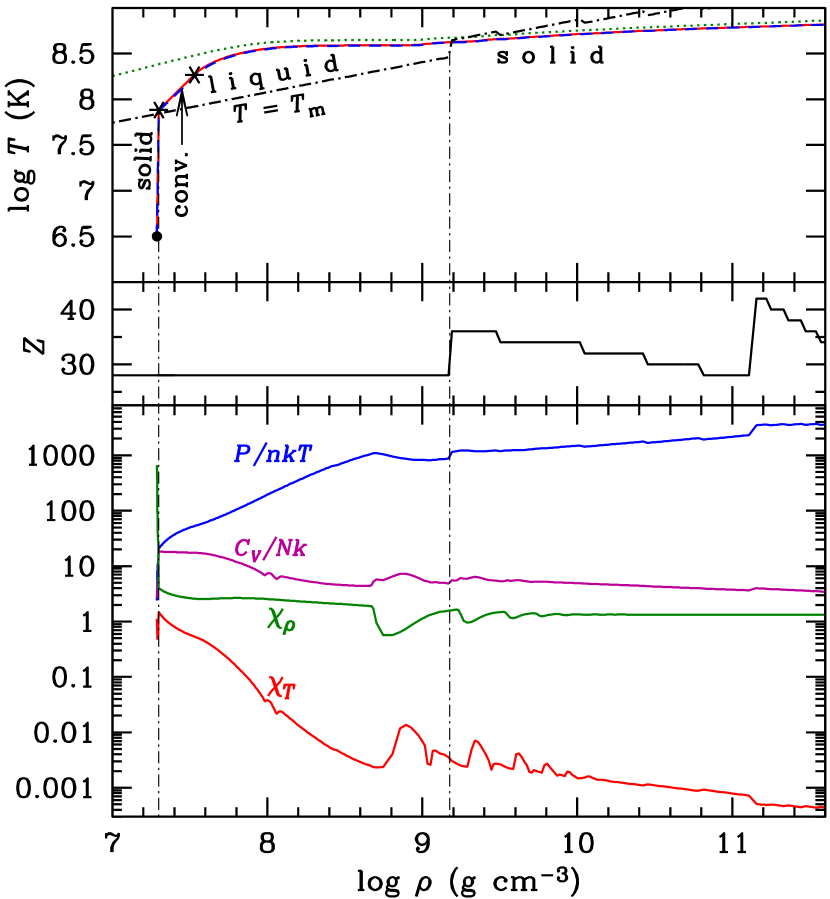
Figure 8: Structure of a magnetar envelope having the ground-state nuclear composition, the effective temperature $10^{6.5}$ K, and magnetic field $B=10^{15}$ G, inclined at $45^{\circ}$ to the surface. Top panel: thermal profiles calculated using the present EOS (solid red line) and the EOSs where the Coulomb nonideality is either neglected (dotted green line) or treated without account of magnetic quantization (dashed blue line, which is superposed on the solid red line). The melting temperature is drawn by the oblique dot-dashed line. Thin vertical dot-dashed lines mark the points of phase transitions from solid to liquid and back to solid state. Asterisks mark the ends of the convective segment, which is indicated by the arrow. Middle panel: ion charge (Rüster et al. 2006). Bottom panel: reduced pressure, heat capacity, and logarithmic derivatives of pressure.

The temperature quickly grows at the solid surface and reaches the melting point at the depth $z\approx 7$ cm. Thus, at the given conditions, the liquid ocean of a magnetar turns out to be covered by a thin layer of “ice” (solid substance). We treat the solid crust as immobile, but the liquid layer below the “ice” is convective up to the depth $z\sim 1$ m. We treat the convective heat transport through this layer in the adiabatic approximation (Schwarzschild 1958). The change of the heat-transport mechanism from conduction to convection causes the break of the temperature profile at the melting point. We underline that this treatment is only an approximation. In reality, the superadiabatic growth of temperature can lead to a hydrostatic instability of the shell of “ice” and eventually to its cracking and fragmentation into turning-up “ice floes”. This can result in transient enhancements of the thermal luminosity of magnetars.

The temperature profile flattens with density increase, and the Coulomb plasma freezes again at the interface between the layers of ⁶⁶Ni and ⁸⁶Kr at $\rho=1.5\times 10^{9}$ g cm^-3 ($z=73.8$ m). These phase transitions do not cause any substantial breaks in $\chi_{\rho}$, $\chi_{T}$, or $C_{V}/N_{\mathrm{i}}k_{\mathrm{B}}$, because the Coulomb plasmas have similar structure factors in the liquid and crystalline phases in the melting region (cf. Baiko et al. 1998).

At the boundaries between layers composed of different chemical elements, the reduced thermodynamic functions do not exhibit substantial discontinuities, except for the abrupt increases in $P/n_{\mathrm{i}}k_{\mathrm{B}}T$ at the interfaces ⁶⁶Ni/⁸⁶Kr ($\rho=1.5\times 10^{9}$ g cm^-3) and ⁷⁸Ni/¹²⁴Mo ($\rho=1.32\times 10^{11}$ g cm^-3), which are caused by the decreases in $n_{\mathrm{i}}$ with the large jumps in $A$ (of course, the non-normalized pressure $P$ is continuous). The specific heat per ion $C_{V}/N_{\mathrm{i}}k_{\mathrm{B}}$ is almost continuous at these interfaces, which means that heat capacity of unit volume abruptly decreases. The drop in $\chi_{T}$ at the ⁷⁸Ni/¹²⁸Mo interface is due to the same decrease in $n_{\mathrm{i}}$, which leads to the decrease in the ionic contribution that mostly determines $\partial P/\partial T$ at the strong degeneracy.

The oscillations of the reduced thermodynamic functions (most noticeable for $\chi_{\rho}$ and $\chi_{T}$) correspond to consecutive population of excited Landau levels by degenerate electrons with density increase, analogous to the oscillations in Fig. 6.

The magnetic effects on the nonideal part of the plasma thermodynamic functions have almost no influence on the temperature profile in the magnetar envelope, as illustrated in the upper panel of Fig. 8 where the corresponding solid and dashed lines virtually coincide. For comparison, the dotted line in the upper panel shows the result of a calculation totally neglecting the Coulomb nonideality. In this case, the profile is quite different at low densities, where there is no longer a solid surface. However, even in this case the thermal profile is almost the same at large $\rho$. This means that the Coulomb nonideality has a minor impact on the relation between the internal and effective temperatures and therefore on the cooling curves (Yakovlev & Pethick 2004), but it can be important for the shape of the thermal spectrum (cf., e.g., Potekhin et al. 2012).

8 Conclusions

We have systematically reviewed analytical approximations for the EOS of fully-ionized electron-ion plasmas in magnetic fields and described several improvements to the previously published approximations, taking nonideality attributable to ion-ion, electron-electron, and electron-ion interactions into account. The presented formulae are applicable in a wide range of plasma parameters, including the domains of nondegenerate and degenerate, nonrelativistic and relativistic electrons, weakly and strongly coupled Coulomb liquids, classical and quantum Coulomb crystals. As an application, we have calculated and discussed the behavior of thermodynamic functions, melting, and latent heat at crystallization of strongly coupled Coulomb plasmas with the parameters appropriate for cooling white dwarfs and envelopes of nonmagnetized and strongly magnetized neutron stars. We have also shown that a typical outer envelope of a magnetar can have a liquid layer beneath the solid surface.

The Fortran code that realizes the analytical approximations described in this paper is available at http://www.ioffe.ru/astro/EIP/ and at the CDS via anonymous ftp to cdsarc.u-strasbg.fr (130.79.128.5) or via http://cdsweb.u-strasbg.fr/cgi-bin/qcat?J/A+A/.

Appendix A Nonideal part of the free energy of electrons

Tanaka et al. (1985) calculated the interaction energy of the electron fluid at finite $T$ and presented a fitting formula that reproduced their numerical results as well as the results of other authors in various limits. Subsequently the behavior of the fit at $T\ll T_{\mathrm{F}}$ was improved by Ichimaru et al. (1987). The result reads

$$\frac{F_{ee}}{k_{\mathrm{B}}TN_{\mathrm{e}}}=-g\Gamma_{\mathrm{e}}-\frac{2A}{f}\,\sqrt{\Gamma}_{\mathrm{e}}$$

$$+\frac{2(dB+CA)}{fD}\left[\arctan\!\left(\!\frac{2f\,\sqrt{\Gamma}_{\mathrm{e}}+d}{D}\!\right)\!-\arctan\!\left(\frac{d}{D}\!\right)\right]$$

$$-\left(\frac{B}{f}-\frac{dA}{f^{2}}\right)\ln(f\Gamma_{\mathrm{e}}+d\sqrt{\Gamma}_{\mathrm{e}}+1),$$ (87)

where $A=b-gd$, $B=a-g$, $C=2-d^{2}/f$, $D=\sqrt{4f-d^{2}}$, and $a$, $b$, $d$, $f$, and $g$ are the following functions of $\theta=T/T_{\mathrm{F}}$ (at $B=0$):

$$a = \left(\frac{9}{4\pi^{2}}\right)^{1/3}\tanh\frac{1}{\theta}$$

$$\times\frac{0.75+3.04363\theta^{2}-0.09227\theta^{3}+1.7035\theta^{4}}{1+8.31051\theta^{2}+5.1105\theta^{4}}\,,$$

$$b = \frac{0.341308+12.0708\,\theta^{2}+1.148889\,\theta^{4}}{1+10.495346\,\theta^{2}+1.326623\,\theta^{4}}\sqrt{\theta}\,\tanh\frac{1}{\sqrt{\theta}}\,,$$

$$d = \!\!\frac{0.614925+16.996055\theta^{2}+1.489056\theta^{4}}{1+10.10935\,\theta^{2}+1.22184\,\theta^{4}}\sqrt{\theta}\,\tanh\frac{1}{\sqrt{\theta}}\,,$$

$$f = \frac{0.539409+2.522206\,\theta^{2}+0.178484\,\theta^{4}}{1+2.555501\,\theta^{2}+0.146319\,\theta^{4}}\,\theta\,\tanh\frac{1}{\,\theta}\,,$$

$$g = 0.872496+0.025248\,\exp(-1/\theta).$$

The accuracy of Eq. 87 is 1%.

In a quantizing magnetic field, we replace the argument $\theta$ in these expressions by the quantity $\theta^{\ast}$ defined by Eq. 74, as explained in Sect. 5.1.

Appendix B Nonideal part of the free energy of ions in the rigid background

B.1 Coulomb liquid

For the reduced free energy $f_{\mathrm{ii}}\equiv{F_{\mathrm{ii}}}/{N_{\mathrm{i}}k_{\mathrm{B}}T}$ of the classic OCP, we have the following analytical formula (Paper I):

$$f_{\mathrm{ii}}^{(0)} = A_{1}\Big{[}\sqrt{\Gamma(A_{2}+\Gamma)}-A_{2}\ln\!\left(\sqrt{\Gamma/A_{2}}+\sqrt{1+\Gamma/A_{2}}\right)\Big{]}$$ (88)

$$+2A_{3}\left[\sqrt{\Gamma}-\arctan\sqrt{\Gamma}\right]$$

$$+ \!\!\!B_{1}\left[\Gamma-B_{2}\ln\left(1+\frac{\Gamma}{B_{2}}\right)\right]+\frac{B_{3}}{2}\,\ln\left(1+\frac{\Gamma^{2}}{B_{4}}\right),$$

where $A_{1}=-0.907347$, $A_{2}=0.62849$, $B_{1}=0.0045$, $B_{2}=170$, $B_{3}=-8.4\times 10^{-5}$, $B_{4}=0.0037$, and $A_{3}=-\sqrt{3}/2-A_{1}/\sqrt{A_{2}}$. The derivative

$$\frac{\partial f_{\mathrm{ii}}^{(0)}}{\partial\ln\Gamma}=\Gamma^{3/2}\left[\frac{A_{1}}{\sqrt{\Gamma+A_{2}}}+\frac{A_{3}}{\Gamma+1}\right]+\frac{B_{1}\,\Gamma^{2}}{\Gamma+B_{2}}+\frac{B_{3}\,\Gamma^{2}}{\Gamma^{2}+B_{4}},$$ (89)

reproduces Monte Carlo calculations of the reduced internal energy ${U_{\mathrm{ii}}}/{N_{\mathrm{i}}k_{\mathrm{B}}T}$ at $1\leq\Gamma\leq 190$ (Caillol 1999) within the accuracy of these calculations, $\lesssim 10^{-3}$. For any values of the coupling parameter in a liquid OCP, $0\leqslant\Gamma\lesssim 200$, the fractional error of the approximation (88) does not exceed $2\times 10^{-4}$.

The classical treatment of ion motion is justified at $T\gg T_{\mathrm{p}}$. One can extend the applicability range of the analytical EOS to $T\sim T_{\mathrm{p}}$ by the Wigner-Kirkwood quantum corrections (Wigner 1932; Landau & Lifshitz 1980). The lowest-order correction to the reduced free energy is

$$f_{\mathrm{ii}}^{(2)}=\eta^{2}/24.$$ (90)

The next-order correction $\propto\hbar^{4}$ was obtained by Hansen & Vieillefosse (1975). It can be written as

$$f_{\mathrm{ii}}^{(4)} \approx \bigg{(}\!-2.085\times 10^{-4}-\frac{2.411\times 10^{-4}}{\Gamma^{1/2}}-\frac{0.001288}{\Gamma}$$ (91)

$$+\frac{1.353\times 10^{-4}}{\Gamma^{3/2}}-\frac{0.002476}{\Gamma^{2}}-\frac{0.00276}{\Gamma^{5/2}}\bigg{)}\,\eta^{4}.$$

This expression, unlike Eq. 90, is not exact. Both corrections have limited applicability, because as soon as $\eta$ becomes large, the Wigner expansion diverges and the plasma forms a quantum liquid, whose free energy is not known in an analytical form. Therefore we use only the lowest-order correction (90), i.e., $f_{\mathrm{ii}}\approx f_{\mathrm{ii}}^{(0)}+f_{\mathrm{ii}}^{(2)}$. In a magnetic field, Eq. 90 is replaced by Eq. 75 (Sect. 5.2).

B.2 Coulomb crystal

The reduced free energy of an OCP in the crystalline phase is given by Eq. 32, where the first three terms describe the harmonic lattice model (Baiko et al. 2001). For the bcc crystal, we have $C_{0}=-0.895\,929\,255\,68$ and $u_{1}=0.511\,3875$, and for $f_{\mathrm{th}}$ the following fitting formula can be used:

$$f_{\mathrm{th}}=\sum_{k=1}^{3}\ln\left(1-e^{-\alpha_{k}\eta}\right)-\frac{A(\eta)}{B(\eta)},$$ (92)

where $\alpha_{1}=0.932446$, $\alpha_{2}=0.334547$, $\alpha_{3}=0.265764$,

$$A(\eta) = 1+0.1839\,\eta+0.593\,586\,\eta^{2}+0.005\,4814\,\eta^{3}$$

$$+5.018\,13\times 10^{-4}\,\eta^{4}+3.9247\times 10^{-7}\,\eta^{6}$$

$$+5.8356\times 10^{-11}\,\eta^{8},$$

$$B(\eta) = 261.66+7.079\,97\,\eta^{2}+0.0409\,484\,\eta^{4}$$

$$+3.973\,55\times 10^{-4}\,\eta^{5}+5.111\,48\times 10^{-5}\,\eta^{6}$$

$$+2.197\,49\times 10^{-6}\,\eta^{7}+1.866\,985\times 10^{-9}\,\eta^{9}$$

$$+2.787\,72\times 10^{-13}\,\eta^{11}.$$

The Taylor expansion of Eq. 92 at small $\eta$ is consistent with the Wigner correction 90. However, the next Taylor term $\sim\eta^{3}$ is absent in the Wigner expansion, and therefore Eq. 92 does not reproduce higher-order Wigner corrections. Nevertheless, approximation 92 is very accurate: it reproduces the numerical results in Baiko et al. (2001) with fractional deviations within $5\times 10^{-6}$, and its first and second derivatives reproduce the calculated contributions to the internal energy and heat capacity with deviations up to several parts in $10^{5}$. Other types of simple lattices are described by the same expressions with slightly different parameters (see Baiko et al. 2001).

Anharmonic corrections for Coulomb lattices were studied in a number of works (see Papers I and II for references). In the classical regime $\eta\to 0$, we have chosen one of the 11 parametrizations proposed by Farouki & Hamaguchi (1993):

$$f_{\mathrm{ah}}^{(0)}(\Gamma)=-\sum_{k=1}^{3}\frac{a_{k}}{k\Gamma^{k}},$$ (93)

where $a_{1}=10.9$, $a_{2}=247$, and $a_{3}=1.765\times 10^{5}$. A continuation to arbitrary $\eta$, which is consistent with available analytical and numerical results for quantum crystals, reads (Paper II)

$$f_{\mathrm{ah}}=f_{\mathrm{ah}}^{(0)}(\Gamma)\,e^{-0.0112\eta^{2}}-0.12\,\eta^{2}/\Gamma\,.$$ (94)

Superstrong magnetic fields can significantly change these expressions under the conditions $\zeta_{\mathrm{i}}\gtrsim 1$ and $\eta\gtrsim 1$. Analytical approximations for the free energy of a harmonic Coulomb crystal in quantizing magnetic fields are derived in Sect. 6. Analogous results for the anharmonic corrections are currently unavailable.

Appendix C Electron polarization corrections

C.1 Coulomb liquid

The screening contribution to the reduced free energy of the Coulomb liquid at $0<\Gamma\lesssim 300$ has been calculated by the HNC technique and fitted by the expression (Paper I)

$$f_{\mathrm{ie}}\equiv\frac{F_{\mathrm{ie}}}{N_{\mathrm{i}}k_{\mathrm{B}}T}=-\Gamma_{\mathrm{e}}\,\frac{c_{\mathrm{DH}}\sqrt{\Gamma_{\mathrm{e}}}+c_{\mathrm{TF}}a\Gamma_{\mathrm{e}}^{\nu}g_{1}h_{1}}{1+\left[b\,\sqrt{\Gamma_{\mathrm{e}}}+ag_{2}\Gamma_{\mathrm{e}}^{\nu}/r_{\mathrm{s}}\right]\gamma_{\mathrm{r}}^{-1}},$$ (95)

where $c_{\mathrm{DH}}=(Z/\sqrt{3})\left[(1+Z)^{3/2}-1-Z^{3/2}\right]$ ensures exact transition to the Debye-Hückel limit at $\Gamma\to 0$, $c_{\mathrm{TF}}=(18/175)\,(12/\pi)^{2/3}Z^{7/3}\left(1-Z^{-1/3}+0.2\,Z^{-1/2}\right)$ fits the numerical data at large $\Gamma$ and reproduces the Thomas-Fermi limit (Salpeter 1961) at $Z\to\infty$, the parameters $a=1.11\,Z^{0.475}$, $b=0.2+0.078\,(\ln Z)^{2},$ and $\nu=1.16+0.08\ln Z$ provide a low-order approximation to $F_{ie}$ for intermediate $r_{\mathrm{s}}$ and $\Gamma$. The functions

$$g_{1} = 1+0.78\left[21+\Gamma_{\mathrm{e}}(Z/r_{\mathrm{s}})^{3}\right]^{-1}(\Gamma_{\mathrm{e}}/Z)^{1/2},$$

$$g_{2} = 1+\frac{Z-1}{9}\left(1+\frac{1}{0.001\,Z^{2}+2\Gamma_{\mathrm{e}}}\right)\frac{r_{\mathrm{s}}^{3}}{1+6\,r_{\mathrm{s}}^{2}}\,,$$

improve the fit at relatively large $r_{\mathrm{s}}$. Finally, the function

$$h_{1}=\frac{1+x_{\mathrm{r}}^{2}/5}{1+0.18\,Z^{-1/4}x_{\mathrm{r}}+0.37\,Z^{-1/2}x_{\mathrm{r}}^{2}+x_{\mathrm{r}}^{2}/5}$$

is the relativistic correction, as is $\gamma_{\mathrm{r}}^{-1}$ in the denominator.

C.2 Coulomb crystal

The screening contribution to the reduced free energy of the Coulomb crystals was evaluated using the semiclassical perturbation approach with an effective structure factor (Paper I) and fitted by the expression (Paper II)

$$f_{\mathrm{ie}}=-f_{\infty}(x_{\mathrm{r}})\,\Gamma\left\{1+A(x_{\mathrm{r}})\,\big{[}Q(\eta)/\Gamma\big{]}^{s}\right\},$$ (96)

where

$$f_{\infty}(x) = a_{\mathrm{TF}}Z^{2/3}b_{1}\,\sqrt{1+b_{2}/x^{2}},$$

$$A(x) = \frac{b_{3}+17.9x^{2}}{1+b_{4}x^{2}},$$

$$Q(\eta) = \left[{\ln\left(1+e^{(0.205\eta)^{2}}\right)}\right]^{1/2}\,\left[{\ln\left(e-(e-2)e^{-(0.205\eta)^{2}}\right)}\right]^{-1/2},$$

the parameter $a_{\mathrm{TF}}=0.00352$ is related to $c_{\mathrm{TF}}$ in Eq. 95, and parameters $s$ and $b_{1}$ – $b_{4}$ depend on $Z$:

$$s = \left[1+0.01\,(\ln Z)^{3/2}+0.097\,Z^{-2}\right]^{-1},$$

$$b_{1} = 1-1.1866\,Z^{-0.267}+0.27\,Z^{-1},$$

$$b_{2} = 1+\frac{2.25}{Z^{1/3}}\,\frac{1+0.684\,Z^{5}+0.222\,Z^{6}}{1+0.222\,Z^{6}},$$

$$b_{3} = 41.5/(1+\ln Z),$$

$$b_{4} = 0.395\ln Z+0.347\,Z^{-3/2}.$$

Here, the numerical parameters are given for the bcc crystal; their values for the fcc lattice are slightly different (Paper I).

References

- Alastuey & Jancovici (1980) Alastuey, A., & Jancovici, B. 1980, Physica A, 102, 327
- Baiko (2000) Baiko, D. A. 2000, PhD thesis (St. Petersburg: Ioffe Phys.-Tech. Inst.) [in Russian]
- Baiko (2002) Baiko, D. A. 2002, Phys. Rev. E, 66, 056405
- Baiko (2009) Baiko, D. A. 2009, Phys. Rev. E, 80, 046405
- Baiko & Yakovlev (2012) Baiko, D. A., & Yakovlev, D. G. 2012, private communication
- Baiko et al. (1998) Baiko, D. A., Kaminker, A. D., Potekhin, A. Y., & Yakovlev, D. G. 1998, Phys. Rev. Lett., 81, 5556
- Baiko et al. (2001) Baiko, D. A., Potekhin, A. Y., & Yakovlev, D. G. 2001, Phys. Rev. E, 64, 057402
- Banerjee et al. (1974) Banerjee, B., Constantinescu, D. H., & Rehak, P. 1974, Phys. Rev. D, 10, 2384
- Berestetskiĭ et al. (1982) Berestetskiĭ, V. B., Lifshitz, E. M., & Pitaevskiĭ, L. P., 1982, Quantum Electrodynamics (Oxford: Butterworth-Heinemann)
- Blandford & Hernquist (1982) Blandford, R. D., & Hernquist, L. 1982, J. Phys. C: Solid State Phys., 15, 6233
- Blinnikov et al. (1996) Blinnikov, S. I., Dunina-Barkovskaya, N. V. Nadyozhin, D. K. 1996, ApJS, 106 171; erratum: 1998, ApJS, 118, 603
- Brami et al. (1979) Brami, B., Hansen, J. P., & Joly, F. 1979, Physica, 95A, 505
- Broderick et al. (2000) Broderick, A., Prakash, M. & Lattimer, J. M. 2000, ApJ, 537, 351
- Caillol (1999) Caillol, J. M. 1999, J. Chem. Phys., 111, 6538
- Canuto & Chiu (1968) Canuto, V., & Chiu, H.-Y. 1968, Phys. Rev., 173, 1220
- Chabrier & Ashcroft (1990) Chabrier G., & Ashcroft, N. W. 1990, Phys. Rev. A, 42, 2284
- Chabrier & Baraffe (2000) Chabrier G., & Baraffe, I. 2000, ARA&A, 38, 337
- Chabrier & Potekhin (1998) Chabrier, G., & Potekhin, A. Y. 1998, Phys. Rev. E, 58, 4941
- Chabrier et al. (2002) Chabrier, G., Douchin, F., & Potekhin, A. Y. 2002, J. Phys.: Condensed Matter, 14, 9133
- Chandrasekhar (1957) Chandrasekhar, S. 1957, An Introduction to the Study of Stellar Structure (New York: Dover, 1957), Chap. X.
- Cornu (1998) Cornu, F. 1998, Phys. Rev. E, 58, 5293
- Danz & Glasser (1971) Danz, R. W., & Glasser, M. L. 1971, Phys. Rev. B, 4, 94
- DeWitt et al. (1996) DeWitt, H. E., Slattery, W., & Chabrier, G. 1996, Physica A, 228, 21
- DeWitt & Slattery (2003) DeWitt, H. E., & Slattery, W. 2003, Contrib. Plasma Phys., 43, 279
- Farouki & Hamaguchi (1993) Farouki, R. T., & Hamaguchi, S. 1993, Phys. Rev. E, 47, 4330
- Fortov (2009) Fortov, V. E. 2009, Phys. Usp., 52, 615
- Fushiki et al. (1989) Fushiki, I., Gudmundsson, E. H., & Pethick, C. J. 1989, ApJ, 342, 958
- Galam & Hansen (1976) Galam S., & Hansen, J. P. 1976, Phys. Rev. A, 14, 816
- Girifalco (1973) Girifalco, L. A. 1973, Statistical Physics of Materials (New York: Wiley-Interscience, 1973), App. V.
- Griffith (1999) Griffith, D. J. 1999, Introduction to Electrodynamics, 3rd ed. (London: Prentice-Hall), Chap. 6.
- Haensel et al. (2007) Haensel, P., Potekhin, A. Y., & Yakovlev, D. G. 2007, Neutron Stars 1: Equation of State and Structure (New York: Springer)
- Hamaguchi et al. (1997) Hamaguchi, S., Farouki, R. T., & Dubin, D. H. E. 1997, Phys. Rev. E, 56, 4671
- Hansen (2004) Hansen, B. M. S. 2004, Phys. Rep., 399, 1
- Hansen et al. (1977) Hansen, J. P., Torrie, G. M., & Vieillefosse, P. 1977, Phys. Rev. A, 16, 2153
- Hansen & Vieillefosse (1975) Hansen, J. P., & Vieillefosse, P. 1975, Phys. Lett. A, 53, 187
- Hughto et al. (2012) Hughto, J., Horowitz, C. J., Schneider, A. S., et al. 2012, Phys. Rev. E, accepted (arXiv:1211.0891)
- Ichimaru et al. (1987) Ichimaru, S., Iyetomi, H., & Tanaka, S. 1987, Phys. Rep., 149, 91
- Jancovici (1962) Jancovici, B. 1962, Nuovo Cimento, 25, 428
- Johnson & Lippmann (1949) Johnson, M. H., & Lippmann, B. A. 1949, Phys. Rev., 76, 828
- Kaplan & Glasser (1972) Kaplan, J. L., & Glasser, M. L. 1972, Phys. Rev. Lett., 28, 1077
- Kittel (1963) Kittel, C., 1963, Quantum Theory of Solids (New York: Wiley).
- Lai (2001) Lai, D. 2001, Rev. Mod. Phys., 73, 629
- Lai & Salpeter (1997) Lai, D., & Salpeter, E. E. 1997, ApJ, 491, 270
- Landau (1930) Landau, L. D. 1930, Z. f. Physik, 64, 629
- Landau & Lifshitz (1977) Landau, L. D., & Lifshitz, E. M. 1977, Quantum Mechanics. Non-Relativistic Theory, 3rd ed. (Oxford: Pergamon)
- Landau & Lifshitz (1980) Landau, L. D., & Lifshitz, E. M. 1980, Statistical Physics, Part 1, 3rd ed. (Oxford: Butterworth-Heinemann)
- Medin (2012) Medin, Z. 2012, private communication
- Medin & Cumming (2010) Medin, Z., & Cumming, A. 2010, Phys. Rev. E, 81, 036107
- Medin & Lai (2006) Medin, Z., & Lai, D. 2006, Phys. Rev. A, 74, 062508
- Medin & Lai (2007) Medin, Z., & Lai, D. 2007, MNRAS, 382, 1833
- Militzer & Graham (2006) Militzer, B., & Graham, R. L. 2006, J. Phys. Chem. Sol. 67, 2136
- Morbec & Capelle (2008) Morbec, J. M., & Capelle, K. 2008, Phys. Rev. B, 78, 085107
- Nagai & Fukuyama (1982) Nagai, T., & Fukuyama, H. 1982, J. Phys. Soc. Japan, 51, 3431
- Nagai & Fukuyama (1983) Nagai, T., & Fukuyama, H. 1983, J. Phys. Soc. Japan, 52, 44
- Ogata et al. (1993) Ogata, S., Iyetomi, H., Ichimaru, S., & Van Horn, H. M. 1993, Phys. Rev. E, 48, 1344
- Paxton et al. (2011) Paxton, B., Bildsten, L., Dotter, A., et al. 2011, ApJS, 192, 3
- Pollock & Hansen (1973) Pollock, E. L., & Hansen, J. P. 1973, Phys. Rev. A, 8, 3110
- Potekhin & Chabrier (2000) Potekhin, A. Y., & Chabrier, G. 2000, Phys. Rev. E, 62, 8554 (Paper I)
- Potekhin & Chabrier (2004) Potekhin, A. Y., & Chabrier, G. 2004, ApJ, 600, 317
- Potekhin & Chabrier (2010) Potekhin, A. Y., & Chabrier, G. 2010, Contrib. Plasma Phys., 50, 82 (Paper II)
- Potekhin et al. (1999) Potekhin, A. Y., Chabrier, G., & Shibanov, Yu. A. 1999, Phys. Rev. E, 60, 2193
- Potekhin et al. (2007) Potekhin, A. Y., Chabrier, G., & Yakovlev, D. G. 2007, Ap&SS, 308, 353 (electronic version with corrected misprints: arXiv:astro-ph/0611014v3)
- Potekhin et al. (2009a) Potekhin, A. Y., Chabrier, G., & Rogers, F. J. 2009a, Phys. Rev. E, 79, 016411
- Potekhin et al. (2009b) Potekhin, A. Y., Chabrier, G., Chugunov, A. I., DeWitt, H. E., & Rogers, F. J. 2009b, Phys. Rev. E, 80, 047401
- Potekhin et al. (2012) Potekhin, A. Y., Suleimanov, V. F., van Adelsberg, M., & Werner, K. 2012, A&A, 546, A121
- Rögnvaldsson et al. (1993) Rögnvaldsson, Ö. E., Fushiki, I., Gudmundsson, E. H., Pethick, C. J., & Yngvason, J. 1993, ApJ, 416, 276
- Rosenfeld (1996) Rosenfeld, Y. 1996, Phys. Rev. E, 54, 2827
- Ruderman (1971) Ruderman, M. A. 1971, Phys. Rev. Lett., 27, 1306
- Rüster et al. (2006) Rüster, S. B., Hempel, M., & Schaffner-Bielich, J. 2006, Phys. Rev. C, 73, 035804
- Salpeter (1961) Salpeter, E. E. 1961 ApJ, 134, 669
- Schwarzschild (1958) Schwarzschild, M. 1958, Structure and Evolution of the Stars (Princeton: Princeton Univ. Press)
- Schwinger (1988) Schwinger, J. 1988, Particles, Sources, and Fields (Redwood: Addison-Wesley)
- Sharma & Reddy (2011) Sharma, R., & Reddy, S. 2011, Phys. Rev. C, 83, 025803
- Steinberg et al. (1998) Steinberg, M., Ortner, J., & Ebeling, W. 1998, Phys. Rev. E, 58, 3806
- Steinberg et al. (2000) Steinberg, M., Ebeling, W., & Ortner, J. 2000, Phys. Rev. E, 61, 2290
- Suh & Mathews (2001) Suh, I.-S., & Mathews, G. J. 2001, ApJ, 546, 1126
- Tanaka et al. (1985) Tanaka, S., Mitake, S., & Ichimaru, S. Phys. Rev. A, 32, 1896
- Thorolfsson et al. (1998) Thorolfsson, A., Rögnvaldsson, Ö. E., Yngvason, J., & Gudmundsson, E. H. 1998, ApJ, 502, 847
- Timmes & Arnett (1999) Timmes, F. X., & Arnett, D. 1999, ApJS, 125, 277
- Timmes & Swesty (2000) Timmes, F. X., & Swesty, F. D. 2000, ApJS, 126, 501
- Usov et al. (1980) Usov, N. A., Grebenshchikov, Yu. B., & Ulinich, F. R. 1980, Sov. Phys.–JETP, 51, 148
- van Leeuwen (1921) van Leeuwen, J. H. 1921, J. de Physique et le Radium, Ser. VI, 2, 361
- Wickramasinghe & Ferrario (2000) Wickramasinghe, D. T., & Ferrario, L. 2000, PASP, 112, 873
- Wigner (1932) Wigner, E. P. 1932, Phys. Rev. 40, 749
- Yakovlev & Kaminker (1994) Yakovlev, D. G., & Kaminker, A. D. 1994, in The Equation of State in Astrophysics, Proceedings of IAU Colloquium No. 147, ed. G. Chabrier & E. Schatzman (Cambridge: Cambridge University Press), 214
- Yakovlev & Pethick (2004) Yakovlev, D. G., & Pethick, C. J. 2004, ARA&A, 42, 169
- Yakovlev & Shalybkov (1989) Yakovlev, D. G. & Shalybkov, D. A. 1989, Astrophys. Space Phys. Rev. 7, 311