A Parameterized Approximation Algorithm for The Shallow-Light Steiner Tree Problem

Abstract

For a given graph $G=(V,\,E)$ with a terminal set $S$ and a selected root $r\in S$, a positive integer cost and a delay on every edge and a delay constraint $D\in Z^{+}$, the shallow-light Steiner tree (SLST) problem is to compute a minimum cost tree spanning the terminals of $S$, in which the delay between root and every vertex is restrained by $D$. This problem is NP-hard and very hard to approximate. According to known inapproximability results, this problem admits no approximation with ratio better than factor $(1,\,O(\log^{2}n))$ unless $NP\subseteq DTIME(n^{\log\log n})$ [10], while it admits no approximation ratio better than $(1,\,O(\log|V|))$ for $D=4$ unless $NP\subseteq DTIME(n^{\log\log n})$ [2]. Hence, the paper focus on parameterized algorithm for SLST. We firstly present an exact algorithm for SLST with time complexity $O(3^{|S|}|V|D+2^{|S|}|V|^{2}D^{2}+|V|^{3}D^{3})$, where $|S|$ and $|V|$ are the number of terminals and vertices respectively. This is a pseudo polynomial time parameterized algorithm with respect to the parameterization: “number of terminals”. Later, we improve this algorithm such that it runs in polynomial time $O(\frac{|V|^{2}}{\epsilon}3^{|S|}+\frac{|V|^{4}}{\epsilon}2^{|S|}+\frac{|V|^{6}}{\epsilon})$ , and computes a Steiner tree with delay bounded by $(1+\epsilon)D$ and cost bounded by the cost of an optimum solution, where $\epsilon>0$ is any small real number. To the best of our knowledge, this is the first parameterized approximation algorithm for the SLST problem.

hallow light Steiner tree, parameterized approximation algorithm, directed Steiner tree, exact algorithm, auxiliary graph, pseudo-polynomial time complexity.

1 Introduction

The well-known shallow-light Steiner tree problem (or namely the delay restrained minimum Steiner tree problem) is defined as below:

Definition 1

For a graph $G=(V,\,E)$ with a terminal set $S$, a root vertex $r\in S$, a cost function $c:\,E\rightarrow Z^{+}$, a delay function $d:\,E\rightarrow Z^{+}$, and a delay bound $D\in Z^{+}$, the shallow-light Steiner tree (SLST) problem is to compute a minimum cost Steiner tree $slst$ spanning all terminals of $S$, such that the delay from $r$ to every terminal in $slst$ is not larger than $D$.

For notation briefness, we assume $|V|=n,\,|E|=m,\,|S|=t$ in graph $G$, and use SLST and $slst$ to denote the shallow-light Steiner tree problem and an optimal shallow-light Steiner tree respectively. For the SLST problem, bifactor approximation algorithms have been developed.

Definition 2

An algorithm $A$ is a bifactor $\left(\alpha,\,\beta\right)$-approximation for the SLST problem, if and only if for every instance of SLST, $A$ computes a Steiner tree $slst$ in polynomial time, such that the delay from $r$ to every terminal in $slst$ is bounded by $\alpha*D$ and the cost of $Slst$ is bounded by $\beta$ times of the cost of the optimal solution.

Noting that single factor $\beta$-approximation is identical to bifactor $\left(1,\,\beta\right)$-approximation for SLST, we use them interchangeably in the text.

Related Work. It is known that the SLST problem is NP-hard, and can not be approximated better than factor $(1,\,O(\log^{2}n))$ unless $NP\subseteq DTIME(n^{\log\log n})$ [10]. This is because the group Steiner tree problem can be embedded into this problem. Furthermore, no polylogarithmic approximation within polynomial time complexity has been developed. The best work is a long standing result due to Charikar et al, which is a polylogarithmic approximation in quasi-polynomial time, i.e. factor-$O(\log^{2}t)$ approximation within time complexity $n^{O(\log t)}$[3]. Due to the difficulty in single factor approximation algorithm design, bifactor approximation has been investigated. Hajiaghayi et al presented an $(O(\log^{2}t),\,O(\log^{4}t))$-approximation algorithm that runs in polynomial time [8]. Besides, Kapoor and Sarwat gave an approximation with bifactor $(O(\frac{p\log t}{\log p}),O(\frac{\log t}{\log p}))$, where $p$ is an input parameter [9]. The last algorithm is an approximation that improves the cost of the tree, and is with bifactor $(O(t),\,O(1))$ when $p=t$ [9].

The SLST problem remains hard to approximate even when $S=V$. In that case, this problem becomes the shallow light spanning tree (SLT) problem, which has broad applications in network design, VLSI and etc. For computational complexity, the SLT problem is claimed to be with inapproximability hardness of $(1,\,\Omega(\log n))$ [12]. For approximation, Charikar et al’s $O(\log^{2}n)$ ratio with time complexity $n^{O(\log n)}$[3] is still the best single factor result. Naor and Schieber gave an approximation bifactor of $(2,\,O(\log n))$, i.e. with delay and cost bounded by 2 times and $O(\log n)$ times of that of the optimal solution respectively [12]. To the best of our knowledge, these are the best long standing approximation ratios. Some special cases of the SLT problem are also interesting. If edge cost is equal to the delay for each edge, the SLT problem remains NP-hard and admit no approximation algorithms with bifactor $(\alpha,\,\beta)$ for any $\alpha>1$ and $1\leq\beta<1+\frac{2}{\alpha-1}$ [11], while the best possible result for SLST is a $(1+\epsilon,\,O(\log(\frac{1}{\epsilon})))$-approximation [5]. Moreover, the SLT problem remains NP-hard when all edge delays are equal, but polynomially solvable when all edge costs are equal [13]. For the equal-delay case, namely the hop constrained minimum spanning tree problem, Althaus et al have presented an approximation with a ratio of $(1,\,O(\log n))$ in [1].

Another two important special cases of the SLST problem is when $D$ is constant or when all edge delays are equal. Unfortunately, for the former case, SLST can not be approximated better than a factor of $(1,\,O(\log n))$ for even $D=4$ unless $NP\subseteq DTIME(n^{\log\log n})$ [2], since the Set Cover problem can be embedded into this case. Bar-Ila et al also developed a factor-$(1,\,O(\log n))$ approximation for the cases of $D=4,\,5$ in the same paper, achieving the best possible ratio. When all edge delays are equal, namely the hop constrained minimum Steiner tree problem, it is open that if there exists factor-$(1,\,O(\log n))$ approximation for this problem, as the spanning case.

Our Contribution. The first result of this paper is an exact algorithm, with time complexity $O(3^{|S|}|V|D+2^{|S|}|V|^{2}D^{2}+|V|^{3}D^{3})$, for the SLST problem. This result indicates that if the number of terminal and the delay constraint are bounded, the SLST problem is polynomial solvable. Our technique is mainly based on constructing an auxiliary graph, where every Steiner tree satisfies the delay constraint, i.e. in the auxiliary graph, we only need to compute Steiner tree without considering the delay constraint. Though its time complexity seems terrible, the exact algorithm is efficient for real-world applications for $|S|<80$, particularly when $D=o(n)$ or all edge delays are equal (the hop constrained minimum Steiner tree problem).

On the theoretical side, we note that this algorithm runs in pseudo polynomial time (for constant $|S|$), since $D$ appears in the formula of the time complexity. The second result is to improve this time complexity to polynomial time $O(\frac{|V|^{2}}{\epsilon}3^{|S|}+\frac{|V|^{4}}{\epsilon}2^{|S|}+\frac{|V|^{6}}{\epsilon})$ following a similar line of polynomial-time approximation scheme (PTAS) design, such that it computes a Steiner tree with delay bounded by $(1+\epsilon)D$ and cost bounded by the cost of an optimum solution.

2 A Parameterized Approximation Algorithm for the Shallow Light Steiner Problem

In this section we shall approximate the shallow-light Steiner tree (SLST) problem. Firstly and intuitively, our main observation is that the difficulty of computing a $slst$ comes from obeying the given delay constraint. Therefore, our key idea is to construct an auxiliary directed graph $H$ where there exists only cost (i.e. no delay) on edges, such that every Steiner tree (spanning the same terminal set) in $H$ corresponds to a Steiner tree that satisfies the given delay constraint $D$ in $G$. Secondly since the directed Steiner tree problem is known parameterized tractable with respect to the parameterization: “number of terminals”[6, 4], an exact algorithm is immediately obtained; then an approximation algorithm with ratio $(1+\epsilon,\,1)$ can be derived from the exact algorithm by a method of shrinking the value of $D$. The approximation algorithm computes a $slst$ with delay bounded by $D(1+\epsilon)$ and cost bounded by the cost of an optimum $slst$.

2.1 Construction of the Auxiliary Graph

Though different in technique details, the key idea to construct the auxiliary graph is similar to the auxiliary graph used to balance the cost and delay of $k$ disjoint shortest paths in [7]: using layer graphs. For a given graph $G=(V,E)$ with positive integer cost and delay on every edge, and a delay constraint $D$, the layer graph $H$, i.e. the auxiliary graph to be constructed, contains vertices, terminals and edges roughly as in the following:

1. $D$ vertices $v_{l}^{1},\dots,v_{l}^{D}$ corresponding to every vertex $v_{l}\in G$ ;

2. $D-d(e)$ edges $\left\langle v_{j}^{1},\,v_{l}^{d(e)+1}\right\rangle,\,\dots,\left\langle v_{j}^{D-d(e)},\,v_{l}^{D}\right\rangle$ corresponding to every edge $e=\left\langle v_{j},v_{l}\right\rangle\in E$ and with $c(\left\langle v_{j}^{i},\,v_{l}^{d(e)+i}\right\rangle)=c(e)$;

3. one terminal $v_{l}$, corresponding to every terminal $v_{l}\in S\subseteq G$, together with cost-0 edges $\{\left\langle v_{l}^{i},\,v_{l}\right\rangle|i=1,\dots,D\}$ that connect auxiliary vertices of $v_{l}$ to the auxiliary terminal;

Therefore, $H$ has $O(|V|*D)$ vertices, $O(|E|*D)$ edges, and $|S|$ terminals. The construction is formerly as in Algorithm 1 (An example of such construction is as depicted in Figure 1).

Input: Graph $G=(V,E)$, a set of terminals $S\subseteq V$, a root vertex $r\in S$, cost $c:\,e\rightarrow Z^{+}$and delay $d:\,e\rightarrow Z^{+}$ on every edge $e\in E$, and a delay constraint $D$;

Output: Auxiliary acyclic graph $H$ and the terminal set therein, $S_{H}$.

1. $H:=\{r\}$, $S_{H}:=\{r\}$;

2. For each $v_{l}\in V\setminus\{r\}$ do

   1. $H:=H\cup\{v_{l}^{1},\dots,v_{l}^{D}\}$;

   2. If $v_{l}\in S$ then

      1. $H:=H\cup\{v_{l}\}\cup\{\left\langle v_{l}^{i},\,v_{l}\right\rangle|i=1,\dots,D\}$, and set $c(\left\langle v_{l}^{i},\,v_{l}\right\rangle):=0$ for each $i$;

      2. $S_{H}:=S_{H}\cup\{v_{l}\}$;

3. For each $e=\left\langle v_{j},\,v_{l}\right\rangle\in E$ that $r\notin e$ do

   $H:=H\cup\{\left\langle v_{j}^{i},\,v_{l}^{d(e)+i}\right\rangle|i=1,\,\dots,\,D-d(e)\}$, and set $c(\left\langle v_{j}^{i},\,v_{l}^{d(e)+i}\right\rangle):=c(e)$ for each $i$;

4. For each $e=\left\langle r,v_{l}\right\rangle$ do

   $H:=H\cup\{\left\langle r,v_{l}^{d(e)}\right\rangle\}$, and set $c(\left\langle r,v_{l}^{d(e)}\right\rangle):=c(e)$ .

5. Return $H$ and $S_{H}$.

Algorithm 1 Construction of auxiliary graph $H$.

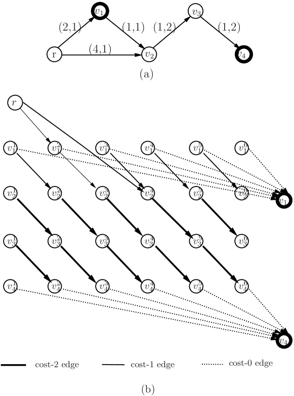
Figure 1: Construction of acyclic graphs: (a) is the original graph, in which $r,\,v_{1},\,v_{4}$ are terminals; (b) is the constructed auxiliary graph, in which $r,\,v_{1},\,v_{4}$ are terminals.

It remains to show that the $r$-rooted minimum cost directed Steiner tree in $H$ corresponds to a $r$-rooted minimum $slst$ in $G$.

Lemma 3

A minimum cost directed Steiner tree rooted at $r$ in $H$ contains at most one vertex of $\{v_{l}^{1},\dots,v_{l}^{D}\}$ for each $l$.

Proof

Let $R$ be a $r$-rooted minimum cost directed Steiner tree in $H$. Suppose $R$ contains $v_{l}^{j}$ and $v_{l}^{j+\Delta}$. Then we show that $R$ is not minimum and get a contradiction. Let $R^{\prime}$ be $R$ except removing the edge entering $v_{l}^{j+\Delta}$ and replacing every edge in the subtree of $R$ that roots at $v_{l}^{j+\Delta}$, say $\left\langle v_{h}^{i+\Delta},v_{h^{\prime}}^{i^{\prime}+\Delta}\right\rangle$ by edge $\left\langle v_{h}^{i},v_{h^{\prime}}^{i^{\prime}}\right\rangle$. Apparently, $R^{\prime}$ spanning the same terminal set as $R$. That is, there exists a directed Steiner tree $R^{\prime}$ with less cost than $R$ in $H$. This contradicts with the fact that $R$ is minimum.

Theorem 4

Let $S_{H}$ be the set of terminal vertices $\{v_{1},\dots,v_{t}\}$ in $H$. Then there exists a $r$-rooted directed Steiner tree spanning $S_{H}$ of minimum cost $C$ in $H$ iff there exists a Steiner tree spanning $S$ of minimum cost $C$ with delay between $r$ and every terminal restrained by $D$ in $G$.

Proof

Let $R$ be a minimum cost directed Steiner tree rooted at $r$ in $H$. Let $R^{\prime}$ be a subgraph of $G$, in which $e(v_{j},v_{l})\in R^{\prime}$ if and only if there exists $e(v_{j}^{i_{j}},v_{l}^{i_{l}})\in R$. Then because $c(v_{j},v_{l})=c(v_{j}^{i_{j}},v_{l}^{i_{l}})$, we have $c(R^{\prime})=c(R)$. It remains to show $R^{\prime}$ is a Steiner tree. From Lemma 3, $|\{v_{l}^{1},\dots,v_{l}^{D}\}\cap R|\leq 1$ holds for every $l$. So a path connecting $r$ to a terminal in $H$ corresponds to a path connecting $r$ to a terminal in $G$. Then since every terminal of $S_{H}$ is reachable from $r$ in $R$, all terminals of $S$ are connected to $r$ in $R^{\prime}$. Besides, because $R$ is a tree, $R^{\prime}$ contains no loops or parallel edges. Therefore, $R^{\prime}$ is a Steiner tree of $G$.

Let $R^{\prime}$ be a Steiner tree in $G$. Then there is a unique path from root $r$ to every other vertex of $R^{\prime}$. Hence, every vertex of $R^{\prime}$ has a unique delay from $r$. Let $R$ contains edge $(v_{j}^{d(v_{j})},v_{j})$ for every $v_{j}\in S_{H}$, and edge $(v_{j}^{d(v_{j})},v_{l}^{d(v_{j})+d(v_{j},v_{l})})$ if and only if $(v_{j},v_{l})\in R^{\prime}$, where $d(v_{j})$ is the delay from $r$ to $v_{j}$ in $R$ and $d(v_{j},v_{l})$ the delay from $v_{j}$ to $v_{l}$. Since the delay of from $r$ to every vertex in $R^{\prime}$ is not larger than $D$, edge $(v_{j}^{d(v_{j})},v_{l}^{d(v_{j})+d(v_{j},v_{l})})$ belongs to $H$, and hence $R\subseteq H$. Then because every $v_{j}\in R$ is reachable from $r$ and no loop or parallel edge exists following the construction of $R$, $R$ is a Steiner tree in $H$ with cost $c(R)\leq c(R^{\prime})$. This completes the proof.

2.2 A parameterized Approximation Algorithm for Shallow-Light Steiner Tree

This subsection shall give an exact algorithm and a parameterized approximation algorithm for the SLST problem. From Theorem 4, an algorithm for the SLST problem can be obtained by computing a minimum cost directed Steiner tree in $H$. Unfortunately, it is known that the (minimum) directed Steiner tree problem is NP-hard and maybe even more difficult to approximate than SLST, i.e. only a quasi-polynomial time algorithm with a polylogarithmic approximation factor has been developed[3]. However, when the number of the terminals is a constant, the directed Steiner tree problem is polynomial solvable, as stated in the proposition below:

Proposition 5

[6]An optimum solution to the directed Steiner tree problem can be computed within $O(3^{t}n+2^{t}n^{2}+n^{3})$, where $t$ and $n$ are the number of terminals and vertices respectively.

Following Algorithm 1, Theorem 4 and Proposition 5, we could now state the exact algorithm for the SLST problem as in the following:

Input: Graph $G=(V,E)$, $S\subseteq V$, $r\in S$, cost function $c:\,e\rightarrow Z^{+}$and delay function $d:\,e\rightarrow Z^{+}$ , a delay constraint $D$, and auxiliary graph $H$ with $S_{H}$,

Output: $R^{\prime}$, an optimum solution to the SLST problem.

1. $R^{\prime}:=\emptyset$;

2. Compute a minimum cost Steiner tree in $H$, say $R$ spanning the terminal of $S_{H}$ by the method of [4];

3. For every $e(v_{j}^{i_{j}},v_{l}^{i_{l}})\in R$ do

   If $e(v_{j},v_{l})\notin R^{\prime}$ then $R^{\prime}:=R^{\prime}\cup\{e(v_{j},v_{l})\}$;

4. Return $R^{\prime}$.

Algorithm 2 An exact algorithm for SLST.

Following Theorem 4 and Proposition 5, we immediately have the correctness of Algorithm 2. For time complexity, since $H$ contains $O(m*D)$ edges, $O(n*D)$ vertices and $t$ terminals, it takes $O(3^{t}nD+2^{t}n^{2}D^{2}+n^{3}D^{3})$ time to compute a minimum Steiner tree in $H$. Hence, we have:

Theorem 6

Algorithm 2 solved the SLST problem correctly, and runs in time $O(3^{t}nD+2^{t}n^{2}D^{2}+n^{3}D^{3})$.

We note that Algorithm 2 runs in pseudo-polynomial time, since the formula of the time complexity contains $D$. However, following the technique of polynomial-time approximation scheme (PTAS) design, a parameterized approximation algorithm for the SLST problem could proceed as: firstly compute $G^{\prime}$, which is $G$ except the delay of every edge $e$ is sat to $\left\lfloor\frac{n*d(e)}{\epsilon*D}\right\rfloor$, such that the value of delay constraint is shrunken from $D$ to a polynomial on $n$; secondly construct graph $H$ with the new delay on edges; and finally run Algorithm 2 on the auxiliary graph $H$ of the new delay. Formally, the parameterized approximation algorithm for the SLST problem is as in the following:

Input: A given parameter $\epsilon$, graph $G=(V,E)$, $S\subseteq V$, $r\in S$, cost $c:\,e\rightarrow Z^{+}$and delay $d:\,e\rightarrow Z^{+}$ on every edge $e\in E$, and a delay constraint $D$;

Output: $R"$, an approximation solution to the SLST problem.

1. For every edge of $G$ do

   $d(e):=\left\lfloor\frac{n*d(e)}{\epsilon*D}\right\rfloor$;

   /* Compute $G^{\prime}$.*/

2. Construct auxiliary graph $H$ and compute $S_{H}$ using Algorithm 1;

3. Compute a minimum cost Steiner tree $R"$ subjected to the new delay constraint $\left\lfloor\frac{n}{\epsilon}\right\rfloor$by applying Algorithm 2 on $G$ and $H$ with respect to the new delay;

4. Return $R"$.

Algorithm 3 A parameterized approximation algorithm for SLST.

Following Algorithm 3, the delay constraint in $G^{\prime}$ is $\left\lfloor\frac{n}{\epsilon}\right\rfloor$. Then from Lemma 6, the time complexity of the algorithm is $O(3^{t}\frac{n^{2}}{\epsilon}+2^{t}\frac{n^{4}}{\epsilon}+\frac{n^{6}}{\epsilon})$ after shrinking $D$ to $O(\frac{n}{\epsilon})$. Hence, we have

Lemma 7

Algorithm 3 runs in time $O(3^{t}\frac{n^{2}}{\epsilon}+2^{t}\frac{n^{4}}{\epsilon}+\frac{n^{6}}{\epsilon})$. .

It remains to show the approximation of the algorithm, which is given by the following theorem:

Theorem 8

Algorithm 3 computes a Steiner tree spanning all terminals of $S$ in $G$ with cost bounded by the cost of an optimum $slst$, and delay bounded by $(1+\epsilon)D$.

Proof

Clearly, an optimum $slst$ in $G$ will satisfy the new delay constraint $\left\lfloor\frac{n}{\epsilon}\right\rfloor$ in $G^{\prime}$. Then since $R"$ is a optimum solution to SLST in $G^{\prime}$, it is with cost not larger than the cost of an optimum $slst$ in $G$.

It remains to show the delay of $R"$ in $G$. Let $P$ be an arbitrary path in $R"$. Then since the delay of $R"$ in $G^{\prime}$ is bounded by $\left\lfloor\frac{n}{\epsilon}\right\rfloor$, we have:

$$\sum_{e\in P}\left\lfloor\frac{n*d(e)}{\epsilon*D}\right\rfloor\leq\left\lfloor\frac{n}{\epsilon}\right\rfloor$$ (1)

Following the definition of $\left\lfloor\,\right\rfloor$, $\frac{n*d(e)}{\epsilon*D}<1+\left\lfloor\frac{n*d(e)}{\epsilon*D}\right\rfloor$ holds, and hence:

$$\sum_{e\in P}\frac{n*d(e)}{\epsilon*D}<\sum_{e\in P}(\left\lfloor\frac{n*d(e)}{\epsilon*D}\right\rfloor+1)$$ (2)

Combining Inequality (1) and (2) yields:

$$\sum_{e\in P}\frac{n*d(e)}{\epsilon*D}<\sum_{e\in P}\left\lfloor\frac{n*d(e)}{\epsilon*D}\right\rfloor+\sum_{e\in P}1\leq\left\lfloor\frac{n}{\epsilon}\right\rfloor+n$$ (3)

Therefore, following Inequality (3), the delay of $R"$ in $G$ is:

$$\sum_{e\in P}d(e)=\frac{\epsilon D}{n}\sum_{e\in P}\frac{n*d(e)}{\epsilon*D}<\frac{\epsilon D}{n}*(\left\lfloor\frac{n}{\epsilon}\right\rfloor+n)=(1+\epsilon)D.$$

This completes the proof.

3 Conclusion

This paper investigated exact algorithms and then parameterized approximation algorithms for the SLST problem. The first result is an exact algorithm that computes optimum $slst$ in time $O(3^{t}nD+2^{t}n^{2}D^{2}+n^{3}D^{3})$, and the second result is a factor-$(1+\epsilon,\,1)$ approximation algorithm with time complexity $O(3^{t}\frac{n^{2}}{\epsilon}+2^{t}\frac{n^{4}}{\epsilon}+\frac{n^{6}}{\epsilon})$. A problem remained open is whether design of algorithms for the SLST problem with polylogarithmic approximation ratio is possible.

References

- [1] Ernst Althaus, Stefan Funke, Sariel Har-Peled, Jochen Konemann, Edgar A Ramos, and Martin Skutella. Approximating< i> k</i>-hop minimum-spanning trees. Operations Research Letters, 33(2):115–120, 2005.
- [2] Judit Bar-Ilan, Guy Kortsarz, and David Peleg. Generalized submodular cover problems and applications. Theoretical Computer Science, 250(1):179–200, 2001.
- [3] M. Charikar, C. Chekuri, T. Cheung, Z. Dai, A. Goel, S. Guha, and M. Li. Approximation algorithms for directed steiner problems. In Proceedings of the ninth annual ACM-SIAM symposium on Discrete algorithms, pages 192–200. Society for Industrial and Applied Mathematics, 1998.
- [4] Bolin Ding, J Xu Yu, Shan Wang, Lu Qin, Xiao Zhang, and Xuemin Lin. Finding top-k min-cost connected trees in databases. In Data Engineering, 2007. ICDE 2007. IEEE 23rd International Conference on, pages 836–845. IEEE, 2007.
- [5] M. Elkin and S. Solomon. Steiner shallow-light trees are exponentially lighter than spanning ones. In Foundations of Computer Science (FOCS), 2011 IEEE 52nd Annual Symposium on, pages 373–382. IEEE, 2011.
- [6] Jiong Guo, Rolf Niedermeier, and Ondrej Suchỳ. Parameterized complexity of arc-weighted directed steiner problems. SIAM Journal on Discrete Mathematics, 25(2):583–599, 2011.
- [7] Longkun Guo, Hong Shen, and Kewen Liao. Improved approximation algorithms for computing k disjoint paths subject to two constraints. In Computing and Combinatorics, pages 325–336. Springer, 2013.
- [8] M.T. Hajiaghayi, G. Kortsarz, and M. Salavatipour. Approximating buy-at-bulk and shallow-light k-steiner trees. Approximation, Randomization, and Combinatorial Optimization. Algorithms and Techniques, pages 152–163, 2006.
- [9] S. Kapoor and M. Sarwat. Bounded-diameter minimum-cost graph problems. Theory of Computing Systems, 41(4):779–794, 2007.
- [10] Rohit Khandekar, Guy Kortsarz, and Zeev Nutov. On some network design problems with degree constraints. Journal of Computer and System Sciences, 2013.
- [11] S. Khuller, B. Raghavachari, and N. Young. Balancing minimum spanning trees and shortest-path trees. Algorithmica, 14(4):305–321, 1995.
- [12] J. Naor and B. Schieber. Improved approximations for shallow-light spanning trees. In Foundations of Computer Science, 1997. Proceedings., 38th Annual Symposium on, pages 536–541. IEEE, 1997.
- [13] H.F. Salama, D.S. Reeves, and Y. Viniotis. The delay-constrained minimum spanning tree problem. In Computers and Communications, 1997. Proceedings., Second IEEE Symposium on, pages 699–703. IEEE, 1997.